Numerical Study of Electro-Osmotic Fluid Flow and Vortex Formation


Abstract
:1. Introduction
2. Governing Equations
2.1. Phan–Thien/Tanner Model
2.2. Electro-Osmotic Force
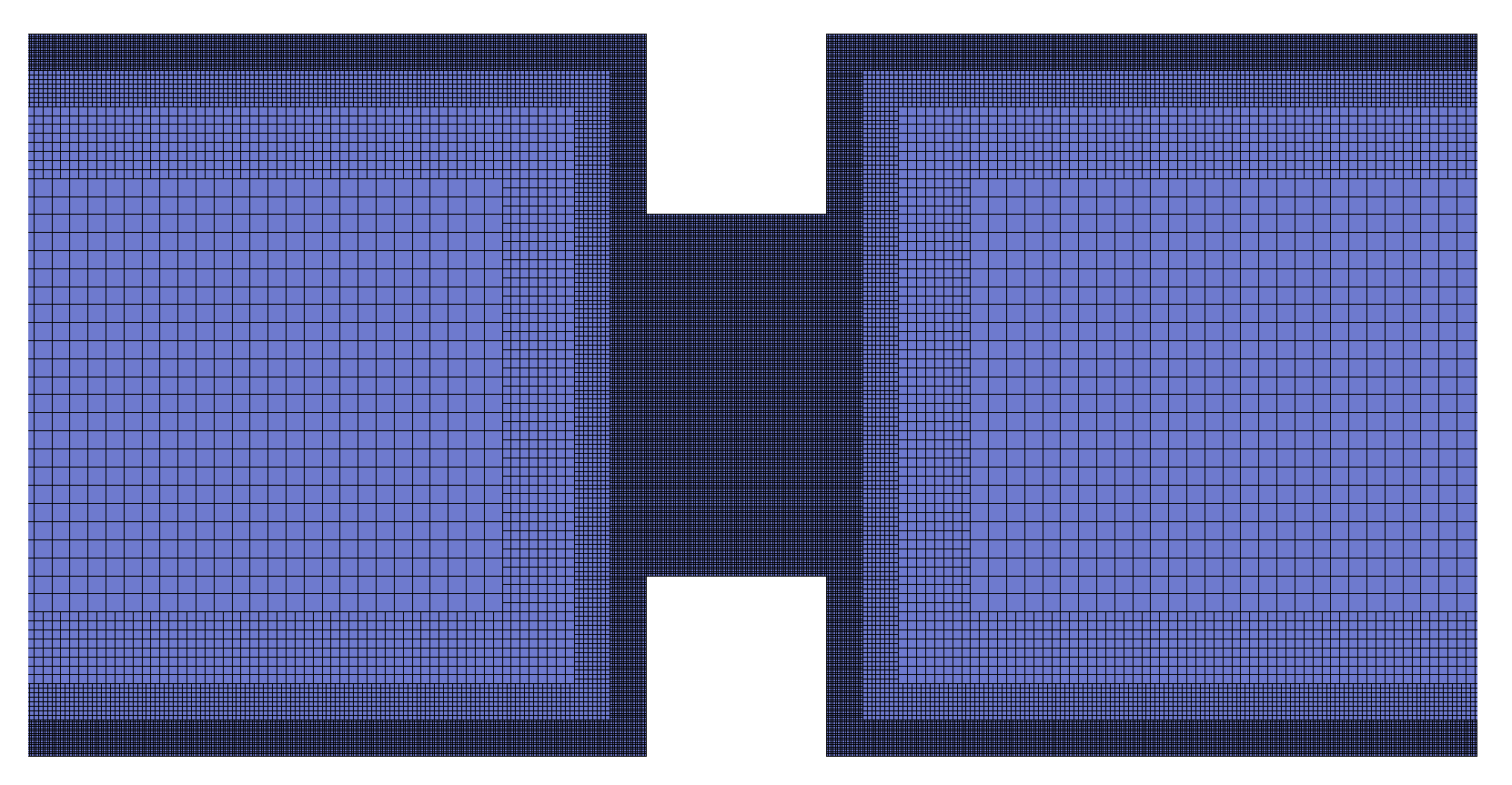
3. Computational Procedures
3.1. Boundary Conditions on the Walls
3.2. Inflow and Outflow
4. Results
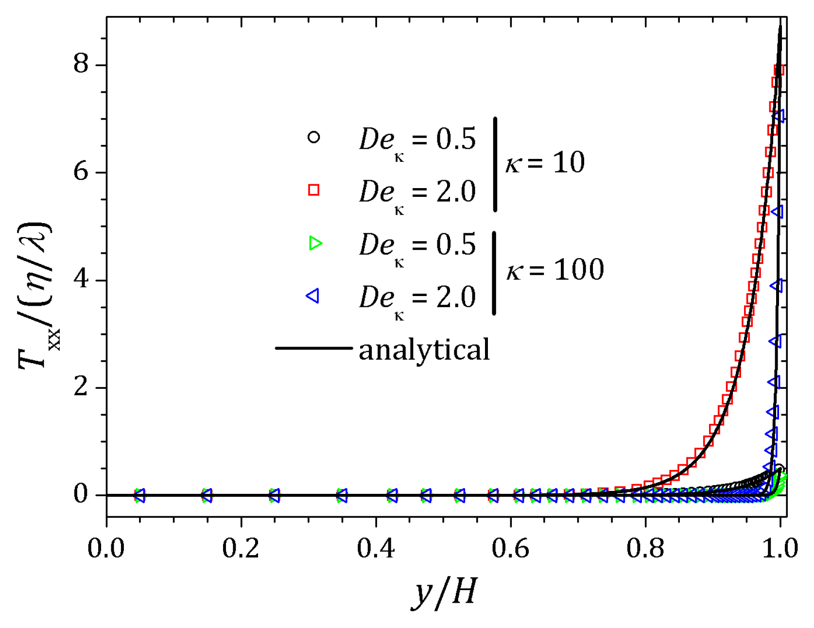
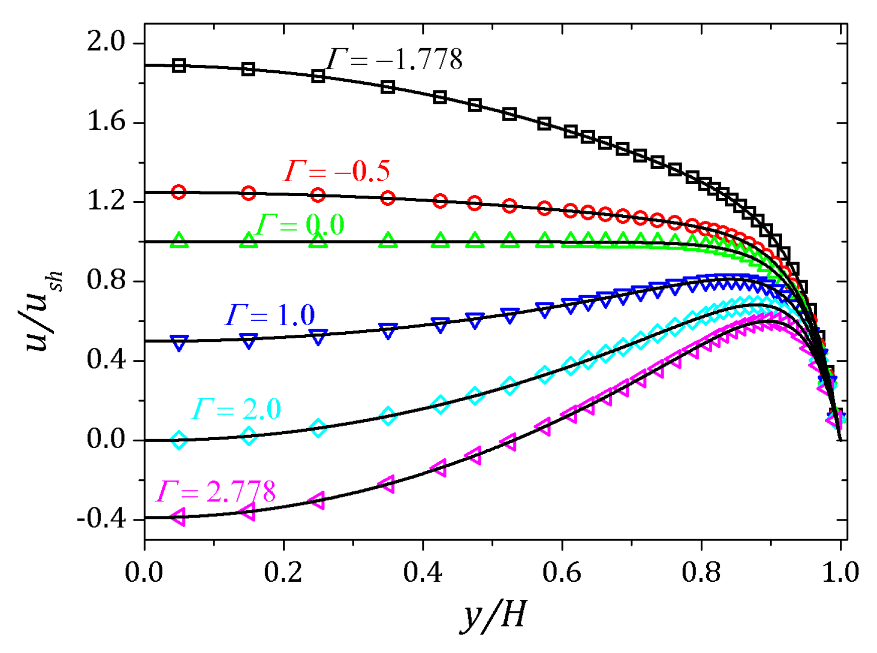
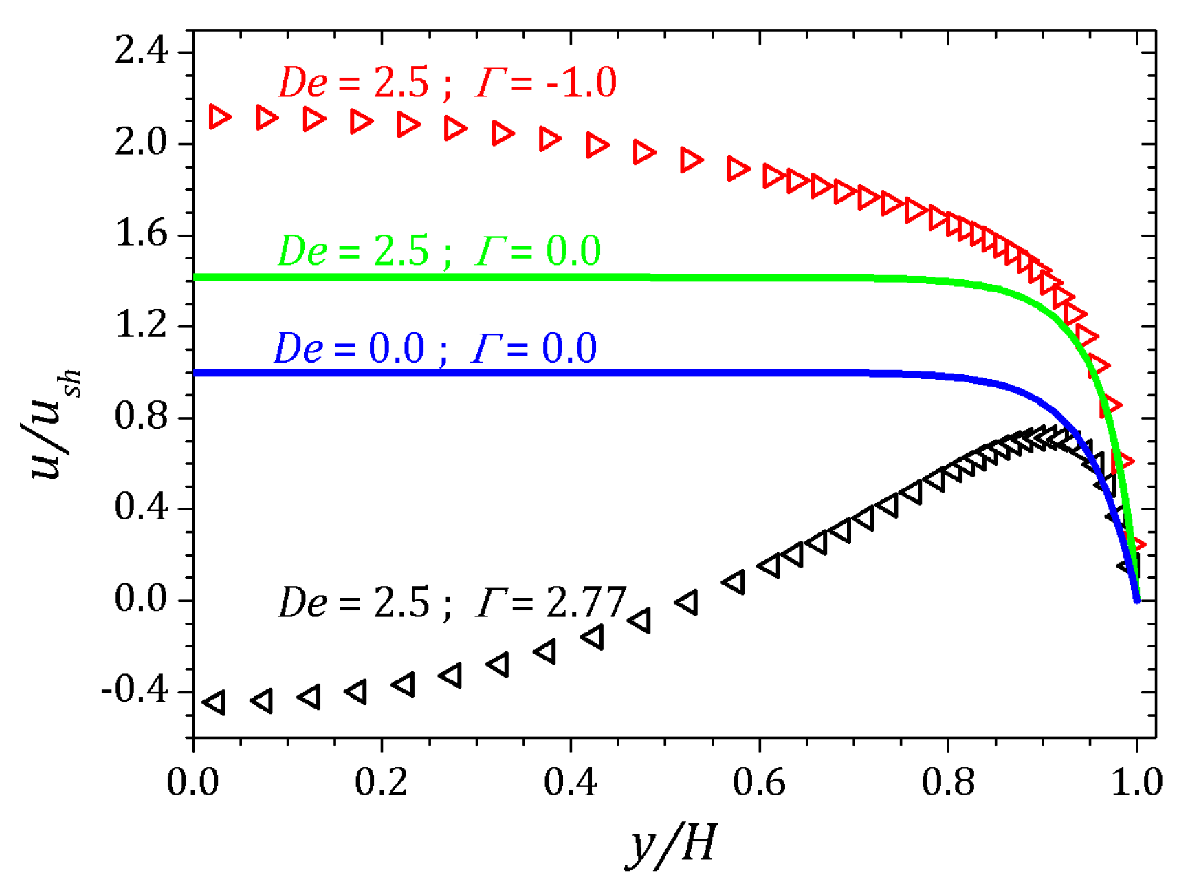
4.1. PTT Model
4.2. sPTT Model
4.3. Fluid Flow in a Nozzle
5. Conclusions
Author Contributions
Funding
Conflicts of Interest
References
- Doherty, E.A.; Meagher, R.J.; Albarghouthi, M.N.; Barron, A.E. Microchannel wall coatings for protein separations by capillary and chip electrophoresis. Electrophoresis 2003, 24, 34–54. [Google Scholar] [CrossRef] [PubMed]
- Chabinyc, M.L.; Chiu, D.T.; McDonald, J.C.; Stroock, A.D.; Christian, J.F.; Karger, A.M.; Whitesides, G.M. An integrated fluorescence detection system in poly (dimethylsiloxane) for microfluidic applications. Anal. Chem. 2001, 73, 4491–4498. [Google Scholar] [CrossRef] [PubMed]
- Bruus, H. Theoretical Microfluidics. Oxford Master Series in Condensed Matter Physics; Oxford University Press: Oxford, UK, 2008. [Google Scholar]
- Reuss, F.F. Sur un nouvel effet de l’électricité galvanique. Mem. Soc. Imp. Nat. Moscou 1809, 2, 327–337. [Google Scholar]
- Helmholtz, H.V. Studien über electrische Grenzschichten. Ann. Phys. 1879, 243, 337–382. [Google Scholar] [CrossRef]
- Gouy, M. Sur la constitution de la charge électrique à la surface d’un électrolyte. J. Phys. Theor. Appl. 1910, 9, 457–468. [Google Scholar] [CrossRef]
- Chapman, D.L.; LI. A contribution to the theory of electrocapillarity. Lond. Edinb. Dublin Philos. Mag. J. Sci. 1913, 25, 475–481. [Google Scholar] [CrossRef]
- Smoluchowski, M.V. Versuch einer mathematischen Theorie der Koagulationskinetik kolloider Lösungen. Z. Phys. Chem. 1918, 92, 129–168. [Google Scholar] [CrossRef]
- Debye, P.; Hückel, E. De la theorie des electrolytes. I. abaissement du point de congelation et phenomenes associes. Phys. Z. 1923, 24, 185–206. [Google Scholar]
- Burgreen, D.; Nakache, F. Electrokinetic flow in ultrafine capillary slits1. J. Phys. Chem. 1964, 68, 1084–1091. [Google Scholar] [CrossRef]
- Rice, C.; Whitehead, R. Electrokinetic flow in a narrow cylindrical capillary. J. Phys. Chem. 1965, 69, 4017–4024. [Google Scholar] [CrossRef]
- Yang, C.; Li, D. Analysis of electrokinetic effects on the liquid flow in rectangular microchannels. Colloids Surf. Physicochem. Eng. Asp. 1998, 143, 339–353. [Google Scholar] [CrossRef]
- Patankar, N.A.; Hu, H.H. Numerical simulation of electroosmotic flow. Anal. Chem. 1998, 70, 1870–1881. [Google Scholar] [CrossRef] [PubMed]
- Bianchi, F.; Ferrigno, R.; Girault, H. Finite element simulation of an electroosmotic-driven flow division at a T-junction of microscale dimensions. Anal. Chem. 2000, 72, 1987–1993. [Google Scholar] [CrossRef] [PubMed]
- Dutta, P.; Beskok, A. Analytical solution of combined electroosmotic/pressure driven flows in two-dimensional straight channels: finite Debye layer effects. Anal. Chem. 2001, 73, 1979–1986. [Google Scholar] [CrossRef]
- Lin, J.; Fu, L.M.; Yang, R.J. Numerical simulation of electrokinetic focusing in microfluidic chips. J. Micromech. Microeng. 2002, 12, 955. [Google Scholar] [CrossRef]
- Park, H.; Lee, W. Helmholtz–Smoluchowski velocity for viscoelastic electroosmotic flows. J. Colloid Interface Sci. 2008, 317, 631–636. [Google Scholar] [CrossRef]
- Zhao, C.; Zholkovskij, E.; Masliyah, J.H.; Yang, C. Analysis of electroosmotic flow of power-law fluids in a slit microchannel. J. Colloid Interface Sci. 2008, 326, 503–510. [Google Scholar] [CrossRef]
- Tang, G.; Li, X.; He, Y.; Tao, W. Electroosmotic flow of non-Newtonian fluid in microchannels. J. Non-Newton. Fluid Mech. 2009, 157, 133–137. [Google Scholar] [CrossRef]
- Afonso, A.; Alves, M.; Pinho, F. Analytical solution of mixed electro-osmotic/pressure driven flows of viscoelastic fluids in microchannels. J. Non-Newton. Fluid Mech. 2009, 159, 50–63. [Google Scholar] [CrossRef]
- Peng, R.; Li, D. Effects of ionic concentration gradient on electroosmotic flow mixing in a microchannel. J. Colloid Interface Sci. 2015, 440, 126–132. [Google Scholar] [CrossRef]
- Song, L.; Yu, L.; Zhou, Y.; Antao, A.R.; Prabhakaran, R.A.; Xuan, X. Electrokinetic instability in microchannel ferrofluid/water co-flows. Sci. Rep. 2017, 7, 46510. [Google Scholar] [CrossRef] [PubMed]
- Niu, R.; Kreissl, P.; Brown, A.T.; Rempfer, G.; Botin, D.; Holm, C.; Palberg, T.; De Graaf, J. Microfluidic pumping by micromolar salt concentrations. Soft Matter 2017, 13, 1505–1518. [Google Scholar] [CrossRef] [PubMed]
- Niu, R.; Palberg, T.; Speck, T. Self-assembly of colloidal molecules due to self-generated flow. Phys. Rev. Lett. 2017, 119, 028001. [Google Scholar] [CrossRef] [PubMed]
- Botin, D.; Wenzl, J.; Niu, R.; Palberg, T. Colloidal electro-phoresis in the presence of symmetric and asymmetric electro-osmotic flow. Soft Matter 2018, 14, 8191–8204. [Google Scholar] [CrossRef]
- Niu, R.; Palberg, T. Seedless assembly of colloidal crystals by inverted micro-fluidic pumping. Soft Matter 2018, 14, 3435–3442. [Google Scholar] [CrossRef]
- Arcos, J.; Méndez, F.; Bautista, E.; Bautista, O. Dispersion coefficient in an electro-osmotic flow of a viscoelastic fluid through a microchannel with a slowly varying wall zeta potential. J. Fluid Mech. 2018, 839, 348–386. [Google Scholar] [CrossRef]
- Pimenta, F.; Alves, M.A. Electro-elastic instabilities in cross-shaped microchannels. J. Non-Newton. Fluid Mech. 2018, 259, 61–77. [Google Scholar] [CrossRef]
- Fattal, R.; Kupferman, R. Constitutive laws for the matrix-logarithm of the conformation tensor. J. Non-Newton. Fluid Mech. 2004, 123, 281–285. [Google Scholar] [CrossRef]
- Fattal, R.; Kupferman, R. Time-dependent simulation of viscoelastic flows at high Weissenberg number using the log-conformation representation. J. Non-Newton. Fluid Mech. 2005, 126, 23–37. [Google Scholar] [CrossRef]
- Afonso, A.; Pinho, F.; Alves, M. The kernel-conformation constitutive laws. J. Non-Newton. Fluid Mech. 2012, 167, 30–37. [Google Scholar] [CrossRef]
- Sousa, F.S.; Lages, C.F.A.; Ansoni, J.L.; Castelo, A.; Simao, A. A finite difference method with meshless interpolation for fluid flow simulations in hierarchical grids. J. Comput. Phys. 2019, 396, 848–866. [Google Scholar] [CrossRef]
- Phan-Thien, N. A nonlinear network viscoelastic model. J. Rheol. 1978, 22, 259–283. [Google Scholar] [CrossRef]
- Thien, N.P.; Tanner, R.I. A new constitutive equation derived from network theory. J. Non-Newton. Fluid Mech. 1977, 2, 353–365. [Google Scholar] [CrossRef]
- Grahame, D.C. The electrical double layer and the theory of electrocapillarity. Chem. Rev. 1947, 41, 441–501. [Google Scholar] [CrossRef]
- Castelo, A.; Afonso, A.; Souza, W. A finite difference method in hierarquical grids for viscoelastic fluid flow simulations. J. Non-Newton. Fluid Mech. 2019. submitted. [Google Scholar]
- Finkel, R.A.; Bentley, J.L. Quad trees a data structure for retrieval on composite keys. Acta Inform. 1974, 4, 1–9. [Google Scholar] [CrossRef]
- Balay, S.; Abhyankar, S.; Adams, M.F.; Brown, J.; Brune, P.; Buschelman, K.; Dalcin, L.; Eijkhout, V.; Gropp, W.D.; Kaushik, D.; et al. PETSc Web Page. 2017. Available online: http://www.mcs.anl.gov/petsc (accessed on 20 November 2019).
- Afonso, A.; Pinho, F.; Alves, M. Electro-osmosis of viscoelastic fluids and prediction of electro-elastic flow instabilities in a cross slot using a finite-volume method. J. Non-Newton. Fluid Mech. 2012, 179, 55–68. [Google Scholar] [CrossRef]
- Ae, C.; Yang, R.J. Vortex generation in electroosmotic flow passing through sharp corners. In Microfluidics and Nanofluidics; Springer: Berlin/Heidelberg, Germany, 2008; Volume 5. [Google Scholar]
- Probstein, R.F. Physicochemical Hydrodynamics: An Introduction; John Wiley & Sons: Hoboken, NJ, USA, 2005. [Google Scholar]


© 2019 by the authors. Licensee MDPI, Basel, Switzerland. This article is an open access article distributed under the terms and conditions of the Creative Commons Attribution (CC BY) license (http://creativecommons.org/licenses/by/4.0/).
Share and Cite
Bezerra, W.D.S.; Castelo, A.; Afonso, A.M. Numerical Study of Electro-Osmotic Fluid Flow and Vortex Formation. Micromachines 2019, 10, 796. https://doi.org/10.3390/mi10120796
Bezerra WDS, Castelo A, Afonso AM. Numerical Study of Electro-Osmotic Fluid Flow and Vortex Formation. Micromachines. 2019; 10(12):796. https://doi.org/10.3390/mi10120796
Chicago/Turabian StyleBezerra, Wesley De Souza, Antonio Castelo, and Alexandre M. Afonso. 2019. "Numerical Study of Electro-Osmotic Fluid Flow and Vortex Formation" Micromachines 10, no. 12: 796. https://doi.org/10.3390/mi10120796
APA StyleBezerra, W. D. S., Castelo, A., & Afonso, A. M. (2019). Numerical Study of Electro-Osmotic Fluid Flow and Vortex Formation. Micromachines, 10(12), 796. https://doi.org/10.3390/mi10120796