Saliency Analysis via Hyperparameter Sparse Representation and Energy Distribution Optimization for Remote Sensing Images

Abstract

In an effort to detect the region-of-interest (ROI) of remote sensing images with complex data distributions, sparse representation based on dictionary learning has been utilized, and has proved able to process high dimensional data adaptively and efficiently. In this paper, a visual attention model uniting hyperparameter sparse representation with energy distribution optimization is proposed for analyzing saliency and detecting ROIs in remote sensing images. A dictionary learning algorithm based on biological plausibility is adopted to generate the sparse feature space. This method only focuses on finite features, instead of various considerations of feature complexity and massive parameter tuning in other dictionary learning algorithms. In another portion of the model, aimed at obtaining the saliency map, the contribution of each feature is evaluated in a sparse feature space and the coding length of each feature is accumulated. Finally, we calculate the segmentation threshold using the saliency map and obtain the binary mask to separate the ROI from the original images. Experimental results show that the proposed model achieves better performance in saliency analysis and ROI detection for remote sensing images.

1. Introduction

With the rapid progress of remote sensing technology, it is becoming easier to acquire high spatial resolution remote sensing images from various satellites and sensors. However, the analysis and processing of high spatial resolution images in more effective and efficient ways still remains a great challenge, particularly in images with complicated spatial information, clear details, and well-defined geographical objects [1,2,3,4].

The detection of the region of interest (ROI) has become a popular research topic, with valuable applications in many fields, such as object segmentation [5,6], image compression [7,8], video summarization [9], and photo collage [10,11]. Introducing ROI detection into remote sensing image processing has raised great concern among some scholars.

The human visual system serves as a filter for selecting a certain subset of visual information, based on visual saliency, while ignoring irrelevant information for further processing [12,13]. The region that draws human attention in an image is called ROI. There has been a lot of work done on saliency analysis and ROI extraction based on visual saliency, which is generally constructed based on low-level visual features, pure computation or a combination of these.

Itti et al. [14] developed a biologically-based model ITTI, which was named after the presenter, using “Difference of Gaussians” across multiple scales to implement “center-surround” contrast in color, intensity, and orientation features. Li et al. [15] presented a model based on Itti’s method and additionally extracted GIST features trained by a support vector machine (SVM). Klein et al. [16] extracted ROIs with the knowledge of information theory. Although the models calculated visual saliency based on biological plausibility, the computing of center-surround involved the tuning of many parameters that determined the final performance.

In addition, pure computation based algorithms for ROI extraction have also been developed. Saliency analysis based on frequency domain has been shown in [17,18,19]. Imamoglu et al. [20] utilized the lower-level features produced by wavelet transform (WT). The above methods based on pure computing improve the efficiency of saliency processing. However, problems related to the complexity of modeling catering to different feature distributions and the lack of sufficient plausibility of biological visual saliency mechanisms are still unsolved.

With regard to mixed models, the Graph-based visual saliency (GBVS) model proposed by Harel et al. [21] applied the principles of Markov Chain theory to normalize activation maps on each extracted feature under the ITTI model. In 2012, Borji and Itti [22] utilized the sparse representation of the image and used local and global contrast in combination to detect saliency. Goferman et al. [23] combined local underlying clues and visual organization rules with methods of local contrast to highlight significant objects, and proposed a different model based on context-aware (CA) salient information. The CA model can detect the salient object in certain scenes, but the inevitably high false detection rate affects the accuracy. Another drawback of the model is that the time complexity is much higher than for other spatial-based saliency models. Wang et al. [24] proposed a visual saliency model based on selective contrast. Additionally, methods utilizing learning have also attracted attention in recent years, such as the model for saliency detection by multiple-instance learning [25].

In terms of the application of saliency analysis in remote sensing images, some have employed support vector machines (SVM) to extract bridges and airport runways from remote sensing images [26,27]. Some have constructed parameterized models to extract roads and airports from remote sensing images with prior information of targets [28,29,30]. Zhang et al. [31] proposed a frequency domain analysis (FDA) model based on the principle of Quaternion Fourier Transform to attain better experimental results compared with those that only used the information of amplitude spectrum or phase spectrum in the frequency domain. Zhang et al. also adopted multi-scale feature fusion (MFF) based on integer wavelet transform (IWT) to extract residential areas along the feature channels of intensity and orientation [32]. For some remote sensing images corrupted by noise, the saliency analysis of co-occurrence histogram (SACH) model uses a co-occurrence histogram to improve robustness against Gaussian and Salt and Pepper noises [33]. In addition, global clustering methods for image pre-classification or ROI detection are also introduced in remote sensing images [34,35,36]. For example, Lu et al. [36] first produced an initial clustering map, and then utilized a multiscale cluster histogram to analyze the spatial information around each pixel.

It is noticeable that the data sets of remote sensing images have a high volume of dimensional information, which is usually too large to handle effectively. Aiming at this problem, sparse codes have been introduced into image processing. Sparse codes learned from image patches are similar to the receptive fields of simple-cells in the primary visual cortex (V1) [37], which shows that the mechanism of human visual saliency is consistent with sparse representation. Sparse representation has also been shown to be a quite effective technique for wiping out non-essential or irrelevant information in order to reduce the dimensions. Furthermore, it has greater flexibility for data structure capture, and better stability against perturbations of the signal, which suggests that we can obtain the sparse coefficients produced by those basic functions with good robustness against noise or corruption.

Researchers have proposed a number of methods for dictionary learning. Independent Component Analysis (ICA) is a good method for learning a dictionary in order to obtain compact basic functions. Thus, ICA is mainly utilized for the learning of basic functions based on a large number of randomly selected image patches. In addition, there are also some other methods, such as DCT [38], DWT [39], K-SVD [40], and FOCUSS [41], which also perform well at forming sparse representation of datasets.

However, these methods are difficult to use when faced with different data modalities requiring specific extensive hyper-parameter tuning on each modality when learning a dictionary in remote sensing images. For DCT and DWT, there are three parameters that need to be considered: the number of extracted features; the sparsity penalty, which is used to balance sparsity and distortion during the learning process; and the size of mini-batch, which helps improve processing efficiency. For K-SVD, sparsity and dictionary size of the target should also be considered. For FOCUSS, the calculation of the final results needs a posteriori information. Therefore, the efficiency of these dictionary learning algorithms may run into a bottleneck when applied to remote sensing images.

Considering the problems mentioned above, we propose a model based on the integration of hyperparameter sparse representation and energy distribution optimization for saliency analysis. In this study, we focus on the ROI in optical remote sensing images. As a whole, the combination has full biological plausibility in terms of the human visual mechanism. In terms of sparse representation of remote sensing images, we adopt a novel feature learning algorithm—hyperparameter sparse representation—to train a dictionary. This algorithm is simple, clear and can be quickly implemented with high effectiveness, as well as being almost parameter-free, as the feature number is the only item to be decided. As for the measure of saliency, we use an energy distribution optimization algorithm to define saliency as entropy gain. Similarly, computation of this algorithm does not involve any parameter tuning, and is computationally efficient.

In the experimental process, we first transform the image from the RGB color space to the HSI color space as a preprocessing step. Subsequently, the input remote sensing images are divided into overlapping patches, and the patches are further decomposed over the learned dictionary. Then, an algorithm is utilized to maximize the entropy of visual saliency features for energy redistribution, so as to generate a final saliency map. Finally, Otsu’s threshold segmentation method is implemented in the acquisition of binary masks from saliency maps, and the masks are then used for ROI extraction from the original remote sensing images. Experimental results show that the proposed model achieves better performance than other traditional models for saliency analysis of and ROI detection in remote sensing images.

There are three major contributions in our paper: (1) we introduce hyperparameter sparse representation into dictionary learning for remote sensing images. The algorithm converges faster and has fewer parameters; (2) while training the dictionary, we define every single pixel as a feature. Thus, the sparse representation of an image is equal to the optimal features used for further saliency analysis; and (3) hyperparameter sparse representation and energy distribution optimization of features are integrated to compute the saliency map. This method is biologically rational, and consistent with cortical visual information processing.

The work in this paper is organized as followed: the proposed model is thoroughly illustrated in Section 2, Section 3 focuses on the experimental results and discussion, Section 4 and Section 5 provide the applications and conclusion, respectively.

2. Methodology

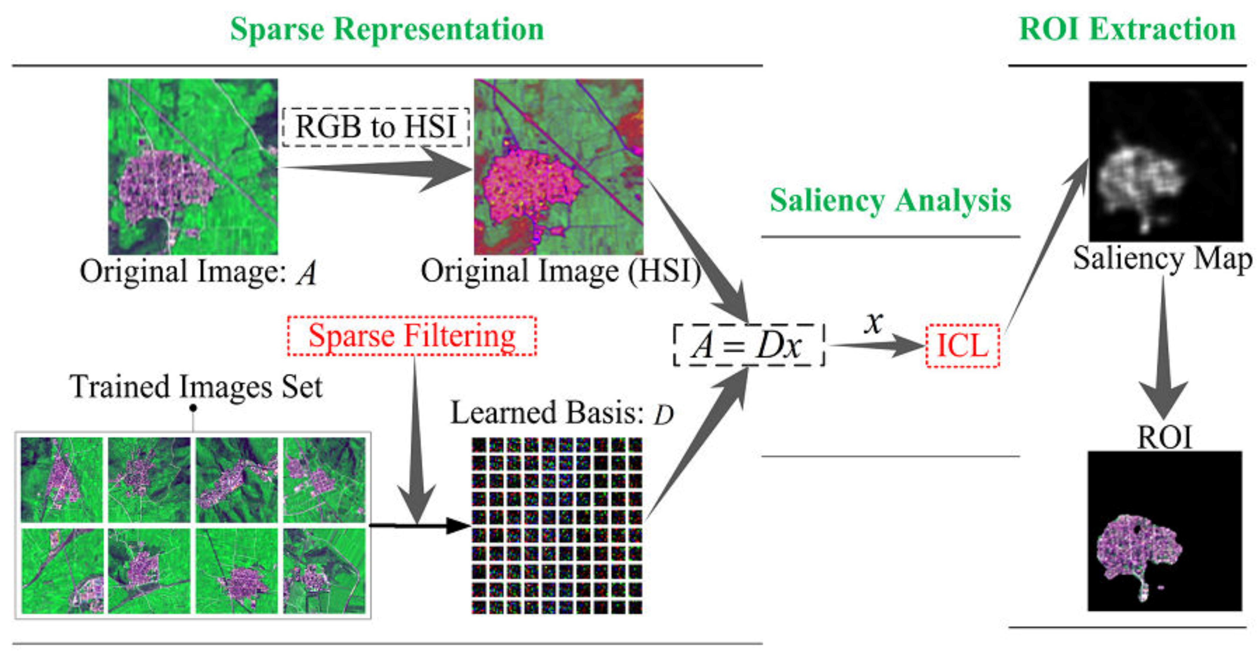
In the proposed model, the whole process of ROIs detection for remote sensing images can be divided into three parts: (1) obtain sparse representation of the image feature; (2) compute saliency contribution of all sparse features; (3) extract the ROIs from saliency maps. Figure 1 illustrates the framework of the proposed model. As we can see, in the first part, an unsupervised feature learning algorithm—Hyperparameter Sparse Representation—is utilized to create a dictionary for sparse representation of remote sensing images. We define every single pixel as a feature. Thus, the sparse representation of an image is equal to the optimal features that are used for further saliency analysis. The second part measures the entropy gain of each feature. On the basis of the general principle of predictive coding [42], the rarity of features can be seen as their average energy, which is redistributed to features in terms of their code length: frequently activated features receive less energy. The final saliency map is generated by summing up the activity of all features. Finally, we segment ROI from the original remote sensing image with the mask of saliency map based on the threshold segmentation algorithm [43].

Due to the characters of the simple computation, time efficiency and consistency in terms of the human color perception system of an HSI-based model [44], we preprocess images from RGB to HSI color space. Then the represented image is divided into overlapping patches and each patch is vectored as a column where all the pixel features were columned to form a feature matrix. Section 2.2, Section 2.3, Section 2.4 separately introduce the details of the three parts of our proposed model.

2.1. The Inadequacy of Traditional Algorithms

As we mentioned in Section 1, traditional visual saliency analysis methods have played an increasingly important role in the field of remote sensing image processing. Remote sensing images generally have high resolution and complex structure, which means that it is difficult to process directly. Visual attention models are first proposed for natural scene images. This kind of image is mostly obtained by different types of cameras, which means that we can highlight the significant targets by adjusting the aperture and the shutter. Targets will contain more information than background by selecting artificially. However, in remote sensing images, all objects have the same clarity. In other words, there is no difference in terms of clarity between the residential areas and the mountains, the roads and the ponds. Because of the clear and complex background, the problem of background interference is serious, which makes the saliency analysis hard.

The traditional methods need to combine the difference of the data distribution characteristics to select the effective calculation method for analysis, which will undoubtedly increase the diversity and complexity of the analysis. Moreover, the primary visual cortex shows that the receptive field of the single cell is similar to the sparse coding of the natural image block [45]. The human visual system also exhibits the characteristics of multilayer sparse representation of the image data. It shows that the sparse representation is consistent with the principle of human visual saliency mechanism, and can well explain the visual significance, which is biologically rational.

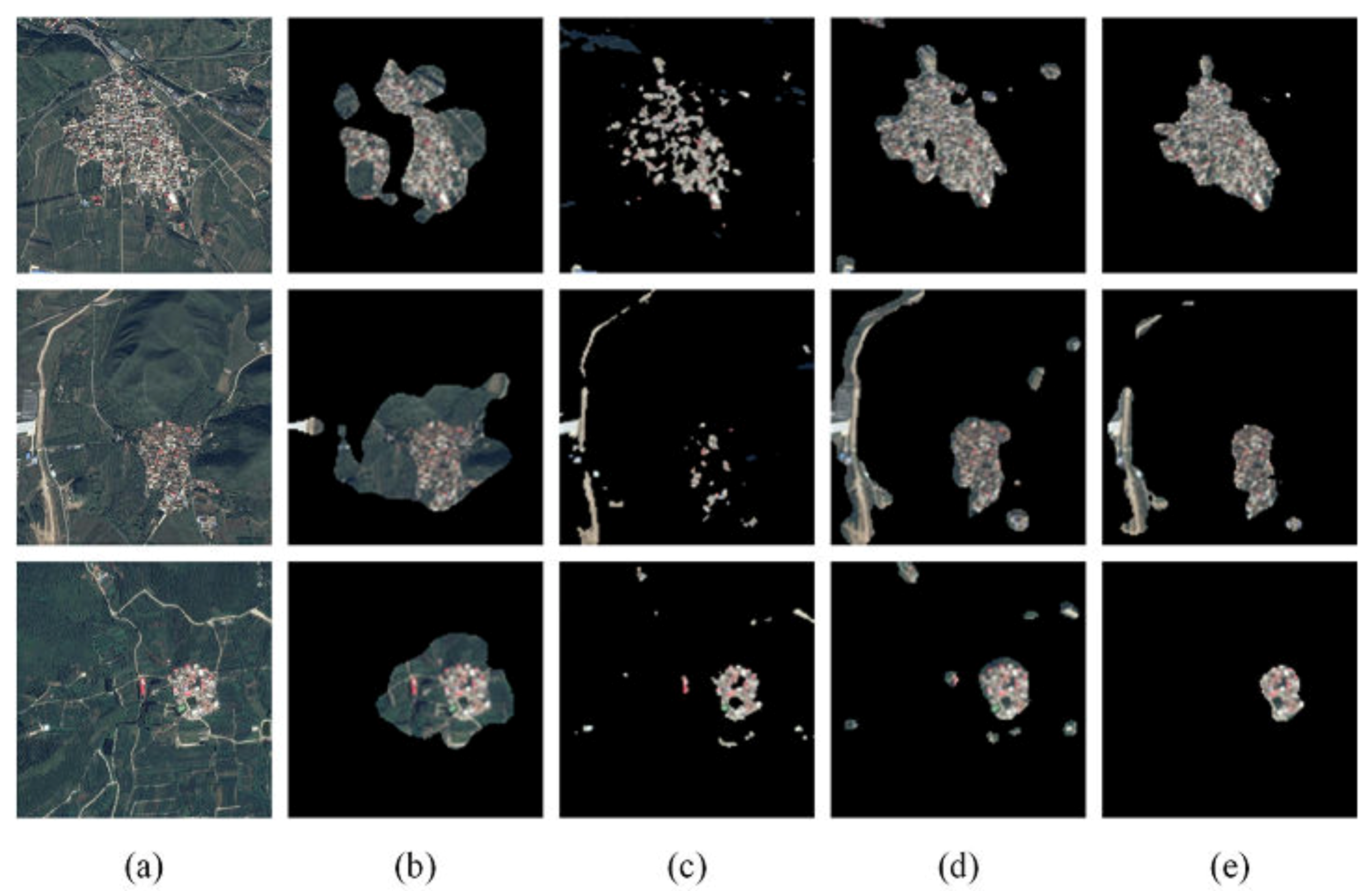
As shown in Figure 2, the ITTI model always mistakenly detects the background and sometimes misses the target region. The results of the frequency domain based model, Frequency-tuned (FT) model, contain a lot of debris and holes. The algorithms, which are designed specifically for ROI detection of remote sensing images, FDA and our model, obtain acceptable results. However, our results are clearly more accurate. In general, the ITTI and FT model are likely to get more inaccurate results, the FDA model makes some relative progress, and our model works best.

2.2. Hyperparameter Sparse Representation

The method of dictionary learning can be considered as the generation of a particular feature distribution. For example, sparse representations are designed to use several nonzero coefficients to represent each sample, which highlight the main features of the sample. To achieve this goal, the ideal characteristics of the feature distribution should be optimized.

The desirable properties of feature distribution should meet with and include the three criteria [46]: population sparsity, lifetime sparsity and high dispersal. Population sparsity means that for each column in the feature matrix, there should be finite active (non-zero) elements. Moreover, it provides an effective coding method which is a theoretical basis for early visual cortex studies. Lifetime sparsity refers to that each row of feature matrix having only a small number of non-zero elements. This is because the features which are needed for further calculation ought to be characteristic of discrimination. High dispersal indicates that all features should have similar contributions, and the activity value of each row is supposed to be the same for every feature. Under certain circumstances, high dispersal is not completely necessary for good feature representation, on account of the same features which may be active and can prevent feature degeneration [46].

According to the characteristics that the sparse features should have, we apply a simple algorithm—hyperparameter sparse representation—which can optimize the three properties of features. Specifically, we illustrate these properties with a feature matrix of each sample. Figure 3 shows the structure of this algorithm.

Each pixel column is viewed as a feature in our model. A feature matrix will be obtained after remote sensing image preprocessing. Each row of the matrix represents a feature and each column is a patch divided from the image. $f_j^{\mathit{(}i\mathit{)}}$ represents the jth feature value (rows) for the ith patch (columns). This sparse representation method aims to optimize and normalize the feature matrix by rows (feature values), then by columns (vectored image patch) and finally sums up the absolute value of all entries.

Firstly, by dividing each feature by its $l_2$-norm across all patches, each feature is normalized to be equally active:

$$\stackrel{\cap }{f_j}=f_j\mathit{/}{\Vert f_j\Vert }_2$$

(1)

Then, analogously, by computing $\stackrel{\wedge }{f^{\mathit{(}i\mathit{)}}}=\stackrel{\cap }{f^{\mathit{(}i\mathit{)}}}\mathit{/}\stackrel{\cap }{\Vert f^{\mathit{(}i\mathit{)}}{\Vert }_2}$, all these features are normalized by each patch to put them on the $l_2$-norm ball. All normalized features are further optimized for sparsity by $l_1$ penalty. If there are $M$ patches, then the sparse filtering objective function can be written as follows:

$$\mathit{min}{{\displaystyle \sum _{i=1}^M}{\Vert \stackrel{\wedge }{f^{\mathit{(}i\mathit{)}}}\Vert }_1={\displaystyle \sum _{i=1}^M}\Vert \frac{\stackrel{\cap }{f^{\mathit{(}i\mathit{)}}}}{{\Vert \stackrel{\cap }{f^{\mathit{(}i\mathit{)}}}\Vert }_2}\Vert }_1$$

(2)

Now it is essential to analyze whether the objective function meets with the three properties of desire features. First, population sparsity of features on the ith patch is measured by the equation as follows:

$${\stackrel{\wedge }{\Vert f^{(i)}\Vert }}_1={\Vert \frac{\stackrel{\cap }{f^{(i)}}}{{\Vert \stackrel{\cap }{f^{(i)}}\Vert }_2}\Vert }_1$$

(3)

when the features are sparse, an objective function can reach a minimum for the constraint of $\stackrel{\wedge }{f^{(i)}}$ in the $l_2$-norm ball. Contrarily, a patch that has similar values for each feature would incur a high penalty. Normalization of all features would cause competition between features: if only one element of $f^{(i)}$ increases, all the other elements in $f^{(i)}$ will decrease in the normalization, and vice versa. Minimal optimization of the objective function aims to make the normalization features sparse and mostly close to zero. With the principle of the competition between features, some features in $f^{(i)}$ have to be of large values while most of the rest of them are very small. To sum up, the objective function has been optimized for population sparsity.

Meanwhile, to satisfy the quality of high dispersion, each feature should equally active. As mentioned above, each feature is divided by its $l_2$-norm across all patches and normalized to be equally active by Equation (1). This is equal to constraining each feature to have the same expected squared value, thus contributing high dispersion. In the work of Ngiam et al. [47], they found that we can obtain over-complete sparse representation when realizing population sparsity and high dispersion in feature optimization, which also means that it is sufficient to learn good features as long as the condition of population sparsity and high dispersion are satisfied.

Therefore, obviously, the sparse filtering satisfies the three properties of desirable feature distribution and at the same time is also proved to be a fast and easy algorithm to implement. The entire optimization can be seen as the process of dictionary learning. When the objective function is optimized to reach a minimum under constraints, a dictionary $D$ for sparse representation of the original image would appear to be the natural next-step before going on to process the image.

Notably, the entire optimization process of the feature matrix is automatically operated with the only tunable parameter: the number of the features. We can change the number of features by resizing the row number of the feature matrix to satisfy different requirements in image and signal processing. We can also learn that the dictionary learning process of the proposed model is approximately similar to the multi-layer sparsity by which the human vision system reacts to an image with the salient region from its surroundings.

2.3. Energy Distribution Optimizing

In this part, we describe the saliency of images with the optimized energy distribution (Algorithm 1), where different feature responses should have different energy intensity based on the principle of predictive coding. Therefore, incremental coding length is introduced to measure the distribution of energy on different features [48], which implies that different features have different rarity. The energy of the jth feature is defined as the ensemble’s entropy gain during the activity of the jth feature. So the rarity of a dictionary feature is computed as its average energy. That is to say, rarely activated features will receive higher energy than activated ones. Then the final visually saliency is obtained by energy measurement, which shows that saliency computation by energy distribution conforms to the mechanism of human visual saliency in some degree.

Algorithm 1. Energy Distribution Optimizing

Input: A remote sensing image $A=\mathit{[}{a}_1,a_2,\cdots a_k,\cdots \mathit{]}$ and the liner filter $W=\mathit{[}{w}_1,w_2,\cdots w_k,\cdots \mathit{]}$.

Vectorize the image patch $a_k$

for each feature do

compute the activity ratio of the $j^{th}$ feature $p_j$.

maximize the entropy $H\mathit{(}\mathbf{p}\mathit{)}.$

when a new excitation add a variation $\epsilon$ to $p_i$

if $i=j$   $\stackrel{\wedge }{p_i}=\mathit{(}{p}_i+\epsilon \mathit{)}\mathit{/}\mathit{(}1+\epsilon \mathit{)}$

else      $\stackrel{\wedge }{p_i}=p_i\mathit{/}\mathit{(}1+\epsilon \mathit{)}$

end

calculate the change of entropy of the $j^{th}$ feature $COE\mathit{(}{p}_j\mathit{)}$.

get the salient features group $G=\mathit{\{}i|COE\mathit{(}{p}_i\mathit{)}>0\mathit{\}}$

compute the energy of the $j^{th}$ feature $d_j$

end

obtain the saliency map $m_k$ of image patch $a_k$

With the dictionary $D$ for sparse representation mentioned above, the spare feature matrix $X$ of image $A$ on $D$ can be acquired by $X=WA$, where $W=D^{-1}$. Then we can compute the activity ration $p_j$ as follows:

$$p_j=\frac{{\displaystyle {\sum }_k|w_j{a}_k|}}{{\displaystyle {\sum }_j{\displaystyle {\sum }_k|w_j{a}_k|}}}$$

(4)

To fully consider the reaction degree of each feature in the sparse code and achieve optimality, maximizing the entropy $H\mathit{(}\mathbf{p}\mathit{)}$ of the probability function $\mathbf{p}$ is a key principle to efficient coding. The probability function $\mathbf{p}$ varies at different points of time, depending upon whether there is a new perturbation on a feature, which means a variation $\epsilon$ will be added to $p_i$ and further change the whole probability distribution.

This variation will change the entropy of the feature activities. We define the change of entropy of the jth feature $COE\mathit{(}{p}_j\mathit{)}$ as the following equation:

$$COE\mathit{(}{p}_j\mathit{)}=\frac{\partial H\mathit{(}\mathbf{p}\mathit{)}}{\partial p_j}=-H\mathit{(}\mathbf{p}\mathit{)}-p_j-\mathit{log}{p}_j-p_j\mathit{log}{p}_j$$

(5)

The features with COE value above zero are viewed as salient and a salient feature set is obtained as G. Then the energy among features are redistributed according to their COE values. Denote the amount of energy that every sparse feature obtains $d_j$ is computed as follows:

$$d_j=\{\begin{array}{ccc}\frac{COE\mathit{(}{p}_j\mathit{)}}{{\displaystyle \sum _{j\in G}}COE\mathit{(}{p}_j\mathit{)}}& & j\in G\\ 0& & j\notin G\end{array}$$

(6)

Finally, the saliency map $M=\mathit{[}{m}_1,m_2,\cdots m_k,\cdots \mathit{]}$ of image A can be obtained as the equation below:

$$m_k={\displaystyle \sum _{j\in G}}{d}_j{w}_j{a}_k$$

(7)

The final saliency map can be obtained by restoring all the vectorization image patches to the whole original remote sensing image.

2.4. Threshold Segmentation

To further evaluate the performance of the proposed model, we segment the saliency maps from the original images and obtain masks of the ROIs with the threshold algorithm proposed by Otsu [43].

Assume that the total number of pixels in an image is $N$, gray values of the image range from 1 to L, and the number of pixels with gray value i in the entire image is $n_i$. The occurrence ratio of pixels is computed as follows:

$$p_i=n_i/N \mathit{(}i=1,2,\dots L\mathit{)}$$

$${\displaystyle \sum _{i=1}^L}{p}_i=1$$

(8)

Suppose that the gray threshold value is k, pixels of the whole image is thus divided into two classes: A and B. Values in class A range from 1 to k, and values in class B from k + 1 to L. Their respective ratio is:

$$\begin{array}{l}{\omega }_A={\displaystyle \sum _{i=1}^k}{p}_i=\omega \mathit{(}k\mathit{)}\\ {\omega }_B={\displaystyle \sum _{i=k+1}^k}{p}_i=1-\omega \mathit{(}k\mathit{)}\end{array}$$

(9)

Then, the average gray value of each cluster is:

$$\begin{array}{l}{\lambda }_A={\displaystyle \sum _{i=1}^k}i{p}_i/{\omega }_A=\frac{\lambda \mathit{(}k\mathit{)}}{\omega \mathit{(}k\mathit{)}}\\ {\lambda }_B={\displaystyle \sum _{i=1+k}^L}i{p}_i/{\omega }_B=\frac{{\lambda }_T-\lambda \mathit{(}k\mathit{)}}{1-\omega \mathit{(}k\mathit{)}}\end{array}$$

(10)

where $\lambda \mathit{(}k\mathit{)}={\displaystyle \sum _{i=1}^k}i{p}_i$ and ${\lambda }_T={\displaystyle \sum _{i=1}^L}i{p}_i$. ${\lambda }_T$ is the average gray value of the whole image. The variance between A and B are calculated as follows:

$${\sigma }^2\mathit{(}k\mathit{)}=\frac{{\mathit{[}{\lambda }_T\omega \mathit{(}k\mathit{)}-\lambda \mathit{(}k\mathit{)}\mathit{]}}^2}{\omega \mathit{(}k\mathit{)}\mathit{[}1-\omega \mathit{(}k\mathit{)}\mathit{]}}$$

(11)

Then, the optimal segmentation threshold can be obtained by:

$$k^{*}={\displaystyle \underset{1\le k\le L}{\mathit{arg}\mathit{max}}}{\sigma }^2\mathit{(}k\mathit{)}$$

(12)

The segmentation threshold value varies for different saliency maps. With the image binary segmentation, the masks of the ROIs are produced, and the masks are overlaid onto the original images to extract the final ROI in the next step.

3. Experimental Results and Discussion

To evaluate the performance of the proposed model, we used 300 remote sensing images of two different kinds as the experimental data. One is the remote sensing images from the SPOT 5 satellite with a spatial resolution of 2.5 m; the other is the remote sensing images from Google Earth with a higher spatial resolution of 1.0 m. The size of the experimental data are all 512 × 512 pixels. Among experiment images, we define the rural residential regions as ROIs, which should be detected primarily. As we have presented before, these regions typically include rich texture, irregular boundary, the area of brightness and color highlighting.

For the proposed model, the size of all these images used for learning a dictionary is down-sampled to 128 × 128 pixels, considering that we chose each pixel as a feature for saliency detection and ROI extraction. Therefore, the time consumed will be unbelievably excessive if we directly process images of original size. For remote sensing images of each kind, we randomly selected 60 images of to train the dictionary for sparse representation and all the 150 images were demonstrated for saliency analysis and ROIs extraction. The performance of the proposed model was compared qualitatively and quantitatively with other nine models including the Itti’s model (ITTI) [14], the frequency-tuned (FT) model [17], the spectral residual (SR) model [18], the Graph-based visual saliency (GBVS) model [21], the Wavelet-transform-based (WT) model [20], the context aware (CA) model [23], the multiscale feature fusion (MFF) model [32], the frequency domain analysis (FDA) model [31] and the saliency analysis of co-occurrence histogram (SACH) model [33]. These nine models are selected for the following reasons:

• high citation rate: The classic model ITTI and SR have been widely cited;
• variety: ITTI is biologically motivated; FT, SR, and WT model all are the purely computational based models and estimate saliency in the frequency domain; GBVS and CA both belong to biological models and partly to the computational model;
• affinity: MFF, FDA and SACH model all are specially designed for saliency analysis in remote sensing images.

Notably, we use resized original images of 128 × 128 pixels to test their respective performance on different models. Finally, we resized the saliency maps of all models uniformly to the size of 128 × 128 pixels for fair comparison. Here, in each kind of image, we choose eight out of all the 150 images to make up the display figures for our experimental results.

After the transformation from RGB to HSI color space, we divide all the input remote sensing images used for dictionary training into overlapped patches of the size of 8 × 8 pixels with 192-dimension and further form an up to 130,000 large set of vectorization image patches.

Here, what we should pay attention to is the selecting feature number which is the only tunable parameter in the process of dictionary learning. Generally, a greater numbers of features correlates to a better performance. For consistency with the input dimension of the vectorization image set to form a square matrix, we choose 192 features for dictionary learning and saliency analysis. In our experiments, we adopted the off-the-shelf L-BFGS [49] package to optimize the sparse filtering objective until convergence with a maximum iteration number of 100. The learned dictionary we have obtained is shown in Figure 4.

3.1. Qualitative Experiment

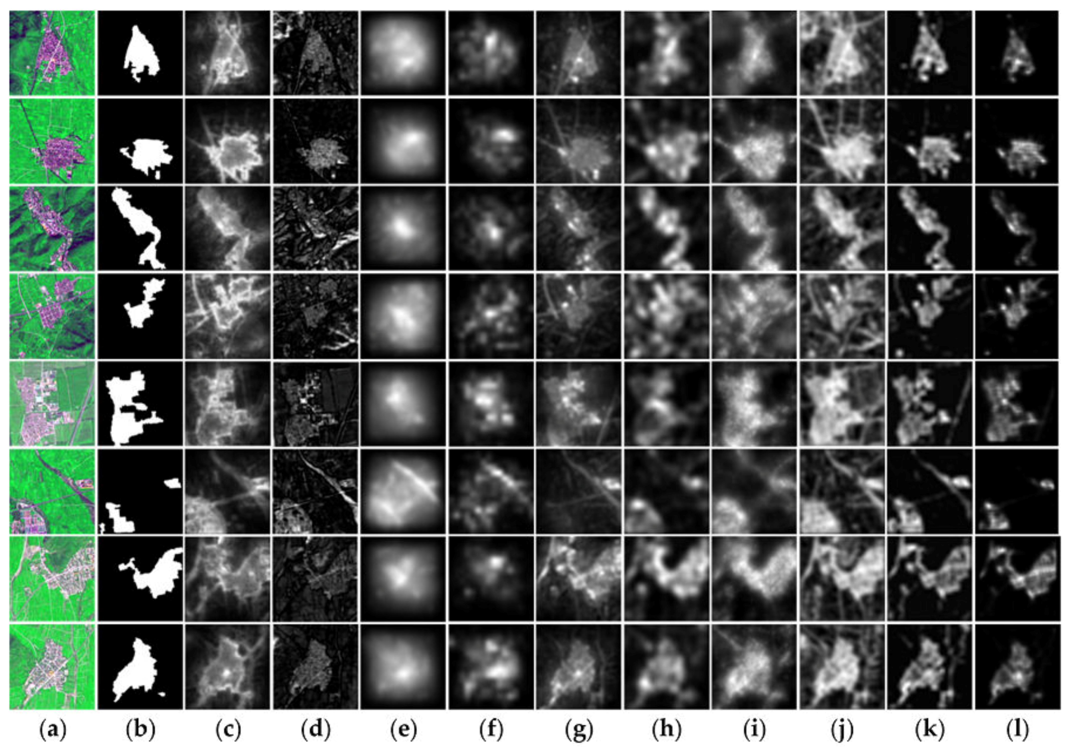
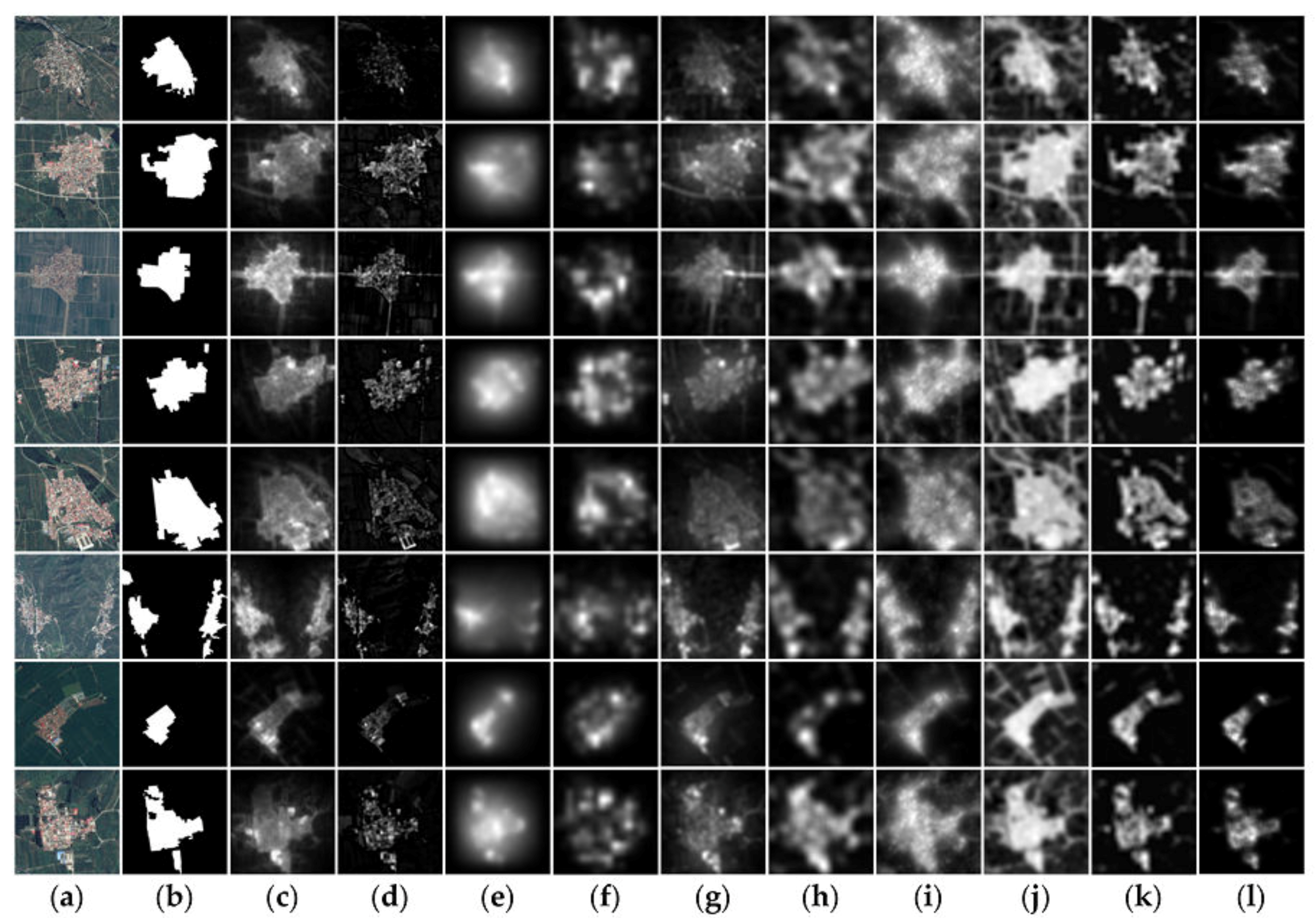
As shown in Figure 5 and Figure 6, the comparison among saliency maps generated by the proposed model and the other nine competing models on remote sensing images from SPOT 5 satellite and Google Earth, respectively. We can see that the saliency maps obtained by the proposed method focus on the residential areas and hardly have any background information. In contrast to the original images, the results of our model detected almost all salient objects. However, the other nine models detected some redundant information from the original images and cannot accurately locate the salient region. Although the CA model detects a clear boundary, it also includes the non-residential areas, thus enlarging the fall-out ratio and meanwhile is quite time-consuming.

For SPOT 5 images, the experimental results of FDA model seem close to ours but we can see that there are still some little non-salient regions such as roads contained in the last four saliency maps in Figure 5. The MFF and SACH model can also obtain saliency maps which are not bad, but they are not accurate enough. Other models such as the ITTI, GBVS, and SR generate the final saliency maps of low resolution with blurred boundaries, which do not contribute to further ROI extraction. The CA and WT model always get acceptable results, but the inevitable needless background information can always be highlighted, too. Conversely, FT model fails to highlight the entire salient area, which results in the so-called hole effect that is the incomplete description of the salient area’s interior. Meanwhile, for Google Earth images, although the performance of all the other models on saliency details such as border information is a little worse than that on SPOT images because of the higher spatial resolution, the proposed model still performs better intuitively.

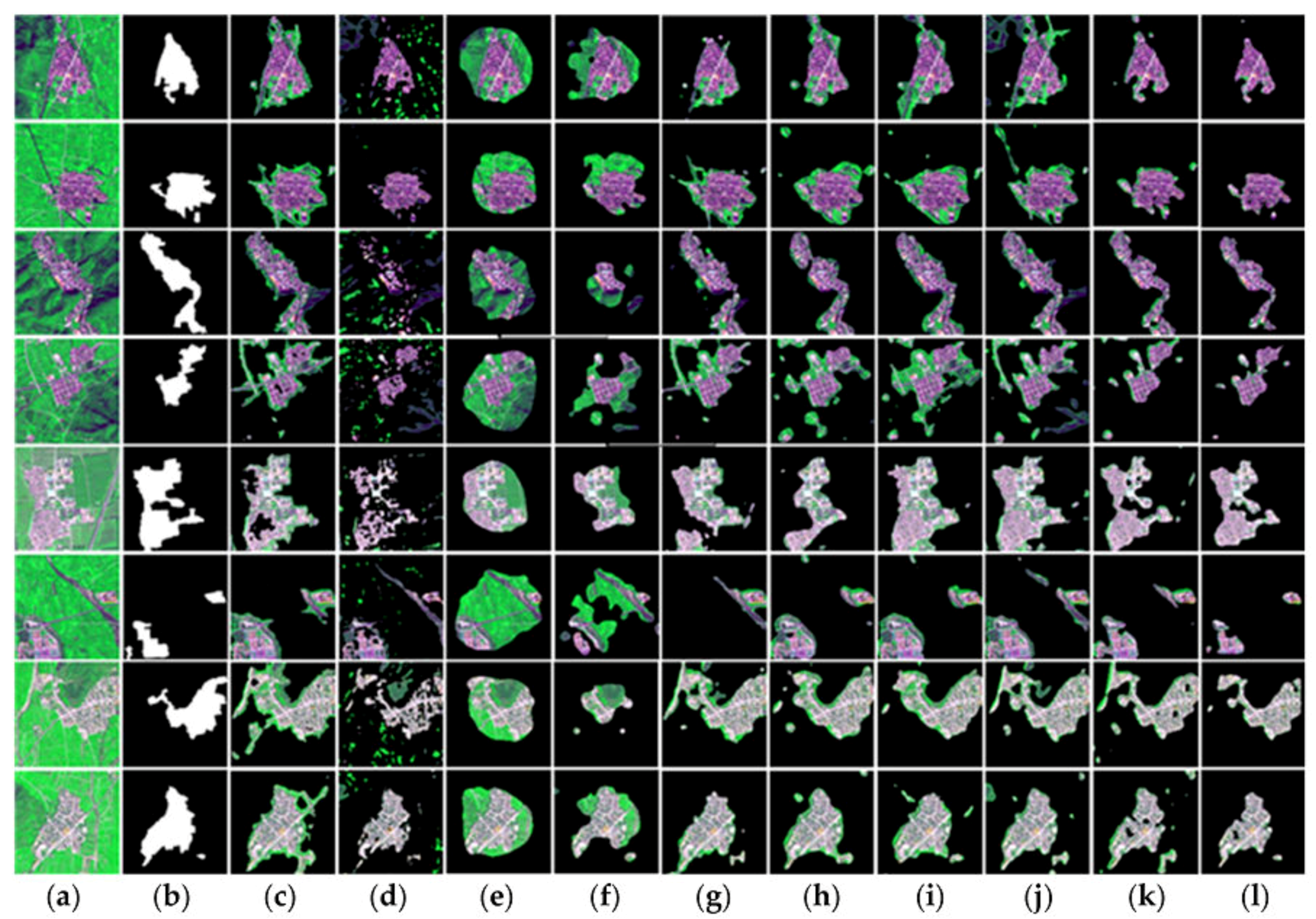
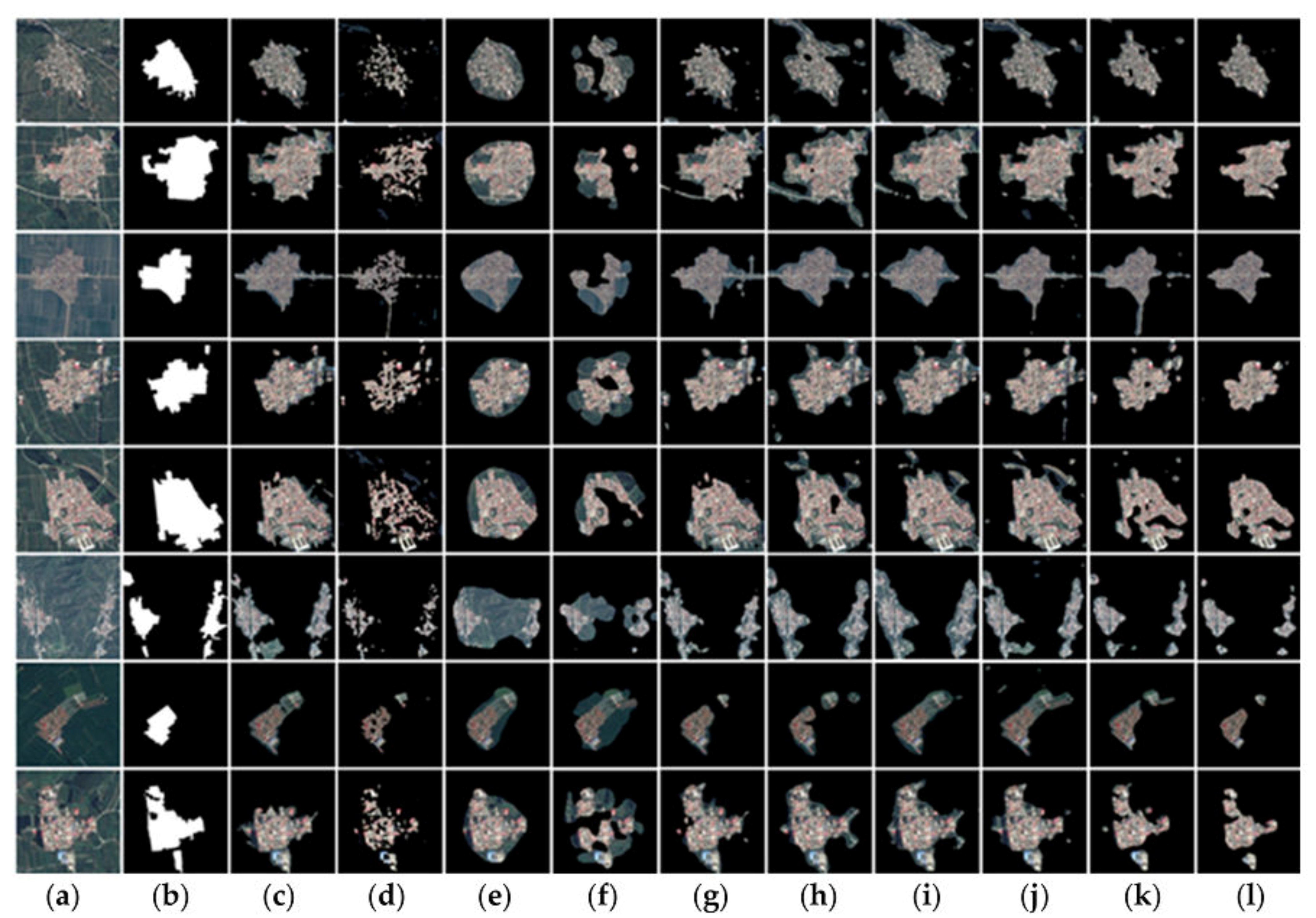
Similarly, we can see the ROIs extraction results for two kinds of images from Figure 7 and Figure 8 after Otsu’s threshold segmentation. For the other nine models, some extracted ROIs are not able to completely contain the residential areas while some ROIs include excessively large redundant background information such as roads, especially in the ROI extraction results of the ITTI model and the GBVS model. In contrast, the proposed model exactly extracts the ROIs with clear boundaries and also has a good performance for remote sensing images with complex background, especially for the images with non-salient regions inside the outline of the residential areas and those with more than one salient region, as is shown in the ROI extraction result on the fifth and sixth images in Figure 7.

On a qualitative level, the experimental results show that the proposed model can not only generate saliency maps with a clear boundary with no excessive redundant background information, but also extracts exactly the ROIs with irregular shape and multi-saliency.

3.2. Quantitative Experiment

In the quantitative analysis of the experiment results, the ROC (Receiver Operator Characteristic) curve is adopted to measure the performance of different models. The ROC curve is derived by thresholding a saliency map at the threshold within the range [0, 255] and further classifying the saliency map into the ROIs and the background. The True Positive Rate (TPR) and the False Positive Rate (FPR) are two dimensions for spanning the ROC curve and respectively denote the percentage of the ROIs from the ground truth intersecting with the ROI from the saliency map and the percentage of the remaining background except for the ROIs. They are both computed as follows:

$$TPR=\frac{{\displaystyle \sum _{i=1}^M}{\displaystyle \sum _{j=1}^N}g\mathit{(}i,j\mathit{)}s\mathit{(}i,j\mathit{)}}{{\displaystyle \sum _{i=1}^M}{\displaystyle \sum _{j=1}^N}g\mathit{(}i,j\mathit{)}}$$

(13)

$$FPR=\frac{{\displaystyle \sum _{i=1}^M}{\displaystyle \sum _{j=1}^N}\mathit{[}1-g\mathit{(}i,j\mathit{)}\mathit{]}s\mathit{(}i,j\mathit{)}}{{\displaystyle \sum _{i=1}^M}{\displaystyle \sum _{j=1}^N}\mathit{[}1-g\mathit{(}i,j\mathit{)}\mathit{]}}$$

(14)

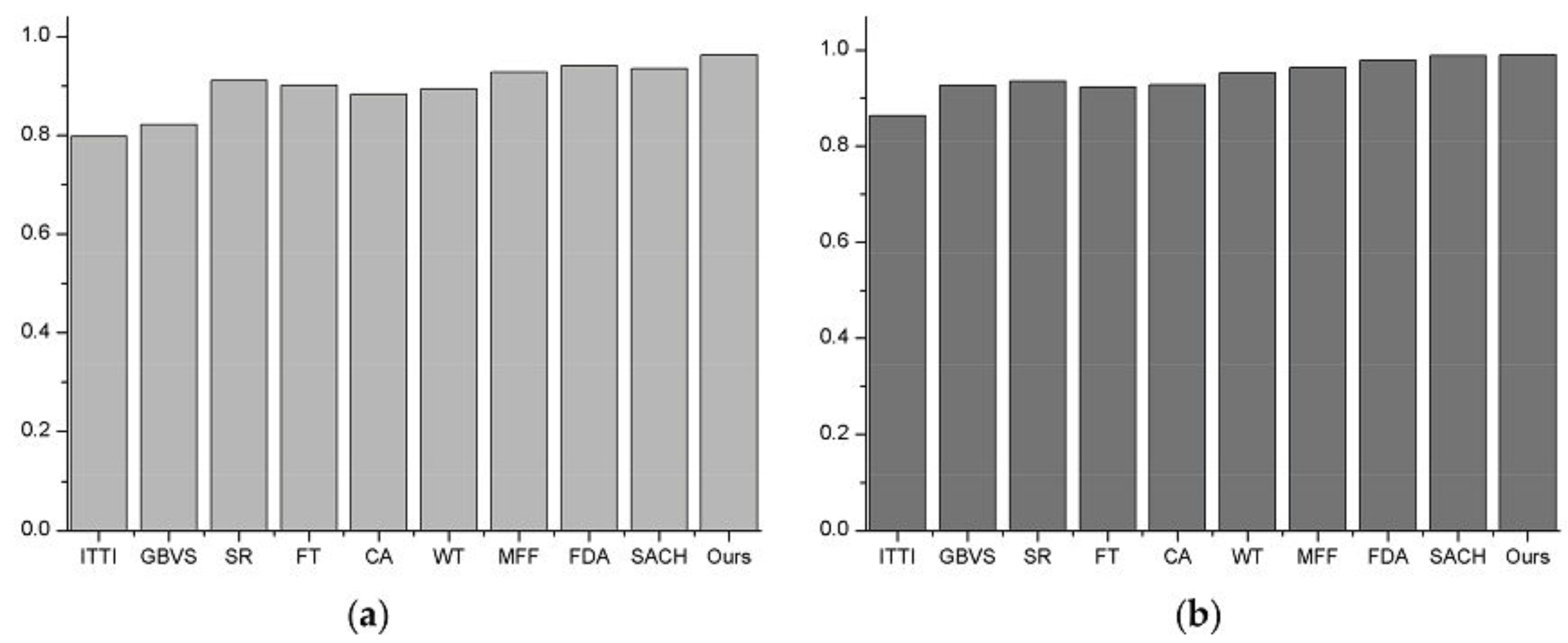
where, for an $M\times N$ image, $g$ denotes the ground truth, $s$ denotes the saliency map after the binary image, and $\mathit{(}i,j\mathit{)}$ denotes the coordinate of the images. A higher TPR value indicates a better performance when the FPR value is the same and, conversely, better performance depends on a smaller FPR value at the same TPR value. The area beneath the curve is called the Area Under the Curve (AUC). Thus, a larger AUC indicates better performance. The AUCs of all the models are shown in

Table 1. The Area Under the Curve (AUC)s of our proposed model and nine competing models on SPOT 5 images.

Model	CA	FT	GBVS	ITTI	WT	SR	MFF	SACH	FDA	OURS
AUC	0.8832	0.9008	0.8216	0.7973	0.8934	0.9107	0.9278	0.9350	0.9408	0.9629

and

Table 2. The AUCs of our proposed model and nine competing models on Google Earth images.

Model	CA	FT	GBVS	ITTI	WT	SR	MFF	SACH	FDA	OURS
AUC	0.9274	0.9227	0.9267	0.8634	0.9531	0.9354	0.9639	0.9889	0.9789	0.9887

. From the Tables we can see that our model obtains the largest value of AUC compared to the other nine competing models, thus achieving better performance.

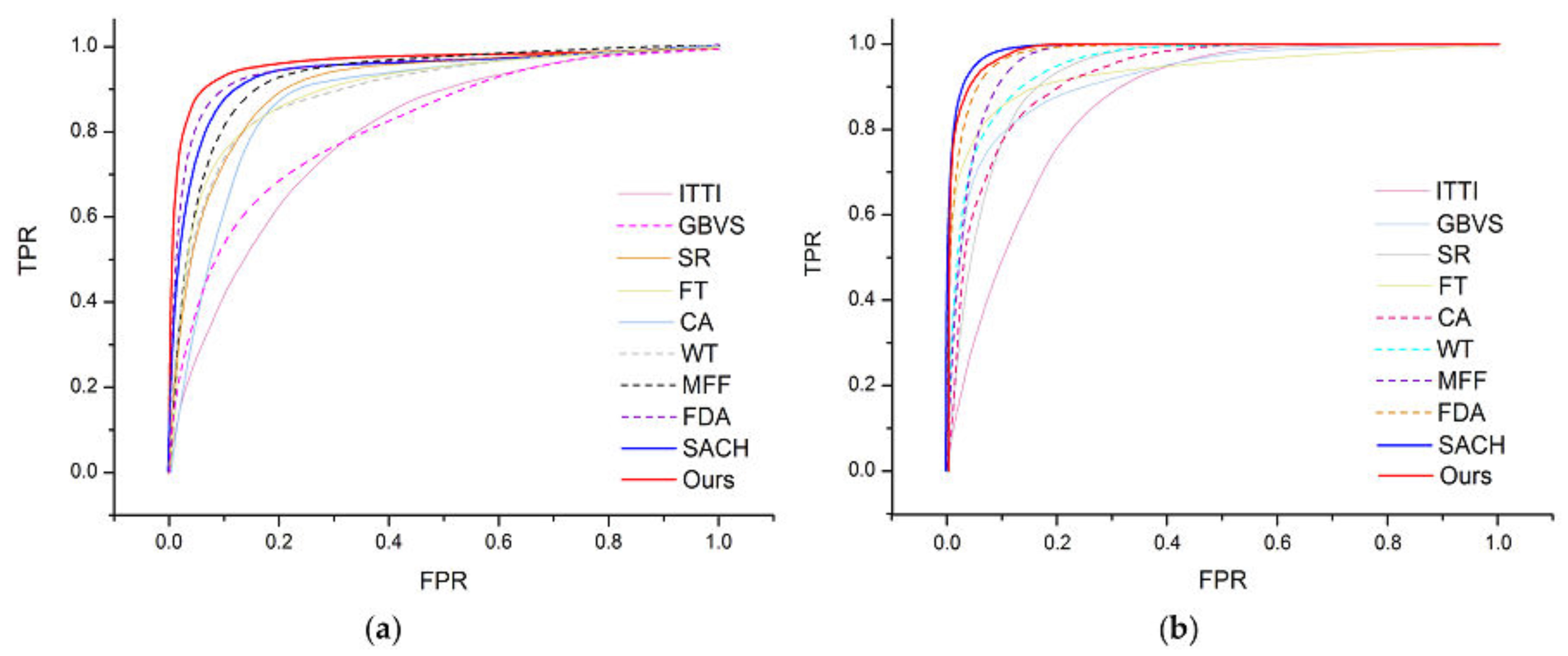
Similarly, we used two kinds of resized remote sensing images of 128 × 128 pixel size to test our model’s performance. For each image, a manually segmented binary map using graphic software was generated as the ground truth. The average TPR and FPR values of every model are computed, and their ROCs on two kinds of images are shown in Figure 9a,b, respectively. From Figure 9a, we can conclude that the ROC curve that our model generated seems to show better performance than the others. However, we can see from Figure 9b that the performance of the SACH model is slightly better than our model whose ROC trace almost coincides with the other one. Therefore, we can know that the same model may have different performance for different kinds of remote sensing images, such as the FDA model and SACH model. The AUC comparison in Figure 10a,b further verifies our conclusion exactly, meanwhile, the Table 1 and Table 2 also show the clear value of AUC.

Another method based on Precision, Recall and the F-Measure which are denoted as P, R and F is also adopted to further evaluate the model’s performance. They are computed as follows and the comparison of different models is shown in Figure 11a,b.

$$P=\frac{{\displaystyle \sum _{x=1}^M}{\displaystyle \sum _{y=1}^N}t\mathit{(}x,y\mathit{)}s\mathit{(}x,y\mathit{)}}{{\displaystyle \sum _{x=1}^M}{\displaystyle \sum _{y=1}^N}s\mathit{(}x,y\mathit{)}}$$

(15)

$$R=\frac{{\displaystyle \sum _{x=1}^M}{\displaystyle \sum _{y=1}^N}t\mathit{(}x,y\mathit{)}s\mathit{(}x,y\mathit{)}}{{\displaystyle \sum _{x=1}^M}{\displaystyle \sum _{y=1}^N}t\mathit{(}x,y\mathit{)}}$$

(16)

$$F_{\beta }=\mathit{(}1+{\beta }^2\mathit{)}\frac{P\cdot R}{{\beta }^2\cdot P+R}$$

(17)

where, for an image with size of $M\times N$, $t\mathit{(}x,y\mathit{)}$ denotes the ground truth, and $s\mathit{(}x,y\mathit{)}$ denotes the saliency map. The $\beta$ serves as an indicator for the relative importance between precision and recall. The larger the value of $\beta$, the more emphasis we put on recall than precision and vice versa. We choose $\beta =1$ to equally balance the weight in our experiment.

From Figure 11a,b the precision of our model is obviously much higher than the other nine competing models, which means our model returns substantially more salient regions than background regions. Based on the previous qualitative analysis, the CA, WT, SR, MFF, SACH and FDA models achieve higher recall than the proposed model, probably because these models capture not only salient areas but some little non-salient regions with blurred boundaries. Meanwhile, this can be obtained clearly and reasonably according to Equation (17). Although the Recall is not the highest among these models, and in Google Earth dataset our ROC curve is slightly worse than SACH, our model still achieves the highest F-measure, thus showing better performance than others on different kinds of remote sensing images.

Additionally, we have compared the computational time for each method using matlab on a PC with 8 G RAM, Intel Core i3-4170 CPU @ 3.70 GHz. For the proposed model, the size of all these images used for learning a dictionary is down-sampled to 128 × 128 pixels. Here, we resized all images to the size of 128 × 128 pixels for fair comparison. From the

Table 3. Running time comparisons for 10 models.

Model	FDA	FT	SR	ITTI	SACH	MFF	GBVS	WT	CA	OURS
AUC	0.85	1.72	2.04	3.68	4.83	6.81	18.43	106.51	1664	5.72

we can see that the run time of our proposed model is in the middle of the ten methods.

The FDA, FT, SR, ITTI and SACH model have a shorter run time than our model. The ITTI, FT and SR model are not proposed for remote sensing images. They do not take into account the complex background of remote sensing images, and use only a few simple features for analysis. The models FDA and SACH are specially designed for remote sensing images. For the former, there remain some holes in ROIs and the latter is not as high as our F-measure evaluation.

The MFF, GBVS, WT and CA model have a longer run time than our model. GBVS generates the final saliency maps of low resolution with blurred boundaries. WT and CA can always get acceptable results some non-salient regions were still extracted. Although MFF does not perform badly, it is not accurate enough.

4. Applications

Because of the development of remote sensing technology, remote sensing image registration and fusion have been paid more and more attention in this field. Some researchers have applied region based image fusion algorithms to remote sensing images [50]. In the previous section, our experiments show that our model can extract ROI accurately from high resolution remote sensing images. Therefore, according to the region information provided by our model and the Gauss Pyramid decomposition, we can obtain more details from different scales of the original images, and then carry out image fusion to construct a clearer and accurate map.

The JPEG 2000 standard demonstrates many attractive features, including the ROI definition. In this case, ROI needs to encode with higher quality than the background [51]. However, knowing how to accurately select investment returns is still a prominent problem. Therefore, the results of our model can also be applied to image compression. The saliency map of the image can be detected and the visual importance [52] of the image pixels is measured, so that ROI can be considered as a step in the process of image compression priority encoding. According to Figure 12, the ROI still has a high subjective quality even at low bit rates (e.g., 0.5 bpp).

5. Conclusions

This paper proposes a novel model based on hyperparameter sparse representation and energy distribution optimizing for saliency analysis and ROI detection in remote sensing images. The proposed model is simple to use and makes up the deficiency of biological plausibility as well as achieving better performance on saliency analysis and ROI detection. In this model, we firstly down-sample the original images and then transform them to HSI color space to increase the efficiency for further processing. After the overlapped patches segmentation and vectorization, a feature learning algorithm is adopted to train the dictionary for sparse representation. Then, energy distribution optimizing based on the principle of predictive coding is used to maximize the entropy of the feature of visual saliency, thereby generating the final saliency map. Finally, ROIs are extracted from original images with Otsu’s segmentation method implemented in the obtained saliency map. Experimental results in two different kinds of remote sensing images demonstrate that the proposed model outperforms the other nine models in ROI extraction, qualitatively and quantitatively. In our experiments, each pixel is simply used as feature and only the number of features need to be chosen. Thus, there is no need to consider the specific structural information of different remote sensing images, which may provide a new unified method for feature extraction for image processing areas such as object compression, segmentation and recognition in the future.