
Archaeological Application of Airborne LiDAR with Object-Based Vegetation Classification and Visualization Techniques at the Lowland Maya Site of Ceibal, Guatemala

 , ,
, ,
Abstract
:
1. Introduction
2. Materials and Methods
2.1. LiDAR Data Acquisition
2.2. Visualization Techniques
2.3. Archaeological Feature Detection in LiDAR Data
2.4. Field Verification of Archaeological Features
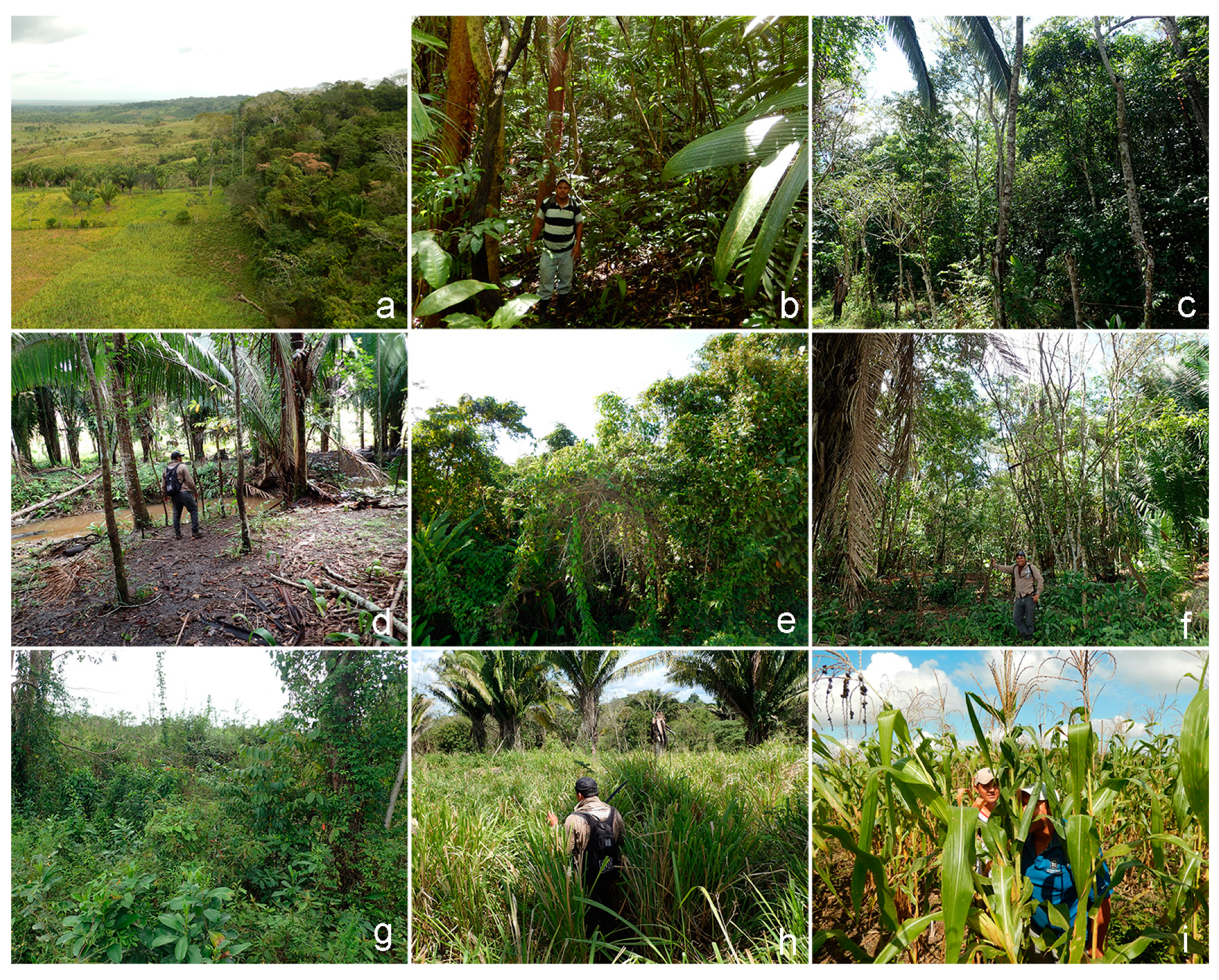
2.5. Vegetation Survey
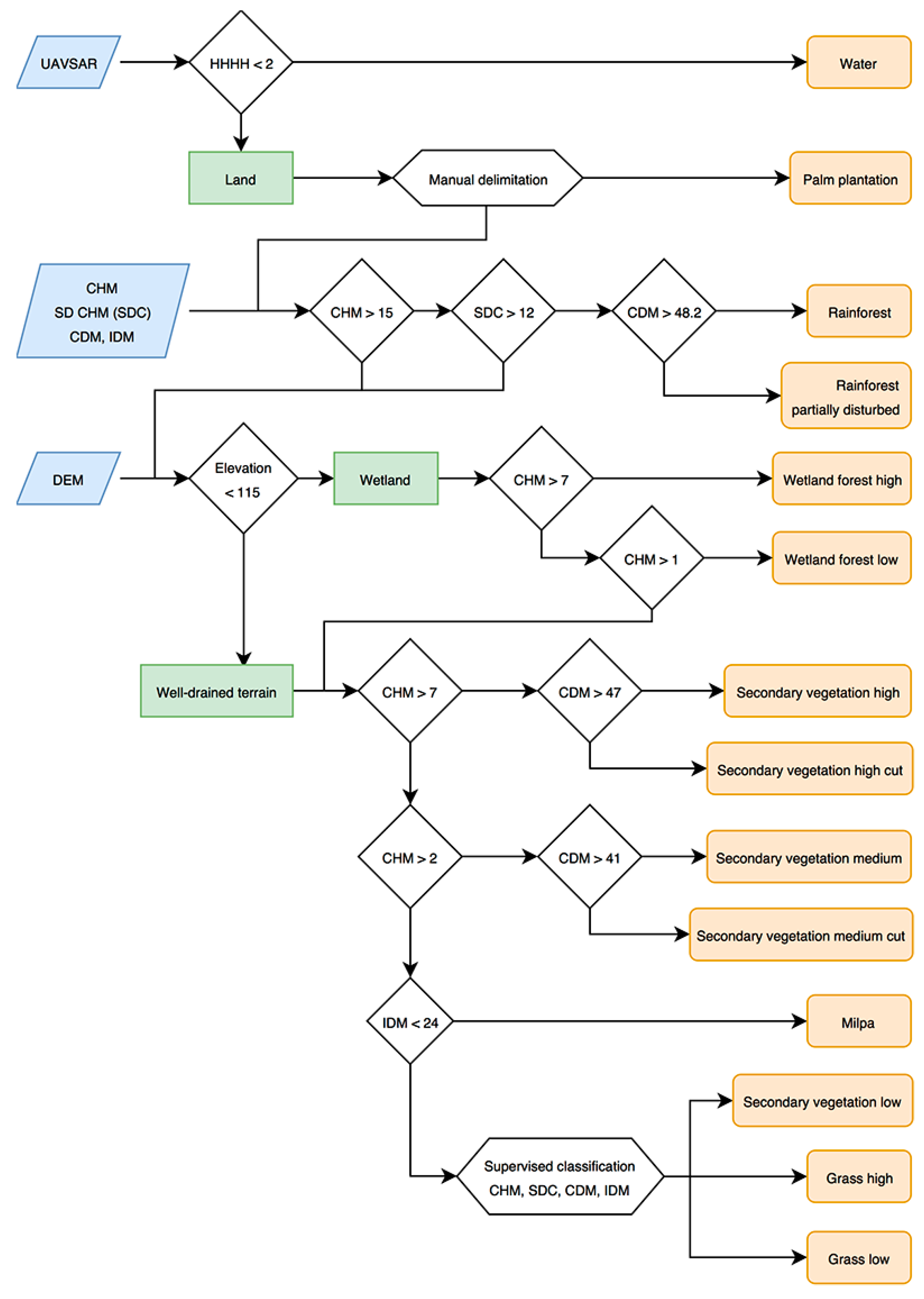
2.6. OBIA Vegetation Classification with LiDAR Data
3. Results
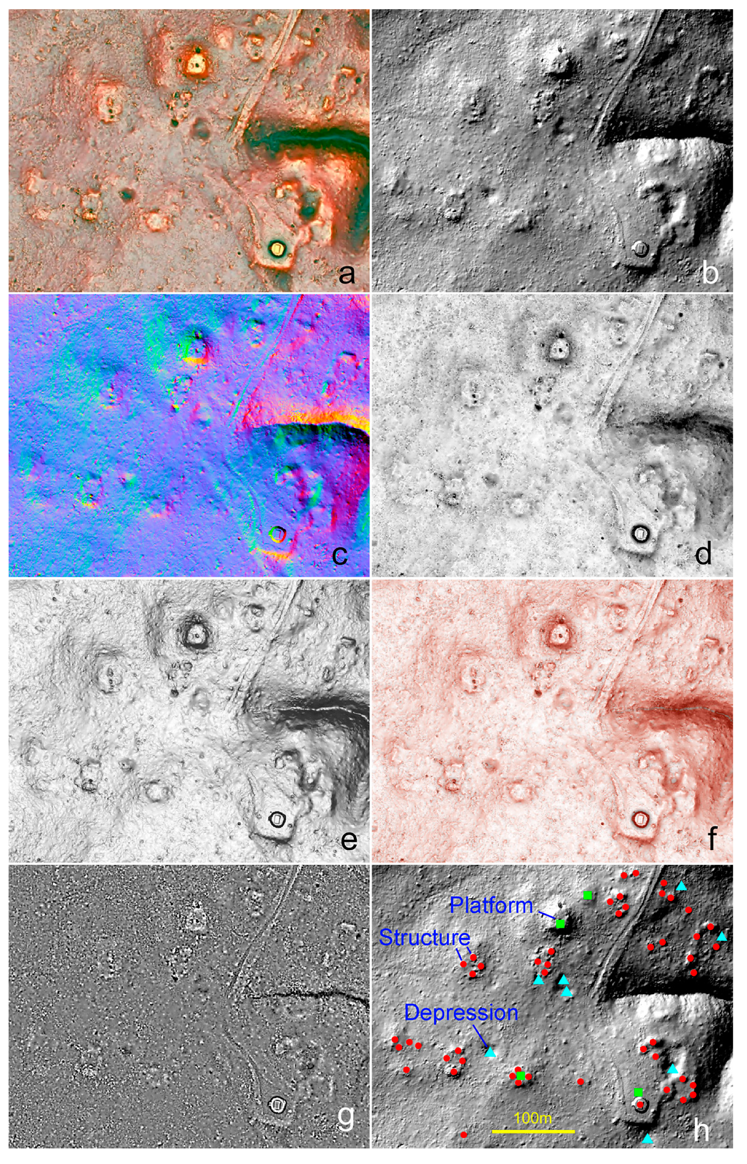
3.1. Comparison of RRIM with Other Visualization Techniques
3.2. Vegetation Classification
3.3. Assessment of Archaeological Features Detection in LiDAR Data
4. Discussion
5. Conclusions
Acknowledgments
Author Contributions
Conflicts of Interest
References
- Chase, A.F.; Chase, D.Z.; Weishampel, J.F.; Drake, J.B.; Shrestha, R.L.; Slatton, K.C.; Awe, J.J.; Carter, W.E. Airborne LiDAR, archaeology, and the ancient Maya landscape at Caracol, Belize. J. Archaeol. Sci. 2011, 38, 387–398. [Google Scholar] [CrossRef]
- Chase, A.F.; Chase, D.; Awe, J.; Weishampel, J.; Iannone, G.; Moyes, H.; Yaeger, J.; Brown, M.K. The use of LiDAR in understanding the Ancient Maya landscape. Adv. Archaeol. Pract. 2014, 2, 208–221. [Google Scholar] [CrossRef]
- Chase, A.F.; Chase, D.Z.; Fisher, C.T.; Leisz, S.J.; Weishampel, J.F. Geospatial revolution and remote sensing LiDAR in Mesoamerican archaeology. Proc. Natl. Acad. Sci. USA 2012, 109, 12916–12921. [Google Scholar] [CrossRef] [PubMed]
- Chase, A.F.; Chase, D.Z.; Awe, J.J.; Weishampel, J.F.; Iannone, G.; Moyes, H.; Yaeger, J.; Brown, M.K.; Shrestha, R.L.; Carter, W.E. Ancient Maya regional settlement and inter-site analysis: The 2013 west-central Belize LiDAR Survey. Remote Sens. 2014, 6, 8671–8695. [Google Scholar] [CrossRef]
- Hare, T.; Masson, M.; Russell, B. High-density LiDAR mapping of the ancient city of Mayapán. Remote Sens. 2014, 6, 9064–9085. [Google Scholar] [CrossRef]
- Golden, C.; Murtha, T.; Cook, B.; Shaffer, D.S.; Schroder, W.; Hermitt, E.J.; Firpi, O.A.; Scherer, A.K. Reanalyzing environmental LiDAR data for archaeology: Mesoamerican applications and implications. J. Archaeol. Sci. Rep. 2016, 9, 293–308. [Google Scholar] [CrossRef]
- Rosenswig, R.M.; López-Torrijos, R.; Antonelli, C.E.; Mendelsohn, R.R. LiDAR mapping and surface survey of the Izapa state on the tropical piedmont of Chiapas, Mexico. J. Archaeol. Sci. 2013, 40, 1493–1507. [Google Scholar] [CrossRef]
- Rosenswig, R.M.; López-Torrijos, R.; Antonelli, C.E. LiDAR data and the Izapa polity: New results and methodological issues from tropical Mesoamerica. Archaeol. Anthropol. Sci. 2015, 7, 487–504. [Google Scholar] [CrossRef]
- Evans, D.H.; Fletcher, R.J.; Pottier, C.; Chevance, J.B.; Soutif, D.; Tan, B.S.; Im, S.; Ea, D.; Tin, T.; Kim, S.; et al. Uncovering archaeological landscapes at Angkor using LiDAR. Proc. Natl. Acad. Sci. USA 2013, 110, 12595–12600. [Google Scholar] [CrossRef] [PubMed]
- Evans, D. Airborne laser scanning as a method for exploring long-term socio-ecological dynamics in Cambodia. J. Archaeol. Sci. 2016, 74, 164–175. [Google Scholar] [CrossRef]
- Hutson, S.R. Adapting LiDAR data for regional variation in the tropics: A case study from the Northern Maya Lowlands. J. Archaeol. Sci. Rep. 2015, 4, 252–263. [Google Scholar] [CrossRef]
- Prufer, K.M.; Thompson, A.E.; Kennett, D.J. Evaluating airborne LiDAR for detecting settlements and modified landscapes in disturbed tropical environments at Uxbenká, Belize. J. Archaeol. Sci. 2015, 57, 1–13. [Google Scholar] [CrossRef]
- Hutson, S.R.; Kidder, B.; Lamb, C.; Vallejo-Cáliz, D.; Welch, J. Small buildings and small budgets: Making LiDAR work in Northern Yucatan, Mexico. Adv. Archaeol. Pract. 2016, 4, 268–283. [Google Scholar] [CrossRef]
- Ebert, C.E.; Hoggarth, J.A.; Awe, J.J. Integrating Quantitative LiDAR analysis and settlement survey in the Belize River Valley. Adv. Archaeol. Pract. 2016, 4, 284–300. [Google Scholar] [CrossRef]
- Reese-Taylor, K.; Hernández, A.A.; Esquivel, A.F.F.; Monteleone, K.; Uriarte, A.; Carr, C.; Acuña, H.G.; Fernandez-Diaz, J.C.; Peuramaki-Brown, M.; Dunning, N. Boots on the ground at Yaxnohcah ground-truthing LiDAR in a complex tropical landscape. Adv. Archaeol. Pract. 2016, 4, 314–338. [Google Scholar] [CrossRef]
- Pingel, T.J.; Clarke, K.; Ford, A. Bonemapping: A LiDAR processing and visualization technique in support of archaeology under the canopy. Cartogr. Geogr. Inf. Sci. 2015, 42, 18–26. [Google Scholar] [CrossRef]
- Magnoni, A.; Stanton, T.W.; Barth, N.; Fernandez-Diaz, J.C.; León, J.F.O.; Ruíz, F.P.; Wheeler, J.A. Detection thresholds of archaeological features in airborne LiDAR data from Central Yucatán. Adv. Archaeol. Pract. 2016, 4, 232–248. [Google Scholar] [CrossRef]
- Bennett, R.; Welham, K.; Ford, A. A comparison of visualization techniques for models created from airborne laser scanned data. Archaeol. Prospect. 2012, 19, 41–48. [Google Scholar] [CrossRef]
- Challis, K.; Forlin, P.; Kincey, M. A generic toolkit for the visualization of archaeological features on airborne LiDAR elevation data. Archaeol. Prospect. 2011, 18, 279–289. [Google Scholar] [CrossRef]
- Devereux, B.J.; Amable, G.S.; Crow, P. Visualisation of LiDAR terrain models for archaeological feature detection. Antiquity 2008, 82, 470. [Google Scholar] [CrossRef]
- Harmon, J.M.; Leone, M.P.; Prince, S.D.; Snyder, M. LiDAR for archaeological landscape analysis: A case study of two eighteenth-century Maryland plantation sites. Am. Antiquity 2006, 71, 649–670. [Google Scholar] [CrossRef]
- Millard, K.; Burke, C.; Stiff, D.; Redden, A. Detection of a low-relief 18th-century British siege trench using LiDAR vegetation penetration capabilities at Fort Beauséjour—Fort Cumberland National Historic Site, Canada. Geoarchaeology 2009, 24, 576–588. [Google Scholar] [CrossRef]
- Štular, B.; Kokalj, Ž.; Oštir, K.; Nuninger, L. Visualization of LiDAR-derived relief models for detection of archaeological features. J. Archaeol. Sci. 2012, 39, 3354–3360. [Google Scholar] [CrossRef]
- Atlas Hidrológico. Available online: http://www.insivumeh.gob.gt/hidrologia/ATLAS_HIDROMETEOROLOGICO/Atlas_Hidrologico/isoyetas.jpg (accessed on 25 November 2016).
- Willey, G.R.; Smith, A.L.; Tourtellot, G., III; Graham, I. Excavations at Seibal, Department of Peten, Guatemala: Introduction: The Site and Its Setting; Harvard University: Cambridge, MA, USA, 1975. [Google Scholar]
- Tourtellot, G., III. Excavations at Seibal, Department of Peten, Guatemala: Peripheral Survey and Excavation, Settlement and Community Patterns; Harvard University: Cambridge, MA, USA, 1988. [Google Scholar]
- Munson, J. Building on the Past: Temple Histories and Communities of Practice at Caobal, Petén, Guatemala. Ph.D. Thesis, University of Arizona, Tucson, AZ, USA, 2012. [Google Scholar]
- Inomata, T.; MacLellan, J.; Triadan, D.; Munson, J.; Burham, M.; Aoyama, K.; Nasu, H.; Pinzon, F.; Yonenobu, H. Development of sedentary communities in the Maya lowlands: Coexisting mobile groups and public ceremonies at Ceibal, Guatemala. Proc. Natl. Acad. Sci. USA 2015, 112, 4268–4273. [Google Scholar] [CrossRef] [PubMed]
- Inomata, T.; Triadan, D.; Aoyama, K.; Castillo, V.; Yonenobu, H. Early ceremonial constructions at Ceibal, Guatemala, and the origins of lowland Maya civilization. Science 2013, 340, 467–471. [Google Scholar] [CrossRef] [PubMed]
- Fernandez-Diaz, J.C.; Carter, W.E.; Shrestha, R.L.; Glennie, C.L. Now you see it… now you don’t: Understanding airborne mapping LiDAR collection and data product generation for archaeological research in Mesoamerica. Remote Sens. 2014, 6, 9951–10001. [Google Scholar] [CrossRef]
- Fernandez-Diaz, J.C.; Carter, W.E.; Glennie, C.; Shrestha, R.L.; Pan, Z.; Ekhtari, N.; Singhania, A.; Hauser, D.; Sartori, M. Capability assessment and performance metrics for the Titan multispectral mapping LiDAR. Remote Sens. 2016, 8, 936. [Google Scholar] [CrossRef]
- Fountain, A.G.; Fernandez-Diaz, J.C.; Levy, J.; Gooseff, M.; Van Horn, D.J.; Morin, P.; Shrestha, R. High-resolution elevation mapping of the McMurdo Dry Valleys, Antarctica and surrounding regions. Earth Syst. Sci. Data 2017. [Google Scholar] [CrossRef]
- LASer (LAS) File Format Exchange Activities. Available online: https://www.asprs.org/committee-general/laser-las-file-format-exchange-activities.html (accessed on 1 February 2017).
- McCoy, M.D.; Asner, G.P.; Graves, M.W. Airborne LiDAR survey of irrigated agricultural landscapes: An application of the slope contrast method. J. Archaeol. Sci. 2011, 38, 2141–2154. [Google Scholar] [CrossRef]
- Pingel, T.; Clarke, K. Perceptually shaded slope maps for the visualization of digital surface models. Cartogr. Int. J. Geogr. Inf. Geovisual. 2014, 49, 225–240. [Google Scholar] [CrossRef]
- Chase, A.S.Z. Beyond Elite Control: Water Management at Caracol. Bachelor’s Thesis, Harvard University, Cambridge, MA, USA, 2012. [Google Scholar]
- Kokalj, Ž.; Zakšek, K.; Oštir, K. Application of sky-view factor for the visualisation of historic landscape features in LiDAR-derived relief models. Antiquity 2011, 85, 263–273. [Google Scholar] [CrossRef]
- Zakšek, K.; Oštir, K.; Kokalj, Ž. Sky-view factor as a relief visualization technique. Remote Sens. 2011, 3, 398–415. [Google Scholar] [CrossRef]
- Chiba, T.; Kaneta, S.; Suzuki, Y. Red relief image map: New visualization method for three dimensional data. Int. Arch. Photogramm. Remote Sens. Spat. Inf. Sci. 2008, 37, 1071–1076. [Google Scholar]
- Chiba, T.; Suzuki, Y. Visualization of airborne laser mapping data: Production and development of red relief image map. Adv. Surv. Technol. 2008, 96, 32–42. (In Japanese) [Google Scholar]
- Yokoyama, R.; Shirasawa, M.; Pike, R.J. Visualizing topography by openness: A new application of image processing to digital elevation models. Photogramm. Eng. Remote Sens. 2002, 68, 257–266. [Google Scholar]
- Sky-View Factor Based Visualization. Available online: http://iaps.zrc-sazu.si/en/svf#v (accessed on 15 January 2017).
- Antonarakis, A.S.; Richards, K.S.; Brasington, J. Object-based land cover classification using airborne LiDAR. Remote Sens. Environ. 2008, 112, 2988–2998. [Google Scholar] [CrossRef]
- Bork, E.W.; Su, J.G. Integrating LiDAR data and multispectral imagery for enhanced classification of rangeland vegetation: A meta analysis. Remote Sens. Environ. 2007, 111, 11–24. [Google Scholar] [CrossRef]
- Lee, A.C.; Lucas, R.M. A LiDAR-derived canopy density model for tree stem and crown mapping in Australian forests. Remote Sens. Environ. 2007, 111, 493–518. [Google Scholar] [CrossRef]
- Millard, K.; Richardson, M. Wetland mapping with LiDAR derivatives, SAR polarimetric decompositions, and LiDAR–SAR fusion using a random forest classifier. Can. J. Remote Sens. 2013, 39, 290–307. [Google Scholar] [CrossRef]
- Naidoo, L.; Cho, M.; Mathieu, R.; Asner, G. Classification of savanna tree species, in the Greater Kruger National Park region, by integrating hyperspectral and LiDAR data in a random forest data mining environment. ISPRS J. Photogramm. Remote Sens. 2012, 69, 167–179. [Google Scholar] [CrossRef]
- Van Leeuwen, M.; Nieuwenhuis, M. Retrieval of forest structural parameters using LiDAR remote sensing. Eur. J. For. Res. 2010, 129, 749–770. [Google Scholar] [CrossRef]
- Liu, X.; Li, Y.; Gao, W.; Xiao, L. Double polarization SAR image classification based on object-oriented technology. J. Geogr. Inf. Syst. 2010, 2, 113. [Google Scholar] [CrossRef]
- Ryherd, S.; Woodcock, C. Combining spectral and texture data in the segmentation of remotely sensed images. Photogramm. Eng. Remote Sens. 1996, 62, 181–194. [Google Scholar]
- Syed, S.; Dare, P.; Jones, S. Automatic classification of land cover features with high resolution imagery and LiDAR data: An object-oriented approach. In Proceedings of the SSC2005 Spatial Intelligence, Innovation and Praxis: The National Biennial Conference of the Spatial Sciences Institute, September 2005; Spatial Sciences Institute: Melbourne, Auatralia, 2005; pp. 512–522. [Google Scholar]
- Verhagen, P.; Drăguţ, L. Object-based landform delineation and classification from DEMs for archaeological predictive mapping. J. Archaeol. Sci. 2012, 39, 698–703. [Google Scholar] [CrossRef]
- UAVSAR. Available online: https://uavsar.jpl.nasa.gov/cgi-bin/product.pl?jobName=Aguatc_03901_10014_009_100202_L090_CX_01#data (accessed on 1 October 2016).
- UAVSAR. Available online: https://uavsar.jpl.nasa.gov/cgi-bin/product.pl?jobName=Aguatc_31602_10014_011_100202_L090_CX_01#data (accessed on 1 October 2016).
- AIRSAR. Available online: https://airsar.asf.alaska.edu/data/ts/ts1789/ (accessed on 1 October 2016).
- Brennan, R.; Webster, T.L. Object-oriented land cover classification of LiDAR-derived surfaces. Can. J. Remote Sens. 2006, 32, 162–172. [Google Scholar] [CrossRef]
- Kim, S.b.; Ouellette, J.D.; van Zyl, J.J.; Johnson, J.T. Detection of inland open water surfaces using dual polarization L-band radar for the soil moisture active passive mission. IEEE Trans. Geosci. Remote Sens. 2016, 54, 3388–3399. [Google Scholar] [CrossRef]
- Matgen, P.; Hostache, R.; Schumann, G.; Pfister, L.; Hoffmann, L.; Savenije, H.H.G. Towards an automated SAR-based flood monitoring system: Lessons learned from two case studies. Phys. Chem. Earth Parts A/B/C 2011, 36, 241–252. [Google Scholar] [CrossRef]
- Giustarini, L.; Hostache, R.; Matgen, P.; Schumann, G.J.; Bates, P.D.; Mason, D.C. A change detection approach to flood mapping in urban areas using TerraSAR-X. IEEE Trans. Geosci. Remote. Sens. 2013, 51, 2417–2430. [Google Scholar] [CrossRef]
- Henry, J.B.; Chastanet, P.; Fellah, K.; Desnos, Y.L. Envisat multi-polarized ASAR data for flood mapping. Int. J. Remote Sens. 2006, 27, 1921–1929. [Google Scholar] [CrossRef]
- Lin, Z.; Kaneda, H.; Mukoyama, S.; Asada, N.; Chiba, T. Detection of subtle tectonic–geomorphic features in densely forested mountains by very high-resolution airborne LiDAR survey. Geomorphology 2013, 182, 104–115. [Google Scholar] [CrossRef]
- Razak, K.A.; Straatsma, M.W.; Van Westen, C.J.; Malet, J.; De Jong, S.M. Airborne laser scanning of forested landslides characterization: Terrain model quality and visualization. Geomorphology 2011, 126, 186–200. [Google Scholar] [CrossRef]
- Zielke, O.; Klinger, Y.; Arrowsmith, J.R. Fault slip and earthquake recurrence along strike-slip faults—Contributions of high-resolution geomorphic data. Tectonophysics 2015, 638, 43–62. [Google Scholar] [CrossRef]
- Shimoda, I.; Haraguchi, T.; Chiba, T.; Shimoda, M. The advanced hydraulic city structure of the royal city of Angkor Thom and vicinity revealed through a high-resolution Red Relief Image Map. Archaeol. Discov. 2015, 4, 22. [Google Scholar]


| Dataset | Acquisition | Horizontal Resolution | Coverage | Use |
|---|---|---|---|---|
| LiDAR-derived Canopy Density Model (CDM) | 2015 | 4 m | 441 km2 | OBIA (Classification of dense and sparse vegetation) |
| LiDAR-derived window averaged Canopy Height Model (CHM) | 2015 | 4 m | 441 km2 | OBIA (Vegetation classification by height) |
| LiDAR-derived window standard deviation of CHM (SD CHM) | 2015 | 4 m | 441 km2 | OBIA (Separation of rainforest and secondary vegetation) |
| LiDAR-derived Intensity Difference Model (IDM) | 2015 | 4 m | 441 km2 | OBIA (Primarily the identification of agricultural fields) |
| LiDAR-derived DEM | 2015 | 0.5 m | 460 km2 | OBIA (Delineation of wetlands) |
| Uninhabited Aerial Vehicle Synthetic Aperture Radar (UAVSAR) | 2010 | 6 m | 1637 km2 (439 km2 of the LiDAR area) | OBIA (Delineation of water) |
| IKONOS | 2006 and 2007 | 4 m (red, green, blue, and NIR) and 1 m (panchromatic) | 104 km2 within the LiDAR area | Previous studies and occasional comparison with OBIA |
| Orthophotos | 2006 | 0.5 m | Entire LiDAR area | Previous studies and occasional comparison with OBIA |
| Airborne Synthetic Aperture Radar (AIRSAR) | 2004 | 5 m | 452 km2 (254 km2 of the LiDAR area) | Previous studies |
| Landsat 7 and 8 | Multiple dates | 30 m for most bands | Entire LiDAR area | Previous studies |
| Techniques | Structures | Platforms | Depressions |
|---|---|---|---|
| Harvard map | 44 | N/A | N/A |
| RRIM | 49 | 4 | 8 |
| Hillshade | 46 | 4 | 8 |
| PCA | 46 | 4 | 8 |
| SVF | 35 | 3 | 8 |
| Slope gradient | 45 | 4 | 7 |
| SVF + Slope g. | 45 | 4 | 8 |
| Moving-window ED | 34 | 2 | 8 |
| Vegetation Type | Note | Area (km2) | CHM (m) 1 | STD CHM 1 | CDM 1 | IDM 1 | ||||
|---|---|---|---|---|---|---|---|---|---|---|
| Mean | S.d. | Mean | S.d. | Mean | S.d. | Mean | S.d. | |||
| Rainforest | 23.30 | 21.56 | 6.90 | 18.67 | 6.30 | 48.89 | 1.91 | 29.88 | 4.00 | |
| Rainforest partially disturbed | 1.88 | 16.86 | 6.69 | 20.11 | 6.82 | 46.75 | 5.10 | 29.02 | 4.27 | |
| Secondary vegetation high | 12 to 30 years old. Includes disturbed rainforest. | 25.11 | 11.16 | 5.03 | 11.99 | 5.58 | 47.58 | 4.53 | 28.51 | 3.40 |
| Secondary vegetation high cut | Includes reforested areas. | 4.83 | 9.07 | 5.26 | 14.21 | 7.01 | 41.20 | 9.96 | 26.99 | 4.79 |
| Secondary vegetation medium | 3 to 15 years old. | 26.39 | 4.25 | 2.70 | 6.68 | 3.43 | 44.82 | 6.13 | 26.94 | 2.75 |
| Secondary vegetation medium cut | Includes reforested areas, orchards, cohune palm forests, and settlements with trees. | 21.03 | 3.10 | 3.62 | 9.81 | 5.59 | 27.45 | 12.97 | 24.37 | 4.96 |
| Secondary vegetation low | 1 to 10 years old. Includes very dense vegetation without LiDAR penetration and wetland grass. | 31.27 | 0.87 | 1.28 | 2.81 | 2.90 | 35.35 | 9.08 | 25.40 | 1.87 |
| Grass high | Includes 1 year old recovery vegetation, densely covered agricultural fields, and wetland grass. | 50.51 | 0.41 | 1.17 | 2.10 | 3.17 | 23.51 | 8.35 | 25.42 | 1.73 |
| Grass low | Includes pasture, agricultural fields with low plants, and wetland grass. | 172.61 | 0.37 | 1.38 | 2.33 | 3.86 | 12.77 | 8.47 | 25.55 | 2.10 |
| Milpa | Includes maize fields and open grounds. | 6.73 | 0.72 | 1.30 | 2.60 | 3.43 | 24.06 | 8.88 | 21.42 | 3.95 |
| Palm plantation | 10.67 | 0.47 | 1.48 | 1.60 | 3.16 | 22.74 | 11.05 | 25.77 | 1.44 | |
| Wetland forest high | 17.02 | 8.86 | 3.76 | 9.17 | 4.74 | 47.45 | 3.78 | 27.72 | 2.47 | |
| Wetland forest low | 43.82 | 4.09 | 2.87 | 6.20 | 3.60 | 44.29 | 8.38 | 26.29 | 2.09 | |
| Water | 6.16 | 0.62 | 2.27 | 2.69 | 5.48 | 7.36 | 14.38 | 25.43 | 1.02 | |
| Area | Shots/m2 | Return/m2 | Ground Return/m2 | Returns/Shot | Ground Return/Shot | Ground Return/Return |
|---|---|---|---|---|---|---|
| Vegetation Type | ||||||
| Areas without test flights | ||||||
| Rainforest | 17.04 | 26.34 | 0.56 | 1.55 | 3.3% | 2.1% |
| Rainforest partially disturbed | 17.35 | 27.49 | 1.64 | 1.58 | 9.4% | 6.0% |
| Secondary vegetation high | 15.87 | 23.34 | 1.09 | 1.47 | 6.9% | 4.7% |
| Secondary vegetation high cut | 15.94 | 24.07 | 3.91 | 1.51 | 24.5% | 16.2% |
| Secondary vegetation medium | 16.98 | 23.06 | 2.35 | 1.36 | 13.9% | 10.2% |
| Secondary vegetation medium cut | 17.47 | 22.20 | 8.87 | 1.27 | 50.8% | 40.0% |
| Secondary vegetation low | 18.83 | 20.58 | 5.83 | 1.09 | 30.9% | 28.3% |
| Grass high | 19.47 | 19.99 | 10.10 | 1.03 | 51.9% | 50.5% |
| Grass low | 18.21 | 18.37 | 12.79 | 1.01 | 70.2% | 69.6% |
| Milpa | 19.06 | 23.06 | 11.14 | 1.21 | 58.4% | 48.3% |
| Palm plantation | 17.99 | 18.58 | 8.67 | 1.03 | 48.2% | 46.6% |
| Wetland forest high | 17.61 | 24.43 | 1.19 | 1.39 | 6.8% | 4.9% |
| Wetland forest low | 17.59 | 21.78 | 2.19 | 1.24 | 12.4% | 10.0% |
| Areas with test flights | ||||||
| Rainforest | 68.58 | 126.23 | 2.84 | 1.84 | 4.1% | 2.3% |
| Rainforest partially disturbed | 72.13 | 134.17 | 8.02 | 1.86 | 11.1% | 6.0% |
| Secondary vegetation high | 61.80 | 104.78 | 7.12 | 1.70 | 11.5% | 6.8% |
| Secondary vegetation high cut | 56.87 | 109.93 | 19.49 | 1.93 | 34.3% | 17.7% |
| Secondary vegetation medium cut | 51.84 | 61.93 | 27.62 | 1.19 | 53.3% | 44.6% |
| Secondary vegetation low | 67.45 | 71.85 | 19.55 | 1.07 | 29.0% | 27.2% |
| Grass high | 62.52 | 68.76 | 35.26 | 1.10 | 56.4% | 51.3% |
| Grass low | 64.37 | 68.41 | 42.48 | 1.06 | 66.0% | 62.1% |
| Milpa | 58.87 | 76.67 | 27.17 | 1.30 | 46.2% | 35.4% |
| Wetland forest high | 68.45 | 104.12 | 3.62 | 1.52 | 5.3% | 3.5% |
| Wetland forest low | 70.17 | 88.19 | 7.30 | 1.26 | 10.4% | 8.3% |
| Area | LiDAR Analysis | Ground-Truthing 1 | Accuracy 1 | ||||||
|---|---|---|---|---|---|---|---|---|---|
| Identification | Count | Tar. | Pos. | Dis. | Field | Det. | Fal. | Fal. | |
| Ver. | Ver. | IDed | Acc. | Pos. | Neg. | ||||
| Vegetation Type | |||||||||
| Areas without test flights (low point density) | |||||||||
| Rainforest | Structure | 950 | 49 | 48 | 1 | 22 | 69% | 1% | 31% |
| Possible str. | 717 | 6 | 6 | 100% | 0% | 0% | |||
| Rainforest partially disturbed | Structure | 27 | 10 | 9 | 1 | 3 | 75% | 8% | 25% |
| Possible str. | 30 | ||||||||
| Secondary vegetation high | Structure | 440 | 41 | 39 | 2 | 17 | 70% | 4% | 30% |
| Possible str. | 281 | 5 | 3 | 2 | 100% | 67% | 0% | ||
| Secondary vegetation high cut | Structure | 97 | 13 | 13 | 3 | 81% | 0% | 19% | |
| Possible str. | 50 | 6 | 6 | 100% | 0% | 0% | |||
| Secondary vegetation medium | Structure | 171 | 10 | 10 | 100% | 0% | 0% | ||
| Possible str. | 156 | ||||||||
| Secondary vegetation medium cut | Structure | 608 | 67 | 62 | 5 | 10 | 86% | 7% | 14% |
| Possible str. | 263 | 11 | 5 | 6 | 100% | 120% | 0% | ||
| Secondary vegetation low | Structure | 227 | 24 | 24 | 100% | 0% | 0% | ||
| Possible str. | 215 | 2 | 2 | 100% | 0% | 0% | |||
| Grass high | Structure | 629 | 40 | 40 | 13 | 75% | 0% | 25% | |
| Possible str. | 303 | 9 | 6 | 3 | 100% | 50% | 0% | ||
| Grass low | Structure | 5336 | 519 | 497 | 22 | 88 | 85% | 4% | 15% |
| Possible str. | 1878 | 72 | 46 | 26 | 100% | 57% | 0% | ||
| Milpa | Structure | 493 | 20 | 20 | 7 | 74% | 0% | 26% | |
| Possible str. | 181 | 2 | 2 | 100% | 0% | 0% | |||
| Palm plantation | Structure | 157 | |||||||
| Possible str. | 142 | ||||||||
| Wetland forest high | Structure | 0 | |||||||
| Possible str. | 0 | ||||||||
| Wetland forest low | Structure | 0 | |||||||
| Possible str. | 2 | ||||||||
| Outside the classified area | Structure | 573 | 7 | 7 | 7 | 50% | 0% | 50% | |
| Possible str. | 155 | 1 | 1 | 100% | 0% | 0% | |||
| Areas with test flights (high point density) | |||||||||
| Rainforest | Structure | 407 | 13 | 12 | 1 | 2 | 86% | 7% | 14% |
| Possible str. | 154 | 1 | 1 | 100% | 0% | 0% | |||
| Rainforest partially disturbed | Structure | 18 | 1 | 1 | 100% | 0% | 0% | ||
| Secondary vegetation high | Structure | 14 | 9 | 9 | 100% | 0% | 0% | ||
| Secondary vegetation medium cut | Structure | 6 | 5 | 5 | 100% | 0% | 0% | ||
| Possible str. | 1 | ||||||||
| Secondary vegetation low | Structure | 5 | 4 | 4 | 100% | 0% | 0% | ||
| Possible str. | 2 | ||||||||
| Grass high | Structure | 28 | 21 | 21 | 100% | 0% | 0% | ||
| Possible str. | 3 | ||||||||
| Grass low | Structure | 12 | 5 | 4 | 1 | 1 | 80% | 20% | 20% |
| Milpa | Structure | 10 | 8 | 8 | 2 | 80% | 0% | 20% | |
| Possible str. | 5 | ||||||||
© 2017 by the authors. Licensee MDPI, Basel, Switzerland. This article is an open access article distributed under the terms and conditions of the Creative Commons Attribution (CC BY) license (http://creativecommons.org/licenses/by/4.0/).
Share and Cite
Inomata, T.; Pinzón, F.; Ranchos, J.L.; Haraguchi, T.; Nasu, H.; Fernandez-Diaz, J.C.; Aoyama, K.; Yonenobu, H. Archaeological Application of Airborne LiDAR with Object-Based Vegetation Classification and Visualization Techniques at the Lowland Maya Site of Ceibal, Guatemala. Remote Sens. 2017, 9, 563. https://doi.org/10.3390/rs9060563
Inomata T, Pinzón F, Ranchos JL, Haraguchi T, Nasu H, Fernandez-Diaz JC, Aoyama K, Yonenobu H. Archaeological Application of Airborne LiDAR with Object-Based Vegetation Classification and Visualization Techniques at the Lowland Maya Site of Ceibal, Guatemala. Remote Sensing. 2017; 9(6):563. https://doi.org/10.3390/rs9060563
Chicago/Turabian StyleInomata, Takeshi, Flory Pinzón, José Luis Ranchos, Tsuyoshi Haraguchi, Hiroo Nasu, Juan Carlos Fernandez-Diaz, Kazuo Aoyama, and Hitoshi Yonenobu. 2017. "Archaeological Application of Airborne LiDAR with Object-Based Vegetation Classification and Visualization Techniques at the Lowland Maya Site of Ceibal, Guatemala" Remote Sensing 9, no. 6: 563. https://doi.org/10.3390/rs9060563
APA StyleInomata, T., Pinzón, F., Ranchos, J. L., Haraguchi, T., Nasu, H., Fernandez-Diaz, J. C., Aoyama, K., & Yonenobu, H. (2017). Archaeological Application of Airborne LiDAR with Object-Based Vegetation Classification and Visualization Techniques at the Lowland Maya Site of Ceibal, Guatemala. Remote Sensing, 9(6), 563. https://doi.org/10.3390/rs9060563