Article

A Novel Spectral Library Pruning Technique for Spectral Unmixing of Urban Land Cover

1
Division of Forest, Nature and Landscape, KU Leuven, Leuven 3001, Belgium
2
Geography Department, Humboldt-Universität zu Berlin, Berlin 10099, Germany
3
Flemish Institute for Technological Research, Center for Remote Sensing and Earth Observation Processes (VITO-TAP), Mol 2400, Belgium
*
Author to whom correspondence should be addressed.
Remote Sens. 2017, 9(6), 565; https://doi.org/10.3390/rs9060565
Submission received: 24 April 2017 / Revised: 19 May 2017 / Accepted: 31 May 2017 / Published: 6 June 2017

Abstract

:
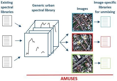
Spectral unmixing of urban land cover relies on representative endmember libraries. For repeated mapping of multiple cities, the use of a generic spectral library, capturing the vast spectral variability of urban areas, would constitute a more operational alternative to the tedious development of image-specific libraries prior to mapping. The size and heterogeneity of such a generic library requires an efficient pruning technique to extract site-specific spectral libraries. We propose the “Automated MUsic and spectral Separability based Endmember Selection technique” (AMUSES), which selects endmember subsets with respect to the image to be processed, while accounting for internal redundancy. Experiments on simulated hyperspectral data from Brussels (Belgium) showed that AMUSES selects more relevant endmembers compared to the conventional Iterative Endmember Selection (IES) approach. This ultimately improved mapping results (kappa increased from 0.71 to 0.83). Experiments on real HyMap data from Berlin (Germany) using a combination of libraries from different cities underlined the potential of AMUSES for handling libraries with increasing levels of generality (RMSE decreased from 0.18 to 0.15, while only using 55% of the number of spectra compared to IES). Our findings contribute to the value of generic spectral databases in the development of efficient urban mapping workflows.

Graphical Abstract

1. Introduction

The increasing availability of hyperspectral data from airborne, but especially from upcoming satellite platforms, e.g., EnMAP [1] and HyspIRI [2], presents unprecedented potential for detailed and repeated mapping of urban areas all around the globe. In order to deal with the high spatial and spectral heterogeneity typically present in these environments [3], spectral unmixing approaches are generally required for mapping urban land cover. In spectral unmixing, mixed pixels are modelled as combinations of pure material spectra (or endmembers) to retrieve subpixel land cover fractions. Examples include Multiple Endmember Spectral Mixture Analysis (MESMA [4]), the Monte Carlo Spectral Unmixing model (AutoMCU [5]), Bayesian Spectral Mixture Analysis (BSMA [6]) and sparse unmixing [7]. These algorithms typically rely on spectral libraries, i.e., collections of pure material spectra, to capture the large spectral variability in urban areas. Gathering endmember spectra, either based on field measurements or through the use of supervised or unsupervised image endmember extraction techniques (see [8] for a full overview), remains a tedious and challenging step to be done prior to unmixing. As the quality of the spectral library is key to the success of the unmixing procedure [4], this initial library is often further optimized, i.e., a library subset is selected that optimally represents the endmember variability in the specific image to be processed. This library pruning step has been shown to increase both the computational efficiency (less spectra to be processed) and the accuracy (less spectral confusion) of the subsequent unmixing analysis [9,10].
Building image-specific spectral libraries is a time-consuming process, as it ideally needs to be repeated for each individual image. However, to efficiently process the vast amounts of data gathered using existing and future sensors, there is a clear need for more operational and universally applicable processing algorithms. New strategies are required to optimally make use of the wealth of spectral information already collected. In recent years, multiple urban spectral libraries have been collected using various sensors, at different spatial resolutions, for various cities and on different moments throughout the year (e.g., [11] and all references mentioned therein, [12,13,14,15,16]). All this information merged together in one vast generic urban spectral library would theoretically capture all possible endmember variability present within an urban image, and could consequently be used to process imagery from different study sites, sensors and timings, including those for which previously no endmember information has been extracted. It has already been shown that combining spectral information from multiple resolutions [17] and timings [18] can potentially increase mapping accuracies. From an operational perspective, the main problem arising from such a generic library approach would be its large size and the high share of irrelevant spectra with regard to any individual image. In order for this approach to become a viable alternative to image-specific library creation, there is a clear need for an efficient library pruning algorithm, which would automatically select a small but relevant subset from the generic spectral library for each image to be processed.
Library pruning constitutes an essential part in efficient and universal urban mapping workflows. Today, a wide array of different library pruning techniques already exists. The first set of methods are library-based approaches, which produce an image-independent library subset by identifying and removing library entries that can be modelled by a combination of other library spectra. Examples include EAR [19], CoB [20], MASA [21] and IES [22]. Library-based approaches produce one optimized set of endmembers for an entire image, which, in a complex and heterogeneous urban environment, may result in quite large libraries containing a high fraction of locally irrelevant spectra (e.g., there is no need for a large variety of roof spectra when classifying an urban park).
In response to this, Garcia-Haro et al. [23] launched the idea of using a-priori classification results to subdivide the image in different regions and subsequently steer the pruning process locally based on the assigned classes. Many of these local pruning approaches have been proposed for urban areas, either based on external data [24], a hierarchical MESMA approach [12] or other classification techniques such as support vector machines [25] and object-based segmentation [10,26]. Although successfully increasing the local efficiency and accuracy of the unmixing process, these techniques are not optimized to deal with high amounts of irrelevant spectra typically found in generic spectral libraries. Indeed, knowing a certain area of the image is dominated by vegetation does not enable one to separate relevant from irrelevant vegetation spectra.
A final group of library pruning approaches directly compares candidate endmembers with image spectra, which makes these image-based pruning techniques conceptually the most promising group to deal with generic spectral libraries. Fan and Deng [27] proposed SASD-MESMA, which first selects the best candidate endmembers for each individual pixel based on both spectral angle and spectral distance measures before entering the unmixing stage. Chen et al. [28] apply a similar concept but use sparse unmixing rather than spectral similarity measures during the pruning step. Given the size of a generic spectral library, in combination with the high number of pixels within (especially high resolution) imagery, adopting a pixel-wise library pruning strategy may prove to be computationally inefficient. The MUSIC pruning algorithm (referred hereinafter as “MUSIC-PA”) of Iordache et al. [9], conceptually based on the multiple signal classification algorithm [29,30], successfully avoids this potential drawback by operating on the entire image at once. The algorithm does so by representing the original image as a small set of eigenvectors and subsequently calculating the distance from each library entry to this simplified representation. MUSIC-PA has already been successfully applied on both simulated and real hyperspectral datasets of mainly semi-natural environments (i.e., citrus orchards) and has been shown to increase the accuracy and computational efficiency of subpixel fraction mapping using sparse unmixing [9]. However, during our first experiences with MUSIC-PA in more complex, urban environments we identified remaining redundancies in the final spectral libraries and revealed potential room for improvement [31].
The overarching goal of this study is to demonstrate the complementary strength of the three main library pruning approaches (library-, location- and image-based) for unmixing urban land cover, specifically in the framework of a generic library approach. Therefore, we created a new library pruning algorithm called AMUSES (Automated MUsic and spectral Separability based Endmember Selection), in which the original MUSIC-PA is extended with a spectral separability measure and implemented as a local pruning algorithm. In this study, AMUSES’ ability to cope with spectrally challenging urban land cover types is tested. More specifically, we considered six urban land cover types, i.e., roof, pavement, soil, non-woody vegetation (e.g., grass, crops), woody vegetation (trees and shrubs) and water, which are characterized by a high within-class variability and a low between-class separability [14]. Although challenging, mapping urbanized land into these classes plays an important role in urban environmental research and urban planning [32,33].
Using simulated and real hyperspectral datasets of different sensors and resolutions, we specifically wanted to (1) compare the performance of AMUSES with a more conventional, library-based pruning technique (IES) and the original MUSIC-PA; and (2) test the potential of AMUSES for dealing with spectral libraries of increasing levels of generality by combining spectral libraries from three different cities. The pruning algorithms are evaluated by using their respective outputs as a basis for subpixel urban land cover mapping and subsequently assessing the quality of the produced fraction maps.

2. Materials and Methods

2.1. Library Pruning Methodologies

2.1.1. Iterative Endmember Selection (IES)

IES [22] is a well-established library pruning technique, which only considers the spectral library itself during pruning and simply removes spectra that can be modelled by other library entries. The method does so by classifying the entire spectral library based on a subset from the same library. During classification, each library entry from the original spectral library is represented by the endmember from the subset that best models the spectrum at hand, evaluated using Root Mean Square Error (RMSE). Based on the land cover class membership of the actual versus selected spectra, the classification accuracy is calculated (expressed by kappa value). Additional endmembers are iteratively added to (and removed from) the selection until no further increase in kappa value can be attained. The IES algorithm was implemented in MATLAB R2012a based on IDL source code originating from the VIPER Tools 2 (beta) software. We ran IES in partially constrained mode with default parameter settings, i.e., minimum and maximum allowable fractions of −0.05 and 1.05, maximum allowable RMSE of 0.025.

2.1.2. MUSIC-PA

Unlike IES, MUSIC-PA [9] is an image-based library pruning method designed to select, from a large library, a subset of pure spectra that best represents the spectral variability of a given hyperspectral image and that, as a consequence, constitutes the best input for subpixel fractional abundance estimation. MUSIC-PA essentially comprises two steps. Firstly, the hyperspectral image is represented as a small set of eigenvectors that together define the image subspace, the n-dimensional space in which the data “live”. This step is accomplished using the HySime algorithm [34], which needs no input parameters and estimates the required number of eigenvectors (k) based on the signal- and noise correlation matrices of the original image. Secondly, the Euclidian distances between each library spectrum and the estimated image subspace are calculated through orthogonal projection. The resulting projection errors, or distances between library members and image, are sorted and the spectra corresponding to the lowest distances are selected. The number of spectra to be retained can be adjusted by the user. In the complete absence of noise, the image is theoretically composed of k endmembers (as estimated by HySime). In practice however, this parameter is often set to 2 × k [9]. In our study, the original MATLAB code from Iordache et al. [9] has been adopted and the exact number of endmembers to retain was varied to show the effect of this parameter.

2.1.3. Proposed Algorithm: AMUSES

Based on previous experience in applying MUSIC-PA on simulated hyperspectral data of a spectrally complex urban environment (Brussels, Belgium) [31], we have adapted and extended this pruning methodology into the Automated MUsic and spectral Separability based Endmember Selection technique (AMUSES). The main concept behind AMUSES is that it combines MUSIC-PA with a spectral separability measure to further decrease the internal redundancy within the library subset produced by MUSIC-PA. In previous work, we tested this concept by combining MUSIC-PA and IES in an iterative way and showed that this approach results in smaller spectral libraries, in turn yielding more robust modelling results [31]. In AMUSES, we opted for a spectral separability metric instead of using IES to have more control over the entire procedure (see next paragraph for further details). A schematic overview of AMUSES is provided in Figure 1. The method starts by applying brightness normalization to both the original spectral library and the image, to decrease the effect of brightness during the endmember selection process. Brightness normalization of a spectral signature is accomplished by dividing the reflectance in each band by the average reflectance of the entire signal [35]. After this preprocessing step, we run MUSIC-PA to calculate the distance from each library spectrum to the image. Throughout this study, we fixed the number of eigenvectors to be used by MUSIC-PA to a constant value of 15, based on our experience. Recall that originally, this number is automatically determined in function of image complexity and noise (cf. previous section). The more eigenvectors are retained, the more library spectra will be ranked as highly similar to the image and the harder it becomes to identify the true image endmembers. During preliminary tests however, we noticed that MUSIC-PA systematically retained too many eigenvectors, thereby unnecessarily complicating endmember retrieval. After ranking all library spectra according to their distance to the image (using MUSIC-PA), a fraction of spectra ranked highest are retained (defined by the %retain parameter) and the lowest few are discarded (%remove parameter) (Figure 1). All remaining spectra are assessed one by one using a spectral separability measure: only if a signature is sufficiently dissimilar from the already selected spectra, it will be included in the final selection. We selected a metric combining Jeffries Matusita distance and Spectral Angle (JMSA), which has been shown to perform better than each of these individual measures and can be used with varying spectral resolutions [36]. The calculation of JMSA between two spectra is performed on the non-normalized version of the spectra to include brightness differences in the similarity assessment.
As a final adjustment to the method, we systematically increased the JMSA threshold (used to evaluate the similarity of a candidate spectrum with the already selected spectra; the thold parameter in Figure 1) in function of the normalized distance of the candidate spectrum to the image as calculated by MUSIC-PA (nDist). The higher the MUSIC-PA distance, the lower the relevance of a library member to the image being analyzed. By using a high JMSA threshold for these spectra, their chance of ending up in the final selection is decreased (i.e., they will need to be highly dissimilar from the already selected spectra in order to get selected). As input to the algorithm, the user needs to define a minimum (tholdlow) and maximum threshold (tholdhigh) between which the thold parameter is allowed to vary. Using this approach, the pruning algorithm is highly automated as it now decides on the final number of spectra to be retained based on the distance to the image and the mutual similarity of the library spectra.

2.2. Spectral Unmixing Using MESMA

In linear spectral unmixing, a mixed pixel is modelled as a linear combination of pure spectral signatures of its components (or endmembers), weighted by their subpixel fractional cover [37]:
r = Mf + ε
where r is the mixed pixel spectrum, M is a matrix containing the endmember spectra in its columns, f is a column vector representing the fractional abundances of each endmember and ε is the remaining error that cannot be modelled. In this study, the MESMA algorithm [4] is used to determine subpixel land cover fractions. MESMA is specifically designed to account for high endmember variability in the image scene and is therefore frequently used in urban environments [12,15,38,39]. The algorithm evaluates all possible combinations of available endmembers and selects the combination resulting in the smallest modelling error for each pixel, as such allowing the selected endmembers to vary on a per-pixel basis.
MESMA was implemented in MATLAB R2012a based on the source code from VIPER Tools 2 (beta) software. Given the high spatial resolution of our datasets (see further), the maximum number of endmembers per pixel was limited to 3 (2 materials + shade). Prior experience with these datasets has shown that allowing an additional endmember per pixel significantly increases computation times without improving land cover classification results. All MESMA parameters were set to their default value, i.e., minimum and maximum allowable fractions of −0.05 and 1.05, minimum and maximum shade fractions of 0 and 0.8, a maximum allowable RMSE of 0.025 and a relative RMSE threshold of 0.007 for comparing the best 2 and 3 endmember model. Pixels were labeled “unmodelled” in case none of the potential models met the requirements mentioned above. MESMA uses shade as a scaling factor during the modelling of mixed pixel signatures and hence assigns a shade fraction to each pixel [4]. After the MESMA run, all resulting material fractions were normalized per pixel by dividing each fraction by the sum of all fractions except shade, as is often done in classification studies (e.g., [38]).

2.3. Case Study 1: Simulated APEX Data Brussels

Our first dataset comprises a simulated hyperspectral image, a spectral library of urban materials and reference land cover information for Brussels, Belgium. The big advantage of simulated over real image data is that the exact image endmembers are known, enabling a critical evaluation and comparison of different library pruning methods [9]. Additionally, no geometric shifts occur between simulated data and the associated validation data, allowing a detailed per-pixel validation approach for the generated land cover fraction maps.

2.3.1. Spectral Library

A spectral library of urban materials and vegetation types was extracted from a 2 m resolution hyperspectral image acquired using the APEX sensor on 30 June 2015 around solar noon at an altitude of 3600 m above sea level. The image covers the Eastern part of Brussels and comprises a wide diversity of urban structure types (industrial–dense and sparse residential–urban parks). The image consists of 285 spectral bands within the 412–2431 nm range, of which 218 were retained after removal of the atmospheric absorption bands (412–450 nm, 1340–1500 nm, 1760–2020 nm, 2350–2431 nm). Image pre-processing was done by an automated processing chain at the Flemish Institute for Technological Research [40]. This process consists of geometric correction (using direct georeferencing [41]), projection in the Belgian Lambert 72 coordinate system and atmospheric correction using a MODTRAN4 radiative transfer model [42,43].
Randomly throughout the APEX image, groups of pure material pixels (min. 3 and max. 12 pixels per group) were manually delineated and labeled using a combination of 7.5 cm resolution RGB orthophotos, Google Street View, oblique aerial RGB imagery and field visits. The average spectrum for each group of pixels was extracted. Our final dataset comprises 38 material classes, with an average of 20 spectra per class (Table 1). All spectra were assigned a land cover class label according to the classification scheme presented in Table 1.

2.3.2. Reference Data and Simulated Image

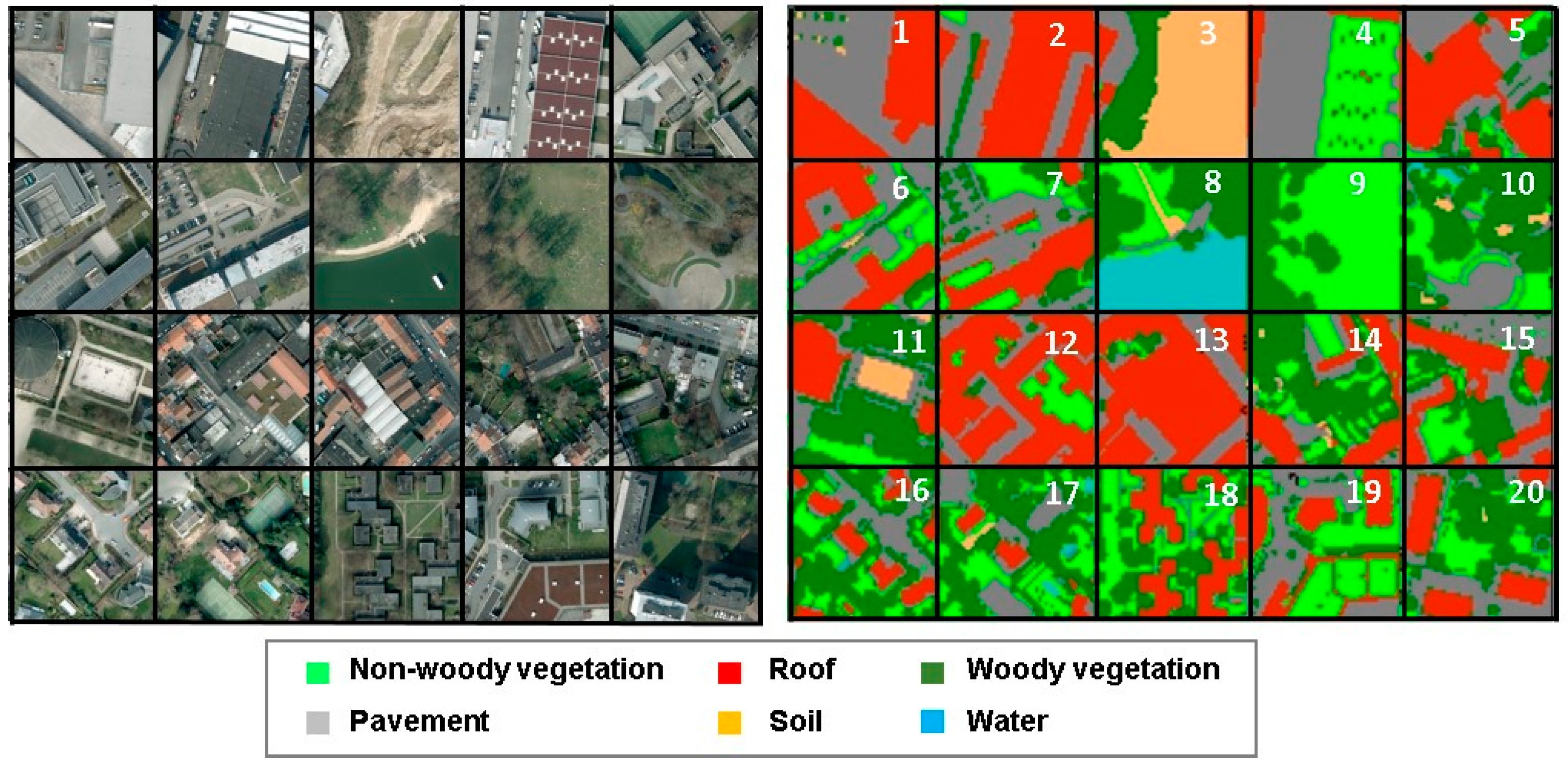
We delineated 20 blocks of 100 × 100 m (Figure 2) within our study area in which we manually digitized the urban land cover at material level. Identification of classes was done using the same ancillary data as were used during spectral library collection. The exact sample locations were selected in a stratified random way, resulting in seven industrial/commercial, four green, four dense residential and five sparse residential image blocks. The main rationale behind image block selection was to capture the urban structure types typical for the city of Brussels and to maximize the variability in image block composition. This way, we account for a representative cross-section of the city’s spectral and spatial variability, in turn allowing us to properly test the proposed pruning algorithm.
Based on these 20 validation blocks, we created 20 simulated image blocks, which were merged together into one simulated image (Figure 2). As a first step in this process, an urban material fraction map of 2 m resolution was generated based on our detailed reference data. The resulting fraction map contained 21 material classes, indicated by “x” in Table 1. Secondly, one spectrum per material class was assigned to each pixel, using a two-stage random process. A random subset of 10 spectra per material class was generated for each image block to limit the complexity within a single block and to increase the between-block variability. These subsets per image block were then randomly sampled for each pixel. In a third step, the simulated spectra were created by applying a simple linear combination of the selected spectra and the material fractions on a per-pixel basis. As a final step, we added a limited amount of Gaussian noise to the images, yielding a signal-to-noise ratio of 70 [44].

2.3.3. Experimental Setup

In our first experiment, we evaluated the performance of AMUSES using the simulated hyperspectral image and the full Brussels spectral library. Since the simulated image only includes a subset of urban materials (Table 1), the initial spectral library also contains irrelevant spectra with regard to the image. This initial library was pruned using AMUSES to produce 20 libraries, one for each image block. The following parameter settings were used based on prior experience (see Figure 1 for explanation): %retain = 5, %remove = 10, tholdhigh = 0.02, tholdlow = 0.0002. In addition, IES was applied on the initial library to generate one image-independent library subset, which served as a reference representing the state-of-the-art library-based pruning approaches. Finally, the initial library was pruned using the original MUSIC-PA to illustrate the conceptual drawbacks of the method.
The different pruning algorithms were evaluated by comparing the resulting libraries to the true set of endmembers present within each of the 20 image blocks. This was done qualitatively by visual comparison and by checking whether all the necessary land cover classes were included and no redundant classes were selected in the final libraries. In addition, a simple spectral separability index (SI) was calculated between the true endmembers and pruned libraries. SI can be defined as the ratio of inter-class variability over intra-class variability and is calculated for each land cover class and each spectral band separately using the following formula [45]:
S I i =   Δ i n t e r , i Δ i n t r a , i =   | R m e a n , i , r R m e a n , i , p | 1.96   ×   ( σ i , r +   σ i , p )
In this equation Rmean,i,r and Rmean,i,p represent the average spectral reflectance, whereas σi,r and σi,p are the standard deviation of reflectance at band i for the same land cover class in the real and pruned libraries respectively. The resulting SI values were first summed over all bands and then averaged for all land cover classes to yield one value for each combination of image block and pruning method.
Finally, the libraries were used as input into the MESMA subpixel mapping algorithm. Based on the land cover fraction maps produced by MESMA, a hard classification product was generated containing the dominant land cover class per pixel [15]. These classification maps were directly compared to the validation data for each image block by calculating a confusion matrix and subsequently deriving the total classification accuracy and kappa-statistic.

2.4. Case Study 2: Real HyMap Data Berlin

The Berlin dataset comprises a HyMap reflectance image, a library with material spectra and vegetation types relevant for the study site, and reference land cover information, all delivered as part of the Berlin-Urban-Gradient dataset [46]. In order to conduct experiments on more general libraries, we employed an additional spectral library based on HyMap data acquired over Bonn, Germany.

2.4.1. Berlin Data

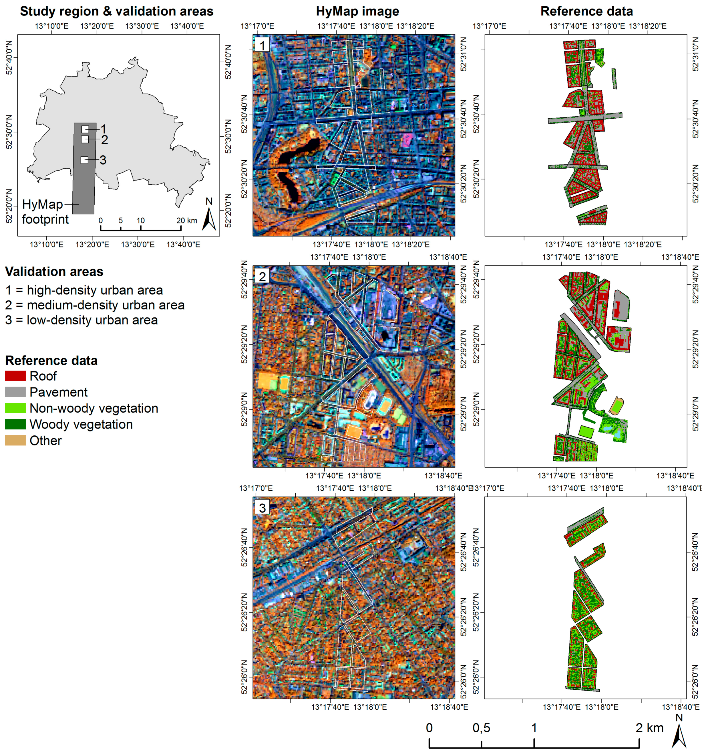
The HyMap image was acquired on 20 August 2009 at 9 m spatial resolution and covers a subset of the urban-rural gradient of Berlin, Germany (Figure 3). This way, a representative cross-section of the city’s spectral and spatial heterogeneity, ranging from a dense inner-city core to a rural urban fringe, is taken into account. The spectral library was manually extracted from a second HyMap image at 3.6 m resolution, which was acquired along the same nadir line at a similar time. For this work, the 75 original spectra were augmented by another 114 to better capture the spectral diversity and variability of materials (Table 2). The reference data represent polygon-wise land cover fractions for 55 urban blocks (ranging from 0.58 to 5.92 ha) and 17 squares of 54 × 54 m. The urban blocks represent a large range of urban land cover and structure types (e.g., building blocks, parks, streets) located within three validation areas of different urban densities. The squares cover soil-vegetation dominated plots and are located around the validation areas. Average reference fractions per block/square were calculated based on manually digitized high resolution reference land cover information. Water was not present within any of the blocks. More information on the HyMap image acquisition and pre-processing, the spectral library and reference data development are provided in [14,47].

2.4.2. Bonn Spectral Library

This spectral library was derived from 4 m resolution HyMap data acquired over the city of Bonn, Germany, in May 2005 [12]. The original library (containing 1820 spectra from individual HyMap pixels, sorted according to material class) was sampled systematically every 10th entry to yield a similarly sized library compared to the Brussels and Berlin libraries (Table 2). This specific sampling strategy was selected to make sure each material class was included in a representative way in the final subset (i.e., less spectra for less abundant classes).

2.4.3. Experimental Setup

Whereas the experiment from the previous section was designed to prove the concept of the AMUSES algorithm, the experiments conducted on the Berlin dataset focused on the added value of this pruning technique for dealing with more general spectral libraries. Subpixel fraction mapping was performed multiple times for each of our 72 validation blocks, each time starting from a different initial library that is more general compared to the previous one. Several combinations of the Berlin, Bonn and Brussels spectral libraries were generated (Table 3). In order to better match the sizes of these libraries, we created a subset of the Brussels library by sampling one every third spectrum, yielding a size of 251. The APEX spectra from Brussels (285 bands) were resampled to match the properties of the HyMap spectra (111 bands) prior to merging the two datasets.
All five initial libraries (Table 3) were pruned using both IES (yielding one library subset) and AMUSES (yielding 72 libraries, one for each image block). For both pruning techniques, the same parameter settings were used as compared to our Brussels experiment. The only exception is the %remove parameter in AMUSES, which controls the fraction of library spectra that is not considered for inclusion in the pruned library (Figure 1). This parameter was increased from 10% to 30% for all combined library experiments (experiments 2–5), as these libraries contained a higher fraction of irrelevant spectra with regard to the image. MUSIC-PA was not included in this case study, as this pruning method would require extensive re-parameterization for each of the five experiments conducted and hence is not considered as an operational pruning method.
After library pruning, ten different MESMA runs were performed for each of the 72 image blocks, i.e., one run for each combination of initial library (Table 3: ID 1 to 5) and pruning method (IES and AMUSES). The estimated land cover fractions at image block level were compared to the reference data using linear regression and associated root mean square error (RMSE). This is in line with [47,48], where a polygon-wise validation strategy was favored over pixel-wise validation due to possible geometric mismatches between the real HyMap data and the digitized validation data.

3. Results

3.1. Case Study 1: Simulated APEX Data Brussels

3.1.1. Library Pruning

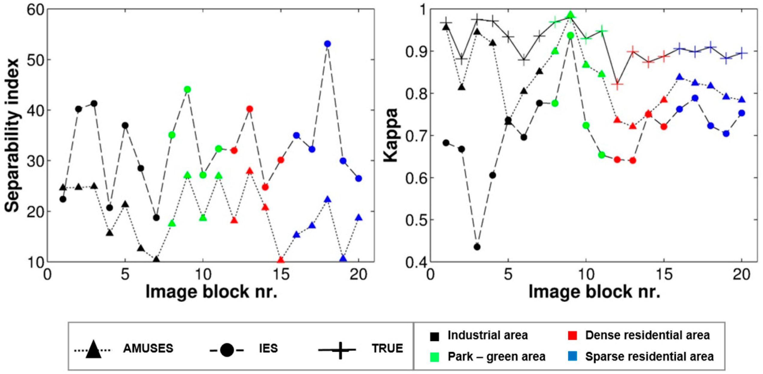
The 20 spectral libraries (one for each image block) produced using the AMUSES pruning algorithm clearly show a higher resemblance (smaller separability) to the true endmembers present within the respective image blocks compared to the IES library, the latter being the same library for all image blocks (Figure 4, left panel). IES tends to include redundant land cover classes (not occurring in a certain image block) more frequently (32 times in total) compared to AMUSES (18 times). On the other hand, both pruning techniques perfectly succeeded in selecting at least one spectrum for each land cover class present within the respective image blocks. On average, the AMUSES algorithm yields slightly larger libraries compared to IES (126 and 109 spectra respectively, compared to an average of 108 true endmembers per block).
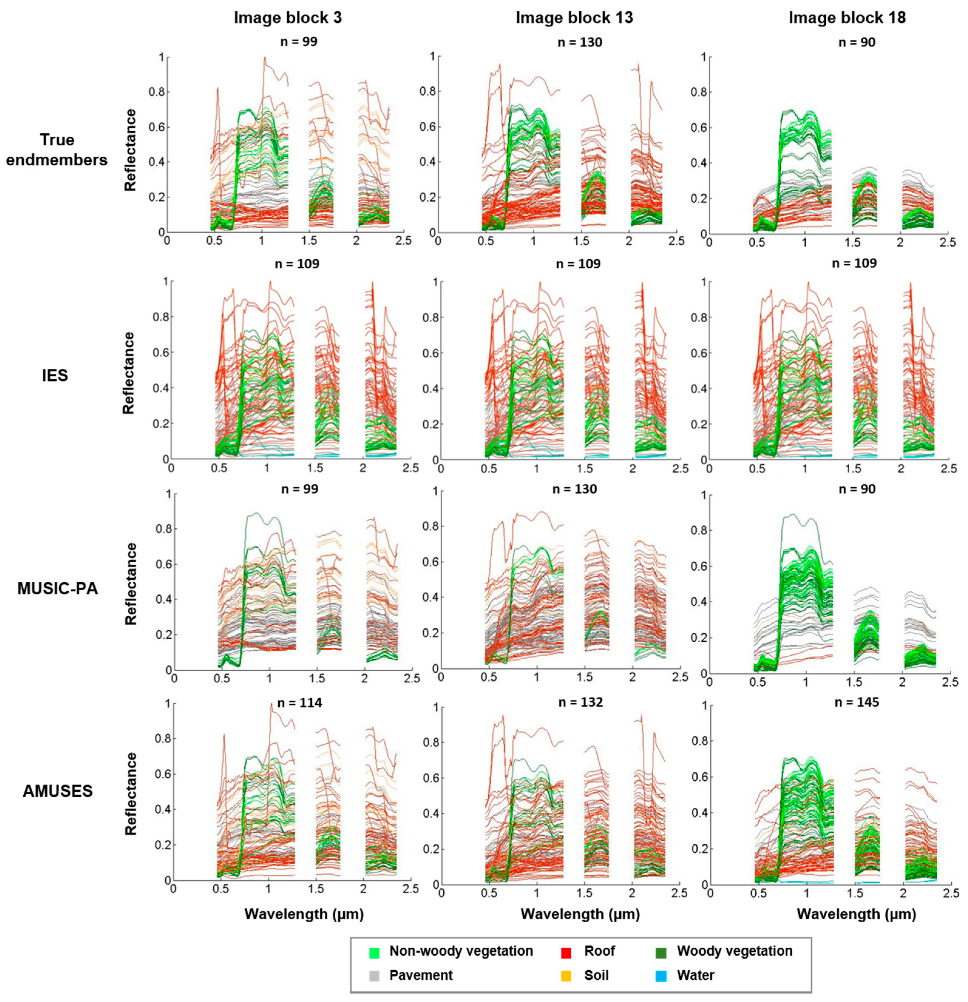
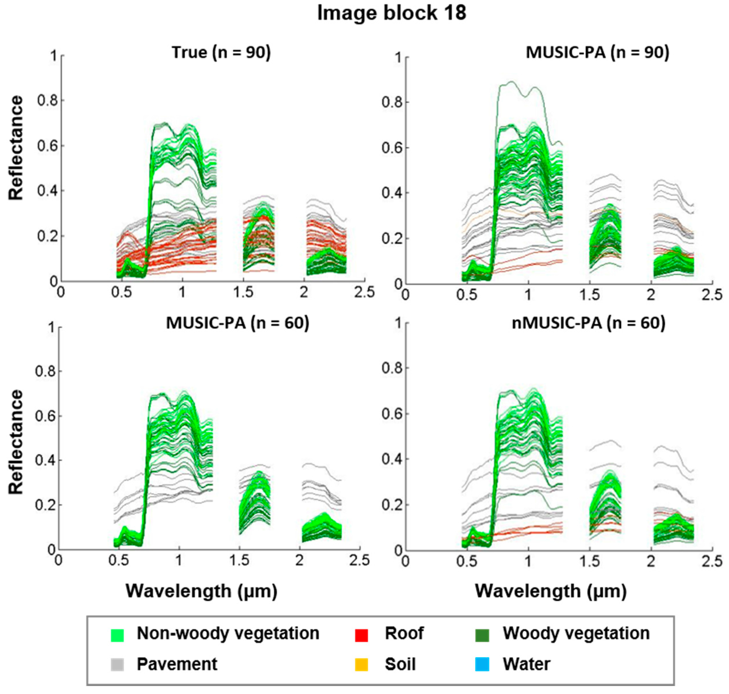
Detailed library pruning results are illustrated in Figure 5 for image blocks 3 (soil-dominated), 13 (dense residential) and 18 (sparse residential). Whereas the IES library contains a lot of irrelevant spectra (mostly roof spectra), the selection provided by AMUSES closely matches the true endmembers in the respective image blocks, visually confirming the result in the left panel of Figure 4. The original MUSIC-PA is found to produce good results, but fails to capture all variability present within the image. The drawbacks of MUSIC-PA are additionally illustrated in Figure 6 for image block 18. The comparison between the first 60 spectra selected by the original and brightness normalized versions of MUSIC-PA (two lower plots in Figure 6) shows that MUSIC-PA indeed tends to favor bright spectra and that brightness normalization causes dark spectra (in this case bitumen roof) to get selected more easily. This brightness bias can also be observed in the other two image blocks, i.e., the darkest endmembers in the images are never selected by MUSIC-PA (Figure 5). Secondly, when increasing the MUSIC-PA library size from 60 to 90 (resp. lower left and upper right plot in Figure 6), the additional spectra that get selected show a high resemblance to the ones already included and predominantly belong to the same land cover class (pavement and vegetation in this case). Likewise, MUSIC-PA selects a large collection of mutually similar pavement spectra for image block 3, but fails to include the bright and rare roof spectra present in the image (Figure 5). The automation of the AMUSES algorithm, implemented to alleviate the final drawback of MUSIC-PA (i.e., a user needs to decide on the exact number of spectra to retain), can give rise to unnecessarily large spectral libraries (as is the case for image block 18). Still, the resulting library is predominantly composed of relevant spectral signatures, particularly compared to the IES library (Figure 5).

3.1.2. Land Cover Mapping

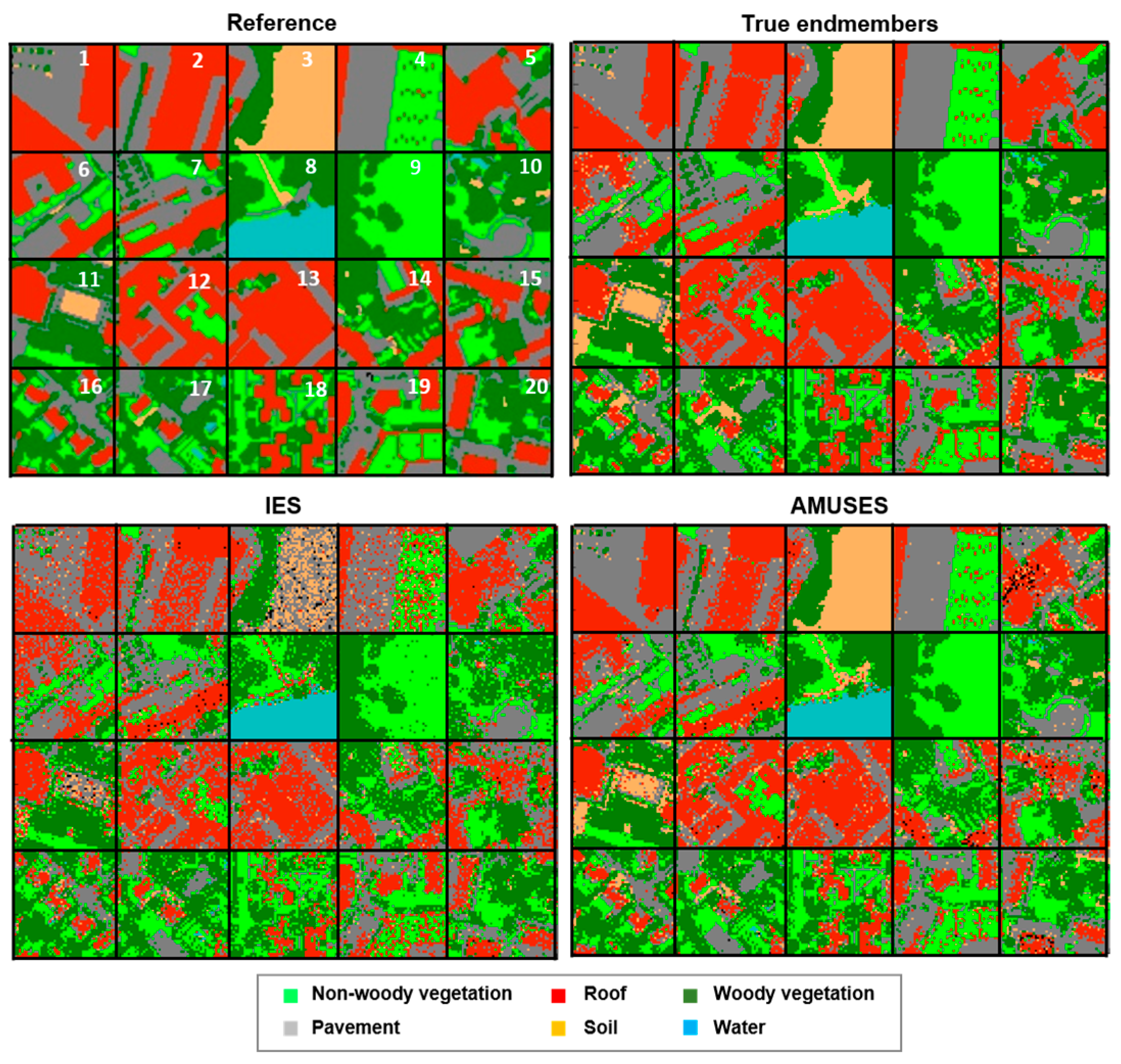
The spectral libraries obtained using AMUSES consistently yield higher mapping accuracies (expressed as kappa values) compared to the IES libraries for all image blocks (Figure 4, right panel). AMUSES most notably outperforms IES in the industrial image blocks (mainly blocks 1–4), which contain large surfaces of only a few urban materials (Figure 2). The best results are still obtained using the true set of image endmembers per block. Average kappa values/total accuracies for the true endmember set, AMUSES and IES amount to 0.92/0.95, 0.83/0.89 and 0.71/0.81 respectively. In addition, these results are visually confirmed in Figure 7, where the reference land cover map (from Figure 2) is compared to the produced land cover maps based on the true endmembers per image block, the IES library and the AMUSES libraries. The map based on the IES library clearly shows confusion between soil and pavement (e.g., image blocks 3 and 11) and between roof and pavement (e.g., image blocks 1, 2 and 4), which is much less the case for the AMUSES based result. The IES result shows a high degree of the so-called “salt-and-pepper” pattern throughout the entire map, indicating that neighboring pixels belonging to the same object on the ground are often classified differently. The AMUSES result is less affected by this effect and ground objects can be more clearly defined based on the produced map. The map generated using the true endmembers per image block shows the most resemblance to the reference map and represents the best possible outcome that can be achieved using the adopted classification approach.

3.2. Case Study 2: Real HyMap Data Berlin

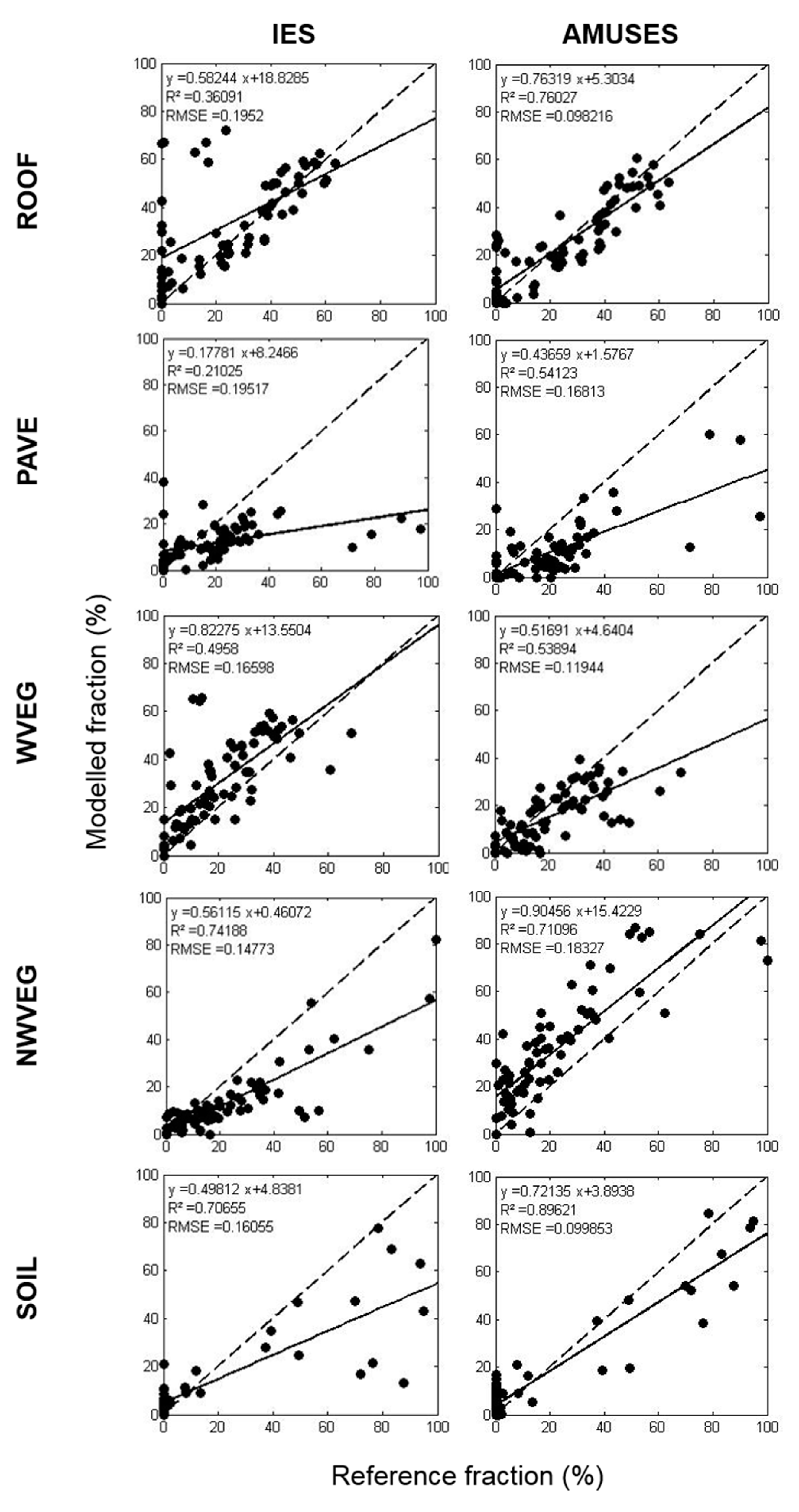
When applied to the real HyMap data of Berlin, libraries generated using AMUSES generally give rise to more accurate estimations (lower overall RMSE) of land cover fractions compared to libraries pruned using IES (Table 4). For AMUSES, highest mapping accuracies are obtained in experiments 2 and 3 (Berlin library combined with spectra from Bonn and Brussels respectively), closely followed by experiments 1 and 4 (Berlin library only and combined Berlin, Bonn and Brussels library respectively). In case of IES, the benefit of adding spectral information from other cities to the initial library is more pronounced. Here, experiment 2 (Berlin + Bonn) clearly outperforms experiment 1 (Berlin only). Both methods perform worst in case no Berlin data are available in the initial spectral library (experiment 5). The largest overall difference between AMUSES and IES is observed for experiment 1 (Berlin only). When combining the Berlin spectral library with other libraries (experiments 2–4), the net difference in mapping accuracies between AMUSES and IES decreases. The average size of the AMUSES libraries amounts to only half the size of the respective IES library and, more importantly, the former contain a significantly smaller fraction of irrelevant (i.e., non-Berlin) spectra compared to the latter (Table 4). As a result, the MESMA algorithm will more often use irrelevant spectra for modelling individual pixels if starting from the IES libraries (last column of Table 4), leading to lower overall mapping accuracies. With regard to class-wise mapping accuracies, we observe that urban materials (roof, pavement, soil) are better modelled by AMUSES. Overall, IES performs slightly better for vegetation compared to AMUSES, but this was not found to be consistent throughout the experiments, nor within one experiment for the two vegetation classes (experiment 3). The class-wise performances are illustrated for experiment 3 (Berlin-Brussels) in Figure 8. IES-based results tend to underestimate soil and pavement fractions while overestimating roof fractions. This confusion is less pronounced for AMUSES-based mapping results. Finally, in case no Berlin spectra are initially available (experiment 5), the overall performance of AMUSES libraries is slightly lower compared to IES, but the former uses on average only half the amount of spectra compared to the latter (Table 4).

4. Discussion

4.1. Library Pruning Using AMUSES

4.1.1. Performance and Advantages

Despite the large variability in image block complexity within the Brussels simulated dataset (Figure 2), AMUSES has been found to produce spectral library subsets that reasonably match the true sets of endmembers in the respective image blocks, especially compared to more traditional library pruning techniques like IES (left panel of Figure 4). After spectral unmixing, the true endmembers per image block yielded the best mapping results, closely followed by AMUSES, which in turn clearly surpassed results obtained using IES (right panel of Figure 4). This observation confirms the strong dependency of spectral unmixing results on the quality of the spectral library, ideally containing a small but relevant set of endmembers [4,49]. The same results highlight the added value of implementing AMUSES as a local pruning algorithm, producing a different, locally adapted set of endmembers for each separate image block. Even when starting from a spectral library mostly containing endmembers extracted from the image to be processed, this local approach clearly outperforms the use of one and the same library for the entire image (as done by IES). Especially in heterogeneous urban areas, typically characterized by high spectral variability [3], adopting local rather than global library pruning approaches proves to be beneficial. This is confirmed by the results from the first experiment in the Berlin case (Table 4) and by various other studies [10,12,24,25,26].
The main advantage of AMUSES compared to library based- (e.g., IES) and previously reported local pruning approaches however remains the involvement of the image within the library pruning step (i.e., the MUSIC-PA component). Whereas IES tries to ensure each land cover class in the initial spectral library is fully represented, AMUSES mostly selects library spectra that actually occur within the image block at hand. This makes the entire process much more resilient against the quality and composition of the initial spectral library. In urban areas, most spectral variability can typically be found in the roof class, being the most dominant land cover class and containing a shear variety of different materials, occurring in different stages of degradation and weathering [3,11]. The dominance of roof spectra in the initial spectral libraries (Table 1 and Table 2) causes the IES library to be predominantly composed of roof materials (Figure 5), which in turn has an impact on mapping accuracies. Recall that IES removes all spectra that can be modelled by a combination of other library entries. In the first experiment of the Berlin case study (using only Berlin spectra), all soil spectra in the initial Berlin library could be modelled by the large variety of roof endmembers, causing the resulting IES library to not include any soil spectrum. As a result, soil pixels in the image were modelled as roofs, giving rise to high errors for these two land cover classes (Table 4). AMUSES on the other hand successfully detected soil in the relevant image blocks and, due to the spectral separability component in the method, recognized it as a different material compared to the roofs present in the image. This caused the method to select at least one soil spectrum for each of these image blocks, thereby significantly improving fractional abundance estimation (Table 4). Likewise, the detailed fractional abundance results depicted in Figure 8 for the third Berlin experiment (using a combination of Berlin and Brussels spectra) show a clear overestimation of roof fractions and a resulting underestimation for soil and pavement. This bias is less pronounced for the AMUSES-based results and can again be linked to the composition of the pruned libraries. In this case, the IES library was dominated by roof spectra (53%), whereas the fraction of roof spectra in the AMUSES libraries varied between 10% and 67% (average value of 40%), depending on the composition of the specific image block.
Our experiments using simulated hyperspectral data from Brussels have shown that the original MUSIC-PA of Iordache et al. [9] in itself already performs well in selecting relevant spectra from a large collection of endmembers with regard to a certain image, even in complex and heterogeneous environments like urban areas (see Figure 5 and [31]). In this study, we further exploited this potential by combining the original algorithm with brightness normalization and a spectral separability measure. Brightness normalization successfully solved MUSIC-PA’s bias towards selecting bright spectra, which has been noted in our previous work [31] and confirmed in this study (Figure 6). As brightness typically explains an important fraction of the spectral variability in urban hyperspectral imagery [3], it will be closely correlated with the first eigenvectors extracted from the image by MUSIC-PA and will therefore greatly affect the endmember selection process. The introduction of the spectral separability measure (JMSA) alleviated MUSIC-PA’s drawback of not accounting for the similarity between the selected spectra and hence selecting redundant spectra (Figure 5). This would be particularly problematic if the initial spectral library would contain many replications of the same materials (e.g., to cover the large spectral variability of urban materials, or in a generic spectral library). In this case, the algorithm would select a group of mutually highly similar spectra, which all show a high similarity towards the few dominant materials present in the image, thereby ignoring rare image endmembers. Using MUSIC-PA, the only way to resolve this would be to retain more spectra from the original library, leading to an unnecessarily large library and thereby increasing the computation time of the subsequent unmixing procedure. The extension of MUSIC-PA with JMSA now makes it possible to easily remove redundant spectra from the final library selection. Additionally, by conceptualizing the separability threshold in AMUSES as a linear function of the similarity to the image (calculated MUSIC-PA distances, see Figure 1), the need for manually setting the number of endmembers, as required by MUSIC-PA, and the errors induced in the pruning workflow by incorrect estimation of the number of endmembers by dedicated algorithms, are avoided. It has been shown in other studies that optimizing the number of endmembers retained by MUSIC-PA for a particular combination of image and initial library can be a tedious task requiring many iterations and has a severe impact on subsequent unmixing results [31].
The automation of AMUSES does however not entail a total loss of control over the pruning procedure. In the case of IES, library pruning is fully automated and the user can only interfere by manually adding or removing endmembers after the procedure has terminated, which in practice is often required to boost its performance (e.g., [15]). In contrast, AMUSES comes with a set of clearly defined and intuitive parameters (cf. Figure 1) which can be adjusted to better match the situation at hand. However, room for improvement still remains. In this study, AMUSES’ parameter values were set for each case study based on our experience. Manually adapting the parameter values for each individual image would be highly inefficient, especially in light of the need for more universally applicable processing algorithms. Therefore, in future research more effort should be devoted to finding ways to automatically and objectively determine AMUSES’ parameters in function of both image and initial spectral library complexity. For instance, the %remove parameter, which controls the fraction of most dissimilar spectra from the original library that will not be considered during library pruning (Figure 1), is highly dependent on the quality of the initial spectral library (i.e., the fraction of irrelevant spectra with regard to the image). In our study, this has been accounted for by increasing this parameter from 10% to 30% when dealing with more general spectral libraries. Less experienced users of AMUSES are advised to first optimize the value of the %remove parameter when applying AMUSES in a new setting, as this parameter is more intuitive compared to the tholdlow and tholdhigh parameters. The latter two have been optimized using the Brussels data and have been held constant throughout the remainder of this study. Despite the large differences between the experiments in terms of image data (sensor, resolution) and initial spectral libraries, these parameter values were found to yield decent pruning results. The chosen values therefore represent a good initial estimate whenever AMUSES would be adopted in another case study.
In the Brussels experiment, AMUSES was found to produce spectral libraries much larger than the true set of endmembers, particularly for low complexity image blocks (e.g., block 18 in Figure 5). By decreasing the number of eigenvectors to be retained by the MUSIC-PA (nEigenv) from the default value of 15 (Figure 1) to only 5, AMUSES produced a significantly smaller set of endmembers containing less irrelevant spectra for this image block (86 vs. 145 spectra; compared to 90 true endmembers). Decreasing nEigenv leads to an increase in the variability of the calculated MUSIC-PA distances. Due to the linear relation between the spectral separability threshold (thold parameter) and the normalized MUSIC-PA distances (Figure 1), this change will impact the endmember selection procedure, which will be more strict, causing a decrease in final library size. Ideally, the nEigenv parameter should hence be defined in function of image complexity, e.g., using a semivariogram approach [10].

4.1.2. Potential for Processing Generic Spectral Libraries

Our additional experiments combining multiple libraries from different origins into more general libraries to unmix HyMap imagery from Berlin have clearly shown the potential of AMUSES to successfully deal with generic spectral libraries. Whereas IES once again tries to account for all the variability present within the initial libraries and selects a substantial amount of irrelevant spectra (in this case non-Berlin spectra), AMUSES is clearly able to select the relevant spectra from a mixed library (next to last column in Table 4). As a result, MESMA will more often use irrelevant spectra for modelling image pixels if starting from the IES library (last column in Table 4), immediately explaining the lower overall mapping accuracies observed for IES compared to AMUSES. In general, Table 4 indicates that AMUSES produces better unmixing results using less (but more relevant) spectral information and hence requires less computational efforts. The only exception is experiment 5, in which no Berlin spectra are available and AMUSES performs slightly worse compared to IES. In this case, AMUSES produced a library subset that is too small to capture all endmember variability within the Berlin image (i.e., less than half the size of the IES library; Table 4). This is confirmed by the number of unmodelled pixels contained in the MESMA hard classification product: 283 pixels for AMUSES versus only 41 pixels for IES (not shown). Whenever the original spectral library contains no information from the image to be processed, more spectra will be needed to fully capture the true endmember variability within that image. When we decreased the %remove parameter in AMUSES from 30% to 10%, the average number of spectra in the resulting libraries increased to 51, in turn yielding a lower RMSE (0.21, same as for IES) and a lower amount of unmodelled pixels (165), which confirms our hypothesis. Looking in closer detail, the IES library for this experiment is dominated by Brussels spectra (75%), whereas the different AMUSES libraries on average only contain 21% of Brussels spectra. Given the origin (i.e., sensor and location) of the Bonn and Brussels spectral libraries, the former can be objectively considered as the most relevant for unmixing the Berlin imagery, implying that, from a library pruning perspective, AMUSES still outperformed IES.
In our Berlin case study, we have shown the potential of AMUSES for dealing with spectral libraries derived from various sources, thereby paving the way for the widespread adoption and integration of generic spectral libraries in spectral unmixing workflows of urban (and other) areas. This development is supported by another trend in remote sensing, i.e., the gathering of spectral information from all possible sources into huge online libraries (e.g., USGS spectral library [50], SPECCHIO database [51]). As new methods are arising to automatically complete these libraries by cross-checking them with pure spectral information contained in imagery (e.g., LUISA [52]), the availability of endmembers for unmixing purposes is expected to rise exponentially. The only way to process such huge sets of endmember libraries is through the use of smart pruning algorithms, capable of handling such generic databases. The libraries used in our experiments are still relatively small and derived from a small set of images largely containing similar urban materials (all Western European cities). Future research should therefore further explore the potential of AMUSES to deal with larger, even more generic libraries. Likewise, although our experiments already incorporated multi-resolution data (2, 3.6, 4 and 9 m), additional tests on low resolution satellite imagery (30 m) will need to be conducted to fully establish our method’s ability for dealing with imagery containing increasing degrees of spectral mixtures. The latter would be particularly relevant in light of upcoming hyperspectral satellite missions [1,2].
By comparing experiments 2 and 3 from our Berlin case study (i.e., using Berlin in combination with Bonn or Brussels spectral libraries), we noticed AMUSES tends to select more Bonn spectra compared to Brussels spectra for unmixing Berlin imagery. This phenomenon can be either caused by regional differences in urban material composition or by sensor-specific differences (HyMap vs. APEX). Especially differences in pre-processing of the image data (reflectance retrieval) can have a significant impact on the quality of the image spectra, which complicates studies that aim at transferring training information to other sites (e.g., [53]). Particularly in light of the adoption of generic spectral libraries, harmonization of multi-source spectral libraries and image data requires further attention by the remote sensing community.

4.1.3. Additional Applications

In this study, AMUSES has been applied as a local library pruning tool on individual image blocks of constant (Brussels) or varying (Berlin) sizes for which detailed validation data were available. For mapping an entire image, this would be translated into a moving window approach, in which the image would be partitioned into multiple areas of equal size, each for which one set of locally relevant endmembers would be produced. Based on our experiment in Brussels, we conclude that the efficiency of AMUSES compared to conventional pruning techniques is largest for image subsets containing few endmembers. This implies that, in an operational setting, the size of the moving window (controlling complexity of the image subsets) would be a crucial parameter determining the success of AMUSES. Ideally, this parameter should be determined in an objective way, based on the complexity of the entire image (cf. semivariogram approach used by [10]). An alternative approach would be to first conduct an object-based classification of the image, producing image segments of comparable complexity, as was done by [10,26]. The latter approach would potentially circumvent the need to redefine the parameter set of the AMUSES algorithm for each image subset.
Here we successfully combined AMUSES with MESMA to produce accurate subpixel abundance fractions of different urban areas. As our pruning algorithm operates independently from the actual unmixing step, AMUSES can theoretically be combined with any other spectral unmixing algorithm that makes use of spectral libraries to cope with endmember variability. In particular, the combination with sparse unmixing would be an interesting approach to explore, given the fact that MUSIC-PA has been specifically developed in combination with a collaborative sparse regression technique [54]. Moreover, AMUSES could prove useful in combination with machine learning-based approaches. Okujeni et al. [47] for instance developed a method that trains a set of support vector regression models for mapping urban land cover using a large set of synthetically mixed training data generated from a spectral library. A smart, a-priori selection of synthetically mixed endmembers that are relevant to the image at hand could potentially increase the computational efficiency of this algorithm.

4.2. Urban Land Cover Mapping Using Hyperspectral Imagery

In general, the accuracy values of our spectral unmixing results, obtained using a combination of AMUSES and MESMA, are in line with typical values found by other studies in the urban environment, using a variety of different image data, library pruning approaches and spectral unmixing techniques [16,47,55,56,57]. In particular, overall RMSE values from our first experiment on the Berlin data closely match the performance reported by a study conducted on the same data using machine learning-based approaches [48]. However, significant mapping errors were still observed, particularly the overestimation of roof and underestimation of pavement and soil (Figure 8). The same problems are observed by other urban mapping studies (e.g., [16,48]) and are caused by the well-known phenomenon of spectral confusion between soil, pavement and roof materials, which are typically made of the same materials (e.g., asphalt roads and bitumen roofs [3,11]). In response to these limitations, many studies have already suggested and successfully proven the added benefits of fusing hyperspectral data with various other data, especially LiDAR data, for urban land cover mapping (e.g., [16,56,57,58]). Although AMUSES has shown clear potential towards the development of universal mapping workflows for urban areas, we acknowledge that one algorithm is not likely to solve all problems related to urban mapping and therefore plead for an optimal integration of different techniques based on various data sources.

5. Conclusions

The vast amount of (hyper) spectral data currently being collected over urban areas around the globe presents interesting opportunities for detailed characterization and monitoring of urban land cover, but at the same time requires highly efficient and transferable processing algorithms. Using generic spectral libraries, e.g., by merging existing urban spectral libraries from various sources, as training data for spectral unmixing represents a viable alternative to the tedious task of collecting endmembers for each individual image. Given the size of such a generic database, the workflow would require an efficient spectral library pruning technique, which allows to select from this generic database the smallest, most relevant set of endmembers required to produce accurate mapping results for each image. In this context, we proposed the AMUSES algorithm, which effectively combines the strengths of three different library pruning concepts. Using both simulated and real hyperspectral datasets from two different cities, sensors and resolutions, we proved AMUSES successfully manages to select relevant endmembers from a relatively large spectral database, thereby significantly increasing the mapping accuracies obtained using Multiple Endmember Spectral Mixture Analysis (MESMA) compared to more traditional pruning approaches. Although further improvement of the proposed AMUSES algorithm is still possible, especially in terms of finding objective ways to define its parameters in function of image and initial library complexity, the experiments in this study clearly illustrated its potential for dealing with generic spectral databases. Further tests including a wider variety of spectral libraries and low resolution hyperspectral imagery are still desirable before the widespread adoption and integration of AMUSES in universal workflows for mapping urban land cover.

Acknowledgments

The research presented in this paper is funded by the Belgian Science Policy Office in the framework of the STEREOIII program (projects UrbanEARS (SR/00/307) and VIPER2 (SR/XX/171)). The authors would like to acknowledge Frederik Priem, Marie-Leen Verdonck and Charlotte Wirion for their help in gathering land cover validation data in the Brussels region. Special thanks also goes to Frederik Priem for providing an extensive spectral library of the Brussels urban region. Finally, the authors are grateful to Dar Roberts for the critical evaluation of this work and for providing the Bonn spectral library.

Author Contributions

Jeroen Degerickx created the library pruning method presented in this paper, designed, performed and interpreted the experiments and wrote the main part of the manuscript. All co-authors actively contributed to the manuscript writing and approved the final version of the manuscript. Additionally, Akpona Okujeni aided in designing and interpreting the experiments. The expertise of Marian-Daniel Iordache regarding the MUSIC pruning algorithm was actively used for designing the AMUSES algorithm. Martin Hermy contributed mainly to the discussion of the broader applicability of our methodology and overall implications of this work. Ben Somers, the main supervisor of this research, together with Sebastian van der Linden conceived the central concepts of the generic library approach presented here and additionally aided in designing and interpreting the experiments.

Conflicts of Interest

The authors declare no conflict of interest.

References

  1. Guanter, L.; Kaufmann, H.; Segl, K.; Foerster, S.; Rogass, C.; Chabrillat, S.; Kuester, T.; Hollstein, A.; Rossner, G.; Chlebek, C.; et al. The EnMAP Spaceborne Imaging Spectroscopy Mission for Earth Observation. Remote Sens. 2015, 7, 8830–8857. [Google Scholar] [CrossRef]
  2. Lee, C.M.; Cable, M.L.; Hook, S.J.; Green, R.O.; Ustin, S.L.; Mandl, D.J.; Middleton, E.M. An introduction to the NASA Hyperspectral InfraRed Imager (HyspIRI) mission and preparatory activities. Remote Sens. Environ. 2015, 167, 6–19. [Google Scholar] [CrossRef]
  3. Herold, M.; Gardner, M.E.; Roberts, D.A. Spectral resolution requirements for mapping urban areas. IEEE Trans. Geosci. Remote Sens. 2003, 41, 1907–1919. [Google Scholar] [CrossRef]
  4. Roberts, D.A.; Gardner, M.; Church, R.; Ustin, S.; Scheer, G.; Green, R.O. Mapping chaparral in the Santa Monica Mountains using multiple endmember spectral mixture models. Remote Sens. Environ. 1998, 65, 267–279. [Google Scholar] [CrossRef]
  5. Asner, G.P.; Lobell, D.B. A biogeophysical approach for automated SWIR unmixing of soils and vegetation. Remote Sens. Environ. 2000, 74, 99–112. [Google Scholar] [CrossRef]
  6. Song, C. Spectral mixture analysis for subpixel vegetation fractions in the urban environment: How to incorporate endmember variability? Remote Sens. Environ. 2005, 95, 248–263. [Google Scholar] [CrossRef]
  7. Iordache, M.-D.; Bioucas-Dias, J.M.; Plaza, A. Sparse Unmixing of Hyperspectral Data. IEEE Trans. Geosci. Remote Sens. 2011, 49, 2014–2039. [Google Scholar] [CrossRef]
  8. Somers, B.; Tits, L.; Roberts, D.A.; Wetherley, E.B. Endmember library approaches to resolve spectral mixing problems in remotely sensed data: Potential, challenges, and applications. In Data Handling in Science and Technology; Elsevier: Amsterdam, The Netherlands, 2016. [Google Scholar]
  9. Iordache, M.D.; Bioucas-Dias, J.M.; Plaza, A.; Somers, B. MUSIC-CSR: Hyperspectral unmixing via multiple signal classification and collaborative sparse regression. IEEE Trans. Geosci. Remote Sens. 2014, 52, 4364–4382. [Google Scholar] [CrossRef]
  10. Deng, C. Automated Construction of Multiple Regional Libraries for Neighborhoodwise Local Multiple Endmember Unmixing. IEEE J. Sel. Top. Appl. Earth Obs. Remote Sens. 2016, 9, 4232–4246. [Google Scholar] [CrossRef]
  11. Heiden, U.; Segl, K.; Roessner, S.; Kaufmann, H. Determination of robust spectral features for identification of urban surface materials in hyperspectral remote sensing data. Remote Sens. Environ. 2007, 111, 537–552. [Google Scholar] [CrossRef]
  12. Franke, J.; Roberts, D.A.; Halligan, K.; Menz, G. Hierarchical Multiple Endmember Spectral Mixture Analysis (MESMA) of hyperspectral imagery for urban environments. Remote Sens. Environ. 2009, 113, 1712–1723. [Google Scholar] [CrossRef]
  13. Kotthaus, S.; Smith, T.E.L.; Wooster, M.J.; Grimmond, C.S.B. Derivation of an urban materials spectral library through emittance and reflectance spectroscopy. ISPRS J. Photogramm. Remote Sens. 2014, 94, 194–212. [Google Scholar] [CrossRef]
  14. Okujeni, A.; van der Linden, S.; Hostert, P. Extending the vegetation-impervious-soil model using simulated EnMAP data and machine learning. Remote Sens. Environ. 2015, 158, 69–80. [Google Scholar] [CrossRef]
  15. Roberts, D.; Alonzo, M.; Wetherley, E.B.; Dudley, K.L.; Dennison, P.E. Multiscale Analysis of Urban Areas Using Mixing Models. In Integrating Scale in Remote Sensing and GIS; CRC Press: New York, NY, USA, 2016; pp. 247–282. [Google Scholar]
  16. Priem, F.; Canters, F. Synergistic Use of LiDAR and APEX Hyperspectral Data for High-Resolution Urban Land Cover Mapping. Remote Sens. 2016, 8, 787. [Google Scholar] [CrossRef]
  17. Wetherley, E.B.; Roberts, D.A.; McFadden, J. Mapping spectrally similar urban materials at sub-pixel scales. Remote Sens. Environ. 2017, 195, 170–183. [Google Scholar] [CrossRef]
  18. Dudley, K.L.; Dennison, P.E.; Roth, K.L.; Roberts, D.A.; Coates, A.R. A multi-temporal spectral library approach for mapping vegetation species across spatial and temporal phenological gradients. Remote Sens. Environ. 2015, 167, 121–134. [Google Scholar] [CrossRef]
  19. Dennison, E.P.; Roberts, A.D. Endmenber selection for multiple endmenber spectral mixture analysis using endmember average RMSE. Remote Sens. Environ. 2003, 87, 123–135. [Google Scholar] [CrossRef]
  20. Roberts, D.A.; Dennison, P.E.; Gardner, M.E.; Hetzel, Y.; Ustin, S.L.; Lee, C.T. Evaluation of the potential of hyperion for fire danger assessment by comparison to the airborne visible/infrared imaging spectrometer. IEEE Trans. Geosci. Remote Sens. 2003, 41, 1297–1310. [Google Scholar] [CrossRef]
  21. Dennison, P.E.; Halligan, K.Q.; Roberts, D.A. A comparison of error metrics and constraints for multiple endmember spectral mixture analysis and spectral angle mapper. Remote Sens. Environ. 2004, 93, 359–367. [Google Scholar] [CrossRef]
  22. Schaaf, A.N.; Dennison, P.E.; Fryer, G.K.; Roth, K.L.; Roberts, D.A. Mapping plant functional types at multiple spatial resolutions using imaging spectrometer data. GIScience Remote Sens. 2011, 48, 324–344. [Google Scholar] [CrossRef]
  23. García-Haro, F.J.; Sommer, S.; Kemper, T. A new tool for variable multiple endmember spectral mixture analysis (VMESMA). Int. J. Remote Sens. 2005, 26, 2135–2162. [Google Scholar] [CrossRef]
  24. Liu, T.; Yang, X. Mapping vegetation in an urban area with stratified classification and multiple endmember spectral mixture analysis. Remote Sens. Environ. 2013, 133, 251–264. [Google Scholar] [CrossRef]
  25. Deng, Y.; Wu, C. Development of a Class-Based Multiple Endmember Spectral Mixture Analysis (C-MESMA) Approach for Analyzing Urban Environments. Remote Sens. 2016, 8, 349. [Google Scholar] [CrossRef]
  26. Zhang, C.; Cooper, H.; Selch, D.; Meng, X.; Qiu, F.; Myint, S.W.; Roberts, C.; Xie, Z. Mapping urban land cover types using object-based multiple endmember spectral mixture analysis. Remote Sens. Lett. 2014, 5, 521–529. [Google Scholar] [CrossRef]
  27. Fan, F.; Deng, Y. Enhancing endmember selection in multiple endmember spectral mixture analysis (MESMA) for urban impervious surface area mapping using spectral angle and spectral distance parameters. Int. J. Appl. Earth Obs. Geoinf. 2014, 33, 290–301. [Google Scholar] [CrossRef]
  28. Chen, F.; Wang, K.; Tang, T.F. Spectral Unmixing Using a Sparse Multiple-Endmember Spectral Mixture Model. IEEE Trans. Geosci. Remote Sens. 2016, 54, 5846–5861. [Google Scholar] [CrossRef]
  29. Bienvenu, G.; Kopp, L. Adaptivity to background noise spatial coherence for high resolution passive methods. In Proceedings of the IEEE International Conference on Acoustics, Speech, and Signal, Denver, CO, USA, 9–11 April 1980. [Google Scholar]
  30. Schmidt, R. Multiple emitter location and signal parameter estimation. IEEE Trans. Antennas Propag. 1986, 34, 276–280. [Google Scholar] [CrossRef]
  31. Degerickx, J.; Iordache, M.-D.; Okujeni, A.; Hermy, M.; van der Linden, S.; Somers, B. Spectral unmixing of urban land cover using a generic library approach. In Proceedings of the SPIE 10008, Remote Sensing Technologies and Applications in Urban Environments, Edinburgh, UK, 26 September 2016. [Google Scholar]
  32. Pauleit, S.; Duhme, F. Assessing the environmental performance of land cover types for urban planning. Landsc. Urban Plan. 2000, 52, 1–20. [Google Scholar] [CrossRef]
  33. Cadenasso, M.L.; Pickett, S.T.A.; Schwarz, K. Spatial heterogeneity in urban ecosystems: Conceptualizing land cover and a framework for classification. Front. Ecol. Environ. 2007, 5, 80–88. [Google Scholar] [CrossRef]
  34. Bioucas-Dias, J.M.; Nascimento, J.M.P. Hyperspectral Subspace Identification. IEEE Trans. Geosci. Remote Sens. 2008, 46, 2435–2445. [Google Scholar] [CrossRef]
  35. Wu, C. Normalized spectral mixture analysis for monitoring urban composition using ETM+ imagery. Remote Sens. Environ. 2004, 93, 480–492. [Google Scholar] [CrossRef]
  36. Padma, S.; Sanjeevi, S. Jeffries Matusita based mixed-measure for improved spectral matching in hyperspectral image analysis. Int. J. Appl. Earth Obs. Geoinf. 2014, 32, 138–151. [Google Scholar] [CrossRef]
  37. Adams, J.B.; Smith, M.O.; Johnson, P.E. Spectral mixture modeling: A new analysis of rock and soil types at the Viking Lander 1 Site. J. Geophys. Res. Solid Earth 1986, 91, 8098–8112. [Google Scholar] [CrossRef]
  38. Powell, R.L.; Roberts, D.A. Characterizing variability of the urban physical environment for a suite of cities in Rondônia, Brazil. Earth Interact. 2008, 12, 1–32. [Google Scholar] [CrossRef]
  39. Demarchi, L.; Canters, F.; Chan, J.C.W.; Van De Voorde, T. Multiple endmember unmixing of CHRIS/proba imagery for mapping impervious surfaces in urban and suburban environments. IEEE Trans. Geosci. Remote Sens. 2012, 50, 3409–3424. [Google Scholar] [CrossRef]
  40. Biesemans, J.; Sterckx, S.; Knaeps, E.; Vreys, K.; Adriaensen, S.; Hooy-, J. Image Processing Workflows for Airborne Remote. In Proceedings of the 5th EARSeL Workshop on Imaging Spectroscopy, Bruges, Belgium, 23–25 April 2007; pp. 1–14. [Google Scholar]
  41. Vreys, K.; Iordache, M.D.; Biesemans, J.; Meuleman, K. Geometric correction of APEX hyperspectral data. Misc. Geogr. 2016, 20, 11–15. [Google Scholar] [CrossRef]
  42. Berk, A.; Anderson, G.P.; Bernstein, L.S.; Acharya, P.K.; Dothe, H.; Matthew, M.W.; Adler-Golden, S.M.; Chetwynd, J.H., Jr.; Richtsmeier, S.C.; Pukall, B.; et al. MODTRAN4 radiative transfer modeling for atmospheric correction. Pcoceedings of the Optical Spectroscopic Techniques and Instrumentation for Atmospheric and Space Research III, Denver, CO, USA, 18 July 1999. [Google Scholar]
  43. Sterckx, S.; Vreys, K.; Biesemans, J.; Iordache, M.-D.; Bertels, L.; Meuleman, K. Atmospheric correction of APEX hyperspectral data. Misc. Geogr. 2016, 20, 16–20. [Google Scholar] [CrossRef]
  44. Somers, B.; Delalieux, S.; Verstraeten, W.W.; Verbesselt, J.; Lhermitte, S.; Coppin, P. Magnitude- and Shape-Related Feature Integration in Hyperspectral Mixture Analysis to Monitor Weeds in Citrus Orchards. IEEE Trans. Geosci. Remote Sens. 2009, 47, 3630–3642. [Google Scholar] [CrossRef]
  45. Somers, B.; Asner, G.P. Tree species mapping in tropical forests using multi-temporal imaging spectroscopy: Wavelength adaptive spectral mixture analysis. Int. J. Appl. Earth Obs. Geoinf. 2014, 31, 57–66. [Google Scholar] [CrossRef]
  46. Okujeni, A.; van der Linden, S.; Hostert, P. Berlin-Urban-Gradient Dataset 2009—An EnMAP Preparatory Flight Campaign (Datasets). Available online: http://dataservices.gfz-potsdam.de/enmap/showshort.php?id=escidoc:1823890 (accessed on 27 March 2017).
  47. Okujeni, A.; van der Linden, S.; Tits, L.; Somers, B.; Hostert, P. Support vector regression and synthetically mixed training data for quantifying urban land cover. Remote Sens. Environ. 2013, 137, 184–197. [Google Scholar] [CrossRef]
  48. Okujeni, A.; van der Linden, S.; Jakimow, B.; Rabe, A.; Verrelst, J.; Hostert, P. A comparison of advanced regression algorithms for quantifying urban land cover. Remote Sens. 2014, 6, 6324–6346. [Google Scholar] [CrossRef]
  49. Tompkins, S.; Mustard, J.F.; Pieters, C.M.; Forsyth, D.W. Optimization of endmembers for spectral mixture analysis. Remote Sens. Environ. 1997, 59, 472–489. [Google Scholar] [CrossRef]
  50. USGS Digital Spectral Library 06. Available online: http://purl.access.gpo.gov/GPO/LPS89885 (accessed on 26 March 2017).
  51. Hueni, A.; Nieke, J.; Schopfer, J.; Kneubühler, M.; Itten, K.I. The spectral database SPECCHIO for improved long-term usability and data sharing. Comput. Geosci. 2009, 35, 557–565. [Google Scholar] [CrossRef]
  52. Jilge, M.; Heiden, U.; Habermeyer, M.; Mende, A.; Juergens, C.; Glauchau, D. Identifying pure urban image spectra using a learning urban image spectral archive (LUISA). In Proceedings of the SPIE 10008, Remote Sensing Technologies and Applications in Urban Environments, Edinburgh, UK, 26 September 2016. [Google Scholar]
  53. Tuia, D.; Marcos, D.; Camps-Valls, G. Multi-temporal and multi-source remote sensing image classification by nonlinear relative normalization. ISPRS J. Photogramm. Remote Sens. 2016, 120, 1–12. [Google Scholar] [CrossRef]
  54. Iordache, M.-D.; Bioucas-Dias, J.M.; Plaza, A. Collaborative Sparse Regression for Hyperspectral Unmixing. IEEE Trans. Geosci. Remote Sens. 2014, 52, 341–354. [Google Scholar] [CrossRef]
  55. Herold, M.; Scepan, J.; Günther, S.; Müller, A. Object-oriented mapping and analysis of urban land use/cover using IKONOS data. In Proceedings of the 22nd Earsel Symposium Geoinformation for European-Wide Integration, Prague, Czech Republic, 4–7 June 2002. [Google Scholar]
  56. Tong, X.; Xie, H.; Weng, Q. Urban Land Cover Classification with Airborne Hyperspectral Data: What Features to Use? IEEE J. Sel. Top. Appl. Earth Obs. Remote Sens. 2014, 7, 3998–4009. [Google Scholar] [CrossRef]
  57. Akbari, D.; Homayouni, S.; Safari, A.; Mehrshad, N. Mapping urban land cover based on spatial-spectral classification of hyperspectral remote-sensing data. Int. J. Remote Sens. 2016, 37, 440–454. [Google Scholar] [CrossRef]
  58. Heiden, U.; Heldens, W.; Roessner, S.; Segl, K.; Esch, T.; Mueller, A. Urban structure type characterization using hyperspectral remote sensing and height information. Landsc. Urban Plan. 2012, 105, 361–375. [Google Scholar] [CrossRef]
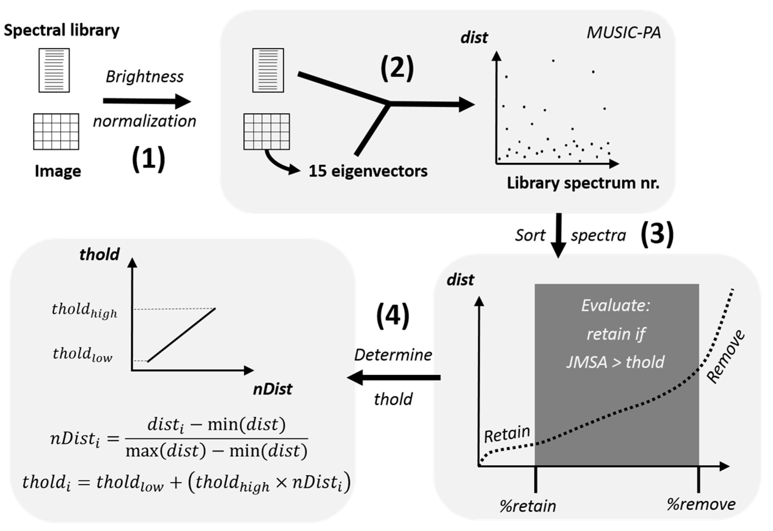
Figure 1. Workflow of the AMUSES pruning algorithm. (1) Brightness normalization is applied on the original image and spectral library to avoid the brightness bias of the original MUSIC-PA. (2) MUSIC-PA: the image is represented as 15 eigenvectors and the distance (dist) of each library spectrum to this set of eigenvectors is determined. (3) Spectra are sorted according to their MUSIC-PA distance. A fraction of the most relevant spectra (%retain) is retained, a fraction of the least relevant (%remove) is discarded. The other spectra are evaluated using the JMSA spectral separability metric (combining Jeffries Matusita distance and Spectral Angle): a spectrum is only retained if it is sufficiently dissimilar (JMSA larger than a threshold, thold) from the already selected spectra. (4) The JMSA threshold is determined in function of the normalized MUSIC-PA distance (nDist) for each spectrum: the higher the distance, the less relevant the spectrum is to the image under consideration and the more dissimilar it needs to be from the already selected spectra in order to get selected.
Remotesensing 09 00565 g001
Figure 2. Orthophoto (left) and digitized validation data (right) of the twenty 100 × 100 m blocks used to create the simulated dataset of Brussels. The image blocks can be categorized into four distinct urban structure types: industrial/commercial (blocks 1–7), green areas/parks (blocks 8–11), dense residential (blocks 12–15) and sparse residential (blocks 16–20).
Remotesensing 09 00565 g002
Figure 3. Berlin study area, along with the HyMap image (R = 833 nm, G = 1652 nm, B = 632 nm) and high resolution reference data for the three validation areas (polygons indicate the urban blocks used for validation).
Remotesensing 09 00565 g003
Figure 4. Performance comparison of IES and AMUSES pruning algorithms on the 20 image blocks of the Brussels dataset. Left: Spectral separability between pruned and true endmember libraries. Right: MESMA mapping accuracies (presented by kappa value) based on the respective libraries compared to using the true set of endmembers present in the image blocks (TRUE). Data points are color coded in function of the urban structure type of the image blocks.
Remotesensing 09 00565 g004
Figure 5. Comparison of true endmembers versus pruned libraries generated using IES, the original MUSIC-PA and the proposed AMUSES algorithm for image blocks 3, 13 and 18 (cf. Figure 2). The symbol “n” represents the size of the spectral library. The number of spectra to be retained by MUSIC-PA was manually set to match the true number of endmembers in the respective image blocks.
Remotesensing 09 00565 g005
Figure 6. In case of image block 18, the original MUSIC-PA mainly selects vegetation spectra (upper right panel), whereas the image itself is mainly dominated by roof (illustrated by the true endmembers in the upper left panel). When decreasing the number of spectra in the final library size to 60 (lower left panel), no roof is selected at all, which would have severe implications on the subsequent mapping of this image. This panel also shows the brightness bias of MUSIC-PA, mainly selecting bright spectra. By applying brightness normalization (nMUSIC-PA, lower right panel), this bias is clearly reduced.
Remotesensing 09 00565 g006
Figure 7. Reference land cover map compared to the different land cover maps produced for the Brussels case study by applying MESMA on different spectral libraries, i.e., the true endmembers present in the image blocks, a library obtained using Iterative Endmember Selection (IES) and one obtained using the newly proposed AMUMSES algorithm. The classification product developed using the true endmembers slightly deviates from the reference data due to the noise introduced in the simulated image and minor modelling errors in the MESMA-based classification procedure.
Remotesensing 09 00565 g007
Figure 8. Comparison of reference (x-axis) versus modelled (y-axis) land cover fractions for 72 image blocks of the Berlin dataset. Modelled results are obtained by applying MESMA on a spectral library pruned using IES (left) and AMUSES (right). The original spectral library consisted of a mixture of Berlin and Brussels spectral libraries (experiment 3 in Table 3). PAVE = pavement; WVEG = woody vegetation; NWVEG = non-woody vegetation.
Remotesensing 09 00565 g008
Table 1. Brussels spectral library organized per land cover class, including an indication of library size per urban material or vegetation type and whether or not the material or type has been used in the creation of the simulated image (all included materials are indicated using the symbol “x”).
Land Cover ClassesMaterial/TypeNumber of SpectraSimulation
RoofBitumen26x
Bright roof material22x
Dark ceramic tile31x
Dark shingle29
Fiber cement24
Glass11x
Gray metal26x
Gravel roofing25x
Green metal16x
Hydrocarbon roofing24
Paved terrace12
Red ceramic tile33x
Solar panel25
PavementArtificial turf22
Asphalt 24x
Bright gravel15
Cobblestone16
Concrete38x
Dark gravel1
Green surface24x
Railroad track25
Red concrete pavers18
Red gravel22
Tartan16
Woody vegetationDeciduous broadleaf shrub8x
Deciduous broadleaf tree32x
Evergreen broadleaf shrub7
Evergreen coniferous shrub6x
Evergreen coniferous tree26x
Non-woody vegetationCereals16
Extensive green roof20x
Horticultural crops17
Lawn22x
Meadow22x
Other herbaceous2
SoilBare soil17x
Sand11x
WaterWater21x
Total 752461
Table 2. Berlin and Bonn spectral libraries organized per land cover class, including an indication of library size per urban material and vegetation type.
Land Cover ClassBerlinBonn
Material/TypeNo. of SpectraMaterial/TypeNo. of Spectra
RoofBitumen15Bitumen5
Bright roof material27Brick6
Brown roof material10Glass5
Grey roof material25Gravel7
Red cement tile8Green metal9
Red clay tile7Industrial4
Other metal7
PVC8
Red brick3
Slate16
PavementArtificial turf2Asphalt18
Asphalt17Bridge3
Rail track3Cobblestone9
Red gravel3Parking lot10
Red tartan5Road3
Woody vegetationDeciduous broadleaf tree35Trees22
Evergreen coniferous tree3
Non-woody vegetationCropland2Lawn9
Dry grass4Meadow9
Lawn8
Mossed roof2
SoilBare soil5Bare soil22
Sand3
WaterWater5Water7
Total 189 182
Table 3. Experiments run on the Berlin dataset, stating the composition of the initial library, its generic nature and library size.
IDInitial LibraryGeneric NatureLibrary Size
1BerlinNone189
2Berlin + BonnSame sensor, but different locations371
3Berlin + BrusselsDifferent sensors and different locations (2)440
4Berlin + Bonn + BrusselsDifferent sensors and different locations (3)622
5Bonn + BrusselsDifferent sensors and different locations + no image-specific spectra present433
Table 4. Comparison of validation results between the IES and AMUSES pruning algorithms for our five experiments on the Berlin dataset (identified by ID, see Table 3). Overall and class-wise root mean square errors (RMSE) originate from comparing reference and estimated land cover fractions at block level. Additional information on the spectral libraries used for subpixel mapping is included: # spectra = average spectral library size over all 20 blocks; % non-Berlin = average percentage of non-Berlin spectra in the library; non-Berlin in MESMA: total number of times a non-Berlin spectrum was used by MESMA to model a pixel.
IDPruning MethodRMSE# Spectra% Non-BerlinNon-Berlin in MESMA
ROOFPAVE *WVEG *NWVEG *SOILOverall
1IES0.270.200.100.160.300.204100
AMUSES0.110.160.140.190.100.143700
2IES0.170.200.100.120.110.14653710,286
AMUSES0.110.170.120.160.100.133151739
3IES0.200.200.170.150.160.17876113,355
AMUSES0.100.170.120.180.100.1346249
4IES0.200.170.150.130.150.16977122,554
AMUSES0.120.180.130.170.100.145173681
5IES0.230.160.220.230.230.2169100All
AMUSES0.250.190.230.180.250.2233100All
* PAVE = pavement; WVEG = woody vegetation; NWVEG = non-woody vegetation.