
Contour Detection for UAV-Based Cadastral Mapping

 , , and
Abstract
:
1. Introduction
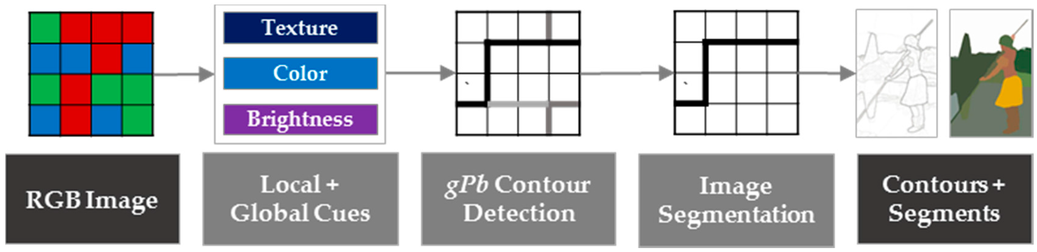
1.1. Contour Detection
1.2. Objective and Organization of the Study
2. Materials and Methods
2.1. UAV Data
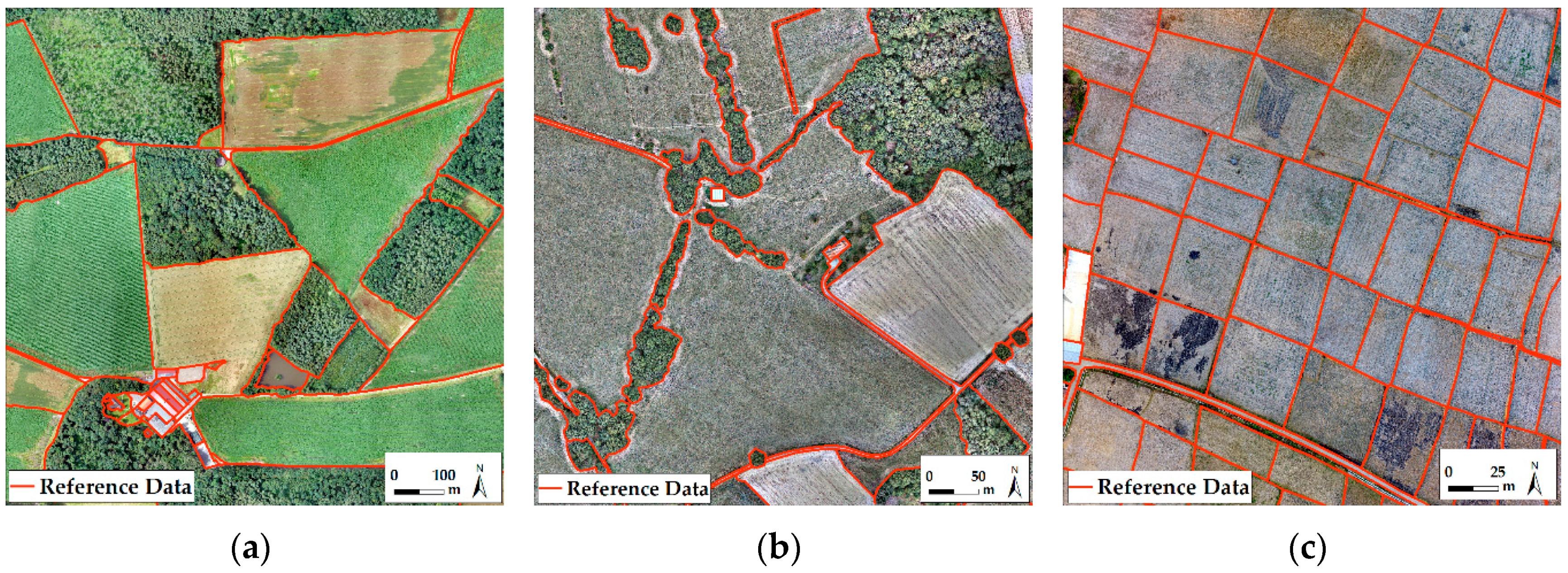
2.2. Reference Data
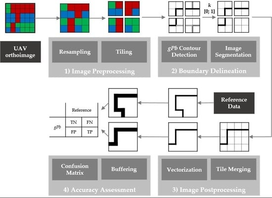
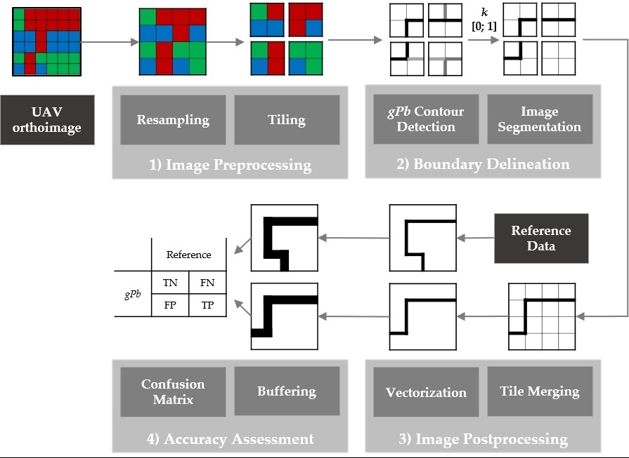
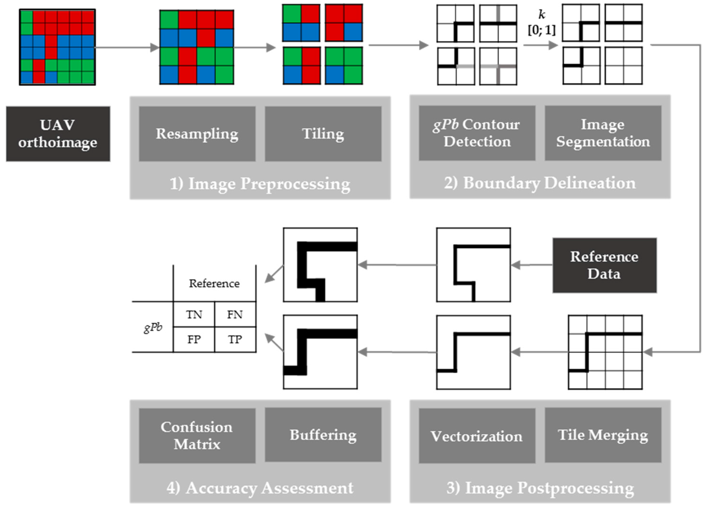
2.3. Image Processing Workflow
- (1)
- Image Preprocessing: The UAV orthoimage was first resampled to lower resolutions ranging from 5 to 100 cm GSD. All resampling was based on nearest neighbor resampling, as it is computationally least expensive. Initial tests with further resampling methods (bilinear, cubic, lanczos, average, mode) did not show significant differences in the gPb contour detection output. The resampling to different GSDs enabled investigation of the influence of GSD in detecting object contours. The resampled images of 1000 to 5000 pixels in width and height were then tiled to tiles of 1000 × 1000 pixels. The smaller the GSD, the more tiles were created (Table 2). The range of GSDs varied per study area, due to the varying extents per study area and the constant number of tiles amounting to 1, 9, 16 and 25 (Table 2): for Amtsvenn, the orthoimage covers an extent of 1000 × 1000 m, which results in a GSD of 50 cm, if the image is tiled to 4 tiles. The same number of tiles results in a GSD of 12.5 m for Lunyuk, since that orthoimage covers an extent of 250 × 250 m.
- (2)
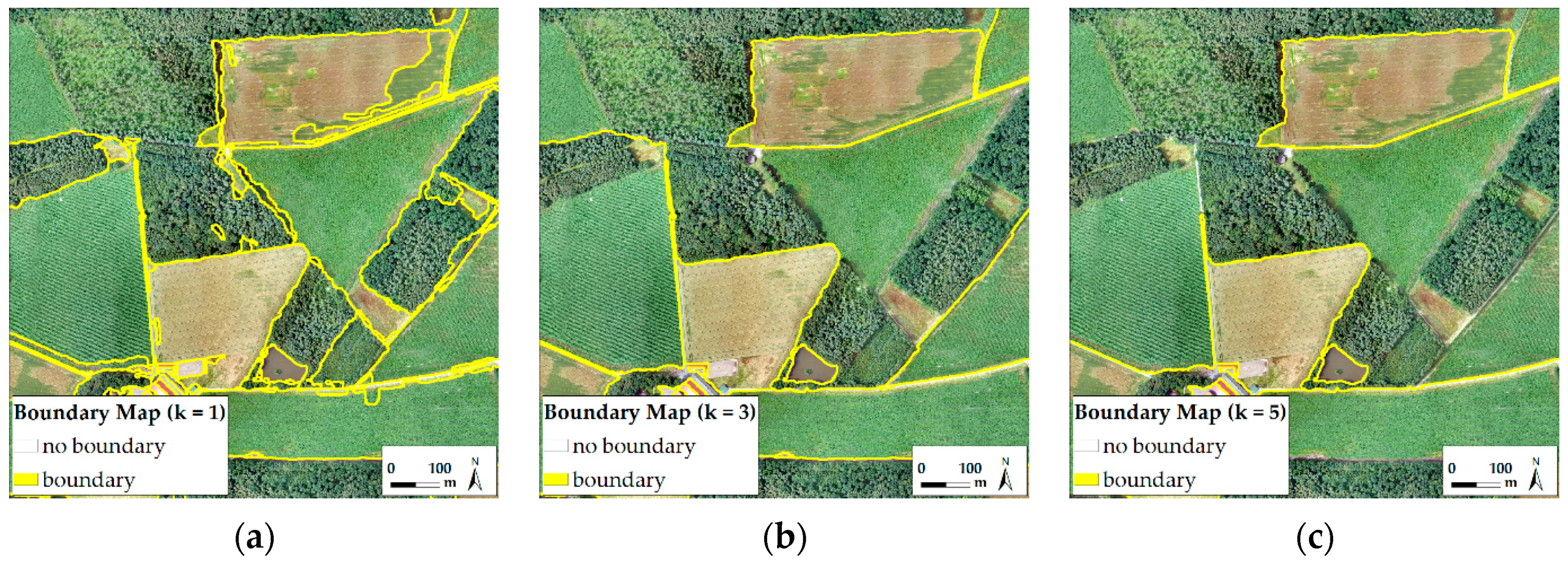
- Boundary Delineation: Then, gPb contour detection was applied to each tile of different GSDs. This resulted in contour maps containing probabilities for contours per pixel. By applying hierarchical image segmentation at scale k within the range [0; 1], contours of a certain probability were closed and transferred to a binary raster map containing pixels for the classes ‘boundary’ and ‘no boundary’. The resulting boundary map was created for all levels of k. This processing pipeline refers to gPb-owt-ucm, which is described in Section 1.1.
- (3)
- Image Postprocessing: All tiles belonging to the same set were merged to one contour map and one binary boundary map, which was then vectorized. This creates polygons for all connected regions of pixels in a raster sharing a common pixel value, which produces dense polygon geometries, with edges following exactly pixel boundaries.
- (4)
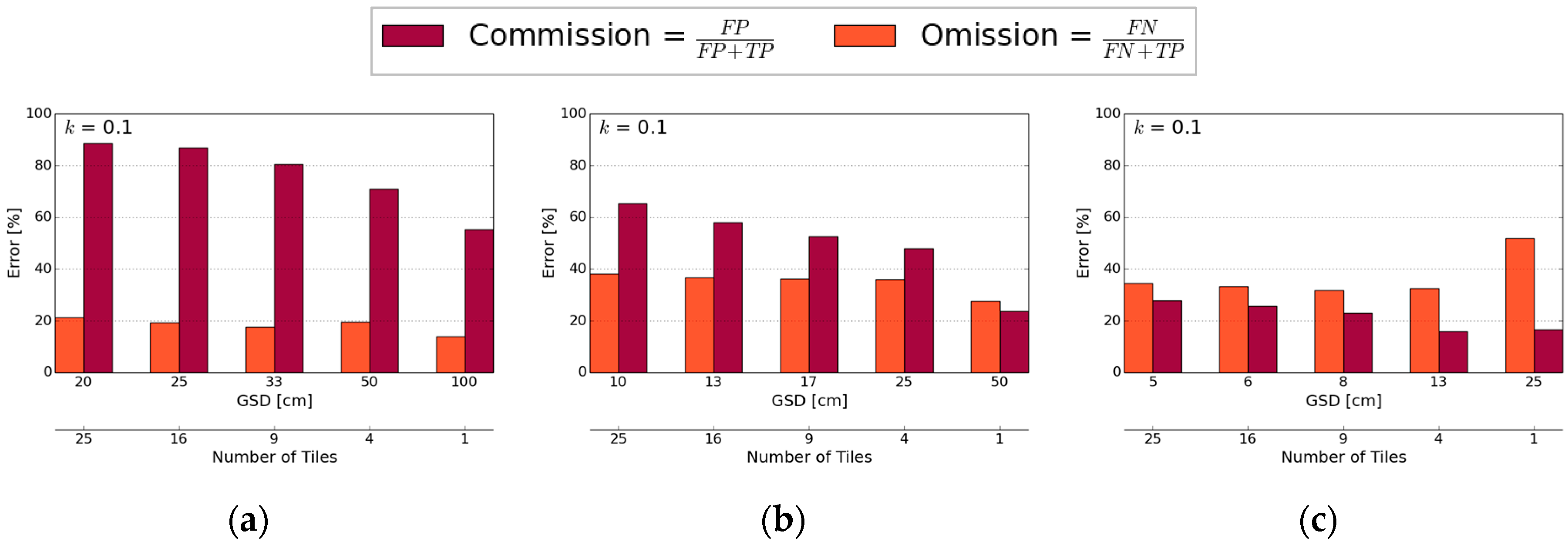
- Accuracy Assessment: The assessment was pixel-based and investigated the confusion matrix in terms of pixels labeled as true positives (TP), true negatives (TN), false positives (FP) and false negatives (FN) [34,35]. The accuracy assessment can equally be applied to a vector format by comparing the percentage of overlapping polygon areas per category. The accuracy assessment is designed to determine the accuracy in terms of (i) the detection quality, i.e., errors of commission and omission, and (ii) the localization quality, i.e., the accuracy of boundaries in a geometric sense:
- (i)
- For the detection quality, each line was buffered with a radius distance of 2 m and converted to a raster format. The same buffering and rasterization was applied to the reference data. From the confusion matrix, the following errors were calculated: the error of commission within the range of [0; 100], showing the percentage of pixels erroneously labeled as ‘boundary’ and the error of omission within the range of [0; 100], showing the percentage of pixels erroneously labeled as ‘no boundary’. A generous buffer of 2 m was chosen in order to account for uncertainties in conjunction with manual digitization and resampling effects.
- (ii)
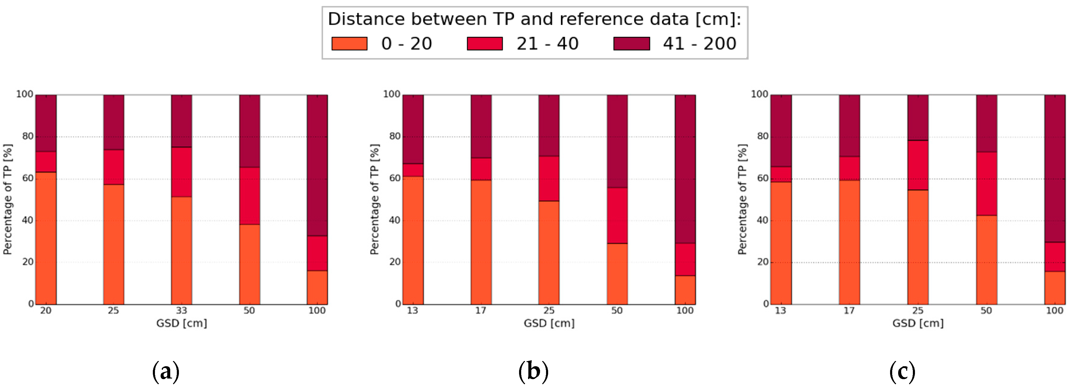
- Since multiple objects, such as trees and bushes, do not provide exactly localizable contours, the localization accuracy requires a different set of reference data. Therefore, a subset of the reference data was evaluated containing exactly locatable object contours only, i.e., road and roof outlines. This subset was rasterized to a raster of 5 cm GSD and each boundary pixel was buffered with distances from 0 to 2 m at increments of 20 cm. The binary boundary map was resampled to a GSD of 5 cm to be comparable to the reference raster. During the resampling, only one center pixel of 5 × 5 cm was kept per pixel of a larger GSD to avoid having a higher number of pixels after resampling a boundary map of a larger GSD. The resampled binary boundary map was then compared to the reference raster. Based on the confusion matrix, the number of TPs per buffer zone was calculated to investigate the distance between TPs and the reference data and thus the influence of GSD on the localization quality.
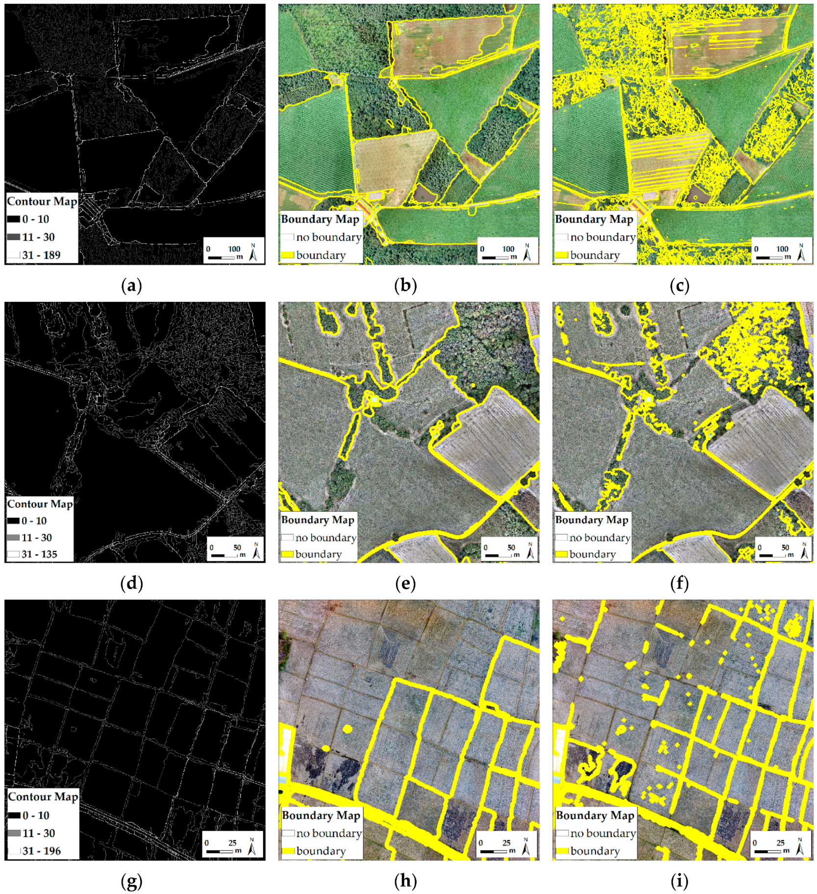
3. Results
4. Discussion
4.1. Detection Quality
4.2. Localization Quality
4.3. Discussion of the Evaluation Approach
4.4. Transferability and Applicability of gPb for Boundary Delineation
5. Conclusions
Acknowledgments
Author Contributions
Conflicts of Interest
Abbreviations
| DSM | Digital Surface Model |
| FN | False Negative |
| FP | False Positive |
| GCP | Ground Control Points |
| GNSS | Global Navigation Satellite System |
| gPb | Globalized Probability of Boundary |
| GSD | Ground Sample Distance |
| OWT | Oriented Watershed Transform |
| PPK | Post Processing Kinematic |
| TN | True Negative |
| TP | True Positive |
| UAV | Unmanned Aerial Vehicle |
| UCM | Ultrametric Contour Map |
References
- Colomina, I.; Molina, P. Unmanned aerial systems for photogrammetry and remote sensing: A review. ISPRS J. Photogramm. Remote Sens. 2014, 92, 79–97. [Google Scholar] [CrossRef]
- Nex, F.; Remondino, F. UAV for 3D mapping applications: A review. Appl. Geomat. 2014, 6, 1–15. [Google Scholar] [CrossRef]
- Pajares, G. Overview and current status of remote sensing applications based on unmanned aerial vehicles (UAVs). Photogramm. Eng. Remote Sens. 2015, 81, 281–329. [Google Scholar] [CrossRef]
- Manyoky, M.; Theiler, P.; Steudler, D.; Eisenbeiss, H. Unmanned aerial vehicle in cadastral applications. Int. Arch. Photogramm. Remote Sens. Spat. Inf. Sci. 2011, 63, 1–6. [Google Scholar] [CrossRef]
- Barnes, G.; Volkmann, W. High-resolution mapping with unmanned aerial systems. Surv. Land Inf. Sci. 2015, 74, 5–13. [Google Scholar]
- Mumbone, M.; Bennett, R.; Gerke, M.; Volkmann, W. Innovations in boundary mapping: Namibia, customary lands and UAVs. In Proceedings of the World Bank Conference on Land and Poverty, Washington, DC, USA, 23–27 March 2015; pp. 1–22.
- Volkmann, W.; Barnes, G. Virtual surveying: Mapping and modeling cadastral boundaries using Unmanned Aerial Systems (UAS). In Proceedings of the FIG Congress: Engaging the Challenges—Enhancing the Relevance, Kuala Lumpur, Malaysia, 16–21 June 2014; pp. 1–13.
- Maurice, M.J.; Koeva, M.N.; Gerke, M.; Nex, F.; Gevaert, C. A photogrammetric approach for map updating using UAV in Rwanda. In Proceedings of the GeoTech Rwanda—International Conference on Geospatial Technologies for Sustainable Urban and Rural Development, Kigali, Rwanda, 18–20 November 2015; pp. 1–8.
- Binns, B.O.; Dale, P.F. Cadastral Surveys and Records of Rights in Land Administration. Available online: http://www.fao.org/docrep/006/v4860e/v4860e03.htm (accessed on 10 November 2016).
- Williamson, I.; Enemark, S.; Wallace, J.; Rajabifard, A. Land Administration for Sustainable Development; ESRI Press Academic: Redlands, CA, USA, 2010; p. 472. [Google Scholar]
- Crommelinck, S.; Bennett, R.; Gerke, M.; Nex, F.; Yang, M.; Vosselman, G. Review of automatic feature extraction from high-resolution optical sensor data for UAV-based cadastral mapping. Remote Sens. 2016, 8, 1–28. [Google Scholar] [CrossRef]
- Jazayeri, I.; Rajabifard, A.; Kalantari, M. A geometric and semantic evaluation of 3D data sourcing methods for land and property information. Land Use Policy 2014, 36, 219–230. [Google Scholar] [CrossRef]
- Bennett, R.; Kitchingman, A.; Leach, J. On the nature and utility of natural boundaries for land and marine administration. Land Use policy 2010, 27, 772–779. [Google Scholar] [CrossRef]
- Zevenbergen, J.; Bennett, R. The visible boundary: More than just a line between coordinates. In Proceedings of the GeoTech Rwanda—International Conference on Geospatial Technologies for Sustainable Urban and Rural Development, Kigali, Rwanda, 18–20 November 2015; pp. 1–4.
- Canny, J. A computational approach to edge detection. IEEE Trans. Pattern Anal. Mach. Intell. 1986, 6, 679–698. [Google Scholar] [CrossRef]
- Malik, J.; Belongie, S.; Leung, T.; Shi, J. Contour and texture analysis for image segmentation. Int. J. Comput. Vis. 2001, 43, 7–27. [Google Scholar] [CrossRef]
- Martin, D.R.; Fowlkes, C.C.; Malik, J. Learning to detect natural image boundaries using local brightness, color, and texture cues. IEEE Trans. Pattern Anal. Mach. Intell. 2004, 26, 530–549. [Google Scholar] [CrossRef] [PubMed]
- Maire, M.; Arbeláez, P.; Fowlkes, C.; Malik, J. Using contours to detect and localize junctions in natural images. In Proceedings of the IEEE Conference on Computer Vision and Pattern Recognition, Anchorage, AK, USA, 23–28 June 2008; pp. 1–8.
- Arbelaez, P.; Maire, M.; Fowlkes, C.; Malik, J. Contour detection and hierarchical image segmentation. Pattern Anal. Mach. Intell. 2011, 33, 898–916. [Google Scholar] [CrossRef] [PubMed]
- Arbelaez, P.; Maire, M.; Fowlkes, C.; Malik, J. From contours to regions: An empirical evaluation. In Proceedings of the IEEE Conference on Computer Vision and Pattern Recognition (CVPR), Miami Beach, FL, USA, 20–25 June 2009; pp. 2294–2301.
- Arbeláez, P.; Fowlkes, C.; Martin, D. Berkeley Segmentation Dataset and Benchmark. Available online: https://www2.eecs.berkeley.edu/Research/Projects/CS/vision/bsds/ (accessed on 10 November 2016).
- Arbeláez, P.; Maire, M.; Fowlkes, C.; Malik, J. Contour Detection and Image Segmentation Resources. Available online: https://www2.eecs.berkeley.edu/Research/Projects/CS/vision/grouping/resources.html (accessed on 10 November 2016).
- Arbelaez, P. Boundary extraction in natural images using ultrametric contour maps. In Proceedings of the Conference on Computer Vision and Pattern Recognition Workshop (CVPRW), New York, NY, USA, 17–22 June 2006. [CrossRef]
- Jevnisek, R.J.; Avidan, S. Semi global boundary detection. Comput. Vis. Image Understand. 2016, 152, 21–28. [Google Scholar] [CrossRef]
- Zhang, X.; Xiao, P.; Song, X.; She, J. Boundary-constrained multi-scale segmentation method for remote sensing images. ISPRS J. Photogramm. Remote Sens. 2013, 78, 15–25. [Google Scholar] [CrossRef]
- Szeliski, R. Computer Vision: Algorithms and Applications; Springer: London, UK, 2010; p. 812. [Google Scholar]
- Dornaika, F.; Moujahid, A.; El Merabet, Y.; Ruichek, Y. Building detection from orthophotos using a machine learning approach: An empirical study on image segmentation and descriptors. Expert Syst. Appl. 2016, 58, 130–142. [Google Scholar] [CrossRef]
- Hou, B.; Kou, H.; Jiao, L. Classification of polarimetric SAR images using multilayer autoencoders and superpixels. IEEE J. Sel. Top. Appl. Earth Observ. Remote Sens. 2016, 9, 3072–3081. [Google Scholar] [CrossRef]
- Rottensteiner, F.; Sohn, G.; Gerke, M.; Wegner, J.D.; Breitkopf, U.; Jung, J. Results of the ISPRS benchmark on urban object detection and 3D building reconstruction. ISPRS J. Photogramm. Remote Sens. 2014, 93, 256–271. [Google Scholar] [CrossRef]
- QGIS Development Team. QGIS Geographic Information System; Open Source Geospatial Foundation: Chicago, CA, USA, 2009. Available online: www.qgis.osgeo.org (accessed on 21 June 2016).
- GRASS Developmnet Team. Geographic Resources Analysis Support System (GRASS) Software, Version 7.0. Available online: www.grass.osgeo.org (accessed on 21 June 2016).
- Conrad, O.; Bechtel, B.; Bock, M.; Dietrich, H.; Fischer, E.; Gerlitz, L.; Wehberg, J.; Wichmann, V.; Böhner, J. System for automated geoscientific analyses (SAGA) Version 2.1.4. Geosci. Model Dev. 2015, 8, 1991–2007. [Google Scholar] [CrossRef]
- GDAL Development Team. GDAL—Geospatial Data Abstraction Library, version 2.1.2; Open Source Geospatial Foundation: Chicago, CA, USA, 2016. Available online: www.gdal.org (accessed on 5 January 2017).
- Wiedemann, C.; Heipke, C.; Mayer, H.; Jamet, O. Empirical evaluation of automatically extracted road axes. In Empirical Evaluation Techniques in Computer Vision; IEEE Computer Society Press: Los Alamitos, CA, USA, 1998; pp. 172–187. [Google Scholar]
- Shi, W.; Cheung, C.K.; Zhu, C. Modelling error propagation in vector-based buffer analysis. Int. J. Geogr. Inf. Sci. 2003, 17, 251–271. [Google Scholar] [CrossRef]
- Mayer, H. Object extraction in photogrammetric computer vision. ISPRS J. Photogramm. Remote Sens. 2008, 63, 213–222. [Google Scholar]
- Kumar, M.; Singh, R.; Raju, P.; Krishnamurthy, Y. Road network extraction from high resolution multispectral satellite imagery based on object oriented techniques. ISPRS Ann. Photogramm. Remote Sens. Spat. Inf. Sci. 2014, 2, 107–110. [Google Scholar] [CrossRef]
- Goodchild, M.F.; Hunter, G.J. A simple positional accuracy measure for linear features. Int. J. Geogr. Inf. Sci. 1997, 11, 299–306. [Google Scholar] [CrossRef]
- Enemark, S.; Bell, K.C.; Lemmen, C.; McLaren, R. Fit-For-Purpose Land Administration; International Federation of Surveyors: Frederiksberg, Denmark, 2014; p. 42. [Google Scholar]
- Zevenbergen, J.; de Vries, W.; Bennett, R.M. Advances in Responsible Land Administration; CRC Press: Padstow, UK, 2015; p. 279. [Google Scholar]
- Mayer, H.; Hinz, S.; Bacher, U.; Baltsavias, E. A test of automatic road extraction approaches. ISPRS Int. Arch. Photogramm. Remote Sens. Spat. Inform. Sci. 2006, 36, 209–214. [Google Scholar]
- Basaeed, E.; Bhaskar, H.; Al-Mualla, M. CNN-based multi-band fused boundary detection for remotely sensed images. In Proceedings of the International Conference on Imaging for Crime Prevention and Detection, London, UK, 15–17 July 2015; pp. 1–6.


| Location | Latitude/Longitude | UAV Model | Camera/Focal Length [mm] | Overlap Forward/Sideward [%] | GSD [cm] | Extent [m] | Pixels |
|---|---|---|---|---|---|---|---|
| Amtsvenn, Germany | 52.17335/6.92865 | GerMAP G180 | Ricoh GR/18.3 | 80/65 | 4.86 | 1000 × 1000 | 20,538 × 20,538 |
| Toulouse, France | 43.21596/0.99870 | DT18 PPK | DT-3Bands RGB/5.5 | 80/70 | 3.61 | 500 × 500 | 13,816 × 13,816 |
| Lunyuk, Indonesia | −8.97061/117.21819 | DJI Phantom 3 | Sony EXMOR FC300S/3.68 | 90/60 | 3.00 | 250 × 250 | 8344 × 8344 |
| Pixels | Tiles | GSD (cm) Amtsvenn | GSD (cm) Toulouse | GSD (cm) Lunyuk |
|---|---|---|---|---|
| 5000 × 5000 | 25 | 20 | 10 | 5 |
| 4000 × 4000 | 16 | 25 | 12.5 | 6.25 |
| 3000 × 3000 | 9 | 33 | 16.5 | 8.3 |
| 2000 × 2000 | 4 | 50 | 25 | 12.5 |
| 1000 × 1000 | 1 | 100 | 50 | 25 |
| Amtsvenn | Toulouse | Lunyuk | ||||
|---|---|---|---|---|---|---|
| Pixels; GSD[cm] | 1000 × 1000; 100 | 1000 × 1000; 50 | 1000 × 1000; 25 | |||
| Tiles | 1 | 25 | 1 | 25 | 1 | 25 |
| Error of commission [%] | 55.15 | 70.01 | 23.43 | 53.88 | 17.21 | 31.10 |
| Error of omission [%] | 13.44 | 68.75 | 27.44 | 90.12 | 52.30 | 96.24 |
© 2017 by the authors. Licensee MDPI, Basel, Switzerland. This article is an open access article distributed under the terms and conditions of the Creative Commons Attribution (CC BY) license ( http://creativecommons.org/licenses/by/4.0/).
Share and Cite
Crommelinck, S.; Bennett, R.; Gerke, M.; Yang, M.Y.; Vosselman, G. Contour Detection for UAV-Based Cadastral Mapping. Remote Sens. 2017, 9, 171. https://doi.org/10.3390/rs9020171
Crommelinck S, Bennett R, Gerke M, Yang MY, Vosselman G. Contour Detection for UAV-Based Cadastral Mapping. Remote Sensing. 2017; 9(2):171. https://doi.org/10.3390/rs9020171
Chicago/Turabian StyleCrommelinck, Sophie, Rohan Bennett, Markus Gerke, Michael Ying Yang, and George Vosselman. 2017. "Contour Detection for UAV-Based Cadastral Mapping" Remote Sensing 9, no. 2: 171. https://doi.org/10.3390/rs9020171
APA StyleCrommelinck, S., Bennett, R., Gerke, M., Yang, M. Y., & Vosselman, G. (2017). Contour Detection for UAV-Based Cadastral Mapping. Remote Sensing, 9(2), 171. https://doi.org/10.3390/rs9020171