1. Introduction
For operational sea ice monitoring microwave sensors; such as synthetic aperture radar (SAR), scatterometer, and microwave radiometer, are mainly used as they can image sea ice through clouds and regardless of daylight conditions. SAR images are typically analysed visually by expert ice analysts or classified automatically into different ice types and open water, or sea ice parameters, such as sea ice concentration (SIC), stage of development, degree of ice deformation, etc. [
1,
2,
3]. The main usage of the microwave radiometer data has been the mapping of SIC, e.g., [
4,
5]. It has been also used for the estimation of snow thickness on sea ice and ice surface temperature, e.g., [
6], mapping of thin ice areas [
7,
8,
9] or estimation of thin ice thickness, e.g., [
10,
11]. Scatterometer data has been used for mapping of sea ice extent and ice edge location, and for sea ice typing [
12]. All of the sensors have been used for estimation of beginnings and endings of different sea ice thermodynamic regimes, e.g., [
12,
13,
14], and sea ice drift based on tracking of temporal changes in the imagery, e.g., [
12,
15,
16,
17].
For development and validation of sea ice retrieval algorithms for the microwave sensor data, independent sources of sea ice data are needed. The most accurate and detailed data are obtained by in-situ measurements, but they may be expensive to conduct and have typically limited spatial and temporal coverages. Airborne measurements with microwave sensors having similar properties as the satellite sensors and with supporting optical sensors are also very valuable. In recent years, the most extensive source of the airborne sea ice data in the Arctic has been the NASA’s Operation Ice Bridge (OIB) [
18]. The OIB measurements over sea ice are conducted only in the Western Arctic (from Greenland to Alaska), and mostly in spring (March-May). Currently, there is very little airborne data available over the Eastern Arctic, like the Kara Sea. Therefore, we would like to supplement the available in-situ and airborne sea ice data with an additional dataset having good spatial and temporal coverage. This can be derived from visible and thermal infrared (TIR) satellite imagery, although there are limitations due to the cloud coverage, daylight conditions, and quality of the derived sea ice products. Another option is to use fine resolution (<10 m) spaceborne SAR imagery and derived products, which show more details about spatial variation of sea ice properties, like degree of deformation, but these products themselves need validation, and the relationships between measured radar signatures and sea ice medium properties are equal to those in the coarser resolution radar data. The sea ice products that are derived from the visible and TIR imagery are largely independent of those from the microwave sensor data. Ice charts based on multisensor satellite data and manual data analysis methods can also be utilized, but the spatial resolution of the polygon-wise (containing ice attributes) charts is rather coarse, and the sea ice information in the form of the World Meteorological Organization (WMO) ‘egg code’ [
19] may require further processing for comparison with other sea ice products.
Visible and TIR satellite imagery have been used in many studies to aid in the development of the sea ice products from the microwave sensor data, and/or to evaluate their accuracy, e.g., [
9,
10,
11,
20]. In some studies, the visible and TIR imagery are just visually compared to the sea ice products, and the results are discussed in a more qualitative way. In more detailed studies, sea ice parameters, like ice extent or SIC, are retrieved from the visible and/or TIR imagery allowing for statistical comparisons between different sea ice products. Visible imagery have been used to derive pixel-based open-water classification, and further SIC estimates over larger areas, or pixel-based SIC, sea ice typing, sea ice albedo, melt pond fraction or thickness of snow-free thin ice (through relationships between sea ice reflectance spectra or albedo and thickness), e.g., [
20,
21,
22,
23,
24,
25,
26,
27,
28,
29]. TIR imagery acquired under cold winter conditions is first processed to the sea ice surface temperature (IST), and then the IST data are used to estimate either pixel-based SIC [
28,
29,
30,
31], detect leads [
32], or to estimate sea ice thickness (SIT) for thin ice (<50 cm; can be also snow covered), together with atmospheric forcing data on the basis of the surface heat balance equation, e.g., [
33,
34]. The IST based SIT estimation has many sources of uncertainty, like accuracy of the forcing data, cloud masking, and snow thickness on sea ice, but the SIT data has been found to be useful for the development of validation SIT retrieval algorithms for the microwave radiometer data [
10,
11], ice typing [
28], and for monitoring polynyas; their areas, SIT distributions, and ice production rates, e.g., [
35,
36,
37]. The maximum reliable retrieved SIT (set by some uncertainty level) has varied in different studies, e.g., 20 cm in [
37], 35–50 cm in [
34], and up to 100 cm in [
33].
There are not yet available well validated algorithms for retrieval of all sea ice parameters from the visible and IST imagery. The estimations of IST and open water–sea ice classification (i.e., sea ice extent) have likely the best maturity. However, the quality of all sea ice retrievals from the visible and IST imagery heavily depends on how well cloud masking has succeeded. In the case of the Moderate Resolution Imaging Spectroradiometer (MODIS) spectrometer imagery, the cloud masking typically has a good accuracy for polar daytime conditions when both reflectance and brightness temperature (
) data are available, but the performance is much poorer for polar night-time (only
data available) [
38,
39,
40,
41]. The detection of clouds in the polar region is inherently difficult due to poor visible reflectance and
contrasts between clouds and the underlying snow/ice surface. The undetected clouds in the Arctic are typically low-level (top height < 2 km) and high-level clouds (top height > 6 km), and, especially, those that are geometrically thin (<2 km) [
41]. In addition, the MODIS cloud detection algorithm severely underestimates cloud cover over sea ice [
41]. It is possible to evaluate the quality of the cloud mask in a sea ice product by its visual inspection against RGB-images from combinations of suitable reflectance and/or
bands. In addition, manual editing of the cloudmask has been conducted before the SIT estimation from the MODIS IST imagery [
34]. However, these methods are laborious and too time consuming for processing large datasets.
Currently, visible and TIR imagery (swath data) from many sensors, like MODIS and Visible Infrared Imaging Radiometer Suite (VIIRS), are used to generate operational sea ice products. The MODIS Sea Ice Product (MOD29) (1 km pixel size) contains IST in both daylight and night-time conditions, and sea ice extent under daylight only [
42]. Sea ice detection is achieved through the use of grouped criteria tests for sea ice reflectance characteristics in the visible and near-infrared (NIR) regions. VIIRS sea ice products (750 m pixel size) include IST, SIC, and sea ice age class (ice free, new/young ice (SIT < 30 cm), other ice) Environmental Data Records (EDRs) under both daytime and night-time conditions [
28,
43]. SIC is sea ice fraction in a pixel, and it is estimated using tie point signatures for open water and sea ice. The sea ice class in the night-time is estimated based on the IST and the surface heat balance equation [
33]. During the daytime, the ice age class estimation uses a modelled sea ice reflectance look-up-table (LUT). The ice age class product does not yet meet the set specification of 70% probability for correct classification [
28,
44]. These MODIS and VIIRS swath data sea ice products are also aggregated to daily gridded products, e.g., [
42].
Visual analysis of these operational MODIS and VIIRS sea ice products shows that there are many times cases of unmasked clouds that are classified as a sea ice parameter. Therefore, we think that these products cannot be used as comparison data for other sea ice products without their manual quality control and/or further processing.
Recently, new enhanced MODIS and VIIRS sea ice retrieval algorithms have been developed [
23,
29,
35], but by our estimation the resulting products are not optimal or accurate enough (e.g., due cloud masking errors) alone for the development and validation of the sea ice products from the microwave sensors. These new algorithms are reviewed in
Section 2.
In this paper, we have developed new algorithms and procedures to process a daily SIT chart and a daily open water–sea ice (OWSI) classification chart using the MODIS data. The daily SIT chart can be processed for winter (cold) night-time conditions, and the daily OWSI chart for daylight conditions. These charts are especially targeted for the development and validation of the sea products from the microwave sensors. In the development of the chart processing procedures, we targeted to reduce errors due to the undetected clouds, and to identify only larger cloud-free areas for the SIT and OWSI chart processing. Areas with tattered cloud mask, i.e., cloudy vs. cloud-free classification changes between neighbouring pixels, are not very useful for comparison with other sea ice products. The identification of larger cloud free areas is conducted by processing the original MODIS cloud mask, with 1 km pixel size to 10 by 10 km block size.
The daily SIT chart is based on all the available SIT swath charts calculated from the Terra and Aqua MODIS night-time IST data available in the MODIS Sea Ice Product (MOD29) [
42]. The SIT estimation is conducted, as in our previous study in [
34]. We enhance the cloud mask in the MOD29 IST imagery by using cloud cover data in the European Centre of Medium-Range Weather Forecast (ECMWF) ERA-Interim reanalysis data, and by further post-processing. The ERA-Interim cloud cover data has been used previously for the MODIS cloud mask improvement in e.g., [
35]. For determination of the algorithm for the additional cloud masking with the ERA-Interim data, we had a large dataset of manually cloud masked MODIS IST images for comparison.
The daily OWSI chart is processed from all of the available OWSI swath charts, calculated using only the MODIS 250 m (the best possible MODIS resolution) reflectance (
) data. For determination of the OWSI classification algorithm we had available MODIS
data manually selected from cloud masked false-color RGB imagery for open water and various sea ice types in late winter, early melt, and advanced melt conditions. The cloud mask here is based on the MODIS cloud mask product (MOD35 [
40]), with our new improvement to reduce false cloud detections over leads and polynyas.
In the following,
Section 2 first gives a review of recent developments in the MODIS and VIIRS sea ice retrieval algorithms. Next,
Section 3 describes our study area, the Barents and Kara Seas, datasets and their processing, and algorithms from our previous studies that are used in this paper. Our novel algorithms and procedures for calculating the daily SIT and OWSI charts from the MODIS data are presented in
Section 4. We present SIT charts that are calculated for the Barents and Kara Seas from a time period from November 2015 to April 2016, and OWSI charts for Mar to June 2016 in
Section 5. The accuracies of the SIT and OWSI charts are studied using ice charts that are produced by Arctic and Antarctic Research Institute (AARI) in Russia and Norwegian Meteorological Institute (METNO), respectively. We also conduct a comparison in the sea ice extent mapping between the thickness thresholded SIT chart and the OWSI chart. Both of the charts were processed for March to April 2016. Next, we demonstrate the usage of our charts for validation of a SAR and radiometer data based SIC product [
45]. In
Section 6 (Discussion), we compare our results to previous work, and finally, we give our conclusions in
Section 7.
2. Recent Previous Studies
In the following, recent developments in the MODIS and VIIRS sea ice retrieval algorithms are reviewed. We also evaluate their shortcomings in light of using the resulting products for the development and validation of the sea ice products from microwave sensors.
Paul et al. [
35] has presented new method for producing daily IST and SIT composites over polynyas, which includes usage of cloud cover information from the ECMWF ERA-Interim reanalysis data to complement the MODIS cloud mask [
40], assigning daily medians (from swath data observations) to IST and SIT, and a correction scheme for cloud-covered data. The IST and SIT composites are based on the night-time data only, which excludes uncertainties related to the effect of the solar shortwave radiation and surface albedo. Missing data in the daily IST and SIT composites due to cloud cover are complemented by a two-step procedure that comprises spatial feature reconstruction [
46] and proportional extrapolation [
47]. The spatial feature reconstruction is based on data acquired ±3 days around the day of interest and a SIT persistence index, which is the ratio of the number of swaths per pixel per day that contain thin ice (SIT ≤ 0.20 m) to the total number of clear-sky acquisitions. The proportional extrapolation assigns thin ice to cloud-covered areas in the same proportion as it is detected in the cloud-free area. These correction methods require setting up boundaries over targeted polynya regions. The resulting SIT charts have been used successfully to monitoring polynyas; their areas, SIT distributions, and ice production rates, both in the Arctic and Antarctic [
35,
36].
We think that these SIT charts are not optimal for monitoring thin ice areas within fast moving drift ice, or at rapidly changing ice edge, due to the cloud correction scheme that is based on data acquired within several days. In addition, for comparison with sea ice products based on SAR or radiometer swath data or their daily composites, we would like to identify automatically larger cloud-free areas and discard areas where the cloud mask is tattered.
An improved algorithm for mapping the sea ice extent using the MODIS visible and NIR imagery was recently presented by Gignac et al. [
23]. The algorithm denoted as IceMap250 has a decision tree approach that uses two different cloud masks to generate two intermediate open water–sea ice (OWSI) maps, both used in the end to create a composite OWSI map. The first cloud mask one is from the MOD35 cloud mask product [
40], and the second one, called the visibility mask, is from the thresholded normalized ratio between
’s at 3.7 (MODIS band 20) and 12 μm (band 32). The main goal of the visibility mask is not to detect clouds, but outline areas where open water may be detected, even though there are semi-transparent or thin clouds. The sea ice detection in based on a different spectral reflectance ratio and reflectance tests than in the MOD29 sea ice extent chart. The IceMap250 requires downscaling of the MODIS 500-m bands (bands 3–7) to the 250 m resolution of the bands 1 and 2. Validation the IceMap250 chart based on comparison with visually interpreted validation data showed a high classification accuracy (kappa values over 90%).
The IceMap250 seems a promising new algorithm for the MODIS based OWSI classification at 250 m resolution, but we think it has some properties that are not optimal for using it as comparison for the SAR based sea ice products. The downscaling of the MODIS 500 m data to the 250 m resolution may lead to some classification errors, as noted in [
23]. The OWSI classification algorithm was determined using manually selected MODIS
data samples for open water and sea ice in general (no ice typing). It would be good to also have
data statistics for various ice types. e.g., thin ice and heavily melt ponded ice, to study how they could change the thresholds in the IceMap250 OWSI classification. Identification of large cloud-free areas in the IceMap250 chart requires chart post-processing. Finally, the IceMap250 requires acquisition all MODIS L1B data files (at 250, 500 and 1000 m resolutions).
A new VIIRS algorithm for sea ice detection and further SIC mapping has been presented by Liu et al. [
29]. Sea detection in daytime is based on a spectral
ratio (0.86 and 1.6 μm; VIIRS bands M7 and M10), a single band
(0.86 μm) and IST, and in night-time on IST only. The SIC estimation in daytime in based on the visible
band at 0.67 μm and tie point reflectances for open water and sea ice with 100% SIC. For open water, the reflectance tie point has two different fixed values depending on the solar zenith angle range, but for sea ice the tie point reflectance is dynamic and determined locally. In night-time SIC is estimated using IST in a similar manner. The IST tie point for open water has only one fixed value. Daily SIC charts are composed by overlaying older cloud-free data with newer one. This VIIRS algorithm can also be applied to the MODIS data. The VIIRS SIC estimates were validated using SIC observations from the Landsat 8 imagery (30 m resolution). The VIIRS SIC had an overall bias of only −0.3% compared to the Landsat 8 SIC, and a precision of 9.5%. However, for the medium range SIC the differences were larger (e.g., bias −17% and precision 26% for the 30–50% SIC range), and they also depended on IST. These errors can be reduced with a tie point adjustment method applied for areas with leads, but this was concluded to require further studies.
For the pixel-based SIC estimation, the local determination of the sea ice tie point is certainly needed, but for the resulting tie point to be representative it requires that there are locally enough cloud-free sea ice pixels with 100% SIC, and that sea ice properties are locally rather homogeneous. The last requirement is not satisfied if the local area includes several ice types, like snow covered thick ice and snow-free thin ice, or mixture of melt ponded ice and ice without melt ponds. At the ice edge there may be no pixels at all with 100% SIC. Therefore, we suggest that currently the pixel-based SIC charts from the visible and IST data [
28,
29,
30,
31] are not yet accurate enough, especially in the mid-range of SIC (30% to 70%). It would be good to complement them with the SIC charts retrieved from the pixel-based OWSI classification of the visible and/or IST imagery by calculating fraction of sea ice pixels within radiometer footprints or segments of classified SAR images. The main drawback with this approach is that if there are a lot of detected sea ice pixels which are not truly 100% sea ice (mixed pixels), then SIC is overestimated.
The shortcomings of new MODIS and VIIRS sea ice products in a context of using them for the development and validation of sea ice products from microwave sensor data are summarized in
Table 1.
3. Materials and Methods
In this section, we first describe our study area, the Barents and Kara Sea, followed by the data sets that were used in our study and their pre-processing methods, and further, data processing methods and algorithms developed in our previous studies and utilized here. Various MODIS products are used as input data for the daily SIT and OWSI charts. The ERA-Interim reanalysis data is the external forcing data for solving SIT from the ice surface heat balance equation [
34], and for enhancing the cloud masking of the MODIS night-time IST data. For development of an algorithm for using the ERA-Interim cloud cover information in the cloud masking, we have a set of manually cloudmasked MODIS SIT images that are available from a previous study [
48]. Our OWSI classification algorithm is developed using a
dataset for various sea ice types selected from manually cloud masked MODIS RGB imagery. Ice charts by METNO and AARI are used for validation. Our experiment for using the daily OWSI and SIT charts in the validation of other sea ice products involves a SIC chart that is retrieved from the SENTINEL-1 SAR imagery and AMSR2 radiometer data [
45].
3.1. Study Area
Our study area in the Barents and Kara Seas is shown in
Figure 1. For the study area, we use a polar stereographic coordinate system with true scale latitude of 70N and mid-longitude of 55E. The size of the area is 2200 km (easting) by 1850 km (northing). Seasonal sea ice covers most of the study area. In the far north, however, multi-year ice (MYI) is present year-round [
49]. The average dates for the ice formation in the study area varies from 10 September in the far north to mid-November in the southern Kara Sea and south-eastern Barents Sea (Pechora Sea), and March–April in the central Barents Sea (west of Novaya Zemlya) [
49]. Melting of the sea ice begins in late April in the marginal ice zone of the Barents Sea. By the end of June, the central Barents Sea and the Pechora Sea are usually completely ice-free. In August, the ice edge reaches Svalbard and Franz Josef Land. In the Kara Sea, melting gradually starts in May and continues through July–August. Most of the Kara Sea is ice-free between mid-July and mid-August. In the Kara Sea, the ice season lasts for 6–9 months depending on the location and seasonal conditions.
3.2. MODIS Datasets and Processing
The MODIS spectrometer measures reflected solar and emitted thermal radiation in 36 spectral bands ranging from the visible to the TIR (0.415 to 14.235 μm) at spatial resolutions of 250 m (bands 1 and 2: 0.659 and 0.865 μm), 500 m (bands 3 to 7: 0.470, 0.555, 1.240, 1.640 and 2.130 μm), and 1 km (all others, including bands 31 (11.030 μm) and 32 (12.020 μm) that are used in the IST retrieval [
42]). The size of the MODIS L1B imagery is approximately 2030 km along track and 2330 km across track (swath width). The MODIS instrument is aboard NASA Terra and Aqua satellites. Following Terra MODIS products are used in the study here:
MOD02QKM-MODIS/Terra Calibrated Radiances 5-Min L1B Swath 250 m
MOD02HKM-MODIS/Terra Calibrated Radiances 5-Min L1B Swath 500 m
MOD021KM-MODIS/Terra Calibrated Radiances 5-Min L1B Swath 1 km
MOD03-MODIS/Terra Geolocation Fields 5-Min L1A Swath 1 km
MOD35_L2-MODIS/Terra Cloud Mask and Spectral Test Results 5-Min L2 Swath 250 m and 1 km
MOD29-MODIS/Terra Sea Ice Extent 5-Min L2 Swath 1 km
The same Aqua MODIS products are also used, but the prefix of the filename is MYD instead of MOD. In the following these products are only referred with the ‘MOD’ prefix. The MOD29 product was downloaded from the U.S National Snow and Ice Data Center (NSIDC), and all other products from the NASA Level 1 and Atmosphere Archive and Distribution System (LAADS), Distributed Active Archive Center (DAAC). The land mask for our study area was retrieved from the MOD44W (Land Water Mask Derived L3 Global 250 m) product available at the NASA Land Processes (LP) DAAC. The MOD29 product contains IST data and an OWSI chart based on reflectance tests. Under ideal conditions, clear sky with a low amount of water vapour, the MODIS IST accuracy is 1–3 K [
42,
50].
For calculation of the daily SIT chart, all available MOD29 products (only IST data used) for the study area shown in
Figure 1 were downloaded for 1 November 2015 to 30 April 2016. The daily OWSI chart is calculated using all available MOD02QKM products for 1 March to 30 June 2016. Both products are accompanied by the co-incident MOD03 geolocation product, and the MOD02QKM product also with the MOD35_L2 cloud mask product. The number of daily Terra and Aqua MODIS overpasses (some only very small spatial coverage) in the study area varied from 21 to 28.
We have previously produced a set of MODIS SIT charts for October 2014 to April 2015 [
48], see details in
Section 3.5. The cloud mask of the SIT chart, based on automatic cloud detection tests and further manual editing, is utilized in this study.
In the determination of the
statistics for open water and various sea ice types, we utilize a
dataset (MODIS bands 1–7) previously manually selected using cloud masked MODIS RGB imagery, see
Section 3.6. The input MODIS datasets here were MOD02, MOD03, and MOD35 products from the Terra MODIS. The time period of this data set is May to July 2009, and its coverage is mainly the Kara Sea.
The MOD02, MOD29, and MOD35 products were rectified to a polar stereographic (PS) coordinate system with true-scale latitude of 70 N and mid-longitude of 55 E (63 E for the 2009 data) using MODIS Swath Reprojection Tool available from the NASA LP DAAC. In the rectification, original pixel sizes (250, 500, or 1000 m) were kept. For all data, fixed PS grids (250, 500, or 1000 m) were used. The MODIS sensor and sun zenith () angles available in the MOD03 product were rectified to the pixel sizes of other products. The MODIS sensor scan angle () was calculated from the sensor zenith angle, Earth radius and satellite orbit altitude. Raw data from bands 1 to 7 were converted to top-of-the-atmosphere (TOA) sun angle corrected reflectances.
RGB-images were generated from different combinations of the
or
bands, e.g., RGB-image from bands 20-31-32 (3.750, 11.030, and 12.020 μm) and another one from bands 3-6-7 (0.470, 1.640, and 2.130 μm) for manual cloud masking of the MODIS night-time (
Section 3.5) and daytime (
Section 3.6) data, respectively. These RGB-images typically highlight well cloudy and cloud-free sea ice and open ocean areas.
The land mask of the study area for the MOD02 and data was processed from the MOD44W product with 250, 500, and 1000 m pixel sizes. Coastline was extracted from the land mask for the RGB-images. The MOD29 product already has a land mask.
In all MODIS data analyses here and in the retrieval of the daily MODIS SIT and OWSI charts
is limited to a maximum of 40° (the overall maximum is 55°). At
of 40° the MODIS spatial resolution in the across track direction decreases by a factor of around two [
51], e.g., from 250 m at nadir to ~500 m.
3.3. ERA-Interim Data
Numerical weather prediction model data over our study area were extracted from the ECMWF ERA-Interim reanalysis data. In the MODIS IST based SIT retrieval, the following ERA-Interim model parameters are used: air temperature and dewpoint temperature at 2 m height, wind speed
and
components at 10 m, mean sea level pressure, and downward longwave radiation. For further cloud masking of the MODIS IST data (night-time only) the ERA-Interim cloud cover data (total, high, medium and low cloud cover) are used. The time step of all data is 3 h and grid spacing is 0.25°. Over our study area the grid size is around 4–12 km along latitude and 28 km along longitude. The ERA-Interim data for the SIT retrieval were rectified to the same PS coordinate system as the MODIS data with the 1 km pixel size. The cloud cover data were rectified to a 10 km grid. All ERA-Interim data were further linearly interpolated to the acquisition times of the MODIS swath data sets, like in e.g., [
35,
36].
3.4. Sea Ice Thickness Estimation from MODIS IST Data
SIT from IST can be estimated on the basis of surface heat balance equation [
33]. Major assumptions here are that the heat flux through the ice and snow is equal to the atmospheric flux, and temperature profiles are linear in ice and snow [
33]. Our algorithm for the SIT estimation is described in detail in [
34]. Only night-time MODIS IST data are employed, and, thus, the uncertainties related to the effects of solar shortwave radiation and surface albedo are excluded. To simplify the SIT retrieval, we assume bulk of salinity of 9.2 ppt for sea ice, which corresponds to average salinity of sea ice with thickness of 20 cm [
52]. For snow thermal conductivity, we assume a constant climatological value of 0.31 W/m K
−1 as in [
33]. For bulk transfer coefficients for heat and evaporation a constant value of 0.003 is used. Previously in [
34], a simple linear parametrization between values for thin ice (0.003) and thick ice (0.00175) was employed, but according to [
37], a constant value of 0.003 is a good approximation for sea ice with SIT < 50 cm. For the SIT estimation for snow covered sea ice, a typical relationship between snow thickness and sea ice thickness is needed. It enables the conversion of a so-called thermal ice thickness (no snow cover assumed) from the heat balance equation to the ice thickness of snow covered ice. In [
34], this relationship was estimated based on that derived by Doronin [
53], and used in [
33], and on the Soviet Union’s Sever expeditions sea ice data [
54]. The resulting relationship was slightly discontinued at SIT of 20 cm. Here, we removed this discontinuity by following piecewise linear relationship:
where
is snow thickness and
is sea ice thickness.
A detailed study of the MODIS based SIT uncertainty was conducted in [
34] using data for three winters in 2008–2011 over the Kara Sea. In this study, the atmospheric forcing data were obtained from a numerical weather prediction model HIRLAM (HIgh-Resolution Limited Area Model). The typical maximum reliable SIT (max 50% uncertainty) was estimated to be 35–50 cm under typical weather conditions (air temperature
−20 °C, wind speed
5 m/s) that were present for the MODIS data. The accuracy is the best for the 15–30 cm thickness range, being around 38%. These figures were based on the Monte Carlo method, using estimated or guessed standard deviations and covariances of the input variables to the SIT retrieval. The largest SIT uncertainty came from
, and IST, and downward longwave radiative flux had somewhat smaller roughly equal contributions.
Undetected thin clouds and fog increase the SIT uncertainty. Undetected high thin clouds result in a cold bias in IST, making the sea ice appear thicker than it actually is. Ice fog that is generated by intense vapour flux from leads and polynyas under cold conditions is warmer than surrounding fast or pack ice IST, and is colder than IST for thin ice [
55]. This leads to SIT underestimation for pack ice and overestimation for thin ice.
The rather coarse resolution of 1 km for the IST data means that a pixel may cover mixture of sea ice types with variable thicknesses, i.e., so-called mixed-pixel effect. In this case, IST and estimated SIT are spatial averages for a 1 km pixel.
Our MODIS SIT retrieval algorithm is applied to the cloud masked IST swath data. The pixel size of the MODI SIT chart is 1 km and it shows SIT from 0 to 1 m and various masks, e.g., land and cloud masks. Retrieved SIT values over 100 cm are flagged as 100 cm, as for thick ice the SIT estimates have poor accuracy [
34]. The uncertainty of the retrieved SIT increases with increasing
, and therefore, the SIT retrieval is not conducted in conditions where
−5 °C. This
limit was based on the MODIS SIT uncertainty study conducted in [
34].
3.5. Manually Cloud Masked MODIS Night-time Data
Previously we have processed a set of 124 MODIS SIT charts for October 2014 to April 2015 [
48] for the study area shown in
Figure 1. We utilize here only the cloud mask of the SIT chart. It is used in development of an algorithm for improving the cloud mask in the MOD29 IST chart with the ERA-Interim cloud cover information.
The following method was used for the cloud masking of the night-time MODIS data [
34,
48]. Based on [
38,
39,
40] and our visual analysis of different cloud tests for the MODIS night-time data, we selected the following two cloud tests for the automatic cloud detection: (1) 11–3.9 μm brightness temperature difference (BTD) for low clouds; and, (2) 3.9–12 μm BTD for high clouds. The cloud tests are performed using non-overlapping 10 × 10 pixel blocks (10 by 10 km). If 10% (test 1) or 20% (test 2) of the block pixels are cloudy according to a cloud test, then the block is labelled as cloudy. Next, a morphological operation is performed to fill isolated small holes (clear sky). The results of the two cloud tests are then combined. Clear-sky restoration is conducted using 11 μm
, by reasoning that if under cold conditions it is over 272 K it represents cloud-free open water or very thin ice. Next, the following manual editing procedures can be conducted: filling holes, removing erroneous cloud mask elements, and masking arbitrary polygonal areas as cloudy or clear. The manual editing is conducted using two RGB-images (RGB-bands 20-31-32; and, (32-31)-(31-22)-31). Finally, the IST image is calculated and another round of manual cloudmask editing is conducted using the IST and the two RGB-images. Using 10 × 10 km blocks for the cloud mask, we can better identify large cloud-free areas and discard areas where the cloud mask is tattered. An example of the cloud mask is shown in
Figure 2.
3.6. Open Water and Sea Ice Reflectance Spectra from MODIS Data
In this paper, we develop an OWSI classification algorithm for the MODIS 250 m data (bands 1 and 2) using a TOA
dataset for open water and various ice types under late winter, early melt, and advanced melt conditions. The
dataset was constructed by selecting manually sample windows (3.5 by 3.5 km or 5.5 by 5.5 km) of different surface types from two MODIS RGB images, one from bands 3-6-7 and another one from bands 2-1-3. In the first RGB-image, sea ice and snow appear bright red and open water as black, and they are easily visually discriminated from clouds [
56]. The latter RGB image is suitable for the identification of melt ponded/wet sea ice, which can be identified by the bluish colour in the image. Melt ponds have relatively much higher
at the MODIS bands 1 and 3 than at the band 2 [
25] (
Figure 2 and
Table 1). The RGB-images were calculated from 34 cloud masked Terra MODIS swath datasets (L1B) acquired from 1 May to 17 July 2009, and covering mainly the Kara Sea. The
dataset includes the MODIS bands 1–7 and has 500 m pixel size. The dataset was prepared within an earlier unpublished study, and, therefore, the MODIS data is from an earlier year (2009) than the study period here.
Cloud masking of the MODIS datasets was conducted with similar methods as in
Section 3.5. Automatic cloud detection was performed using polar day cloud tests (in total four) from the MOD35 product [
40].
Over the RGB images sample windows were manually selected for open water and following sea ice types: snow covered thick first-year ice (TFYI) (thickness assumed to be over 30 cm), thin FYI (THFYI) (nilas and young ice, surface snow-free or thin snow cover; or, pancake ice) in winter (1–21 May 2009), and FYI covered with wet snow or early stage melt ponds (WETFYI) and melt ponded FYI (MPFYI) (likely snow mostly melted away) in summer (June–July 2009). The first three weeks of May 2009 still represented winter conditions, with dry snow pack. Early melting occurred around the first half of June, and advanced melting conditions (wet and melt ponded sea ice) likely were persistent after that. The sizes of the windows were 3.5 × 3.5 km for THFYI and MPFYI and 5.5 × 5.5 km for other surface types. The number of windows for each surface type varied from 86 for MPFYI to 809 for WETFYI. The maximum sun zenith angle is 67° in the winter data (May), and the average is around 58°. In the summer melting period data (June–July), the corresponding values are 58° and 51°, respectively.
The
spectra for the open water and winter ice types (TFYI and THFYI) are depicted in
Figure 3, and that for the open water and summer ice types (WETFYI and MPFYI) in
Figure 4. The
data can be used to study the discrimination of open water and sea ice, and different ice types using the MODIS single band
’s,
ratios (band A/band B) or normalized ratios ((band A–band B)/(band A + band B)).
Comparison of our average TOA
spectra in
Figure 3 and
Figure 4 to surface
spectra in [
25] (
Figure 2 and
Table 1) shows that their spectral behaviours follow each other quite closely, but there are differences in the
levels, especially at the band 2 for MPFYI here and young and mature melt bonds in [
25]. The surface
spectra in [
25] are for pure surface types, but our TOA
values, are affected by the mixed-pixel effect (a pixel has mixture of melt ponds and bare ice) and spatial variation of ice surface properties with the sample windows.
3.7. Daily Sea Ice Concentration Chart from AMSR2 Radiometer Data
A daily SIC product (level L3) over the Arctic from the Advanced Microwave Scanning Radiometer 2 (AMSR2) radiometer data is used to provide open water–sea ice classification (sea ice when SIC > 15%) for various studies here. The SIC product is freely available from the Japan Aerospace Exploration Agency (JAXA). The SIC estimation is based on the Bootstrap algorithm [
57]. The SIC chart is in the PS coordinate system with mid-longitude of 45 W and has pixel size of 10 km. The chart was interpolated to our study area by keeping the original 10-km pixel size.
3.8. METNO Ice Chart
The operational sea ice service at METNO produces a SIC chart that is based on a manual interpretation of satellite data [
58]. The SIC chart is a high resolution regional sea ice real-time product for the Svalbard and Barents Sea region covering an area from east Greenland to Novaya Zemlya. The chart does not cover the whole Kara Sea. Main satellite data source for the SIC chart is SAR imagery. Currently, SENTINEL-1 and RADARSAT SAR imagery are used. In addition to the SAR imagery, optical and TIR imagery from MODIS and Advanced Very High Resolution Radiometer (AVHRR), are used. A skilled ice analyst uses the latest available satellite data, and draws the ice chart in an ArcGIS production system. A new SIC chart is available every weekday at around 1400 GMT. The chart is in a PS coordinate system with true-scale latitude of 90 N, mid-longitude of 0 E, and spherical Earth datum. The pixel size of the chart is 1 km. The chart shows following SIC intervals of the WMO total concentration standard [
19]: very close drift ice (9–10/10), close drift ice (7–8/10), open drift ice: (4–6/10), very open drift ice (1–3/10), open water (<1/10), and ice free. The chart also shows areas of landfast ice, for which SIC of 10/10 is assigned.
The METNO SIC chart is available from Copernicus Marine Environment Monitoring Service (CMEMS) (see
http://marine.copernicus.eu/; product code: SEAICE_ARC_SEAICE_L4_NRT_OBSERVATIONS_011_002).
The SIC chart has been validated visually against optical imagery from AVHRR and MODIS [
59]. In addition, some alternative SAR imagery from COSMO-SkyMed SAR has been used. Generally, a good agreement was found between the chart and the optical and SAR imagery. The SIC chart has also been compared against manual ice chart by Danish Meteorological Institute (DMI) [
59]. The METNO and DMI charts have an overlapping area in the Greenland Sea. In general, there is in general a good consistency between the charts for the high SIC above 0.80. There is also, to a lesser extent, a good consistency between the charts when SIC is below 0.20. The SIC differences (up to 0.19 on the average) and standard deviations (up to 0.28) are highest for the intermediate SIC values. In general, the manual ice charts that are available through CMEMS are considered as the best available sea ice information, and are used as reference for other sea ice data sets [
59].
The METNO SIC chart is used for the validation of our MODIS based OWSI chart. The SIC charts were resampled into 250 m pixel size and cropped over our study area, see
Figure 5. In the validation, the SIC chart polygons are represented by a mid-value of the SIC range (except the open water class), i.e., the numerical SIC values are: 0.95, 0.75, 0.50, 0.20, 0.1, 0.0, and 1.0 for landfast ice.
3.9. AARI Ice Chart
AARI produces weekly ice charts for the Barents and Kara Seas [
60]. The charts show total concentration (code CT in [
19]) and partial concentrations of the first, second, and third thickest ice (codes CA, CB, and CC in [
19]), along with their respective stages of development (SA, SB, and SC) and form of ice (FA, FB, FC) for polygonal areas of variable sizes [
19]. The concentrations are shown with intervals of either 0.1 or 0.2 wide. The stage of development gives ice typing and following the thickness ranges are used: nilas (<10 cm), young ice (10–30 cm), grey ice (10–15 cm), grey-white ice (15–30 cm), thin FYI (30–70 cm), medium FYI (70–120 cm), thick FYI (≥120 cm), FYI in general (≥30 cm), and old ice (≥120 cm) [
19]. The form of ice shows e.g., ice floe size or occurrence of landfast ice. Some polygons only have one or two stage of development classes that are assigned to them (i.e., polygons are more homogenous). The ice charts are based on the available visible, TIR and SAR imagery and reports from coastal stations and ships. The polygonalization of images and subsequent interpretation and mapping of ice conditions are carried out by skilled ice analysts. The main purpose of the weekly ice chart is to show the spatial distribution and characteristics of sea ice. The AARI ice charts are in the digital SIGRID-3 vector file format [
61]. We have not found any publication that discusses the accuracy of the AARI weekly ice chart. The AARI ice charts are available through a web-site [
62].
The AARI ice charts are used for the validation of the MODIS SIT chart that is calculated for November 2015 to April 2016. The total number of the AARI charts for this period is 26 for both the Barents and Kara Seas. For the validation experiment polygons from an AARI chart were first gridded with 1 km pixel size to our study area, as shown in
Figure 1. Next, for each AARI ice chart polygon a mid-range SIC and mid-range SIT or upper or lower SIT values of the first, second, and third thickest ice types were assigned. However, for FYI in general type, a SIT value of 95 cm is used (same as for thick FYI). An average SIT for each chart polygon was calculated as a sum of the SIT values for the three ice types weighted with their SICs. Finally, the gridded charts for the Barents and Kara Seas were combined together, see an example in
Figure 6.
3.10. Sea Ice Concentration Estimation from SAR and Radiometer Data
We estimated SIC from SENTINEL-1 dual-polarized (HH/HV polarization combination) SAR and AMSR2 radiometer data by applying an algorithm developed in [
45]. The SIC estimation is based on a Multi-Layer Perceptron (MLP) neural network [
63] with SAR backscattering coefficients, several SAR texture features, and spectral gradient and polarization ratios that were computed from the AMSR2 multifrequency
data as its input (the algorithm is denoted here as AMSR2 + SAR SIC). The SIC estimates are computed for each SAR segment after a SAR segmentation phase with the Iterated Conditional Modes (ICM) algorithm [
64], i.e., the MLP inputs are segment-wise median values. The AMSR2 + SAR SIC algorithm was developed using data over the Baltic Sea for one whole ice season (2015–2016), and it is applied here over the Barents and Kara Seas without any modifications. For training the MLP digitized daily Baltic Sea ice charts that are produced at Finnish Meteorological Institute (FMI) by ice analysts were used. In the FMI ice charting process, an ice analyst identifies and indicates homogeneous ice areas by polygons and then attaches ice attributes such as SIC, minimum, average and maximum ice thickness and degree of ice deformation to each polygon. These are then digitized into a grid form with a 1 km grid cell size.
For comparison, we also estimate SIC based on the AMSR2 SIC data and SAR image segmentation (AMSR2 SIC + SAR segm.) [
65]. Here, AMSR2 gradient and polarization ratios alone are first used to estimate SIC with the MLP at the resolution of the AMSR2 data (around 10 km). Next, the SIC estimates are updated using the SAR segmentation by giving the SIC estimates as segment-wise medians. The resulting SIC is then given in the resolution defined by the SAR segmentation. The AMSR2 SIC + SAR segm. algorithm was also used as a reference algorithm in [
45].
The performance of these two SIC algorithms were evaluated in [
45] against an independent SIC dataset from the Baltic Sea ice charts. The mean absolute bias (L1 difference) was 6.7% for the AMSR2 + SAR SIC algorithm and 7.8% for AMSR2 SIC + SAR segm. The root-mean-square difference was 18.3% and 19.1%, respectively.
3.11. SENTINEL-1 SAR Imagery and AMSR2 Microwave Radiometer Data
The SENTINEL-1 SAR and AMSR2 radiometer data based SIC charts over the Barents and Kara Seas were calculated using 11 SENTINEL-1 Extra Wide (EW) Swath Mode SAR images that were covering the same time period as the MODIS SIT and OWSI charts. The SENTINEL-1 EW SAR images have HH/HV polarization combination and 40 by 40 m pixel spacing. A linear incidence angle correction [
66] was applied to the HH-polarization images, and a SAR noise correction algorithm [
67] to the HV-polarization images. Next, the SAR images were rectified to our PS coordinate system, with 100 m pixel size. Finally, a land mask for the AMSR-E radiometer data provided by NSIDC was applied to the SAR images.
The AMSR2 L1R (resampled swath data) data co-incident with the SENTINEL-1 SAR imagery was rectified to our PS coordinate system, with 1 km pixel size using bilinear interpolation.
5. Results
We present here SIT charts that are calculated for the Barents and Kara Seas from a time period of November 2015 to April 2016, and OWSI charts for March to June 2016. The accuracies of the SIT and OWSI charts are studied using the AARI and METNO ice charts, respectively. We also conduct a comparison in open water vs. sea ice mapping between the thickness thresholded SIT chart and the OWSI chart. Finally, we demonstrate the usage of the charts for validation of SENTINEL-1 SAR and AMSR2 radiometer data based SIC products [
45,
65].
5.1. Daily Sea Ice Thickness Chart
The number of the daily MODIS data acquisitions over our study area varied from 20 to 26, when counting also those with very small coverage. With the requirement of having at least 1000 pixels of SIT data in each SIT swath chart, the number of charts is highly variable, from 5 to 22, due to the variable degree of cloudiness. The average and modal amount of the charts for each day was 16 and 19, respectively. In March, and more in April, the number of swath charts and their coverage were also limited by the daylight conditions.
The areal coverage of the SIT data in the daily chart varies a lot from day to day due to the cloudiness. The average clear-sky fraction over ocean is only 14%, and 3/4 of fractions are below 17.5%. Against the sea ice area by the daily AMSR2 SIC charts (SIC > 15%), the daily SIT charts have sea ice coverage fractions from 0.02% to 72.6%, and the mean fraction is 28%. When dividing the fractions to 5% wide bins then the modal fraction is the 25–30% bin. Half of the fractions are below 27%, and further 3/4 of them are below 41%. These statistics show that typically the sea ice coverage in a daily SIT chart is moderate. In addition, sometimes the cloud cover in our study area is so persistent that a daily SIT chart contains too little SIT data for comparison with any other satellite data based sea ice product.
The number of SIT samples for a pixel varied from two to 14, the mean and modal values were only four and two, respectively. For 51% of pixels of all SIT charts, the number of samples was only either two or three, again due to the persistent cloudiness. At least two samples were required in the chart composition. Increasing the minimum number of required samples would increase the reliability of the SIT data, but this would significantly the decrease the spatial coverage of the daily chart.
Our visual analysis of the daily SIT charts showed that there are cases where some part of the chart has cloud contamination, see
Figure 16. The SIT chart for 23 January 2016 shows thick ice in the middle of the southern Kara Sea (between the Novaya Zemlya and the Yamal Peninsula), but on January 24, the chart shows instead a large area of thin ice (<25 cm) in the same location. This difference is very likely due to the undetected thin clouds or fog which have a higher temperature than IST for thick sea ice. An AARI ice chart (processed to average thickness for each polygon) on 26 January 2016 in
Figure 16c shows an average SIT of 30–40 cm for this area, and the dominant ice type is thin FYI (30–70 cm) with SIC of 50% or 70%. This points out the SIT chart on 23 January being more correct one. We conclude that manual quality control is needed for selecting the good quality charts (or chart areas) for comparison with other sea ice products.
As the SIT retrieval has many inaccuracies due to the inaccuracy of the forcing data and various parametrizations [
34], and the chart is showing daily median SIT, it is the best to use the chart for indication of various ice thickness categories, like 0.01–0.15 m, 0.16–0.30 m, 0.31–0.50 m and >0.50 m, or just for general open water, and thin (<0.30 m) and thick ice (>0.30 m) classes.
Validation with AARI Ice Chart
MODIS SIT charts for the same date and from the one day before and after were compared to an AARI ice chart. For the comparison each AARI chart polygon was classified into open water, thin ice (1–30 cm), thin FYI (30–50 cm), or thick FYI (>50 cm), according to the average SIT. For a AARI chart polygon that had at least 50% coverage in a MODIS SIT chart, the dominant ice class from the MODIS data was determined as following: first fractions of the four ice classes in the SIT data were calculated, and then the ice class which had the largest fraction, and having a value over 50%, was assigned. This 50% fraction threshold rejected polygons, which were too heterogeneous in the MODIS SIT data, which would make the determination of the dominant ice class too vague. The minimum required size for the AARI polygons used in the comparison was set to 100 pixels. MODIS SIT values less than 4 cm were assumed to represent open water. A slightly larger threshold than 0 cm was chosen due to the inaccuracies of the SIT retrieval and the daily SIT chart. Daily average air temperature () that was calculated from the ERA-Interim was used to study if the MODIS SIT chart accuracy is different in warm and cold conditions.
The results of the comparison are shown in
Table 2 in form of a contingency table. The MODIS SIT chart identifies correctly all open water polygons in the AARI ice chart. For thin ice the MODIS SIT chart accuracy against the AARI chart is only 44.5%, and 50.2% AARI thin ice polygons are classified as thick FYI. The number of pixel-wise SIT samples for the MODIS daily SIT chart is typically slightly larger in the correctly classified AARI thin ice polygons; the average is 4.8 and 64% of the polygon-wise averages are below 5, than in the polygons that are classified as thick FYI; the corresponding statistical figures are 4.0 and 77%. The miss-classification is more probable in warm weather conditions; for the miss-classified polygons
−10 °C in 24% of the cases, but only 9% for the correctly classified ones. Only 12% for the miss-classified polygons have
−20 °C, but for the correctly classified ones, this percentage is 38%. When in the chart comparison only those AARI chart polygons where the dominant ice type was a thin ice type (stage of development) with SIC > 70% were used then the classification accuracy was still only 46%, and again, 50% of the polygons were classified as thick FYI. Thus, the degree of homogeneity of the AARI chart polygons does not have significant effect on the thin ice classification accuracy.
Thin FYI class is not identified at all in the MODIS SIT chart, but is mostly identified as thick FYI (87.3% of cases). However, the original AARI ice chart itself does not use the thin FYI class, but the medium FYI category, which has a wider thickness range (30–70 cm). The thin FYI class here in the AARI chart results from the weighted averaging at maximum three stages of development classes. Therefore, we do not consider this mismatch as a serious defect. Nearly all (97.3%) thick FYI class polygons in the AARI chart were identified correctly in the MODIS SIT chart.
In summary, the MODIS daily SIT chart identifies correctly open water and thick FYI polygons of the AARI chart, but for the thin ice polygons, the classification accuracy is only around 45%, and the most common error (around 50%) is their classification as thick FYI. This classification error is slightly more common when the number of pixel-wise SIT samples in the daily SIT chart is small, and clearly occurs more often in warm weather conditions (
−10 °C). Typically, the accuracy of the retrieved SIT decreases as weather gets warmer, because the IST contrast between different ice thicknesses decreases [
34]. The SIT overestimation can also be due to inaccuracies in the atmospheric forcing data, e.g., a positive bias in
: now
IST for thin ice may resemble that of thick ice [
34]. The SIT overestimation also occurs when there is unmasked fog over thin ice in cold conditions [
34,
55] or snow thickness on sea ice estimated with (1) is too thin when compared to reality. Thus, there are many issues that can lead to SIT overestimation for thin ice, and which are mostly difficult to resolve. Finally, it is noted that the accuracy of the AARI ice chart is unknown, and that the chart has only a coarse ice thickness typing for large polygonal areas. For more accurate validation of the SIT chart measurements with airborne electromagnetic induction ice thickness instruments would be needed.
We suggest that the MODIS daily chart can be used as comparison data for sea ice products from the microwave sensor data, but as said previously, manual quality control (e.g., with the help of the MODIS RGB-images) is needed to select the best charts for comparison.
5.2. Daily Open Water-Sea Ice Chart
For the daily OWSI chart, the number of the MODIS data acquisitions over the study area for each day varied from 21 to 30. The number of daily OWSI swath charts with more than 16,000 pixels of OWSI data (ten 10 by 10 km blocks) varies from 6 to 22, and the mean and modal amounts are 16 and 20, respectively. The mean number of the charts for March is ten, but for the first two weeks, it is only seven. On 1 March, the daily OWSI chart can cover only the southern half of the study area (up around −1600 km in northing in
Figure 1) due to the daylight requirement of
80°. After around 30 March, the full coverage is possible. In May and June, the amount of the OWSI swath charts varies from 17 to 22, and the average is 20.
In the daily OWSI charts the average clear-sky fraction over ocean is only 18%, and 3/4 of fractions are below 23%. These figures are slightly larger than those for the swath SIT charts. The sea ice coverage fraction of the daily OWSI chart determined by the daily AMSR2 SIC chart (SIC > 15%) varies from 1.2% to 79.3%. The mean fraction is 31%, and the modal one is the 20–25% bin (with 5% wide bins). Half and 3/4 of the fractions are below 29% and 44%, respectively. The OWSI chart has slightly larger sea ice coverage than the SIT chart (mean coverage was 28%). The SIT chart coverage is not only limited by the cloudiness, but also by too warm conditions ( −5 °C), and by the requirement for having at least two pixelwise samples.
The number of samples for the OW class in the daily chart varied from one to 14. The mean and modal amounts were only three and one, respectively. For 55% of the OW class pixels, the number of samples was only either one or two. For the SI class, at least two samples were required, and the modal amount is the same as this minimum number. The mean number of samples was four, and the maximum was 14. The number of samples was only two or three for 48.5% of the SI class pixels. Like in the case of the daily SIT chart, there is a trade-off between the OWSI chart reliability and coverage.
Visual analysis of the OWSI charts indicated the need for manual quality control before their usage in further studies. However, as the OWSI chart derivation is much simpler than that of the SIT chart, the quality problems are not that severe.
Figure 17 shows two OWSI charts, one deemed to have good quality by visual analysis and by comparison to METNO ice chart in
Figure 17c, and one having an area where undetected clouds are assigned as SI class.
For the validation of the daily OWSI chart there are no in-situ and airborne data available. The chart accuracy is studied in next Section using the METNO ice chart. A validation study could also be conducted with fine resolution visible imagery, like with Landsat 8 (has bands with 15 and 30 m resolutions), as in [
29]. However, this study would be hampered by possible cloud masking defects in the fine resolution imagery, and an automatic or manual OWSI classification procedure would be needed for the imagery. The best usage of the fine resolution imagery would be to investigate the degree of the mixed-pixel effect on the OWSI classification.
Validation with METNO Ice Chart
The OWSI chart was compared against the METNO SIC chart from the same date in the following way: first SIC chart polygons, which have at least 50% coverage by the OWSI chart and are larger than 1600 pixels (equivalent to 100 1 km pixels), are found. Next, the SIC estimates from the OWSI chart for these polygons are calculated as fraction of sea ice pixels to the total number of pixels. Comparison SIC data from all of the chart pairs were combined together, and statistics (e.g., mean) for the MODIS SIC estimates for each SIC chart value (0.0, 0.1, 0.20, 0.50, 0.75, 0.95, and 1.0 for landfast ice) were calculated. Typically, many of the SIC chart polygons are very large, and thus, this 50% minimum coverage by the OWSI chart would rarely be fulfilled. Therefore, we included some fixed lines splitting the polygons to smaller ones in the SIC chart. The number of samples varies from 111 (SIC value of 0.0) to 1100 (SIC value of 0.20). The polygons for lower SICs are typically smaller than those for larger SICs, and thus, they often have over 50% coverage in the OWSI charts.
The results of the comparison are presented in
Figure 18. The variation of the MODIS SIC estimates for each METNO SIC chart value is large, e.g., for METNO SIC value of 0.50 the 10% and 90% percentiles are 0.07 and 0.98, respectively. However, the mean and median of the MODIS SIC estimates have an increasing trend with the increasing METNO SIC. The mean SIC is slightly larger at low and intermediate METNO SIC values (0.0 to 0.75); e.g., METNO SIC 0.20 vs. MODIS mean SIC 0.34, but at high SICs of 0.95 and 1.0 the relation is vice versa, e.g., METNO SIC 0.95 vs. MODIS mean SIC 0.89. At low and high METNO SICs, the MODIS median SIC is close to them.
We think that large MODIS SIC variation can be explained by the different properties of the two charts. The METNO chart shows SIC estimates with a SIC range of only 0.1 or 0.2 for large polygonal areas. The SIC estimates are based on the visual analysis of mainly SAR imagery, and also on cloud-free optical and TIR imagery, when available [
58]. By our experience visual detection of small open water leads and polynyas (<few kms) is typically difficult in SAR imagery, and depends on wave conditions (i.e., wind and fetch). Whereas, the OWSI chart can detect these in the 250-m scale. Therefore, the METNO chart shows an average SIC for a large area, but locally, SIC can be larger or smaller, and this can be detected by the OWSI chart. In addition, the sizes of the METNO chart polygons have an effect on the comparison results, especially for landfast ice. Some landfast ice polygons are small and next to open water (e.g., in the Pechora Sea, see
Figure 1). In this case co-location errors of the two charts can lead to large differences between the SIC estimates. The landmasks in the two charts do not coincide exactly. When we increase the minimum acceptable METNO chart polygon size to tenfold (to an area of 1000 1 km pixels) then the MODIS SIC variation decreases, and the mean and median SICs are closer to the METNO SICs, e.g., now we have METNO SIC 0.20 (0.95) vs. MODIS mean SIC 0.24 (0.94), and for landfast ice the mean SIC increases from 0.76 to 0.85. Further tenfold increase of the minimum polygon size gives the mean MODIS SIC of 0.93 for landfast ice, and only two SIC samples are below 0.8 (in total 32 samples).
We conclude that the OWSI chart on the average gives SIC estimates following those in the METNO ice chart. Further studies with a fine resolution (<50 m) OWSI or SIC charts from airborne or satellite optical imagery would be needed for a more detailed accuracy evaluation.
5.3. Comparison of MODIS SIT and OWSI Charts
The daily SIT and OWSI charts were compared to each other in open water–sea ice classification during a period of March to April 2016. For the comparison the SIT chart was processed to a pixel based OWSI classification by assuming that SIT values less than 4 cm represent open water. This chart is denoted here as the SIT-OWSI chart. The OWSI chart with the 250 m pixel size was processed to 1 km pixel size (denoted as OWSI-1 chart) by assigning OW (or SI) class to a 1 km pixel if its area contained at least twelve 250 m OW (or SI) pixels (75% of all pixels). The comparison of the SIT-OWSI and OWSI-1 charts was conducted over pixels which were either OW or SI class in both charts. The total number of these pixels is large, around 13.7 × 10⁶. Unfortunately, the SIT-OWSI charts do not often show open water next to the ice edge due to the cloud mask.
Table 3 shows contingency table from the pixel-wise comparison of the charts. The SIT-OWSI and OWSI-1 charts agree very well in the detection of OW and SI; 99.5% of the pixels are labelled with the same class. The case where the OWSI-1 charts show SI, but the SIT-OWSI shows OW (percentage of these pixels is 0.33%) is around two times is more common than the opposite case (0.17%). Within single chart pairs, the equivalence between the pixels varies from 84.7% to 100%, but it is mostly above 98%.
This high agreement between the two charts gives further confidence on the reliability of our algorithms and procedures for the MODIS SIT and OWSI chart processing. It is noted that the two charts are fully independent in the estimation of the sea ice properties.
5.4. Validation of SAR and Microwave Radiometer Based Sea Ice Concentration Chart
SIC charts were calculated from the SENTINEL-1 SAR and AMSR2 radiometer data, with two different algorithms: A1 is SIC with the MLP having as inputs SAR segment-wise median AMSR2 and SAR features [
45] (shortly SAR + AMSR2 SIC), and A2 is SIC first with the MLP having only the AMSR2 polarization and gradient ratios as inputs, and then the SIC estimates are updated using the SAR segmentation [
65] (AMSR2 SIC + SAR segm.); for details see
Section 3.10. Both of the algorithms were trained for the Baltic Sea. We use currently A1 for operational sea ice monitoring. The older algorithm A2 was included here for reference and comparison. The total number of the SIC charts with both algorithms is 11.
The SIC charts based on the SENTINEL-1 and AMSR2 data were compared to the co-incident SIC data derived from the MODIS daily OWSI and SIT charts. The SIC data from the MODIS OWSI charts was obtained by counting the number of open water and sea ice pixels for each SAR segment, and computing SIC as a ratio between the sea ice pixels and the total number of pixels. The MODIS SIT charts were first classified to open water and sea ice pixels using again the 4 cm thickness threshold, and then the SIC estimates for the SAR segments were calculated. The agreement between the two SIC datasets is characterized with the following statistics: mean bias, mean absolute bias (L1 difference; shortly L1d), root-mean-square difference (RMSD), and coefficient of determination ().
The validation results for the two different SENTINEL-1 and AMSR2 SIC charts calculated with the SIC data from the MODIS OWSI charts (March, May and June 2016) are shown in
Table 4. A SAR + AMSR2 SIC chart and corresponding MODIS SIC chart (SAR segment-wise SIC) is shown in
Figure 19. For April 2016 there was no co-incident SIC charts and cloud-free MODIS data. The amount of co-incident data was the largest for June 2016. The results suggest a good accuracy for the SAR + AMSR2 SIC chart, RMSD is only 11.5%, and L1d is only 5.4%, and
is high, 0.91. The match between the SAR + AMSR2 SIC and MODIS SIC charts is good in
Figure 19. The L1d and RMSD statistics are only slightly worse for the AMSR2 SIC + SAR segm. chart. The mean bias is very small for both SIC charts, below 2%.
Table 5 shows validation statistics based on the MODIS SIC data calculated from the MODIS SIT charts. Again, the results indicate good accuracy for the two SIC charts. Here, L1d and RMSD are slightly smaller for the AMSR2 SIC + SAR segm. chart, but
is higher for the SAR + AMSR2 SIC chart.
It is notable that the RMSD values in
Table 4 and
Table 5 are lower than those for the Baltic Sea SIC charts in [
45], even though the two SIC algorithms were trained with the Baltic Sea ice data. This may be due different type of validation data used in [
45]; SIC estimates from manually prepared ice charts in [
45] vs. much finer resolution MODIS SIT and OWSI charts in here.
We think that the results of this validation experiment shows the applicability of the SAR + AMSR2 SIC and AMSR2 SIC + SAR segm. algorithms that are trained for the Baltic Sea, also for the Barents and Kara Seas. It was not possible to determine which algorithm is the best one. Further work is needed for training of the algorithms for all seasonal ice conditions, from sea ice freeze-up to advanced melting, and to study dependence of errors on weather and sea ice conditions (e.g., different ice types, melting ice). The training can be conducted using the MODIS OWSI and SIT charts covering 2–3 ice seasons. MODIS charts from one ice season alone may not cover all different weather and sea ice conditions as the chart coverage is significantly restricted by the clouds.
6. Discussion
The accuracy of the cloud masking was found to be one of the main issues for the usability and accuracies of the MODIS SIT and OWSI charts. Thus, we concluded that manual quality control is needed for selecting the good quality charts (or chart areas) for comparison with other sea ice products. However, this process can be conducted with a little effort, even for a large set of daily charts, like covering one sea ice season.
Recently, Paul et al. [
35] presented a new kind of daily SIT chart, which have been used in studies of the Arctic and Antarctic polynyas [
35,
36]. The chart includes the correction of the cloud covered areas, which is a good feature when you want to detect polynyas and monitor their temporal and spatial dynamics, but due to this correction, we think that these charts are not optimal for monitoring thin ice areas within drift ice or at rapidly changing ice edge. Overall, our daily SIT chart processing method and that by Paul et al. [
35] differ in cloud masking, and in the processing of the daily SIT information from the swath data observations. We suggest that our daily SIT chart and that by Paul et al. [
35] can supplement each other in monitoring of the Arctic sea ice. We found out that the OWSI classification in daytime can be simply conducted with high accuracy using only the MODIS band 1 reflectance (
) thresholding. In the training, MODIS
data set the OW and SI miss-classification percentages were below 0.5%. The
imagery has the best possible MODIS resolution of 250 m. Previously also, another simple algorithm, the reflectance ratio (
) between bands 1 and 2 has been used for the OWSI classification [
69,
70]. We found that this ratio is sometimes contaminated by a detector striping artefact (see [
71]) in the
image which leads to false SI detection. Under winter conditions, discrimination between THFYI and TFYI seems to be possible, but we think further studies are needed to confirm this, and to study also the mixed-pixel effect in the classification. How well very thin ice (<5 cm) is discriminated from OW is also currently unknown. A major flaw in the MOD35 cloud mask was found: false cloud detection over cloud-free leads and polynyas with open water or thin ice surface due to a coarse resolution sea ice product used to initialize the sea ice background flag for the MODIS cloud mask algorithm processing flow [
42]. We developed a clear-sky restoration algorithm to compensate this error. It seems that this cloud mask error has not been taken into account in previous MODIS sea ice classification studies.
Recently introduced IceMap250 algorithm by Gignac et al. [
23] also produces the OWSI classification at the 250 m resolution. This algorithm is more complex than ours and requires the acquisition of all MODIS L1B data files (at 250, 500, and 1000 m resolutions). The IceMap250 uses a clever way to detect OW through semi-transparent or thin clouds, which increases both the coverage of the OWSI chart and its confidence. Unlike our algorithm the IceMap250 has a dynamic threshold in the OWSI classification adapting to different seasonal sea ice conditions. Analysis of our MODIS
data for OW and various ice types in different seasonal conditions showed that a fixed
threshold is enough to give an accurate OWSI classification. We suggest that a comparison study between the IceMap250 and our OWSI algorithm should be conducted to see their pros and cons, and for any further developments, like merging of the two algorithms. Currently, both of the algorithms slightly overestimate the sea ice extent due to the mixed-pixel effect.
The
(daytime) or IST (night-time) data have also been used for the pixel-based SIC estimation [
28,
29,
30,
31]. This requires open water and sea ice (100% SIC) tie points. The sea ice tie point is determined from local
or IST statistics, and for open water, fixed tie point values are used. The resulting sea ice tie point is representative only when there is enough cloud-free sea ice pixels with 100% SIC, and when sea ice properties are locally homogeneous. In the [
29], the accuracy the SIC estimation with the VIIRS data (both
and IST) was found to be good by comparison to Landsat 8 SIC retrievals, but the accuracy was rather poor in the mid-range of SIC, (from 15% to 70%), and it also depended on IST. The SIC estimation with IST has inherently poor accuracy in warm conditions as the difference between IST and sea surface temperature is small, and the accuracy of the IST measurement itself starts to have a large role in the accuracy of the estimated SIC [
34,
50]. We prefer to use the night-time IST for the SIT estimation, as data on thin ice thickness is valuable in the development and validation of many sea ice products, like thin ice detection and thickness estimation with microwave radiometer data, e.g., [
9,
10,
11]. In the SIT estimation, we have an air temperature limit (−5 °C), above which the SIT retrieval is not conducted [
34].
We think that the pixel-based SIC chart that is presented in [
29] is not yet accurate enough to fully develop and validate SIC charts from the SAR and microwave radiometer data. Therefore, it would be good to complement it with our daily OWSI chart in the development and validation of other SIC charts. We also propose to study if the MODIS 250 m data alone can be used for reliable pixel-based SIC estimation, following the algorithm in [
29].
The accuracies of the MODIS SIT and OWSI charts were studied using the AARI and METNO ice charts, respectively. The SIC estimates from the OWSI chart were found to follow on the average those in the METNO ice chart. We also discussed issues that contribute to a large discrepancy sometimes found between the SIC estimates from the two charts. Open water and thick ice FYI polygons were correctly identified by the SIT chart, but for thin ice polygons the classification accuracy was only around 45%, and the most common error (around 50%) was their classification as thick FYI. This classification error was found to be more common in warm weather conditions ( −10 °C). Other issues that lead to SIT overestimation for thin ice were also identified, like assuming too thin snow cover on thin ice in the SIT retrieval (see (1)). In general, these issues are difficult to resolve and require further studies.
The pixel-wise cross-comparison of the daily SIT and OWSI charts showed very good agreement in open water vs. sea ice classification. We think that this gives further confidence on the reliability of our MODIS algorithms.
For further studies on the accuracy of the charts, we would need fine resolution independent sea ice data from satellite or airborne measurements.
When analysing our MODIS
data set for OW and various ice types, we observed an unnecessary element in the sea ice detection algorithm of the MODIS Sea Ice Product (MOD29) [
21,
22,
42]. The sea ice detection rule there is that NDSI between bands 4 (0.555 μm) and 6 (1.6 μm) must be larger than 0.4, and
and
. In our data, NDSI was always larger than 0.4 for all surface types, see
Figure 20. Thus, the sea ice detection is really based only on
and
. NDSI was originally developed for detection of snow over on land, and it separates snow covered and snow-free non-densely forested regions [
72,
73]. It is noted that we also use
for the sea ice detection.
7. Conclusions
We have developed algorithms and procedures for calculating daily SIT and OWSI charts based on the MODIS IST (night-time) and reflectance (daytime) swath data, respectively. The target area for the charts is the Barents and Kara Seas, but the charts can be processed for other Arctic Ocean areas after some minor modifications in the algorithms. The charts are targeted to be used in development and validation of sea ice products from swath or daily aggregated microwave sensor data. Therefore, our cloud masking focus on identifying large cloud-free areas in the MODIS swath data, and no supplementation of cloud covered areas in the daily charts using data from several days, as in [
35], is conducted. Unfortunately, the cloud masking of the MODIS daytime, and, especially, the night-time swath data is challenging [
38,
39,
40,
41], and cases of miss-detected clouds or sea ice classified as cloud occurs. Thus, manual quality control is needed for selecting the good quality charts (or chart areas) for comparison with other sea ice products, but this process can be conducted with a little effort.
The SIT estimation from the MODIS IST swath data is based on previous studies [
33,
34], and we focused here on enhancing the cloud mask of the MODIS night-time data with the help of the ERA-Interim cloud fraction data, and further processing of the cloud mask (from 1 to 10 km pixel size). The daily SIT chart is composed from available swath charts by assigning daily median SIT to a pixel, if there was at least two SIT samples. This procedure somewhat compensates errors due to the undetected clouds in the swath SIT charts.
For the development of the OWSI classification algorithm for the MODIS
data at the 250 m resolution, we utilized MODIS
data manually selected for open water and various sea ice types in late winter, early melt, and advanced melt conditions. Analysis of the
data showed that very accurate OWSI classification is possible using only a simple fixed thresholding of the MODIS band 1 reflectance (
). The cloud masking of the
data is based on the MOD35 product [
40], our new algorithm for clear-sky restoration over leads and polynyas, and post-processing of the resulting cloud mask to the 10 km pixel size. The daily OWSI chart is calculated from all the available MODIS swath charts with a set of rules that correct for false detections of SI in the swath charts due to the undetected clouds.
The SIT and OWSI charts were compared against the AARI and METNO ice charts, respectively. On average, a good relationship between the charts was found, but there was also cases of noticeably mismatch, especially in the identification of thin ice polygons in the AARI chart succeeded only with 45% accuracy. Plausible reasons for these mismatches were identified, and some of them may be resolved with further studies. Pixel-wise cross-comparison of the SIT and OWSI charts showed very good agreement in open water vs. sea ice classification which gives further confidence on the reliability of our MODIS algorithms.
We suggest that these new daily MODIS OWSI and SIT charts can supplement other MODIS sea ice products (sea ice extent, SIC, and SIT) [
23,
28,
29,
35,
42] in the Arctic sea ice monitoring, and especially, in the validation and development of sea ice products from the microwave sensor data.
There are several topics for further research, including to study whether it is possible to discriminate thin and thick FYI with in late winter, estimate pixel-based SIC with , increase the accuracy of the SIT retrieval for thin ice, or merge our algorithms with previous ones for better accuracy in the SIC or SIT retrieval. The mixed-pixel effect in the SIT retrieval and OWSI classification should also be investigated.
We successfully demonstrated the usage of the MODIS OWSI and SIT charts for the validation of SIC charts based on the SENTINEL-1 SAR and AMSR2 radiometer data and two different algorithms [
45,
65]. The validation experiment showed the applicability of the two SIC algorithms trained for the Baltic Sea, also for the Barents and Kara Seas. Further work needs to be conducted for fine tuning the algorithms for the Barents and Kara Seas, and for all possible weather and ice conditions, i.e., a representative training data set is required.


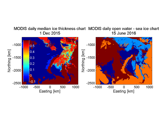
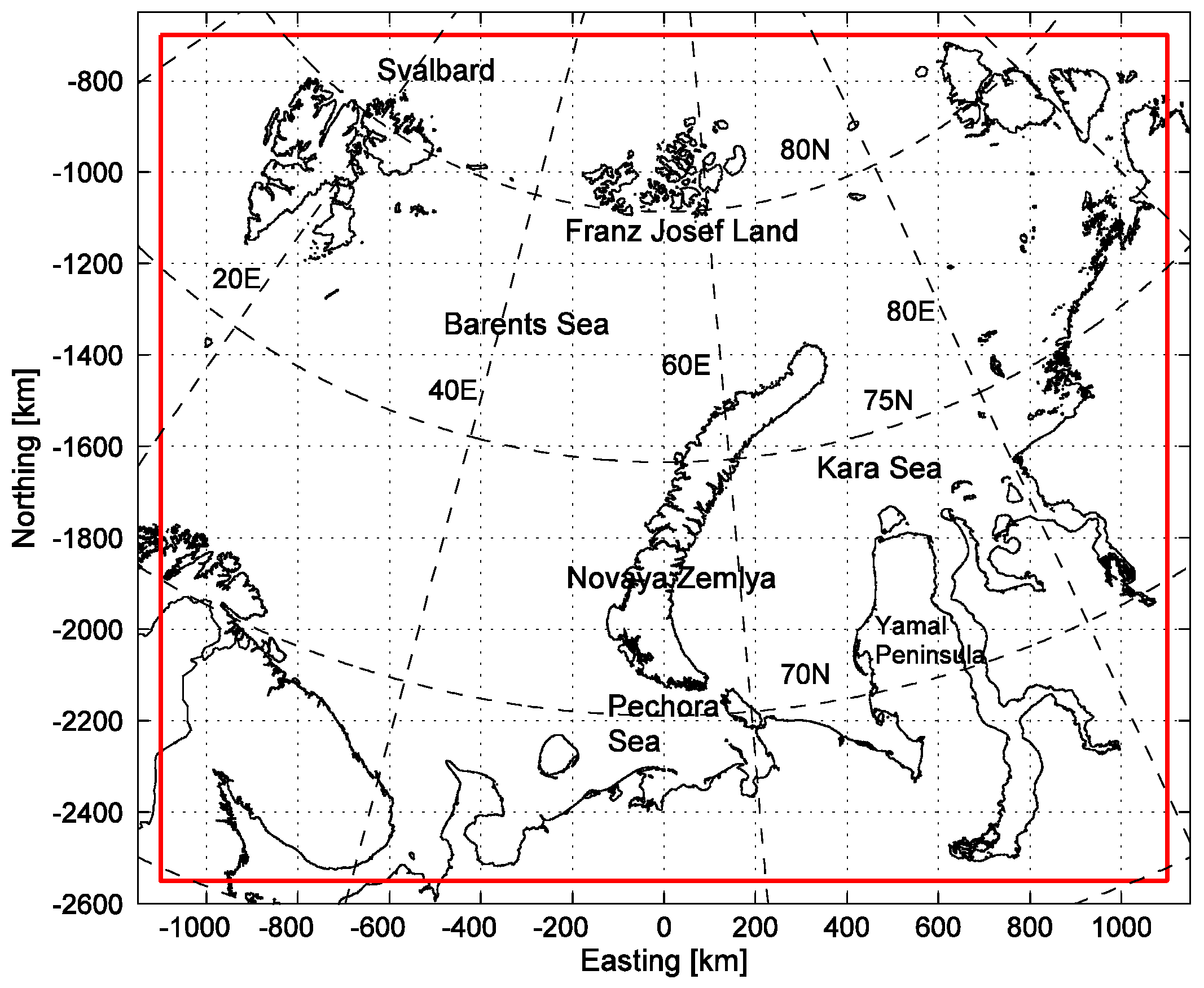
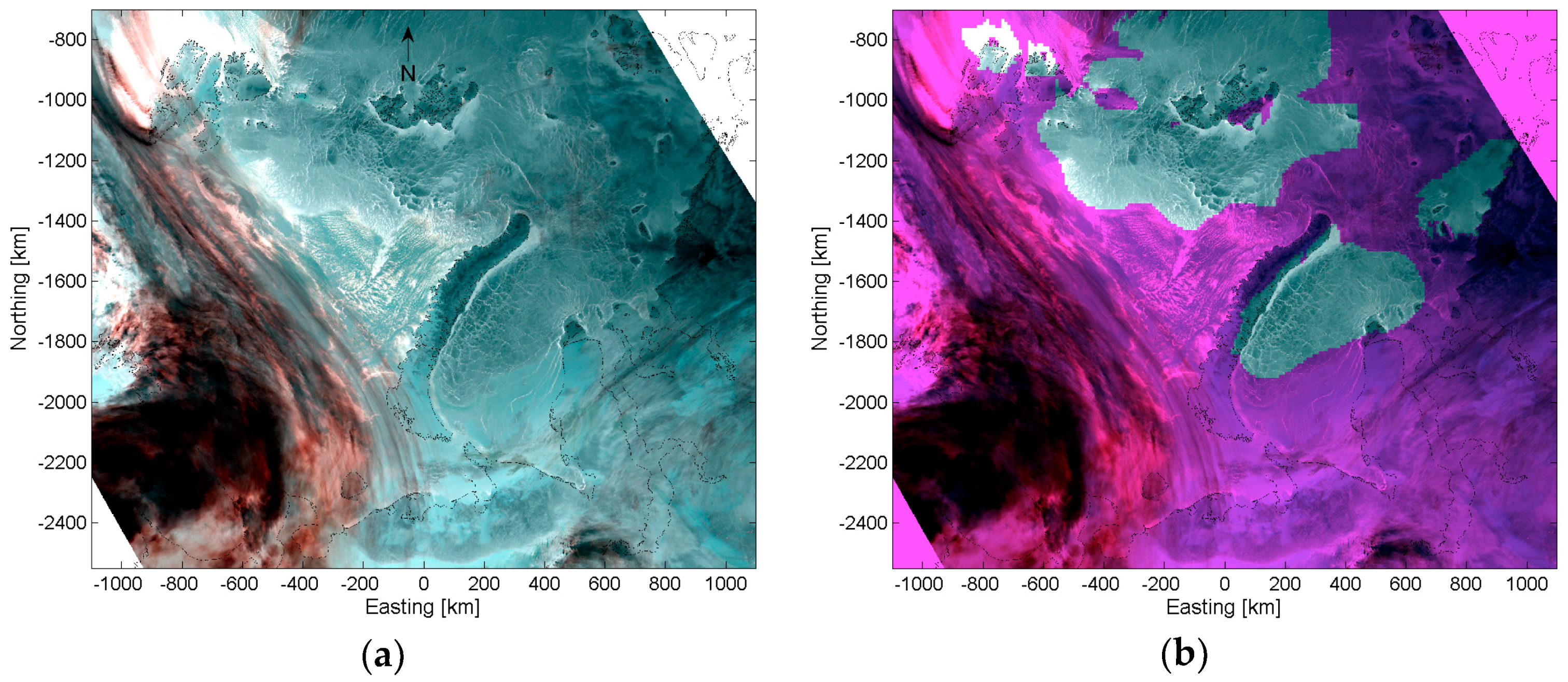
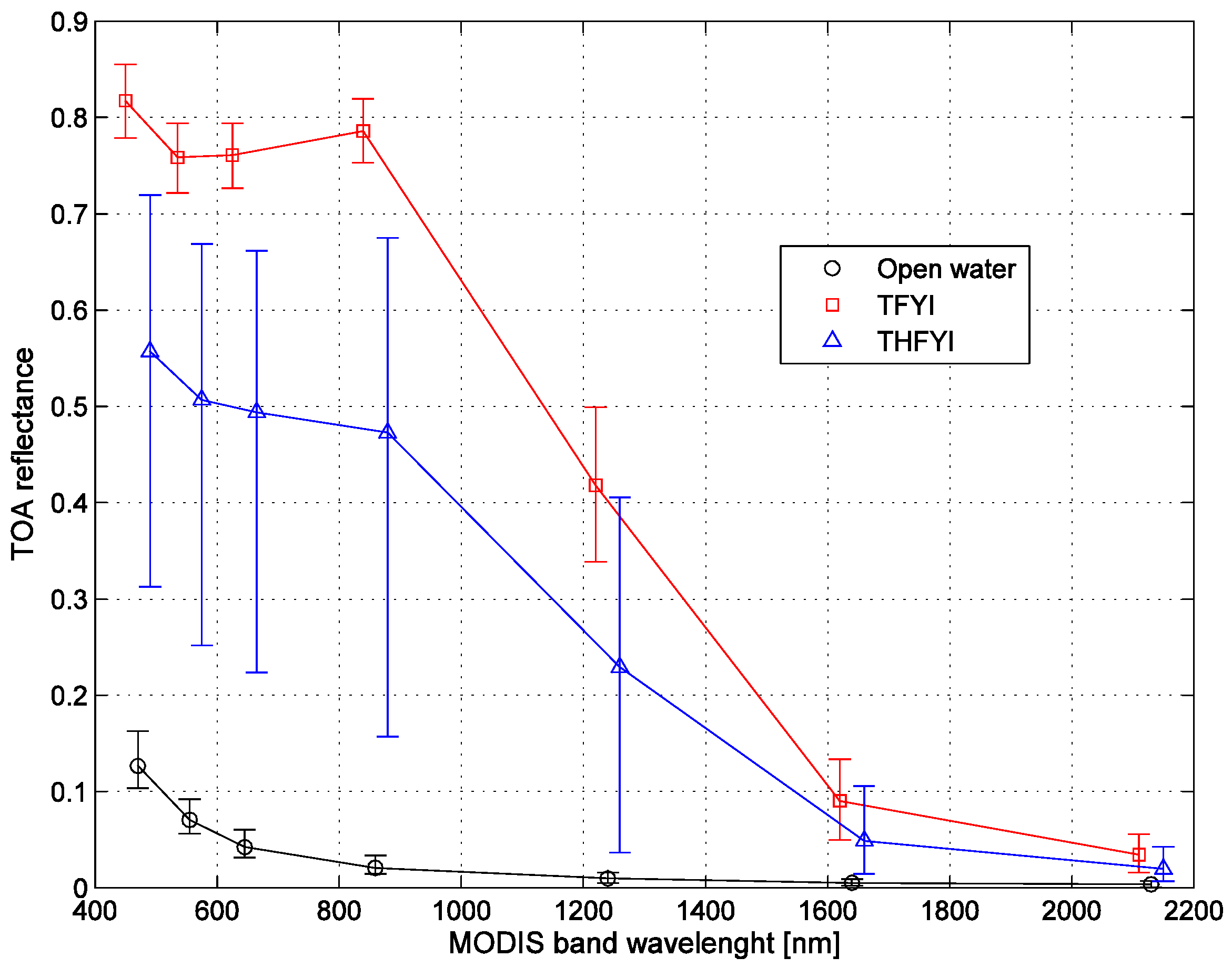
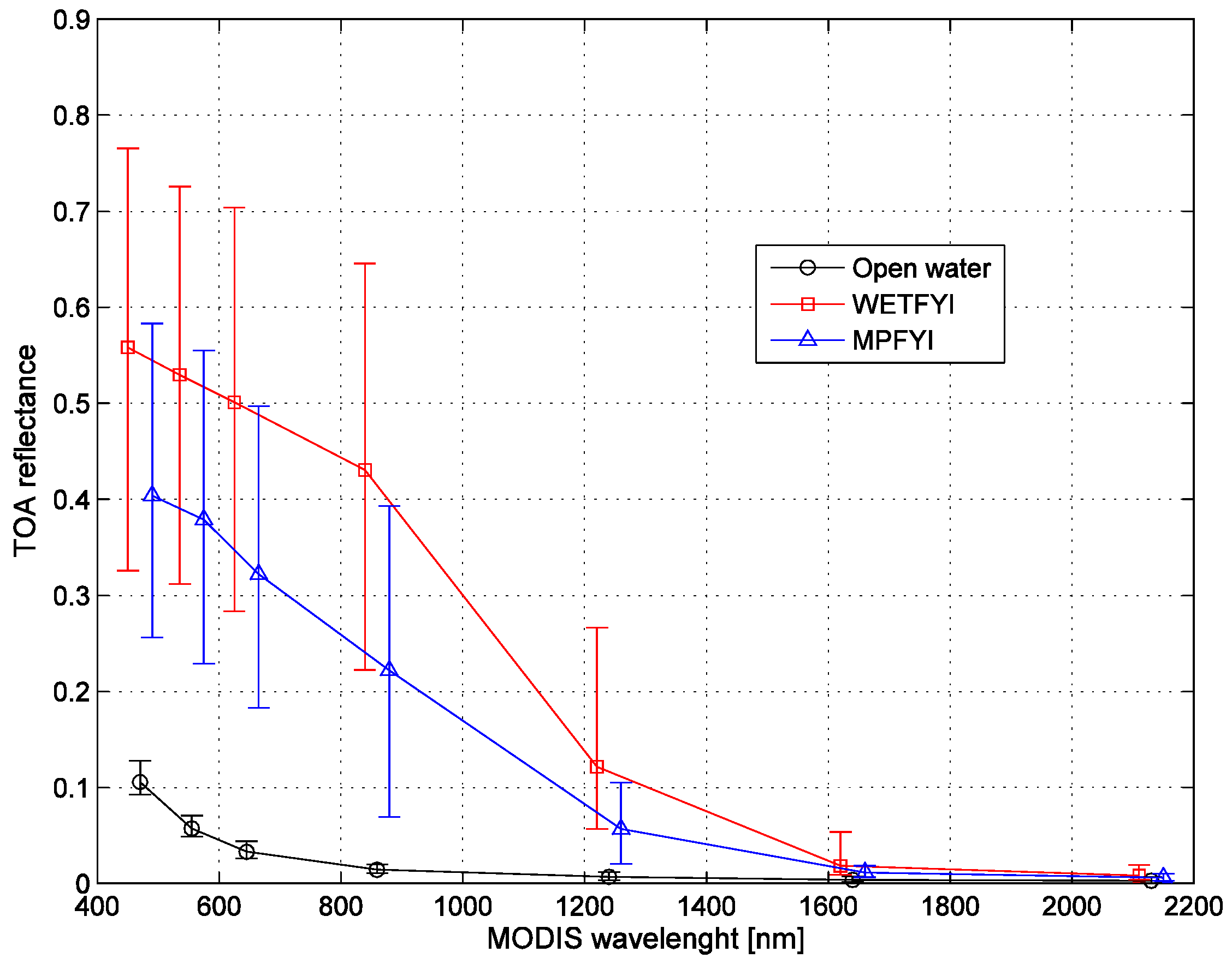
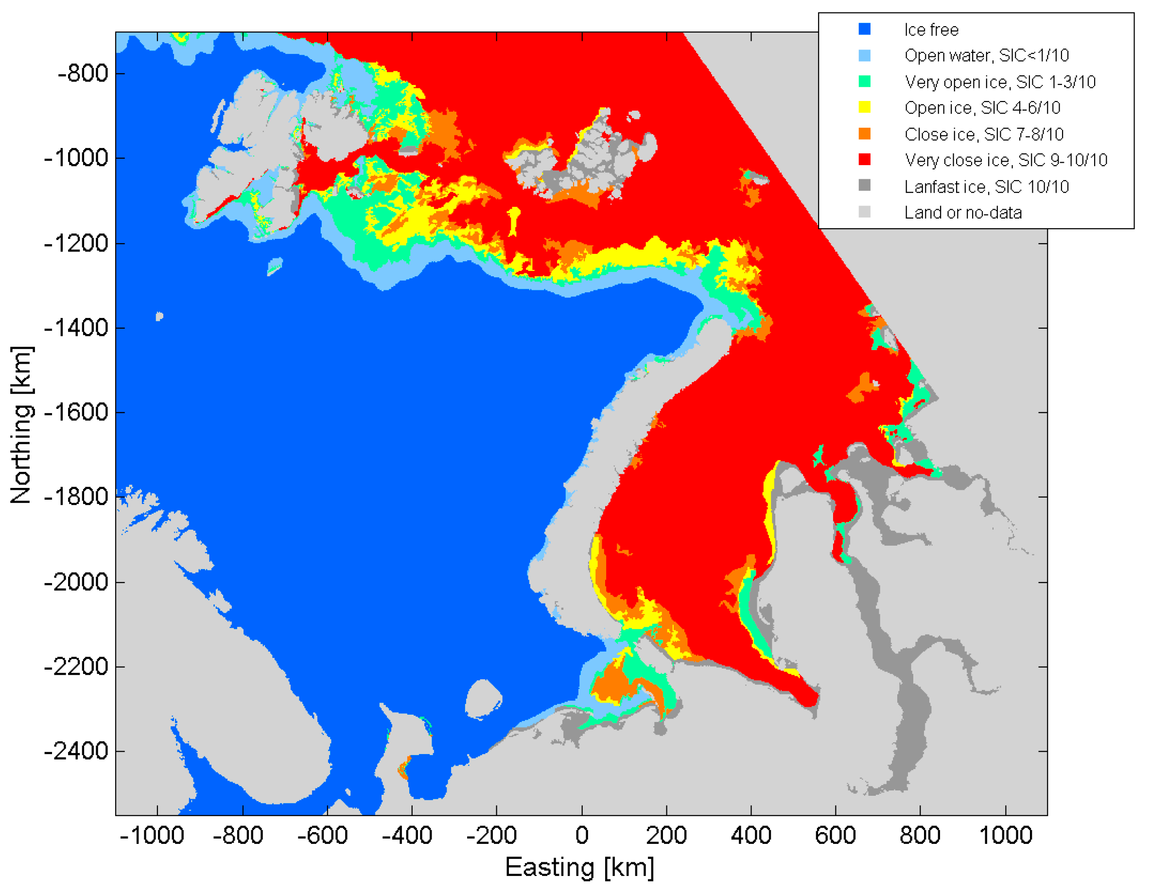
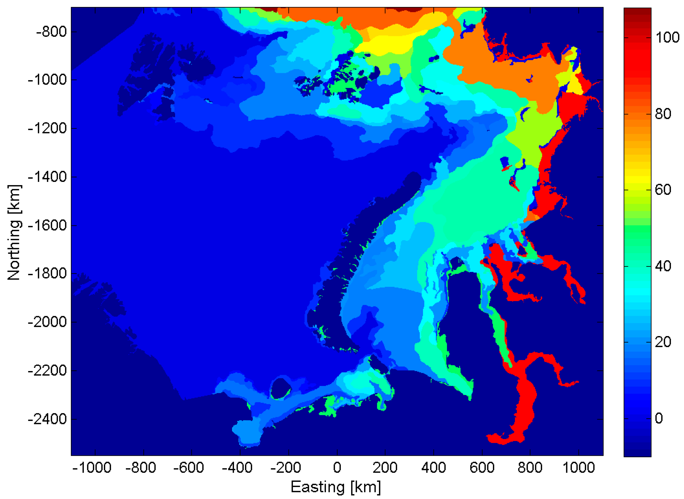
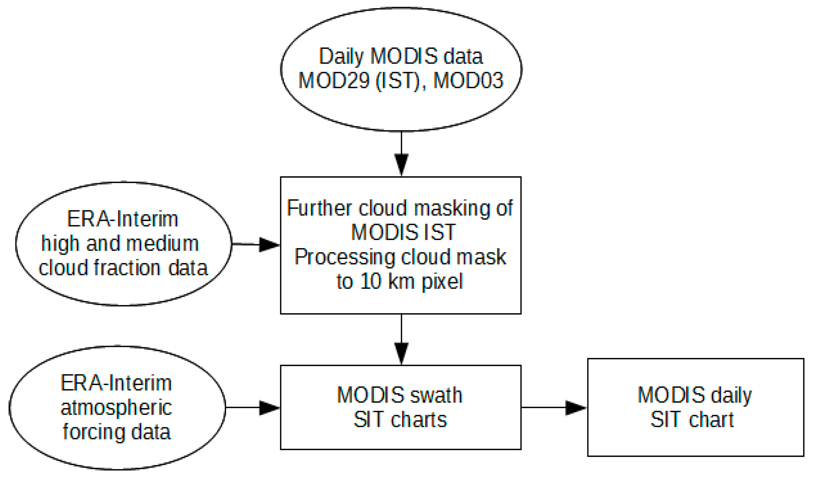
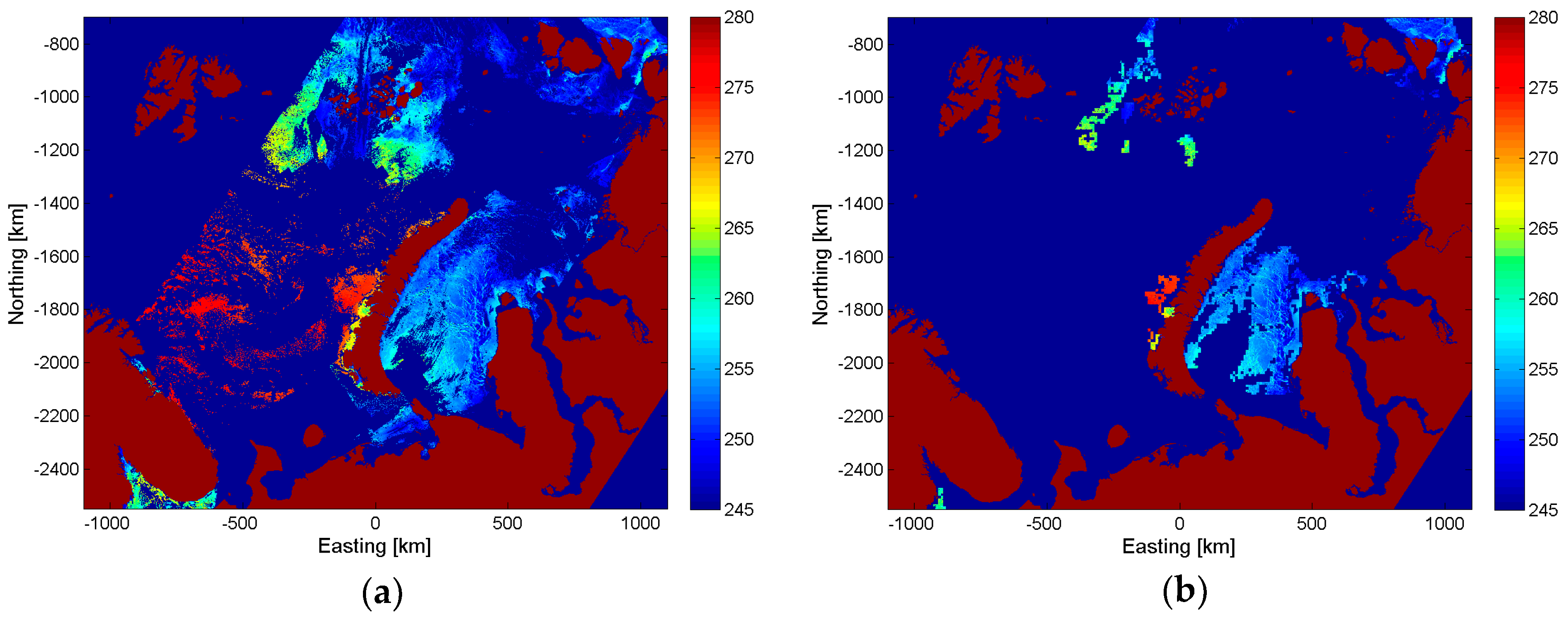
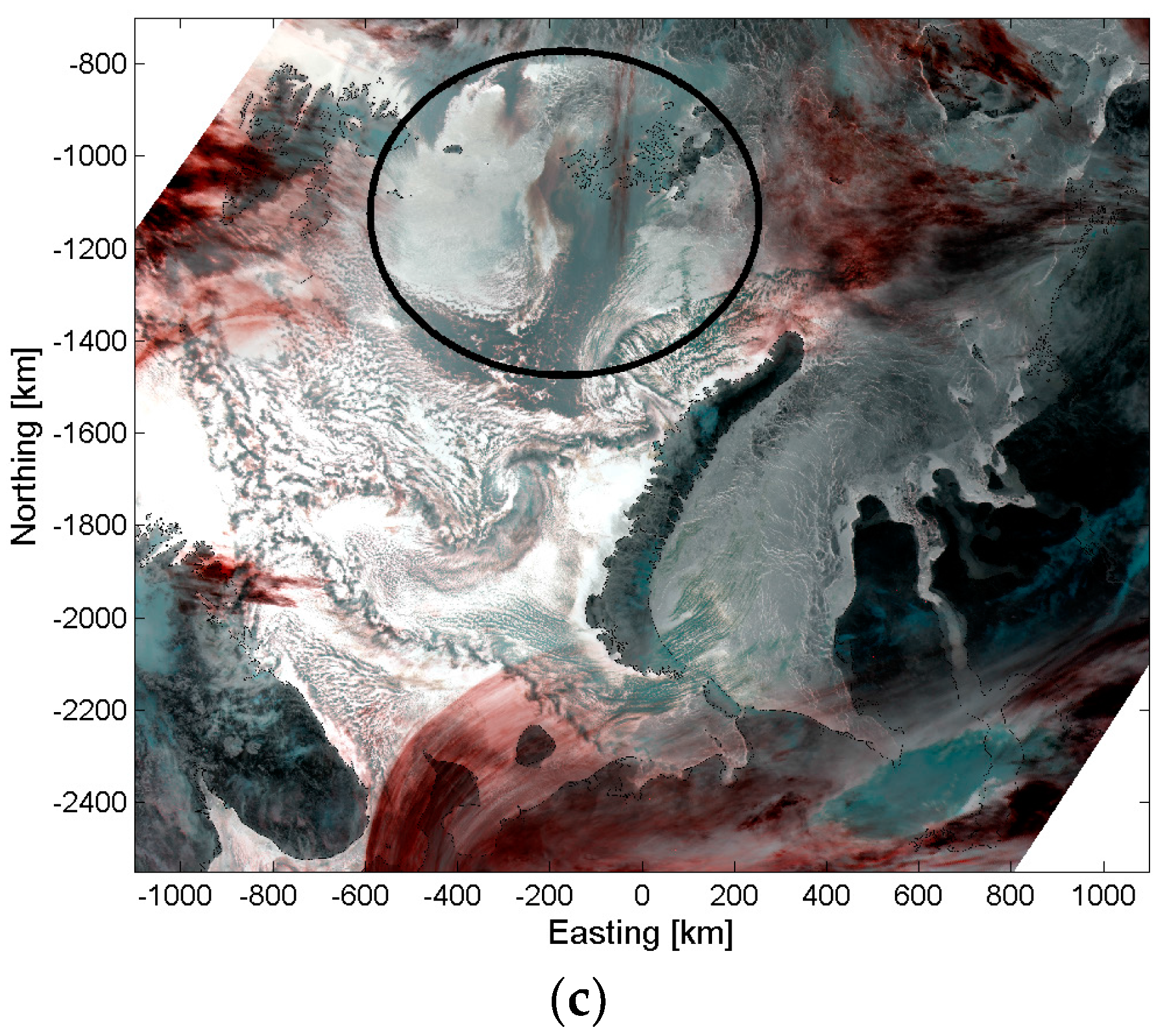
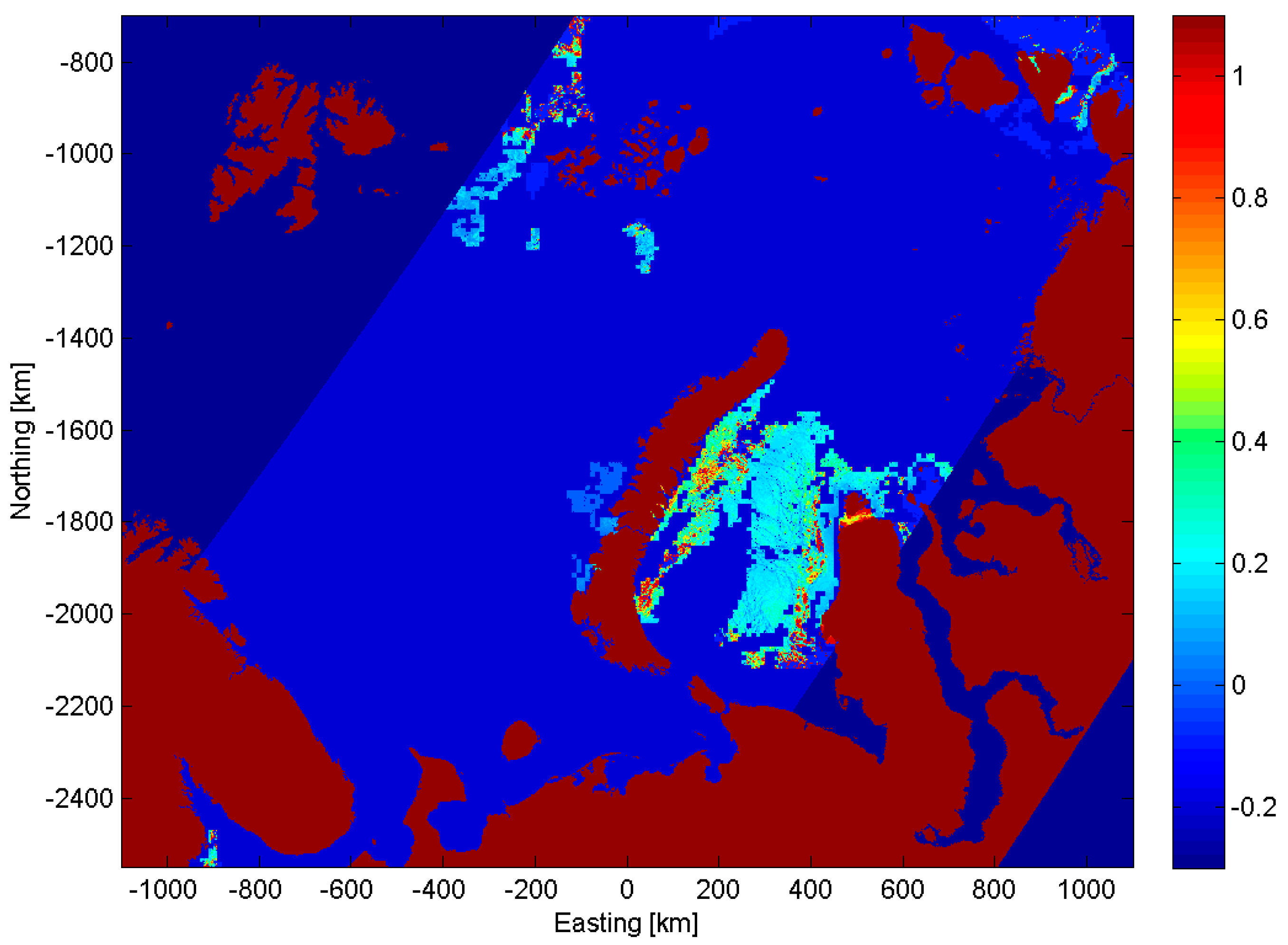
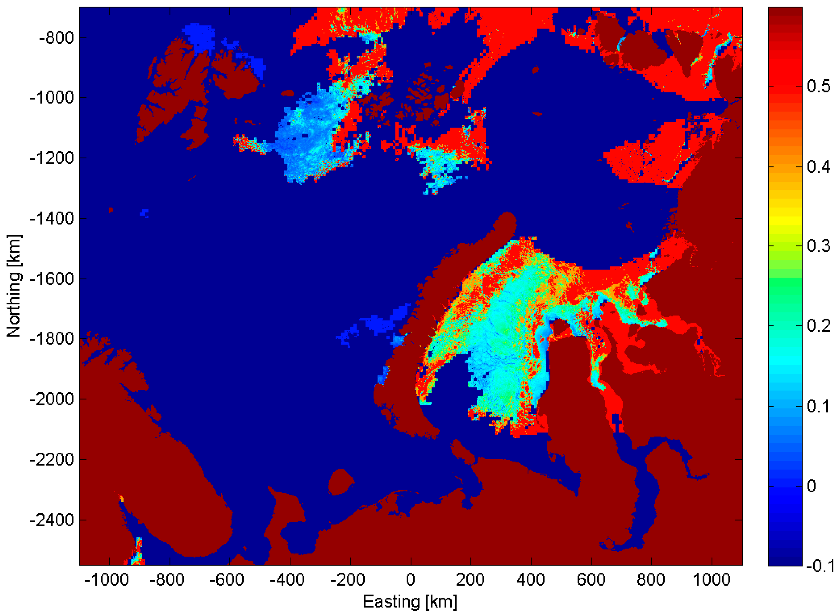
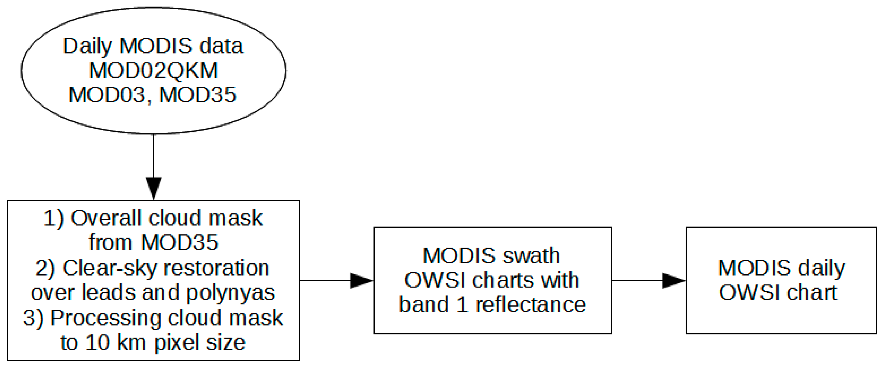
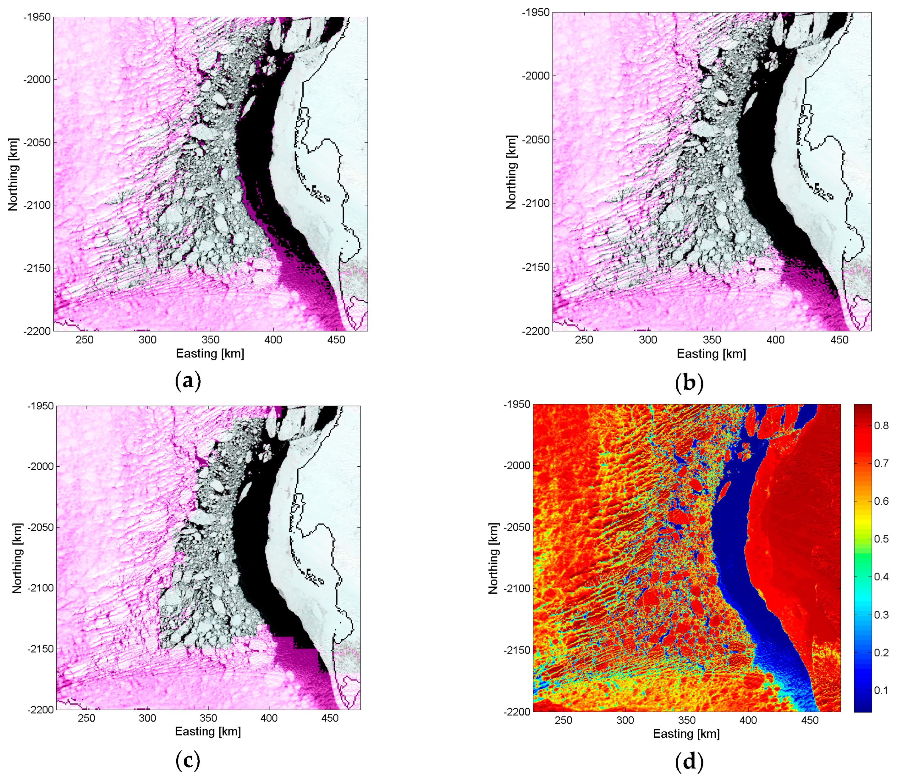
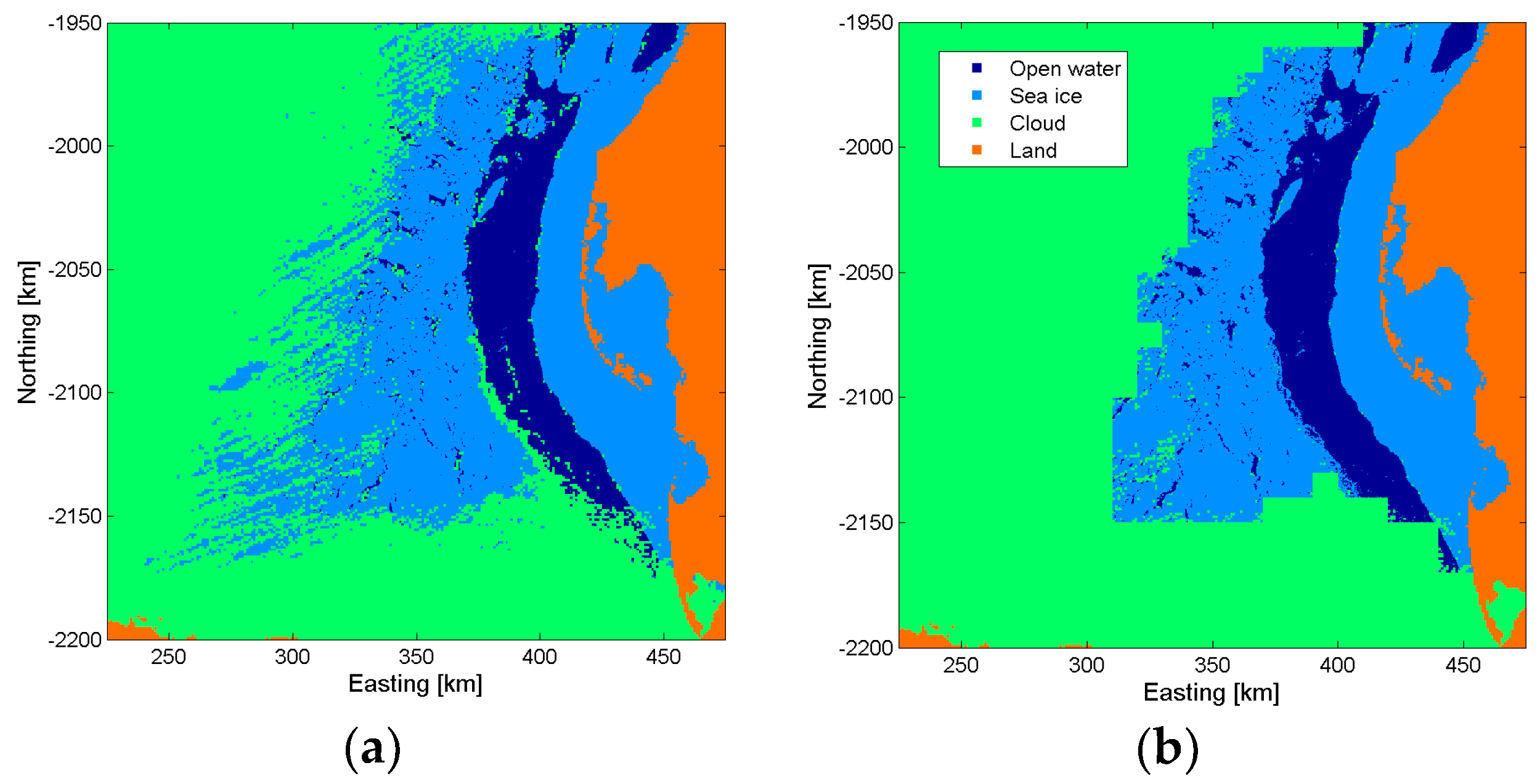
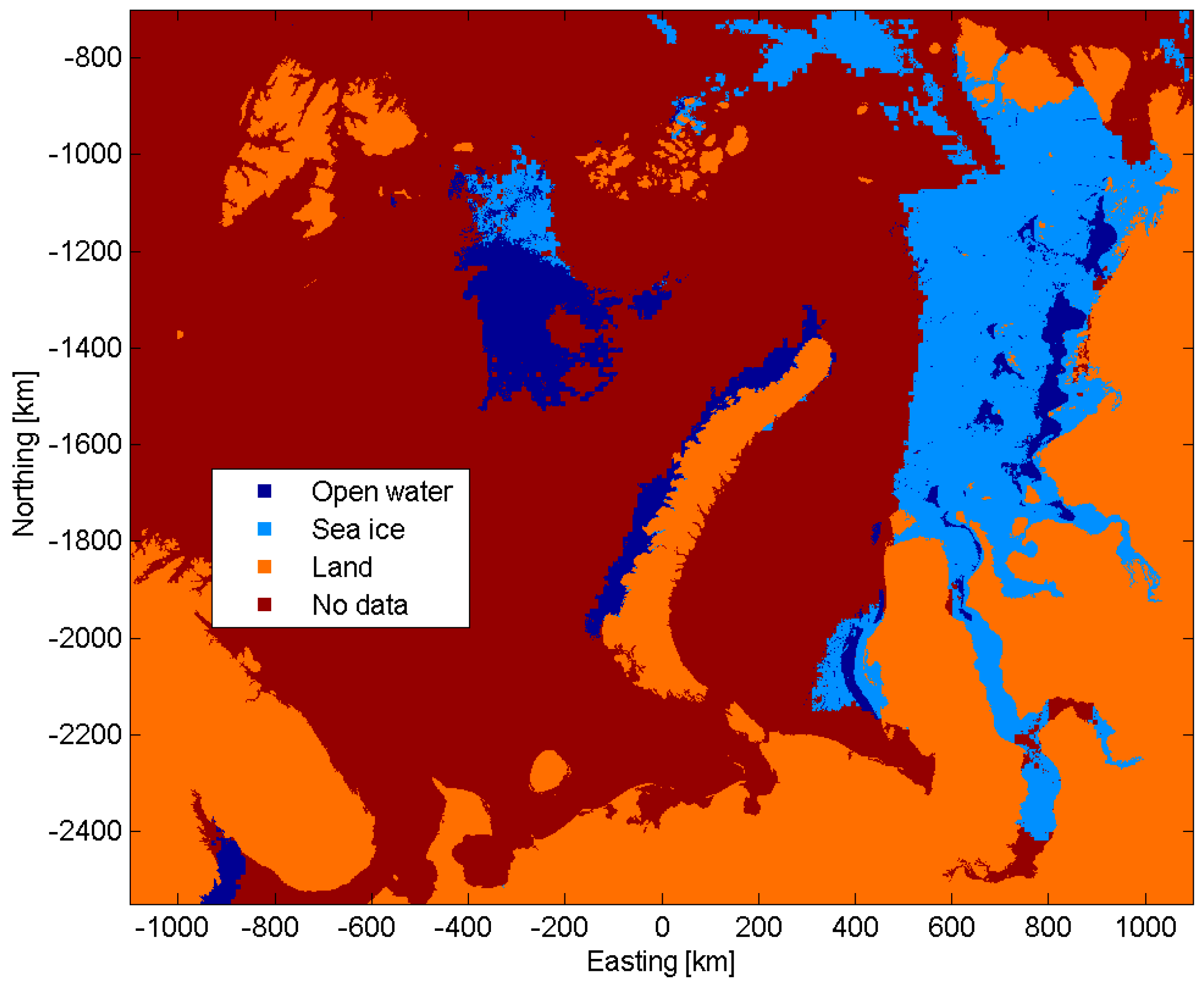
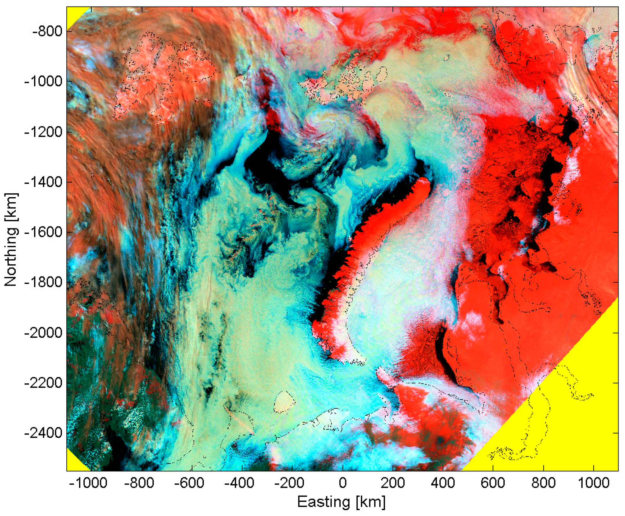
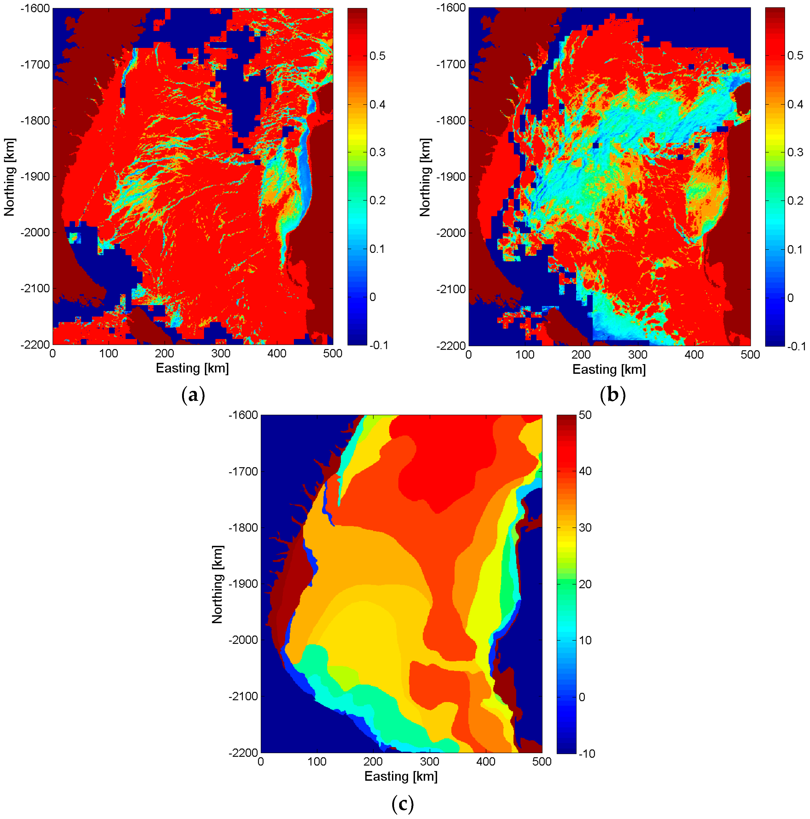
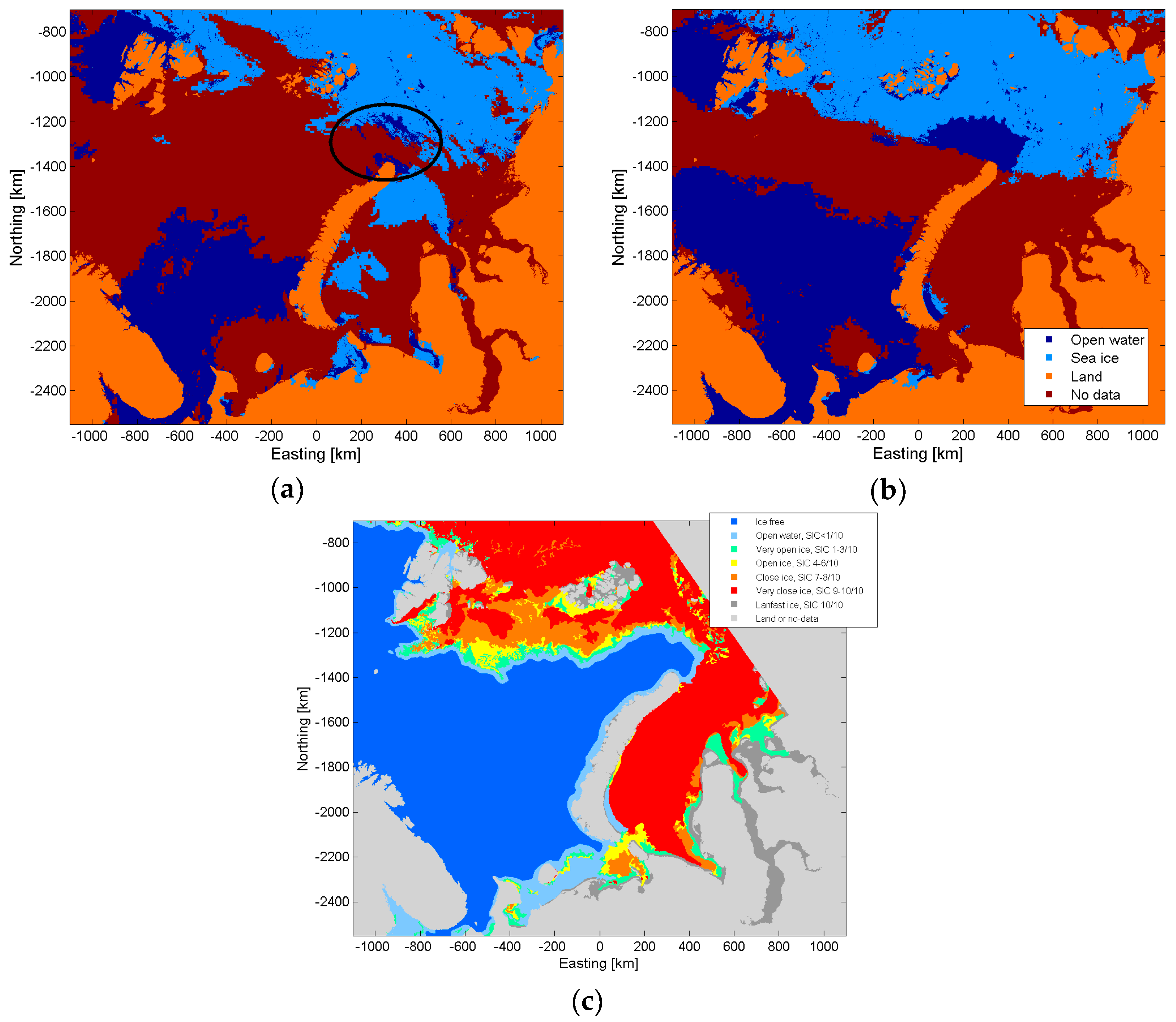
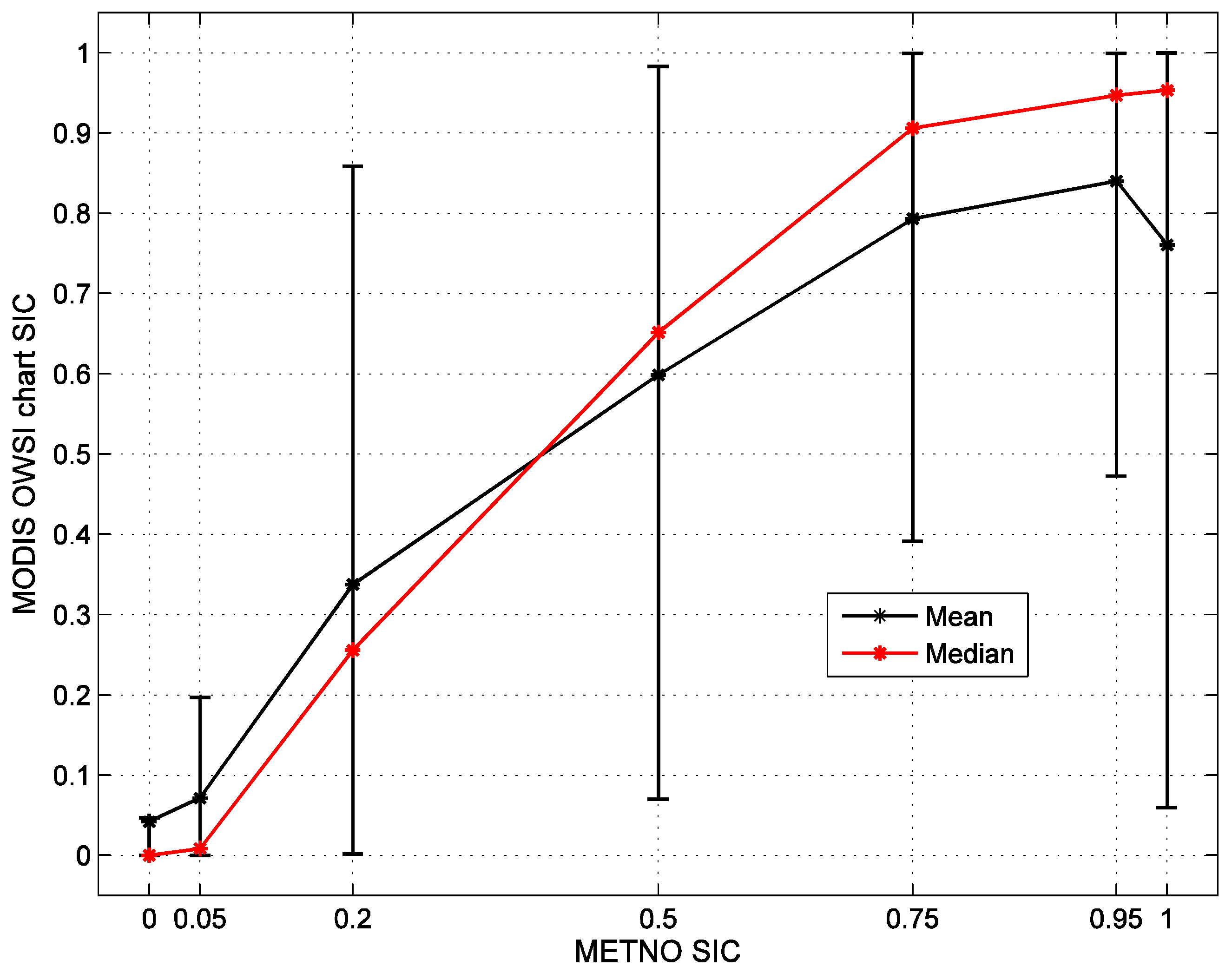
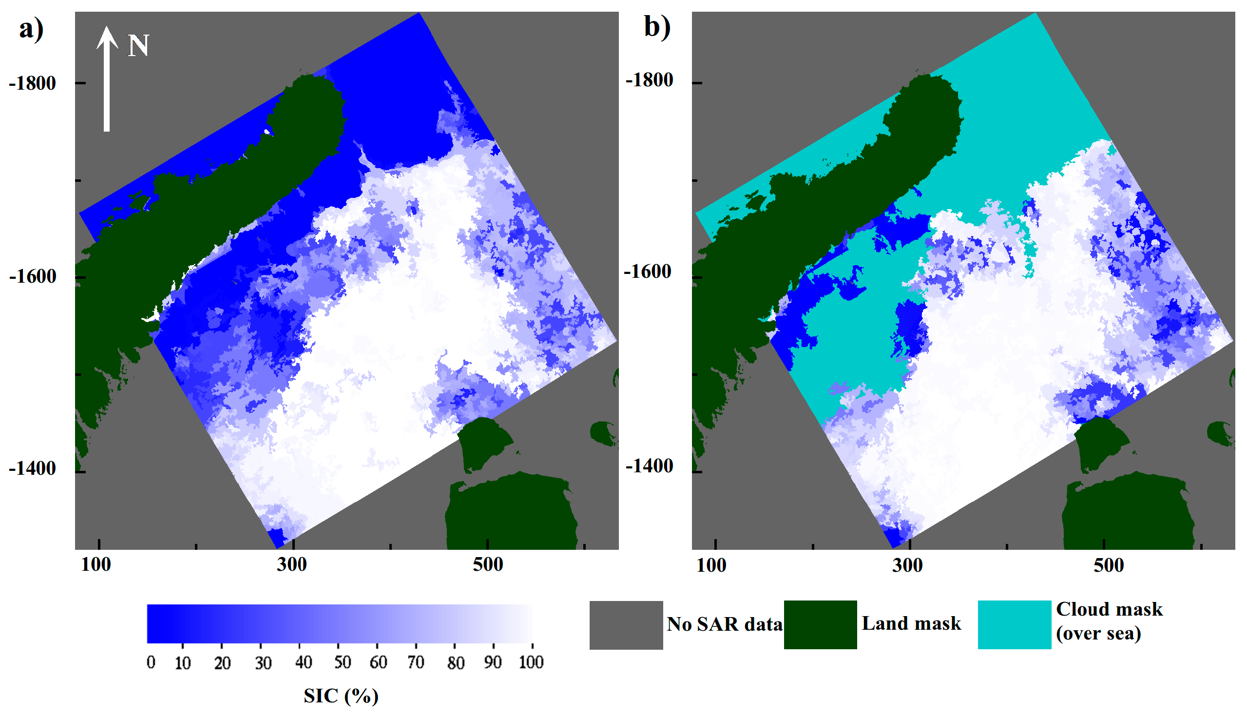
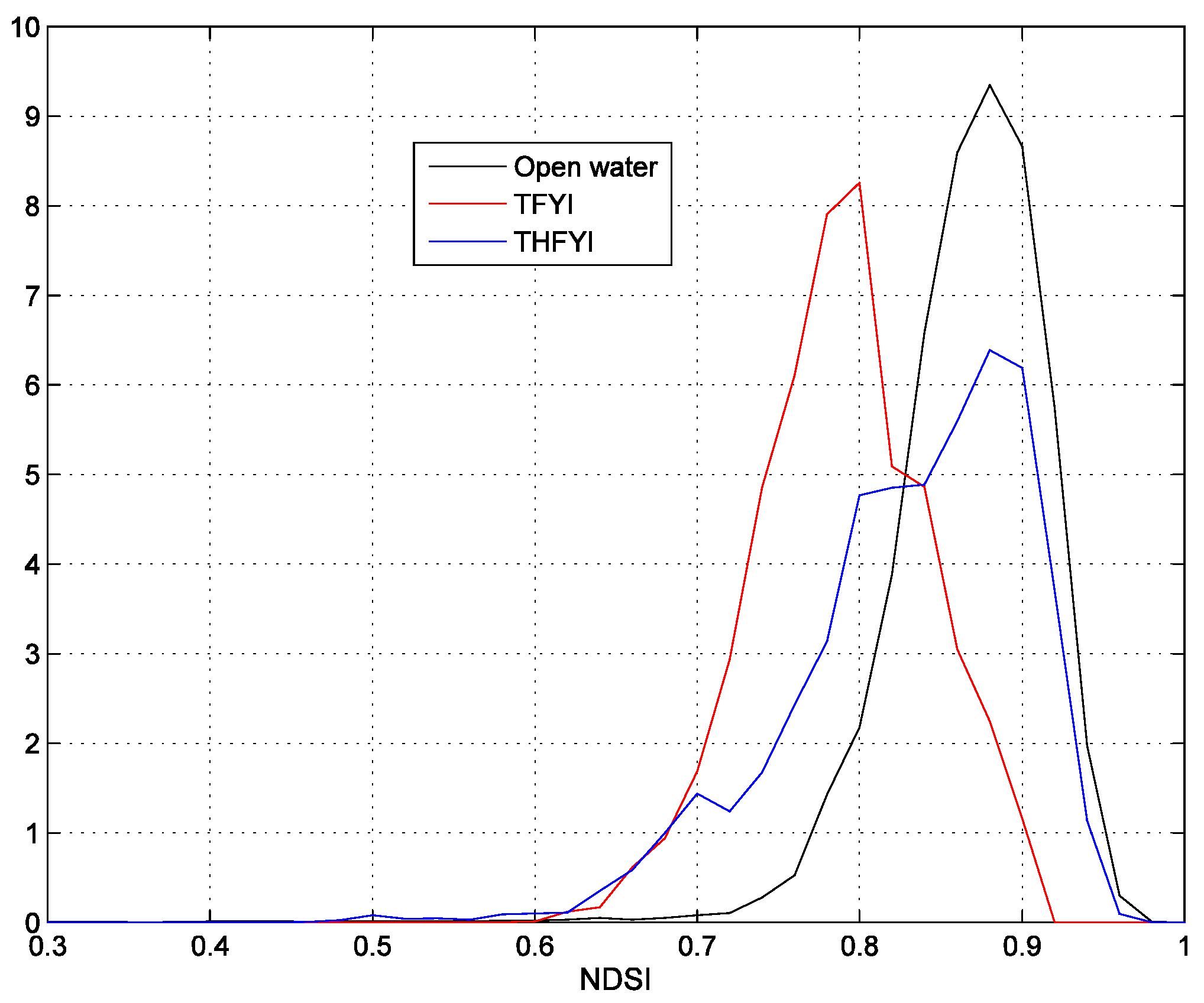