Intraspecific Differences in Spectral Reflectance Curves as Indicators of Reduced Vitality in High-Arctic Plants

 ,
,  , ,
, ,  ,
,  and
and
Abstract
1. Introduction
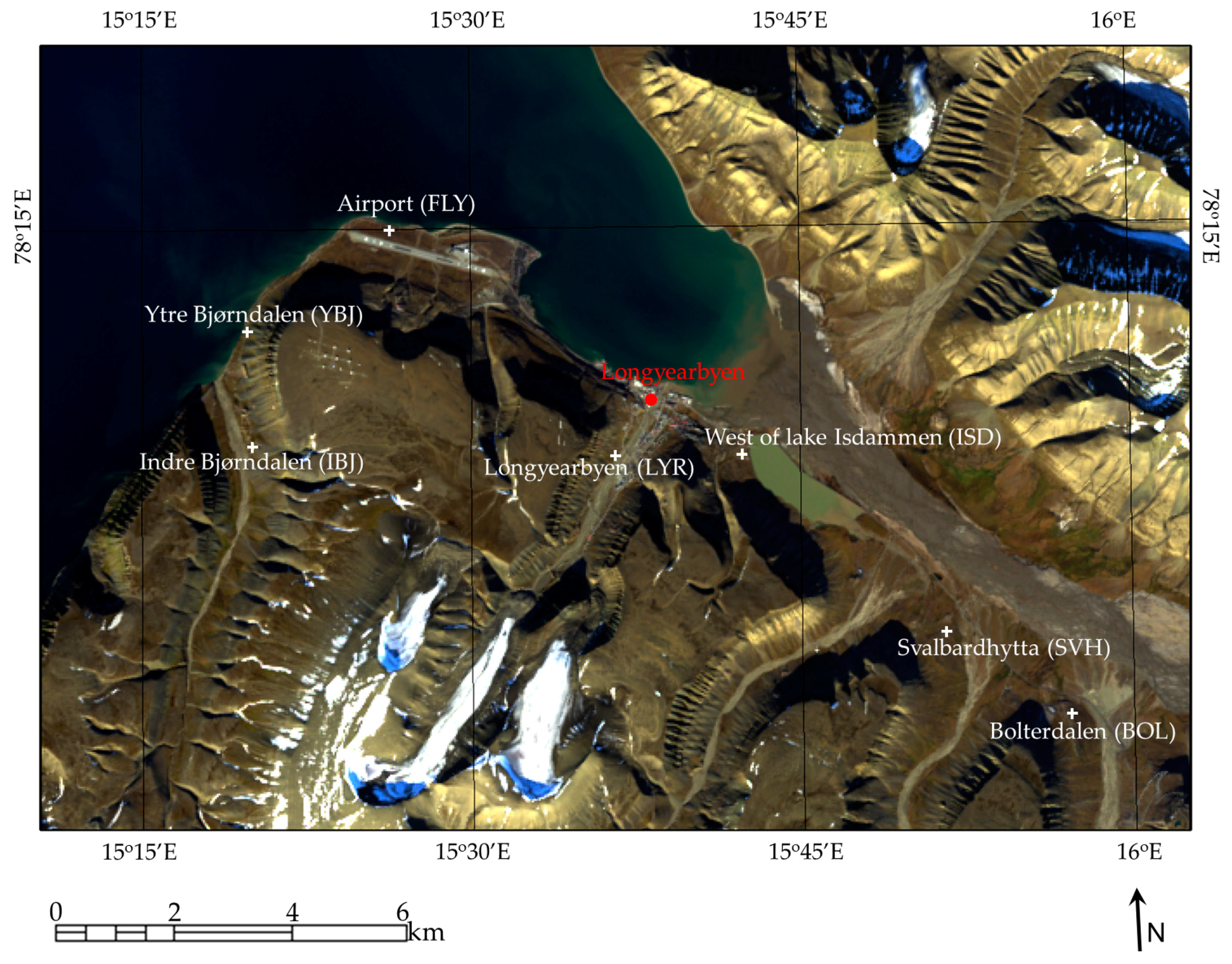
2. Study Area
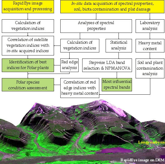
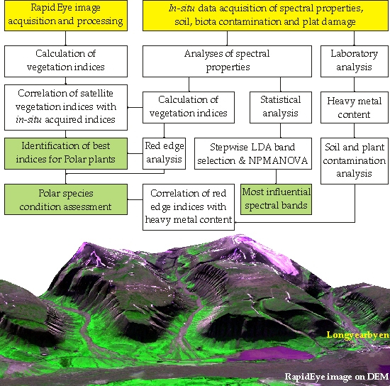
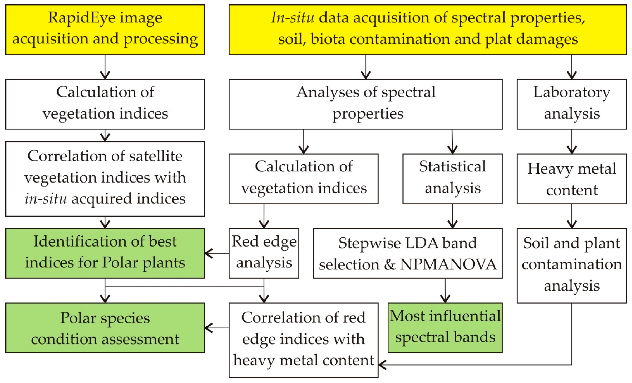
3. Materials and Methods
3.1. In-Situ Data Collection and Processing
3.2. Calculation of Vegetation Indices
3.3. Remotely Sensed Data from RapidEye
3.4. Statistical Analysis
4. Results
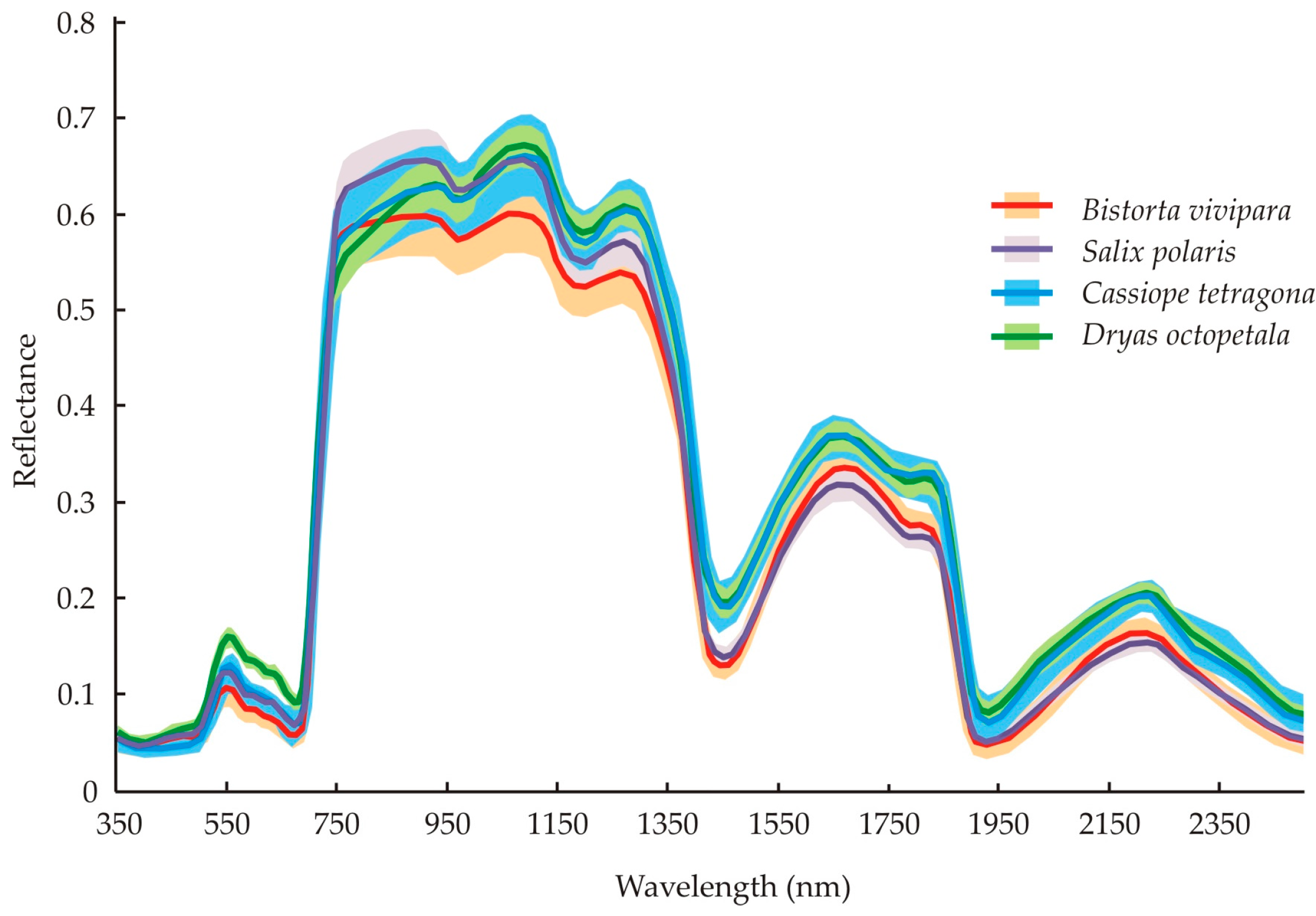
4.1. Differences between Species’
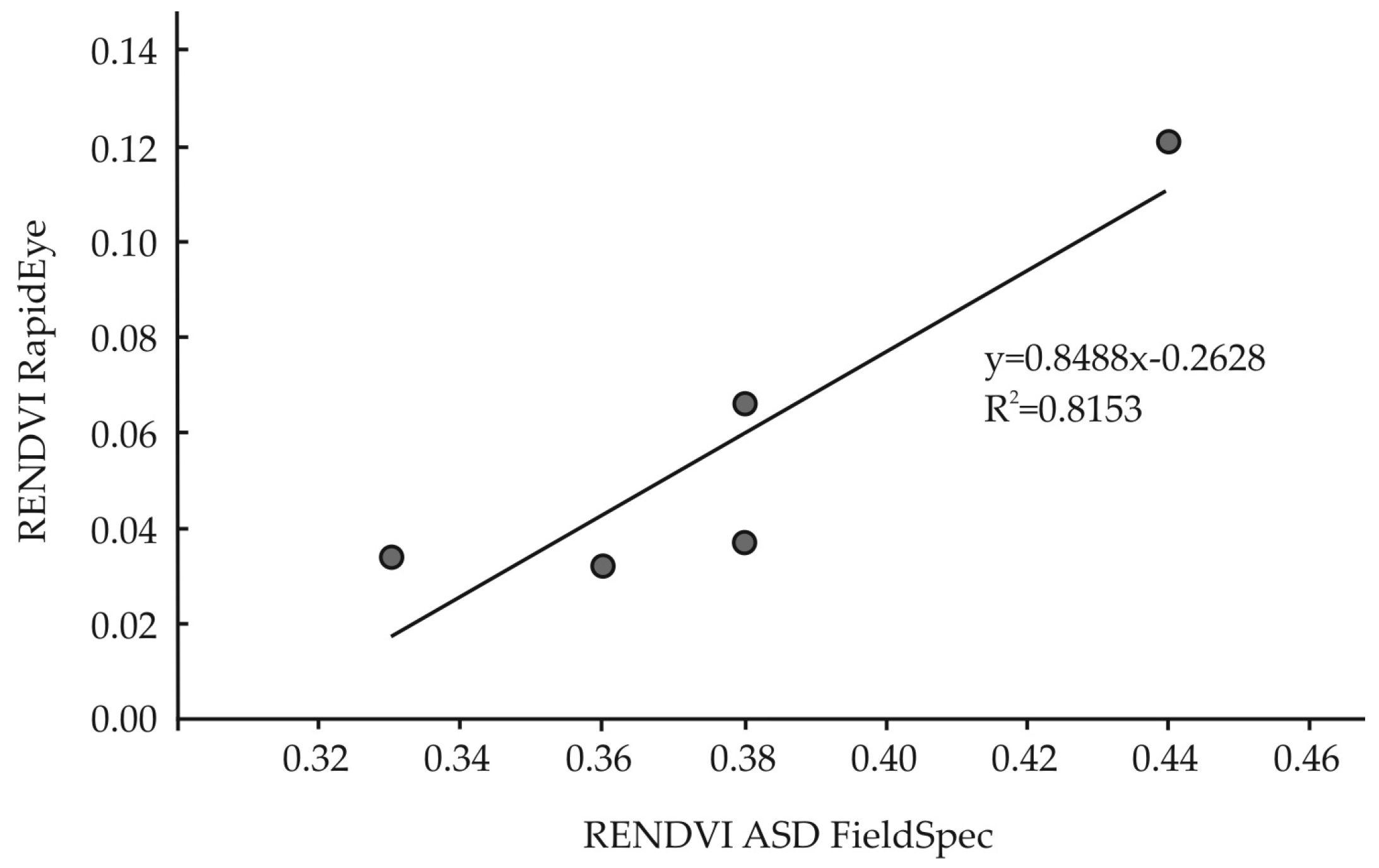
4.2. Plant Species Condition Assessment
5. Discussion
6. Conclusions
Acknowledgments
Author Contributions
Conflicts of Interest
References
- Jia, G.J.; Epstein, H.E.; Walker, D.A. Greening of arctic Alaska, 1981–2001. Geophys. Res. Lett. 2003, 30, 2067–2070. [Google Scholar] [CrossRef]
- Beck, P.S.A.; Goetz, S.J. Satellite observations of high northern latitude vegetation productivity changes between 1982 and 2008: Ecological variability and regional differences. Environ. Res. Lett. 2011, 6, 045501. [Google Scholar] [CrossRef]
- Xu, L.; Myneni, R.B.; Chapin, F.S., III; Callaghan, T.V.; Pinzon, J.E.; Tucker, C.J.; Zhu, Z.; Bi, J.; Ciais, P.; Tømmervik, H.; et al. Temperature and Vegetation Seasonality Diminishment over Northern Lands. Nat. Clim. Chang. 2013, 3, 581–586. [Google Scholar] [CrossRef]
- Beck, P.S.A.; Goetz, S.J.; Mack, M.C.; Alexander, H.D.; Jin, Y.; Randerson, J.T.; Loranty, M.M. The impacts and implications of an intensifying fire regime on Alaskan boreal forest composition and albedo. Glob. Chang. Biol. 2011, 17, 2853–2866. [Google Scholar] [CrossRef]
- McDowell, N.G.; Coops, N.C.; Beck, P.S.A.; Chambers, J.Q.; Gangodagamage, C.; Hicke, J.A.; Huang, C.; Kennedy, R.; Krofcheck, D.J.; Litvak, M.; et al. Global satellite monitoring of climate-induced vegetation disturbances. Trends Plant Sci. 2015, 20, 114–123. [Google Scholar] [CrossRef] [PubMed]
- Bjerke, J.W.; Treharne, R.; Vikhamar-Schuler, D.; Karlsen, S.R.; Ravolainen, V.; Bokhorst, S.; Phoenix, G.K.; Bochenek, Z.; Tømmervik, H. Understanding the drivers of extensive plant damage in boreal and Arctic ecosystems: Insights from field surveys in the aftermath of damage. Sci. Total Environ. 2017, 599–600, 1965–1976. [Google Scholar] [CrossRef] [PubMed]
- Bokhorst, S.F.; Bjerke, J.W.; Tømmervik, H.; Callaghan, T.V.; Phoenix, G.K. Winter warming events damage sub-Arctic vegetation: Consistent evidence from an experimental manipulation and a natural event. J. Ecol. 2009, 97, 1408–1415. [Google Scholar] [CrossRef]
- Bjerke, J.W.; Karlsen, S.R.; Høgda, K.A.; Malnes, E.; Jepsen, J.U.; Lovibond, S.; Vikhamar Schuler, D.; Tømmervik, H. Record-low primary productivity and high plant damage in the Nordic Arctic Region in 2012 caused by multiple weather events and pest outbreaks. Environ. Res. Lett. 2014, 9, 084006. [Google Scholar] [CrossRef]
- Snow, Water, Ice and Permafrost in the Arctic (SWIPA): Climate Change and the Cryosphere; Arctic Monitoring and Assessment Programme (AMAP): Oslo, Norway, 2011.
- Tømmervik, H. Vegetation damage studies in the Jarfjordfjell area, Northern Norway, by use of airborne CASI spatial mode data. Remote Sens. Rev. 2000, 18, 19–51. [Google Scholar] [CrossRef]
- Tømmervik, H.; Høgda, K.A.; Solheim, I. Monitoring vegetation changes in Pasvik (Norway) and Pechenga in Kola Peninsula (Russia) using multi-temporal Landsat MSS/TM data. Remote Sens. Environ. 2003, 85, 370–388. [Google Scholar] [CrossRef]
- Askaer, L.; Schmidt, L.B.; Elberling, B.; Asmund, G.; Jonsdottir, I.S. Environmental impact on an Arctic Soil–Plant System resulting from metals released from coal mine waste in Svalbard (78°N). Water Air Soil Pollut. 2008, 195, 99–114. [Google Scholar] [CrossRef]
- Thenkabail, P.S.; Smith, R.B.; De Pauw, E. Hyperspectral vegetation indices and their relationships with agricultural crop characteristics. Remote Sens. Environ. 2000, 71, 158–182. [Google Scholar] [CrossRef]
- Kycko, M.; Zagajewski, B.; Kozlowska, A. Variability in spectral characteristics of trampled high-mountain grasslands. Misc. Geogr. 2014, 18, 10–14. [Google Scholar] [CrossRef]
- Jarocińska, A.M.; Kacprzyk, M.; Marcinkowska-Ochtyra, A.; Ochtyra, A.; Zagajewski, B.; Meuleman, K. The application of APEX images in the assessment of the state of non-forest vegetation in the Karkonosze Mountains. Misc. Geogr. 2016, 20, 21–27. [Google Scholar] [CrossRef]
- Solheim, I.; Engelsen, O.; Hosgood, B.; Andreoli, G. Measurement and Modeling of the Spectral and Directional Reflection Properties of Lichen and Moss Canopies. Remote Sens. Environ. 2000, 72, 78–94. [Google Scholar] [CrossRef]
- Rees, W.G.; Tutubalina, O.V.; Golubeva, E.I. Reflectance spectra of subarctic lichens between 400 and 2400 nm. Remote Sens. Environ. 2004, 90, 281–292. [Google Scholar] [CrossRef]
- Vierling, L.A.; Deering, D.W.; Eck, T.F. Differences in arctic tundra vegetation type and phenology as seen using bidirectional radiometry in the early growing season. Remote Sens. Environ. 1997, 60, 71–82. [Google Scholar] [CrossRef]
- Buchhorn, M.; Walker, D.A.; Heim, B.; Raynolds, M.K.; Epstein, H.E.; Schwider, M. Ground-Based Hyperspectral Characterization of Alaska tundra vegetation along environmental gradients. Remote Sens. Environ. 2013, 5, 3971–4005. [Google Scholar] [CrossRef]
- Adam, E.; Mutanga, O. Spectral discrimination of papyrus vegetation (Cyperus papyrus L.) in swamp wetlands using field spectrometry. ISPRS J. Photogramm. Remote Sens. 2009, 64, 612–620. [Google Scholar] [CrossRef]
- Campioli, M.; Street, L.E.; Michelsen, A.; Shaver, G.R.; Maere, T.; Samson, R.; Lemeru, R. Determination of leaf area index, total foliar N, and normalized difference vegetation index for Arctic ecosystems dominated by Cassiope tetragona. Arct. Antarct. Alp. Res. 2009, 4, 426–433. [Google Scholar] [CrossRef]
- Zagajewski, B. Assessment of neural networks and Imaging Spectroscopy for vegetation classification of the High Tatras. Teledetekcja Środowiska 2011, 43, 113. [Google Scholar]
- Jelének, J.; Kupková, L.; Zagajewski, B.; Březina, S.; Ochytra, A.; Marcinkowska, A. Laboratory and image spectroscopy for evaluating the biophysical state of meadow vegetation in the Krkonoše National Park. Misc. Geogr. 2014, 18, 15–22. [Google Scholar] [CrossRef]
- Marcinkowska, A.; Zagajewski, B.; Ochtyra, A.; Jarocińska, A.; Raczko, E.; Kupková, L.; Stych, P.; Meuleman, K. Mapping vegetation communities of the Karkonosze National Park using APEX hyperspectral data and Support Vector Machines. Misc. Geogr. 2014, 18, 23–29. [Google Scholar] [CrossRef]
- Walker, D.A.; Raynolds, M.K.; Daniëls, F.J.A.; Einarsson, E.; Elvebakk, A.; Gould, W.A.; Katenin, A.E.; Kholod, S.S.; Markon, C.J.; Melnikov, E.S.; et al. The Circumpolar Arctic Vegetation Map. J. Veg. Sci. 2005, 16, 267–282. [Google Scholar] [CrossRef]
- Epstein, H.E.; Raynolds, M.K.; Walker, D.A.; Bhatt, U.S.; Tucker, C.J.; Pinzon, J.E. Dynamics of aboveground phytomass of the circumpolar Arctic tundra during the past three decades. Environ. Res. Lett. 2012, 7, 015506. [Google Scholar] [CrossRef]
- Johansen, B.E.; Karlsen, S.R.; Tømmervik, H. Vegetation mapping of Svalbard utilising Landsat TM/ETM+ data. Polar Rec. 2012, 48, 47–63. [Google Scholar] [CrossRef]
- Johansen, B.E.; Tømmervik, H. The relationship between phytomass, NDVI and vegetation communities on Svalbard. Int. J. Appl. Earth Obs. Geoinf. 2013, 27, 20–30. [Google Scholar] [CrossRef]
- Tømmervik, H.; Karlsen, S.R.; Nilsen, L.; Johansen, B.; Storvold, R.; Zmarz, A.; Beck, P.S.; Johansen, K.S.; Høgda, K.A.; Goetz, S.; et al. Use of unmanned aircraft systems (UAS) in a multiscale vegetation index study of Arctic plant communities in Adventdalen on Svalbard. EARSeL eProceed. 2014, 13, 47–52. [Google Scholar] [CrossRef]
- Store Norske Spitsbergen Kullkompani AS. Available online: https://snl.no/Store_Norske_Spitsbergen_Kulkompani_AS (accessed on 30 December 2016).
- Kłos, A.; Bochenek, Z.; Bjerke, J.W.; Zagajewski, B.; Ziółkowski, D.; Ziembik, Z.; Rajfur, M.; Dołhańczuk-Śródka, A.; Tømmervik, H.; Krems, P.; et al. The use of mosses in biomonitoring of selected areas in Poland and Spitsbergen in the years from 1975 to 2014. Ecol. Chem. Engine 2015, S22, 201–218. [Google Scholar] [CrossRef]
- Van der Wal, R.; Stien, A. High-arctic plants like it hot: A long-term investigation of between-year variability in plant biomass. Ecology 2014, 95, 3414–3427. [Google Scholar] [CrossRef]
- Hansen, B.B.; Isaksen, K.; Benestad, R.E.; Kohler, J.; Pedersen, Å.Ø.; Loe, L.E.; Coulson, S.J.; Larsen, J.O.; Varpe, Ø. Warmer and wetter winters: Characteristics and implications of an extreme weather event in the High Arctic. Environ. Res. Lett. 2014, 9, 114021. [Google Scholar] [CrossRef]
- Aarrestad, P.A.; Bakkestuen, V.; Hassel, K.; Stabbetorp, O.E.; Wilmann, B. Establishment of Monitoring Sitres for Ground Vegetation in Endalen, Svalbard 2009; NINA Report 579; Norsk Institutt for Naturforskning: Trondheim, Norway, 2010; pp. 1–62. [Google Scholar]
- Hultén, E.; Fries, M. Atlas of North European Vascular Plants: North of the Tropic of Cancer; Koeltz Scientific Books: Königstein, Germany, 1986. [Google Scholar]
- Mierczyk, M.; Zagajewski, B.; Jarocińska, A.; Knapik, R. Assessment of Imaging Spectroscopy for rock identification in the Karkonosze Mountains, Poland. Misc. Geogr. 2016, 20, 34–40. [Google Scholar] [CrossRef]
- Lichtenthaler, H.K.; Buschmann, C.; Rinderle, U.; Schmuck, G. Application of chlorophyll fluorescence in ecophysiology. Radiat. Environ. Biophys. 1986, 25, 297–308. [Google Scholar] [CrossRef] [PubMed]
- Clark, M.; Roberts, D.; Clark, D. Hyperspectral discrimination of tropical rain forest tree species at leaf to crown scales. Remote Sens. Environ. 2005, 96, 375–398. [Google Scholar] [CrossRef]
- Anderson, M.J. A new method for non-parametric multivariate analysis of variance. Austral Ecol. 2001, 26, 32–46. [Google Scholar] [CrossRef]
- Kłos, A.; Ziembik, Z.; Rajfur, M.; Dołhańczuk-Śródka, A.; Bochenek, Z.; Bjerke, J.W.; Tømmervik, H.; Zagajewski, B.; Ziółkowski, D.; Jerz, D.; et al. The Origin of Heavy Metals and Radionuclides Accumulated in the Soil and Biota Samples Collected in Svalbard, Near Longyearbyen. Ecol. Chem. Eng. S 2017, 24, 223–238. [Google Scholar] [CrossRef]
- Kupková, L.; Červená, L.; Suchá, R.; Jakešová, L.; Zagajewski, B.; Březina, S.; Albrechtová, J. Classification of Tundra Vegetation in the Krkonoše Mts. National Park Using APEX, AISA Dual and Sentinel-2A Data. Eur. J. Remote Sens. 2017, 50, 29–46. [Google Scholar] [CrossRef]
- Kycko, M.; Zagajewski, B.; Zwijacz-Kozica, M.; Cierniewski, J.; Romanowska, E.; Orłowska, K.; Ochtyra, A.; Jarocińska, A. Assessment of Hyperspectral Remote Sensing for Analyzing the Impact of Human Trampling on Alpine Swards. Mt. Res. Dev. 2017, 37, 66–74. [Google Scholar] [CrossRef]
- Marcinkowska-Ochtyra, A.; Zagajewski, B.; Ochtyra, A.; Jarocińska, A.; Wojtuń, B.; Rogass, C.; Mielke, C.; Lavender, S. Subalpine and alpine vegetation classification based on hyperspectral APEX and simulated EnMAP images. Int. J. Remote Sens. 2017, 38, 1839–1864. [Google Scholar] [CrossRef]
- Rouse, J.W.; Haas, R.H.; Schell, J.A.; Deering, D.W. Monitoring Vegetation Systems in the Great Plains with ERTS. In Proceedings of the 3rd Earth Resources Technology Satellite (ERTS) Symposium, Washington, DC, USA, 10–14 December 1973; NASA: Washington, DC, USA, 1973; pp. 309–317. [Google Scholar]
- Bokhorst, S.F.; Phoenix, G.K.; Berg, M.P.; Callaghan, T.V.; Kirby-Lambert, C.; Bjerke, J.W. Climatic and biotic extreme events moderate long-term responses of above- and belowground sub-Arctic heathland communities to climate change. Glob. Chang. Biol. 2015, 21, 4063–4075. [Google Scholar] [CrossRef] [PubMed]
- Olofsson, P.; Foody, G.M.; Stehman, S.V.; Woodcock, C.E. Making better use of accuracy data in land change studies: Estimating accuracy and area and quantifying uncertainty using stratified estimation. Remote Sens. Environ. 2013, 129, 122–131. [Google Scholar] [CrossRef]
- Hunt, E.R., Jr.; Rock, B.N. Detection of changes in leaf water content using Near- and Middle-Infrared reflectances. Remote Sens. Environ. 1989, 30, 43–54. [Google Scholar] [CrossRef]
- Birth, G.S.; McVey, G.R. Measuring the color of growing turf with a reflectance spectrophotometer. Agron. J. 1968, 60, 640–643. [Google Scholar] [CrossRef]
- Huete, A.; Didan, K.; Miura, T.; Rodriguez, E.P.; Gao, X.; Ferreira, L. Overview of the Radiometric and Biophysical Performance of the MODIS Vegetation Indices. Remote Sens. Environ. 2002, 83, 195–213. [Google Scholar] [CrossRef]
- Gitelson, A.A.; Merzlyak, M.N. Spectral Reflectance Changes Associated with Autumn Senescence of Aesculus hippocastanum L. and Acer platanoides L. Leaves. Spectral Features and Relation to Chlorophyll Estimation. J. Plant Physiol. 1994, 143, 286–292. [Google Scholar] [CrossRef]
- Sims, D.A.; Gamon, J.A. Relationships between leaf pigment content and spectral reflectance across a wide range of species, leaf structures and developmental stages. Remote Sens. Environ. 2002, 81, 337–354. [Google Scholar] [CrossRef]
- Anderson, H.B.; Nilsen, L.; Tømmervik, H.; Karlsen, S.R.; Nagai, S.; Cooper, E.J. Using Ordinary Digital Cameras in Place of Near-Infrared Sensors to Derive Vegetation Indices for Phenology Studies of High Arctic Vegetation. Remote Sens. 2016, 8, 847. [Google Scholar] [CrossRef]
- Datt, B. A New Reflectance Index for Remote Sensing of Chlorophyll Content in Higher Plants: Tests Using Eucalyptus Leaves. J. Plant Physiol. 1999, 154, 30–36. [Google Scholar] [CrossRef]
- Curran, P.J.; Windham, W.R.; Gholz, H.L. Exploring the relationship between reflectance red edge and chlorophyll concentration in slash pine leaves. Tree Phys. 1995, 15, 203–206. [Google Scholar] [CrossRef]
- Guyot, G.; Baret, F. Utilisation de la haute resolution spectrale pour suivre l’etat des couverts vegetaux. In ESA Special Publication, Proceedings of the 4th International Colloquium on Spectral Signatures of Objects in Remote Sensing, Paris, France, 18–22 January 1988; European Space Agency: Paris, France, 1988; pp. 279–286. [Google Scholar]
- Mascarini, L.; Lorenzo, G.A.; Vilella, F. Leaf Area Index, Water Index, and Red: Far Red Ratio Calculated by Spectral Reflectance and its Relation to Plant Architecture and Cut Rose Production. J. Amer. Soc. Hort. Sci. 2006, 131, 313–319. [Google Scholar]
- Peng, D.; Zhang, X.; Zhang, B.; Liu, L.; Liu, X.; Huete, A.R.; Huang, W.; Wang, S.; Luo, S.; Zhang, X.; Zhang, H. Scaling effects on spring phenology detections from MODIS data at multiple spatial resolutions over the contiguous United States. ISPRS J. Photogramm. Remote Sens. 2017, 132, 185–198. [Google Scholar] [CrossRef]
- Merzlyak, M.N.; Gitelson, A.A.; Chivkunova, O.B.; Rakitin, V.Y.U. Non-destructive Optical Detection of Pigment Changes during Leaf Senescence and Fruit Ripening. Physiol. Plant. 1999, 106, 135–141. [Google Scholar] [CrossRef]
- Gitelson, A.A.; Zur, Y.; Chivkunova, O.B.; Merzlyak, M.N. Assessing Carotenoid Content in Plant Leaves with Reflectance Spectroscopy. Photochem. Photobiol. 2002, 75, 272–281. [Google Scholar] [CrossRef]
- Gitelson, A.A.; Merzlyak, M.N.; Chivkunova, O.B. Optical Properties and Nondestructive Estimation of Anthocyanin Content in Plant Leaves. Physiol. Plant. 2001, 71, 38–45. [Google Scholar] [CrossRef]
- R Core Team. R: A Language and Environment for Statistical Computing; R Foundation for Statistical Computing: Vienna, Austria, 2015. [Google Scholar]
- Weihs, C.; Ligges, U.; Luebke, K.; Raabe, N. klaR Analyzing German Business Cycles. In Data Analysis and Decision Support; Baier, D., Decker, R., Schmidt-Thieme, L., Eds.; Springer: Berlin, Germany, 2005; pp. 335–343. [Google Scholar]
- Venables, W.N.; Ripley, B.D. Modern Applied Statistics with S, 4th ed.; Springer: New York, NY, USA, 2002; ISBN 0-387-95457-0. [Google Scholar]
- Community Ecology Package, Version 2.4-5. Available online: https://cran.r-project.org/web/packages/vegan/vegan.pdf (accessed on 11 December 2017).
- Jones, T.G.; Coops, N.C.; Sharma, T. Employing Ground-Based Spectroscopy for Tree-Species Differentiation in the Gulf Islands National Park Reserve. Int. J. Remote Sens. 2010, 31, 1121–1127. [Google Scholar] [CrossRef]
- Kycko, M. Assessment of the Dominant Alpine Sward Species Condition of the Tatra National Park Using Hyperespectral Remote Sensing. Ph.D. Thesis, Faculty of Geography and Regional Studies, University of Warsaw, Warsaw, Poland, 31 October 2017; pp. 279–286. [Google Scholar]
- Roy, D.P.; Li, J.; Zhang, H.K.; Huang, H.; Li, Z. Examination of Sentinel-2A multi-spectral instrument (MSI) reflectance anisotropy and the suitability of a general method to normalize MSI reflectance to nadir BRDF adjusted reflectance. Remote Sens. Environ. 2017, 199, 25–38. [Google Scholar] [CrossRef]
- Baret, F.; Jacquemond, S.; Leprieur, C.; Guyot, G. Are the spectral shifts an operational concept? Critical analysis of theoretical and experimental results. In Proceedings of the Second Airborne Visible/Infrared Imaging Spectrometer (AVIRIS) Workshop, Pasadena, CA, USA, 4–5 June 1990; Green, R.O., Ed.; 1990; pp. 58–71. [Google Scholar]
- Zagajewski, B. Assessment of a possibility of the lead detection in grasses using spectrometer SPZ-5. In A Decade of Trans-European Remote Sensing Cooperation, Proceedings of the 20th Annual Symposium of the European Association of Remote Sensing Laboratories (EARSeL), Dresden, Germany, 14–16 June 2000; Buchroithner, M.F., Ed.; A.A. Balkema Publishers: Leiden, The Netherlands, 2001; pp. 367–371. [Google Scholar]


| Spectral Range: | 350–2500 nm |
|---|---|
| Sampling interval: | 1.4 nm for 350–1000 nm 2 nm for 1000–2500 nm |
| Spectral resolution (Full Width Half Maximum): | 3 nm at 700 nm 10 nm at 1400 nm and 2100 nm |
| Data collection speed: | 0.1 s single spectrum acquisition 1.5 s for 10 spectra averaging |
| Noise equivalent delta radiance (NeDL): | 1.4 × 10⁻⁹ W/cm2/nm/sr @ 700 nm 2.4 × 10⁻⁹ W/cm2/nm/sr @ 1400 nm 8.8 × 10⁻⁹ W/cm2/nm/sr @ 2100 nm |
| Name | Equation | Explanation | Comments | Source |
|---|---|---|---|---|
| Canopy water content | ||||
| Moisture Stress Index | Water content | High values indicate water stress | [47] | |
| Red edge vegetation indices | ||||
| Red Edge Normalized Difference Vegetation Index | NDVI based on red edge spectral range | Good condition 0.2–0.9 | [50,51] | |
| Modified Red Edge Normalized Difference Vegetation Index | Modification of RENDVI taking into account leaf specular reflection | Good condition 0.2–0.7 | [51,53] | |
| Modified Red Edge Simple Ratio (mSR705) | Red edge modification of SR. | Good condition 2–8 | [46,51] | |
| Red Edge Position Index | REPI = (R670 + R780)/2 REPI = 700 + 40((R670 − R700)/(R740 − R700)) | Chlorophyll shifts of red edge | Good condition 700–730 nm | [54,55] |
| Broadband greenness | ||||
| Simple Ratio | General plant condition | Increase with better condition | [56] | |
| Normalized Difference Vegetation Index | Biomass content | Increase with better condition | [3,44] | |
| Enhanced Vegetation Index | NDVI with a correction of soil reflectance | Increase with better condition | [57] | |
| Dry or senescent carbon | ||||
| Plant Senescence Reflectance Index | Chlorophyll/carotenoids ratio | Good condition −0.1–0.2 | [58] | |
| Leaf pigments | ||||
| Carotenoid Reflectance Index | Carotenoids/chlorophyll ratio | Good condition 1–12 | [59] | |
| Carotenoid Reflectance Index | Good condition 1–11 | [59] | ||
| Anthocyanin Reflectance Index | Anthocyanin amount | Increase in pigment means | [60] | |
| Anthocyanin Reflectance Index | Anthocyanin amount | New growth of leaves or senescence | [60] | |
| Mission Characteristic | Information |
|---|---|
| Number of Satellites | 5 |
| Spacecraft Lifetime | Over 7 years |
| Orbit Altitude | 630 km in Sun-synchronous orbit |
| Equator Crossing Time | 11:00 a.m. local time (approximately) |
| Sensor Type | Multi-spectral push broom imager |
| Spectral Bands | Blue (440–510 nm), Green (520–590 nm), Red (630–685 nm), Red Edge (690–730 nm), NIR (760–850 nm) |
| Ground Sampling Distance (nadir) | 6.5 m |
| Pixel size (orthorectified) | 5 m |
| Swath Width | 77 km |
| On board data storage | Up to 1500 km of image data per orbit |
| Revisit time | Daily (off-nadir)/5.5 days (at nadir) |
| Image capture capacity | 5 million km2/day |
| Camera Dynamic Range | 12 bit |
| Spectral range (nm) | 400–2500 |
| Selected bands (nm) | 400, 403, 405, 407, 408, 409, 411, 413, 414, 415, 427, 435, 501, 1457, 1499, 2135, 2296 |
| Spectral Range | 400–500 | 501–550 | 551–680 | 681–740 | 741–1100 | 1101–1400 | 1401–2400 |
|---|---|---|---|---|---|---|---|
| Selected bands (nm) | 405 | 501 | 584 | 682 | 745 | 1101 | 1401 |
| 412 | 507 | 587 | 686 | 753 | 1200 | 1499 | |
| 430 | 509 | 601 | 693 | 999 | 1386 | 1801 | |
| 448 | 510 | 615 | 695 | 1398 | 1931 | ||
| 451 | 520 | 618 | 697 | 2135 | |||
| 458 | 523 | 630 | 699 | 2297 | |||
| 461 | 657 | 726 | 2359 | ||||
| 467 | 666 | 736 | 2399 | ||||
| 473 | 677 | 740 | |||||
| 477 | |||||||
| 498 | |||||||
| 499 | |||||||
| F-ratio | 18.80 * | 29.77 * | 40.60 * | 24.40 * | 12.21 * | 35.05 * | 105.78 * |
| Correctness | 0.928 | 0.6894 | 0.8659 | 0.90 | 0.75 | 0.89 | 0.98 |
| Species | Research Site | ASD Vegetation Index | NDVI | |||
|---|---|---|---|---|---|---|
| NDVI | EVI | PSRI | MSI | RapidEye | ||
| Bistorta vivipara | BOL | 0.73 | 0.73 | 0.05 | 0.49 | 0.213 |
| FLY | - | - | - | - | - | |
| IBJ | 0.81 | 0.84 | 0.01 | 0.49 | 0.135 | |
| ISD | 0.80 | 0.85 | 0.00 | 0.51 | 0.097 | |
| LYR | 0.80 | 0.79 | 0.00 | 0.51 | 0.160 | |
| SVH | 0.77 | 0.79 | 0.03 | 0.48 | 0.096 | |
| YBJ | 0.79 | 0.81 | 0.00 | 0.49 | - | |
| Cassiope tetragona | BOL | 0.74 | 0.72 | 0.05 | 0.58 | 0.213 |
| FLY | 0.58 | 0.49 | 0.16 | 0.74 | - | |
| IBJ | 0.76 | 0.71 | 0.03 | 0.64 | 0.135 | |
| ISD | 0.72 | 0.69 | 0.05 | 0.67 | 0.097 | |
| LYR | 0.47 | 0.34 | 0.26 | 0.77 | 0.160 | |
| SVH | 0.55 | 0.38 | 0.17 | 0.97 | 0.096 | |
| YBJ | 0.62 | 0.52 | 0.14 | 0.73 | - | |
| Dryas octopetala | BOL | 0.75 | 0.86 | 0.03 | 0.54 | 0.213 |
| FLY | 0.57 | 0.53 | 0.10 | 0.59 | - | |
| IBJ | 0.68 | 0.78 | 0.04 | 0.62 | 0.135 | |
| ISD | 0.71 | 0.68 | 0.03 | 0.53 | 0.097 | |
| LYR | 0.72 | 0.69 | 0.02 | 0.66 | 0.160 | |
| SVH | 0.71 | 0.69 | 0.03 | 0.51 | 0.096 | |
| YBJ | 0.72 | 0.73 | 0.03 | 0.51 | - | |
| Salix polaris | BOL | 0.74 | 0.74 | 0.01 | 0.54 | 0.213 |
| FLY | 0.50 | 0.40 | 0.08 | 0.53 | - | |
| IBJ | 0.83 | 0.86 | 0.00 | 0.43 | 0.135 | |
| ISD | 0.77 | 0.69 | 0.01 | 0.48 | 0.097 | |
| LYR | 0.75 | 0.72 | 0.02 | 0.58 | 0.160 | |
| SVH | 0.72 | 0.74 | 0.01 | 0.47 | 0.096 | |
| YBJ | 0.74 | 0.75 | 0.02 | 0.53 | - | |
| Species | Research Site | Vegetation Index | |||||
|---|---|---|---|---|---|---|---|
| SR | mSR 705 | CRI 1 | CRI 2 | ARI 1 | ARI 2 | ||
| Bistorta vivipara | BOL | 6.50 | 3.51 | 5.66 | 10.23 | 4.57 | 2.72 |
| IBJ | 9.36 | 3.43 | 7.27 | 11.95 | 4.68 | 2.96 | |
| ISD | 9.01 | 4.26 | 6.08 | 8.03 | 1.95 | 1.16 | |
| LYR | 8.80 | 3.46 | 8.51 | 9.66 | 1.15 | 0.65 | |
| SVH | 7.66 | 3.15 | 7.96 | 10.11 | 2.15 | 1.34 | |
| YBJ | 8.32 | 3.72 | 6.02 | 8.11 | 2.09 | 1.20 | |
| Cassiope tetragona | BOL | 5.61 | 2.35 | 7.40 | 10.16 | 2.76 | 1.46 |
| FLY | 4.90 | 2.37 | 6.43 | 9.00 | 2.57 | 1.27 | |
| IBJ | 5.76 | 2.41 | 7.81 | 9.98 | 2.17 | 1.14 | |
| ISD | 6.48 | 2.75 | 7.67 | 9.56 | 1.89 | 1.01 | |
| LYR | 4.20 | 2.13 | 6.54 | 10.04 | 3.50 | 1.66 | |
| SVH | 4.57 | 2.19 | 7.01 | 10.54 | 3.52 | 1.54 | |
| YBJ | 6.03 | 2.31 | 7.63 | 10.43 | 2.80 | 1.61 | |
| Dryas octopetala | BOL | 6.95 | 3.37 | 5.70 | 6.86 | 1.17 | 0.74 |
| FLY | 4.42 | 2.05 | 5.72 | 8.54 | 2.82 | 1.49 | |
| IBJ | 5.58 | 2.81 | 4.66 | 5.61 | 0.96 | 0.60 | |
| ISD | 5.48 | 2.63 | 5.84 | 6.96 | 1.12 | 0.64 | |
| LYR | 4.88 | 2.44 | 4.87 | 6.02 | 1.15 | 0.63 | |
| SVH | 6.01 | 2.65 | 6.40 | 7.84 | 1.44 | 0.92 | |
| YBJ | 5.17 | 2.52 | 4.96 | 6.50 | 1.54 | 0.93 | |
| Salix polaris | BOL | 8.46 | 3.71 | 7.97 | 9.76 | 1.80 | 1.04 |
| FLY | 5.81 | 2.50 | 8.41 | 9.86 | 1.44 | 0.77 | |
| IBJ | 8.42 | 4.13 | 7.34 | 8.14 | 0.80 | 0.45 | |
| ISD | 7.55 | 3.80 | 6.24 | 7.36 | 1.12 | 0.69 | |
| LYR | 7.21 | 3.74 | 6.53 | 8.70 | 2.16 | 1.10 | |
| SVH | 6.43 | 3.13 | 6.36 | 8.07 | 1.71 | 0.90 | |
| YBJ | 9.17 | 4.39 | 7.51 | 8.01 | 0.51 | 0.30 | |
| Sites | Red Edge Vegetation Index | REi | Heavy Metal Concentrations (mg/g) | Damage | ||||||||||
|---|---|---|---|---|---|---|---|---|---|---|---|---|---|---|
| (1) | (2) | (3) | (4) | (2) | Cu | Mn | Ni | Pb | Zn | Cd | Soil | Ratio (%) | ||
| Soil | BOL | n.a. | n.a. | n.a. | n.a. | 0.12 | 0.035 | 0.80 | 0.025 | 0.035 | 0.230 | 0.005 | 1.129 | n.a. |
| FLY | n.a. | n.a. | n.a. | n.a. | - | 0.031 | 0.84 | 0.021 | 0.046 | 0.152 | 0.004 | 1.094 | n.a. | |
| IBJ | n.a. | n.a. | n.a. | n.a. | 0.07 | 0.033 | 0.69 | 0.017 | 0.042 | 0.169 | 0.004 | 0.955 | n.a. | |
| ISD | n.a. | n.a. | n.a. | n.a. | 0.03 | 0.036 | 0.68 | 0.014 | 0.038 | 0.207 | 0.004 | 0.979 | n.a. | |
| LYR | n.a. | n.a. | n.a. | n.a. | 0.03 | 0.055 | 0.32 | 0.003 | 0.042 | 0.148 | 0.001 | 0.569 | n.a. | |
| SVH | n.a. | n.a. | n.a. | n.a. | 0.04 | 0.038 | 0.85 | 0.007 | 0.040 | 0.229 | 0.001 | 1.165 | n.a. | |
| YBJ | n.a. | n.a. | n.a. | n.a. | - | 0.029 | 0.580 | 0.010 | 0.049 | 0.183 | 0.001 | 0.852 | n.a. | |
| Bistorta vivipara | BOL | 719 | 0.46 | 0.54 | 3.31 | 0.12 | n.m. | n.m. | n.m. | n.m. | n.m. | n.m. | 1.129 | 0.00 |
| FLY | - | - | - | - | - | n.m. | n.m. | n.m. | n.m. | n.m. | n.m. | 1.094 | 0.00 | |
| IBJ | 718 | 0.46 | 0.52 | 3.20 | 0.07 | n.m. | n.m. | n.m. | n.m. | n.m. | n.m. | 0.955 | 0.00 | |
| ISD | 719 | 0.51 | 0.59 | 3.94 | 0.03 | n.m. | n.m. | n.m. | n.m. | n.m. | n.m. | 0.979 | 0.00 | |
| LYR | 717 | 0.46 | 0.53 | 3.22 | 0.03 | n.m. | n.m. | n.m. | n.m. | n.m. | n.m. | 0.569 | 0.00 | |
| SVH | 717 | 0.43 | 0.49 | 2.96 | 0.04 | n.m. | n.m. | n.m. | n.m. | n.m. | n.m. | 1.165 | 0.00 | |
| YBJ | 718 | 0.47 | 0.55 | 3.47 | - | n.m. | n.m. | n.m. | n.m. | n.m. | n.m. | 0.852 | 0.00 | |
| Cassiope tetragona | BOL | 715 | 0.33 | 0.38 | 2.24 | 0.12 | 0.006 | 0.29 | 0.010 | 0.004 | 0.028 | 0.001 | 1.129 | 22.43 |
| FLY | 715 | 0.33 | 0.39 | 2.26 | - | 0.007 | 0.12 | 0.011 | 0.004 | 0.039 | 0.001 | 1.094 | 14.82 | |
| IBJ | 715 | 0.35 | 0.39 | 2.30 | 0.07 | 0.006 | 0.20 | 0.012 | 0.004 | 0.023 | 0.001 | 0.955 | 14.68 | |
| ISD | 716 | 0.38 | 0.44 | 2.60 | 0.03 | 0.006 | 0.39 | 0.013 | 0.004 | 0.026 | 0.001 | 0.979 | 29.26 | |
| LYR | 715 | 0.29 | 0.34 | 2.05 | 0.03 | 0.006 | 0.26 | 0.012 | 0.004 | 0.030 | 0.001 | 0.569 | 18.24 | |
| SVH | 715 | 0.30 | 0.36 | 2.10 | 0.04 | 0.005 | 0.45 | 0.013 | 0.004 | 0.030 | 0.001 | 1.165 | 10.96 | |
| YBJ | 714 | 0.33 | 0.38 | 2.21 | - | 0.004 | 0.20 | 0.011 | 0.004 | 0.017 | 0.001 | 0.852 | 18.24 | |
| Dryas octopetala | BOL | 719 | 0.44 | 0.52 | 3.18 | 0.12 | n.m. | n.m. | n.m. | n.m. | n.m. | n.m. | 1.129 | 9.55 |
| FLY | 713 | 0.28 | 0.33 | 1.97 | - | n.m. | n.m. | n.m. | n.m. | n.m. | n.m. | 1.094 | 10.79 | |
| IBJ | 717 | 0.38 | 0.45 | 2.67 | 0.07 | n.m. | n.m. | n.m. | n.m. | n.m. | n.m. | 0.955 | 0.00 | |
| ISD | 716 | 0.36 | 0.43 | 2.50 | 0.03 | n.m. | n.m. | n.m. | n.m. | n.m. | n.m. | 0.979 | 14.37 | |
| LYR | 715 | 0.33 | 0.40 | 2.33 | 0.03 | n.m. | n.m. | n.m. | n.m. | n.m. | n.m. | 0.569 | 15.82 | |
| SVH | 716 | 0.38 | 0.43 | 2.52 | 0.04 | n.m. | n.m. | n.m. | n.m. | n.m. | n.m. | 1.165 | 0.00 | |
| YBJ | 716 | 0.35 | 0.41 | 2.41 | - | n.m. | n.m. | n.m. | n.m. | n.m. | n.m. | 0.852 | 4.27 | |
| Salix polaris | BOL | 719 | 0.49 | 0.55 | 3.49 | 0.12 | 0.004 | 0.31 | 0.021 | 0.004 | 0.29 | 0.001 | 1.129 | 0.00 |
| FLY | 714 | 0.35 | 0.41 | 2.37 | - | 0.0032 | 0.14 | 0.014 | 0.004 | 0.05 | 0.001 | 1.094 | 0.00 | |
| IBJ | 719 | 0.50 | 0.59 | 3.84 | 0.07 | 0.0044 | 0.43 | 0.015 | 0.004 | 0.35 | 0.001 | 0.955 | 0.00 | |
| ISD | 719 | 0.48 | 0.56 | 3.59 | 0.03 | 0.0049 | 0.37 | 0.019 | 0.004 | 0.32 | 0.001 | 0.979 | 0.00 | |
| LYR | 719 | 0.48 | 0.56 | 3.52 | 0.03 | 0.0045 | 0.63 | 0.016 | 0.004 | 0.45 | 0.001 | 0.569 | 0.00 | |
| SVH | 717 | 0.42 | 0.50 | 2.97 | 0.04 | 0.0039 | 0.32 | 0.016 | 0.004 | 0.26 | 0.001 | 1.165 | 0.00 | |
| YBJ | 720 | 0.53 | 0.61 | 4.09 | - | 0.0038 | 0.19 | 0.015 | 0.004 | 0.20 | 0.001 | 0.852 | 0.00 | |
| Species | Vegetation Index | RENDVI_REi | Damage Ratio | Heavy Metal Concentrations | ||||||
|---|---|---|---|---|---|---|---|---|---|---|
| Cu | Mn | Ni | Pb | Zn | Cd | Soil | ||||
| Cassiope tetragona | RENDVI_REi | - | −0.30 | −0.05 | −0.30 | −0.70 | 0.00 | −0.15 | 0.00 | 0.30 |
| REPI (nm) | −0.71 | 0.34 | 0.54 | 0.47 | 0.47 | 0.00 | 0.27 | 0.00 | 0.27 | |
| RENDVI | −0.10 | 0.35 | 0.47 | −0.11 | −0.11 | 0.00 | −0.54 | 0.00 | 0.04 | |
| MRENDVI | −0.10 | 0.28 | 0.65 | −0.24 | −0.11 | 0.00 | −0.28 | 0.00 | 0.11 | |
| MRESR | −0.10 | 0.29 | 0.67 | −0.16 | −0.11 | 0.00 | −0.31 | 0.00 | 0.14 | |
| CRI2 | 0.50 | −0.25 | −0.92 ** | 0.49 | 0.13 | 0.00 | −0.23 | 0.00 | 0.18 | |
| Dryas Octopetala | RENDVI_REi | - | −0.56 | −0.60 | −0.50 | 0.00 | 0.00 | 0.00 | 0.00 | 0.30 |
| REPI (nm) | 0.82 | −0.52 | - | - | - | - | - | - | 0.26 | |
| RENDVI | 0.87 | −0.56 | - | - | - | - | - | - | 0.51 | |
| MRENDVI | 0.82 | −0.48 | - | - | - | - | - | - | 0.38 | |
| MRESR | 0.90 * | −0.56 | - | - | - | - | - | - | 0.43 | |
| CRI2 | −0.30 | 0.09 | - | - | - | - | - | - | 0.71 | |
| Salix polaris | RENDVI_REi | - | - | −0.60 | −0.50 | 0.00 | 0.00 | −0.30 | 0.00 | 0.30 |
| REPI (nm) | 0.00 | - | 0.32 | 0.22 | 0.22 | 0.00 | 0.32 | 0.00 | −0.63 | |
| RENDVI | 0.56 | - | 0.13 | 0.14 | 0.09 | 0.00 | 0.25 | 0.00 | −0.49 | |
| MRENDVI | −0.15 | - | 0.23 | 0.36 | −0.02 | 0.00 | 0.40 | 0.00 | −0.74 | |
| MRESR | −0.20 | - | 0.25 | 0.32 | 0.00 | 0.00 | 0.36 | 0.00 | −0.68 | |
| CRI2 | 0.70 | - | −0.32 | −0.25 | −0.14 | 0.00 | −0.14 | 0.00 | 0.18 | |
© 2017 by the authors. Licensee MDPI, Basel, Switzerland. This article is an open access article distributed under the terms and conditions of the Creative Commons Attribution (CC BY) license (http://creativecommons.org/licenses/by/4.0/).
Share and Cite
Zagajewski, B.; Tømmervik, H.; Bjerke, J.W.; Raczko, E.; Bochenek, Z.; Kłos, A.; Jarocińska, A.; Lavender, S.; Ziółkowski, D. Intraspecific Differences in Spectral Reflectance Curves as Indicators of Reduced Vitality in High-Arctic Plants. Remote Sens. 2017, 9, 1289. https://doi.org/10.3390/rs9121289
Zagajewski B, Tømmervik H, Bjerke JW, Raczko E, Bochenek Z, Kłos A, Jarocińska A, Lavender S, Ziółkowski D. Intraspecific Differences in Spectral Reflectance Curves as Indicators of Reduced Vitality in High-Arctic Plants. Remote Sensing. 2017; 9(12):1289. https://doi.org/10.3390/rs9121289
Chicago/Turabian StyleZagajewski, Bogdan, Hans Tømmervik, Jarle W. Bjerke, Edwin Raczko, Zbigniew Bochenek, Andrzej Kłos, Anna Jarocińska, Samantha Lavender, and Dariusz Ziółkowski. 2017. "Intraspecific Differences in Spectral Reflectance Curves as Indicators of Reduced Vitality in High-Arctic Plants" Remote Sensing 9, no. 12: 1289. https://doi.org/10.3390/rs9121289
APA StyleZagajewski, B., Tømmervik, H., Bjerke, J. W., Raczko, E., Bochenek, Z., Kłos, A., Jarocińska, A., Lavender, S., & Ziółkowski, D. (2017). Intraspecific Differences in Spectral Reflectance Curves as Indicators of Reduced Vitality in High-Arctic Plants. Remote Sensing, 9(12), 1289. https://doi.org/10.3390/rs9121289