Saliency Map Generation for SAR Images with Bayes Theory and Heterogeneous Clutter Model

Abstract

Saliency map generation in synthetic aperture radar (SAR) imagery has become a promising research area, since it has a close relationship with quick potential target identification, rescue services, etc. Due to the multiplicative speckle noise and complex backscattering in SAR imagery, producing satisfying results is still challenging. This paper proposes a new saliency map generation approach for SAR imagery using Bayes theory and a heterogeneous clutter model, i.e., the $G_0$ model. With Bayes theory, the ratio of the probability density functions (PDFs) in the target and background areas contributes to the saliency. Local and global background areas lead to different saliency measures, i.e., local saliency and global saliency, which are combined to make a final saliency measure. To measure the saliency of targets of different sizes, multiscale saliency enhancement is conducted with different region sizes of target and background areas. After collecting all of the salient regions in the image, the result is refined by considering the image’s immediate context. The saliency of regions that are far away from the focus of attention is suppressed. Experimental results with two single-polarization and two multi-polarization SAR images demonstrate that the proposed method has better speckle noise robustness, higher accuracy, and more stability in saliency map generation both with and without the complex background than state-of-the-art methods. The saliency map accuracy can achieve above 95% with four datasets, which is about 5–20% higher than other methods.

1. Introduction

Due to its all-weather and round-the-clock operational capabilities, synthetic aperture radar (SAR) has been widely used in various earth observation applications, such as urban planning, earthquake or tsunami damage assessment, military surveillance, etc. [1]. Compared with single-polarization SAR, fully polarimetric SAR (PolSAR) can provide much more information about targets with different scattering mechanisms [2,3]. Due to those advantages, target detection and recognition from SAR and PolSAR images have attracted a lot of attention over the past two decades. However, the multiplicative speckle noise and complex backscattering within SAR and PolSAR images are inevitable challenges for the task of automatic target recognition (ATR).

There are many target detection algorithms proposed for SAR and PolSAR images [3,4,5,6,7,8,9,10]. Among them, the constant false alarm rate (CFAR) [11] is the classic and most popular detection method, and has been widely used. With the assumption that the backscattering of a man-made target is higher than that of the background in SAR images, CFAR discriminates the target pixels from background clutter via intensity information. This method can perform very well in a uniform background, but usually suffers some challenges when faced with a complex background. The reason is that the CFAR algorithm is quite sensitive to the precise description for the statistical characteristic of background. Moreover, the detected targets are usually separated into points or blocks due to the speckle noise. Although some CFAR variants, such as the greatest CFAR, smallest CFAR [12], variability index CFAR [13], and censoring CFAR [9] have been proposed to overcome this limitation, they are still sensitive to the target size to some extent. Therefore, it is still a challenge to detect targets of various sizes, such as vehicles and buildings, at the same time. Aside from the pixel intensity contrast used in CFAR-like detectors, many other image features are studied for target detection in SAR and PolSAR images, such as variance features, fractal features, and wavelet features [14,15]. Further, Brekke et al. [16] proposed to use a statistic indicator, namely subaperture cross-correlation magnitude for the purpose of ship target detection from SAR images, where the bandwidth splitting in the subband extraction is optimized to improve the detection accuracy. Marino et al. [17] utilized sub-look analysis for the detection of ships in SAR images. Note that these sub-look algorithms are strongly dependent on the polarization, frequency, and resolution of the SAR data, which may influence the actual applicability of the algorithm. Iervolino et al. [18] proposed a new technique based on the generalized-likelihood ratio test (GLRT) for ship detection in SAR imagery with different bands. It is worth pointing out that these methods can effectively detect vehicles and ships from SAR imagery; however, other man-made targets, such as buildings or harbors, are not easily detected due to the complex structures and scattering mechanisms. Therefore, it is necessary to develop a new stable method that can help identify various man-made targets in SAR imagery.

The human visual system (HVS) has a considerable ability to automatically attend to only salient regions in uniform and non-uniform scenes [19]. The term ‘salient region’ describes the ability of a local area to attract visual attention, which can then be quantitatively measured through using the intensity level, which results in a saliency map [20]. The saliency map can be used to describe the scene, and can also be further selected to yield the regions of interest, i.e., targets. Saliency map generation has been broadly applied in various applications, such as image segmentation, classification, object recognition, and location [21,22,23,24,25]. Until now, many saliency map generation methods have been proposed for optical images, such as Itti’s method [26] and Harel’s method [27], etc. The saliency value of each pixel is calculated from the contrast between the current pixel and its surroundings according to three features, i.e., color, intensity, and orientation. Note that these methods are effective in measuring the saliency of optical images rather than SAR images due to the multiplicative noise and complex backscattering. To resolve this issue, Zhang et al. [22] modified the aforementioned saliency map generation method via constructing a two-dimensional local-intensity-variation histogram for self-dissimilarity metrics, and incorporating the Gamma statistical distribution of speckle noise into local complexity metrics. Jin et al. [28] proposed a saliency map generation and salient region detection method for SAR images based on gray-value contrast and orientation information. A patch with a larger standard deviation can be considered more salient. Tang et al. [20] proposed a stable salient region detection and saliency map generation method for SAR images, which is insensitive to speckle noise and can effectively describe the local intensity variation. However, while these methods are suitable for SAR images, they are not easily used for PolSAR images. Jager et al. [29] proposed a saliency measure to identify the scale-invariant distinctive regions of PolSAR images based on the entropy and changes in the context. Huang et al. [30] proposed a saliency indicator for PolSAR images based on the dissimilarity between patches, which was measured by using a coherency matrix on a local and global scale. Wang et al. [21] proposed a new approach for saliency map generation based on the idea of pattern recurrence. A simple saliency indicator is defined as the normalized variance of the nonlocal similarity map between target and background patches. These methods can effectively measure salient areas for SAR and PolSAR images; however, the performance is usually not satisfactory in some extremely heterogeneous scenes, especially for the identification of salient targets that have various sizes, such as buildings.

To improve the accuracy of saliency measurements for SAR and PolSAR images with uniform or complex scenes, respectively, we propose a new saliency map generation method in this paper using Bayes theory and a heterogeneous clutter model. Similar to the framework of the CFAR, we also use a sliding window to define the target and background areas. With Bayes theory, the ratio of the probability density functions (PDFs) in the target and background areas contributes to the saliency, which is robust to the multiplicative speckle noise. Multiscale saliency enhancement is conducted to highlight targets with different sizes. Therefore, this method can acquire an accurate saliency map for various targets. In addition, the saliency map is finally refined by considering the image’s immediate context. More importantly, the shadows, layovers, and sidelobes in the SAR images do not degrade the performance of the saliency map generation, which increases the actual applicability and portability of our proposed methodology. Note that the main aim of this paper is to develop a new saliency map generation method for SAR and PolSAR data, which is not exactly the same as target detection. However, our method can highlight the targets of interest, and is beneficial to applications such as target identification, change detection, etc.

The remainder of the paper is organized as follows. Section 2 introduces the proposed saliency indicator for SAR images, and is followed by the saliency indicator for PolSAR images, which is described in Section 3. Section 4 presents the experimental results, discussions, and comparisons with other methods. Conclusions are given in Section 5.

2. Saliency Indicator for SAR Images

In this section, we introduce the saliency indicator for SAR images. Heterogeneous areas or target regions that have distinctive patterns and complex backscattering should obtain high saliency. Conversely, homogeneous areas or background regions should obtain low saliency values. Based on this principle, we first define local and global single-scale saliency with the ratio of PDFs within heterogeneous and background areas, respectively. Then, the use of multiple scales further enhances the saliency. Next, we refine the saliency map to further accommodate another principle. This suggests that the areas that are close to the focus of attention should be explored significantly more than far away regions. Therefore, salient regions can be highlighted, and discriminated from the background.

2.1. Local and Global Single-Scale Saliency Measure

Let $x\in R^2$ be a pixel in one SAR amplitude image, and $I\left(x\right)$ be the corresponding pixel gray value. We assume that pixel $x$ is salient when it belongs to a heterogeneous target region, and nonsalient when it belongs to a homogeneous background region. A dual hypothesis about pixel saliency can be defined as

$$\begin{array}{ll}{H}_0:x\mathrm{is}\mathrm{nonsalient},& x\in \mathrm{Homogeneous}\mathrm{region}\\ H_1:x\mathrm{is}\mathrm{salient},& x\in \mathrm{Heterogeneous}\mathrm{region}\end{array}$$

(1)

With this assumption, the posterior probabilities of pixel $x$ in salient and nonsalient regions can be represented as $p(H_1|I\left(x\right))$ and $p(H_0|I\left(x\right))$, respectively. Based on Bayes theory, i.e., $P\left(A|B\right)=P(B|A)P\left(A\right)/P\left(B\right)$, we have

$$p\left(H_1|I\left(x\right)\right)=\frac{p(I\left(x\right)|H_1)p\left(H_1\right)}{p\left(I\left(x\right)\right)}$$

(2)

Considering $\left(I\left(x\right)\right)=p\left(I\left(x\right)|H_0\right)p\left(H_0\right)+p(I\left(x\right)|H_1)p\left(H_1\right)$, we can rewrite Equation (2) as

$$p\left(H_1|I\left(x\right)\right)=\frac{p(I\left(x\right)|H_1)p\left(H_1\right)}{p\left(I\left(x\right)|H_0\right)p\left(H_0\right)+p(I\left(x\right)|H_1)p\left(H_1\right)}$$

(3)

where $p\left(H_1\right)$ and $p\left(H_0\right)$ are the prior probabilities of $H_1$ and $H_0$, respectively. Since we have no prior information about the saliency for pixel $x$, $p\left(H_1\right)$ and $p\left(H_0\right)$ are regarded as equal, i.e., $p\left(H_1\right)=p\left(H_0\right)=0.5$. Equation (3) is then rewritten as

$$p\left(H_1|I\left(x\right)\right)=\frac{p\left(I\left(x\right)|H_1\right)}{p\left(I\left(x\right)|H_0\right)+p\left(I\left(x\right)|H_1\right)}=\frac{1}{\frac{p\left(I\left(x\right)|H_0\right)}{p\left(I\left(x\right)|H_1\right)}+1}\propto \frac{p\left(I\left(x\right)|H_1\right)}{p\left(I\left(x\right)|H_0\right)}$$

(4)

where the posterior probability $p\left(H_1|I\left(x\right)\right)$ is denoted as the single-scale saliency measure for pixel $x$. It can be found that the saliency measure is directly proportional to the ratio of PDFs in heterogeneous and homogeneous regions, namely the target and background areas, respectively. In this paper, similar to the framework of the CFAR detector, we define two kinds of sliding windows to estimate $p\left(I\left(x\right)|H_0\right)$ and $\left(I\left(x\right)|H_1\right)$, as shown in Figure 1.

Figure 1a gives the target and background regions used for the calculation of the local saliency measure. It can be seen that a small window denotes the target region, while a large window represents the background region. These two windows have the same center pixel $\left(x_i,y_i\right)$ and slide within the whole image simultaneously. Since the background region contains the local pixels surrounding the target region, the estimated PDF of the background is local, and the obtained saliency measure is also local. Here, we denote the background region as ${\mathsf{\Theta }}_1$. Figure 1b shows the regions used for the calculation of the global saliency measure, where we can see that there is only one small sliding window representing the target region. The whole image excluding the target region is regarded as the background region, which is represented as ${\mathsf{\Theta }}_2$. Therefore, the estimated PDF of the background is global, and we can then obtain the global saliency measure. With Equation (4) and Figure 1, the local saliency measure is defined as

$$S_{\mathrm{local}}\left(x\right)=p{\left(H_1|I\left(x\right)\right)}_{\mathrm{local}}=\frac{1}{\frac{p{\left(I\left(x\right)|H_0\right)}_{x\in {\mathsf{\Theta }}_1}}{p\left(I\left(x\right)|H_1\right)}+1}$$

(5)

and the global saliency measure is

$$S_{\mathrm{global}}\left(x\right)=p{\left(H_1|I\left(x\right)\right)}_{\mathrm{global}}=\frac{1}{\frac{p{\left(I\left(x\right)|H_0\right)}_{x\in {\mathsf{\Theta }}_2}}{p\left(I\left(x\right)|H_1\right)}+1}$$

(6)

Then, similar to the definition proposed by Tang et al. in [20], the final single-scale saliency measure can be computed by the local and global values as

$$S\left(x\right)=S_{\mathrm{local}}\left(x\right)·S_{\mathrm{global}}\left(x\right)$$

(7)

Note that the single-scale saliency means that we only use one target or background window size value to calculate the saliency measure.

Regarding the estimation of $p\left(I\left(x\right)|H_0\right)$ and $p\left(I\left(x\right)|H_1\right)$, a lot of studies have worked on the backscattering statistical models for SAR and PolSAR images [31,32]. Among them, the multiplicative model is popular and widely used, which is based on the assumption that the observed random value $Z$ is the product of two independent and unobserved random fields: $X$ and $Y$. The former models the terrain backscatter and depends only on the type of area that each pixel belongs to, while the latter represents the speckle noise. For a multilook amplitude SAR image, the speckle is usually assumed to be the square root of Gamma distributed, with a parameter equal to the number of looks, whose probability density function is [22,23]

$$f_{Y_A}\left(y\right)=\frac{n^n}{{\mu }^n\text{Γ}\left(n\right)}{y}^{2n-1}\exp \left(\frac{-n{y}^2}{\mu }\right),\hspace{1em}y>0,n\ge 1$$

(8)

where $\mu$ is the mean and $n$ is the number of looks that can be estimated with the equivalent number of looks [22,33], which will be discussed later. $\text{Γ}(·)$ is the Gamma function. This situation is denoted as $Y_A~{\text{Γ}}^{1/2}\left(\mu ,n\right)$. Under the hypothesis $H_0$, i.e., for homogeneous areas, the radar return $Z$ can be solely explained in terms of speckle. In this way, a good model for the backscatter from homogeneous terrain areas, i.e., $X_A$, is a constant [22]. Therefore, we have $p\left(I\left(x\right)|H_0\right)~{\text{Γ}}^{1/2}\left(\mu ,n\right)$. Under the hypothesis $H_1$, i.e., for heterogeneous areas, two particular cases of the terrain backscatter distribution are commonly used in SAR data analysis, which are the square root of Gamma and the reciprocal of a square root of Gamma distributions [31]. The former will result in the $K$ distribution, and the latter will lead to the $G_0$ distribution. The $K$ distribution gives a good fit for some homogeneous areas as well as for heterogeneous areas; however, the observations from some significant salient areas were heterogeneous to such an extent that the $K$ distribution could not take account of them. In contrast, the $G_0$ distribution can handle this situation. Therefore, in this paper, we utilize the $G_0$ distribution to model the heterogeneous areas. The terrain backscatter can be modeled by the ${\Gamma }^{-1/2}\left(\alpha ,\gamma \right)$ distribution, which is characterized by the density as

$$f_{X_A}\left(x\right)=\frac{2x^{2\alpha -1}}{{\gamma }^{\alpha }\text{Γ}\left(-\alpha \right)}\exp \left(-\gamma x^{-2}\right),-\alpha ,\gamma ,x>0$$

(9)

with Equations (8) and (9), we have the density of $G_0$ distribution as:

$$f_{Z_A}\left(z\right)=\frac{2n^n\text{Γ}\left(n-\alpha \right)}{{\gamma }^{\alpha }\text{Γ}\left(-\alpha \right)\text{Γ}\left(n\right)}\frac{z^{2n-1}}{{\left(\gamma +z^{2}n\right)}^{n-\alpha }},-\alpha ,\gamma ,z>0,n\ge 1$$

(10)

where the parameters $\alpha$ and $\gamma$ can be used to characterize the roughness and scale of the SAR images, respectively [34]. Therefore, in the heterogeneous areas, we have the situation denoted as $p(I\left(x\right)|H_1)~G_0\left(\alpha ,\gamma ,n\right)$.

It is worth pointing out that the Gamma distribution and the $K$ distribution are both particular cases of the $G_0$ distribution [34]. Therefore, the $G_0$ distribution can model the homogeneous, heterogeneous, and more heterogeneous (extremely heterogeneous) terrain areas. The reason why we still use the Gamma distribution to model the homogeneous areas is that this distribution is also effective, and more importantly, it is more efficient than the $G_0$ distribution on parameter estimation, which will be discussed in the next subsection.

2.2. Parameter Estimation of Two PDFs

Since the mean amplitude of SAR image $\mu$ can be calculated easily, there are three parameters left that need to be estimated within the Gamma distribution and the $G_0$ distribution. For the former, the unknown parameter is the number of looks, $n$, while for the latter, the parameters are $\alpha$, $\gamma$, and $n$, respectively. It is worth noting that the number of looks, $n$, should be estimated respectively in these two distributions, since the PDFs and pixel samples for each estimation are different.

In general, the number of looks, $n$, is an integer provided by the sensor along with the images, and should be a priori information. However, in its absence, the number of looks can be estimated from real SAR data, and it is therefore named the equivalent number of looks (ENL), $\widehat{n}$, [33], which can be estimated using the method of moments (MOM), as [33]:

$$\left(\sqrt{\frac{m_2}{\widehat{n}}}\right)\frac{\text{Γ}\left(\widehat{n}+1/2\right)}{\text{Γ}\left(\widehat{n}\right)}-m_1=0$$

(11)

where $m_1$ and $m_2$ denote the first and second order sample moments, respectively.

The parameter estimation of Gamma distribution is simple; however, for the $G_0$ distribution it is not as easy. Until now, several methods have been proposed for the estimation of $G_0$ parameters such as the method of moments, i.e., MOM, the maximum likelihood (ML) method, and the robust estimators. Among them, MOM-based methods can be easily and successfully applied to estimate the $G_0$ distribution parameters. According to the method presented by Marques et al. and Frery et al. in [33,34], the roughness parameter $\alpha$ can be solved by solving the following moment equation:

$$\frac{{\text{Γ}}^2\left(-\widehat{\alpha }-1/4\right)}{\text{Γ}\left(-\widehat{\alpha }\right)\text{Γ}\left(-\widehat{\alpha }-1/2\right)}-\frac{m_{1/2}^2}{m_1}\frac{\text{Γ}\left(n\right)\text{Γ}\left(n+1/2\right)}{{\text{Γ}}^2\left(n+1/4\right)}=0$$

(12)

where $m_{1/2}$ denotes the 1/2 order sample moment, and $n$ is the number of looks, which can be represented by the ENL $\widehat{n}$. The scale parameter $\gamma$ can be estimated as

$$\widehat{\gamma }=n{\left(\frac{m_1\text{Γ}\left(-\widehat{\alpha }\right)\text{Γ}\left(n\right)}{\text{Γ}\left(-\widehat{\alpha }-1/2\right)\text{Γ}\left(n+1/2\right)}\right)}^2$$

(13)

Considering the impossibility of analytically obtaining the standard errors of the estimators, in this paper we use the bootstrap methods to obtain them. More details about the solution for the equations can be found in [34], which was proposed by Frery et al.

2.3. Multiscale Saliency Enhancement

In general, nonsalient pixels in homogeneous background areas are likely to be similar at different scales. In contrast, salient pixels in heterogeneous and complex areas could behave similarly at a few scales, but not at all of them. Therefore, multiple scales can be incorporated to further decrease the saliency of background pixels, thus improving the contrast between salient and nonsalient regions. From the perspective of target detection, the choice of local region size is related to the target size [21,22,23]. Specifically, when the target region and local region are a similar size, it will be beneficial for the detection. Nevertheless, when the local region size is much larger or smaller than the size of the target, there will be some false alarms or omissions in the detection result. Thus, in this paper, we change the local region size, i.e., the heterogeneous target region in Figure 1, to conduct the saliency map generation at multiple scales, where the size of the target region is usually changed from 3 × 3 to n × n depending on the size of the largest potential target and the image resolution. The size of the background region in Figure 1a can be chosen as 3~7 times of the target region size. For the background region in Figure 1b, it remains unchanged.

Let $R=\left\{r_1,\cdots ,r_N\right\}$ denote the set of target region sizes to be considered for pixel $x$, then, we have $N$ scales. The saliency at pixel $x$ is defined as the average of its saliency at different scales as

$$\overline{S}\left(x\right)=\frac{1}{N}{\displaystyle \sum }_{r\in R}{S}^r\left(x\right)$$

(14)

where $S^r\left(x\right)$ is the single-scale saliency of pixel $x$, which can be obtained using Equation (7). Note that the larger $\overline{S}\left(x\right)$ is, the more salient pixel $x$ is, and the larger the possibility of it being discriminated from the background areas.

2.4. Saliency Refinement Including the Immediate Context

According to the HVS, the areas that are close to the focus of attention, which include the potential salient target areas, should be explored significantly more than far away regions. Therefore, if the regions surrounding the focus of attention convey contextual information, they draw our attention, and thus should remain salient. In contrast, in regard to the saliency of regions far away, the focus of attention should be suppressed.

To refine the saliency result, we consider the visual contextual influence in two steps. Firstly, the most attended localized areas at each scale are extracted from the saliency maps produced by Equation (7). Specifically, for each pixel at scale $r$, if its saliency value exceeds a certain threshold $T_f$, it can be considered attended. Considering the human visual perception, the threshold $T_f$ can be set as 0.8 [35], which is usually high enough to acquire the salient target pixels from the saliency map. Secondly, the saliency of the surrounding pixels outside the attended areas is weighted based on their Euclidean distance to the closest attended pixel. With this refinement, the saliency of pixel x is represented as

$$\widehat{S}\left(x\right)=\frac{1}{N}{\displaystyle \sum }_{r\in R}{S}^r\left(x\right)\left(1-d_{\mathrm{foci}}^r\left(x\right)\right)=\overline{S}\left(x\right)-\frac{1}{N}{\displaystyle \sum }_{r\in R}{S}^r\left(x\right)d_{\mathrm{foci}}^r\left(x\right)$$

(15)

where $d_{foci}^r\left(x\right)$ denotes the Euclidean distance between pixel $x$ and the closest focus of attention pixel at scale $r$, which is normalized to the range between 0 and 1. From Equation (15), it can be seen that the distance $d_{foci}^r\left(x\right)$ tends to be zero if pixel $x$ is close to the focus of attention, leading to $\widehat{S}\left(x\right)\approx \overline{S}\left(x\right)$. However, if pixel $x$ is far away from the focus of attention, $d_{foci}^r\left(x\right)$ becomes large, and the saliency decreases. Therefore, in this way, the saliency of pixels surrounding the attended areas can be enhanced.

3. Saliency Indicator for PolSAR Images

3.1. PDFs of Salient and Nonsalient Regions in PolSAR Data

A polarimetric SAR system measures the complex scattering matrix $S$, which can be written as [2]

$$S=\left[\begin{array}{cc}{S}_{\mathrm{HH}}& S_{\mathrm{HV}}\\ S_{\mathrm{VH}}& S_{\mathrm{VV}}\end{array}\right]$$

(16)

where the subscripts $\mathrm{H}$ and $\mathrm{V}$ represent the horizontal and vertical linear polarizations, respectively. According to the reciprocity theorem, we have $S_{\mathrm{HV}}=S_{\mathrm{VH}}$. The target vector $k$ is then formed as

$$k={\left[S_{\mathrm{HH}},\sqrt{2}{S}_{\mathrm{HV}},S_{\mathrm{VV}}\right]}^{\mathrm{T}}$$

(17)

where the superscript $\text{“}\mathrm{T}\text{”}$ denotes the matrix transpose. The multilook covariance matrix $C$ is generated from $k$ as

$$\langle \left[C\right]\rangle =\langle k{k}^{†}\rangle =\left[\begin{array}{ccc}{C}_{11}& C_{12}& C_{13}\\ C_{12}^{*}& C_{22}& C_{23}\\ C_{13}^{*}& C_{23}^{*}& C_{33}\end{array}\right]$$

(18)

where $\langle ·\rangle$ denotes the ensemble average, $†$ represents the complex conjugation and transposition, and $*$ stands for the complex conjugation. It has been demonstrated that the covariance matrix $C$ obeys a complex Wishart distribution (i.e., $C\in W_C\left(n,\Sigma \right)$), with density given by [2]

$$\begin{array}{ll}{f}_{Z_C}\left(C\right)& =\frac{n^{qn}{\left|C\right|}^{n-q}\exp \left(-\mathrm{Tr}\left(n{\Sigma }^{-1}C\right)\right)}{K\left(n,q\right){\left|\Sigma \right|}^n}\\ & K\left(n,q\right)={\pi }^{\frac{q\left(q-1\right)}{2}}{\displaystyle \prod _{j=1}^q}\text{Γ}\left(n-j+1\right)\end{array}$$

(19)

where $\mathrm{Tr}$ and $|·|$ stand for the trace and the determinant operators, respectively. $n$ denotes the number of looks, and $q$ is the dimension of target vector $k$, which is three for the reciprocal case. $\text{Γ}(·)$ is the gamma function, and $\Sigma$ represents the averaged sample covariance matrix with $\Sigma =\mathrm{E}\left(k{k}^{†}\right)$. It should be noted that Equation (19) is an extension of Equation (8), with the former case when $q=1$.

Under the assumption that the speckle is fully developed, several studies have verified that the Wishart distribution can generally provide a good fit to PolSAR data with low or moderate spatial resolution, especially in homogeneous natural areas [2], i.e., nonsalient regions. However, this distribution cannot perform so well in heterogeneous urban areas, i.e., salient regions. To resolve this issue, similar to the saliency detector designed for SAR images, we still utilize the polarimetric $G_0$ distribution to model the salient regions, which is suitable for extremely heterogeneous areas. The PDF of the polarimetric $G_0$ distribution is defined as [36]

$$\begin{array}{c}{f}_{Z_C}\left(C\right)=\frac{n^{qn}{\left|C\right|}^{n-q}\text{Γ}\left(nq-\alpha \right)}{K\left(n,q\right){\left|\Sigma \right|}^n\text{Γ}\left(-\alpha \right){\left(-\alpha -1\right)}^{\alpha }}·{\left(n\mathrm{Tr}\left({\Sigma }^{-1}C\right)+\left(-\alpha -1\right)\right)}^{\alpha -nq}\end{array}$$

(20)

where $-\alpha >0$ and $n\ge 1$, and the other parameters are the same as those in Equation (19). Therefore, for PolSAR data, in the heterogeneous areas, we have $C\in G_{0C}\left(\alpha ,n,\Sigma \right)$. It is worth pointing out that $G_{0C}\left(\alpha ,n,\Sigma \right)$ is also an extension of the $G_0\left(\alpha ,\gamma ,n\right)$, the latter being the special case when $q=1$ and $\gamma =-\alpha -1$. In addition, it has been demonstrated that the Wishart distribution is a particular case of the polarimetric $G_0$ distribution [36]; therefore, $G_{0C}\left(\alpha ,n,\mathsf{\Sigma }\right)$ can be also used to describe heterogeneous and homogeneous areas for PolSAR data. For the efficiency of parameter estimation, we use the Wishart distribution to model nonsalient regions, and the polarimetric $G_0$ distribution to model salient regions, respectively.

It is noteworthy that the parameter estimation scheme for PolSAR data is the same as that used for SAR data, which is already discussed in Section 2.2. The only difference is the averaged sample covariance matrix $\Sigma$, which can be represented as the local average covariance matrix by using a sliding local window with size 3 × 3.

3.2. Saliency Indicator for PolSAR Data

Similar to the saliency detector for SAR images, the local saliency measure for PolSAR data is defined as

$$S_{\mathrm{local}}\left(x\right)=p{\left(H_1|C\left(x\right)\right)}_{\mathrm{local}}=\frac{1}{\frac{p{\left(C\left(x\right)|H_0\right)}_{x\in {\mathsf{\Theta }}_1}}{p\left(C\left(x\right)|H_1\right)}+1}$$

(21)

and the global saliency measure is

$$S_{\mathrm{global}}\left(x\right)=p{\left(H_1|C\left(x\right)\right)}_{\mathrm{global}}=\frac{1}{\frac{p{\left(C\left(x\right)|H_0\right)}_{x\in {\mathsf{\Theta }}_2}}{p\left(C\left(x\right)|H_1\right)}+1}$$

(22)

where ${\mathsf{\Theta }}_1$ and ${\mathsf{\Theta }}_2$ have the same definitions as those depicted in Section 2.1. Probabilities $p\left(C\left(x\right)|H_0\right)$ and $p\left(C\left(x\right)|H_1\right)$ are represented as $W_C\left(n,\Sigma \right)$ and $G_{0C}\left(\alpha ,n,\Sigma \right)$, respectively. Then, the final single-scale saliency measure can be obtained by using the product of Equations (21) and (22). Finally, the multiscale saliency enhancement and refinement are conducted with the same scheme for SAR data, which are described in Section 2.3 and 2.4.

The whole flowchart of our proposed saliency map generation approach for SAR and PolSAR images is shown in Figure 2, where Figure 2a is the procedure for SAR images, and Figure 2b is the procedure for PolSAR images. From this flowchart, we can find that the processing steps for SAR and PolSAR images are the same, and the only difference is the corresponding PDFs of the salient and nonsalient areas.

4. Experimental Results and Analysis

In our experiments, we validate the effectiveness of the proposed method on SAR and PolSAR images, respectively. Several saliency map generation methods are used for comparison. Since the pattern recurrence method proposed by Wang et al. [21] is suitable for both SAR and PolSAR data, it is adopted as one compared method, named PRSaliency hereafter for simplicity. The method proposed by Tang et al. [20] is a stable salient region detection method for SAR images, which considers the intensity variation, and will be used for the comparison of SAR data, named IVSaliency hereafter. For PolSAR image comparison, we adopt the method proposed by Huang et al. [30], which is a saliency measure method for PolSAR data based on the dissimilarity between patches, named SDPolSAR hereafter. All of the parameters involved in these compared methods are set as the optimal values used in the corresponding references. In terms of the evaluation of different methods, we give qualitative comparisons with human visual observation and quantitative comparisons by using the receiver operating characteristic (ROC) analysis.

4.1. Experimental Results with Single-Polarization SAR Data

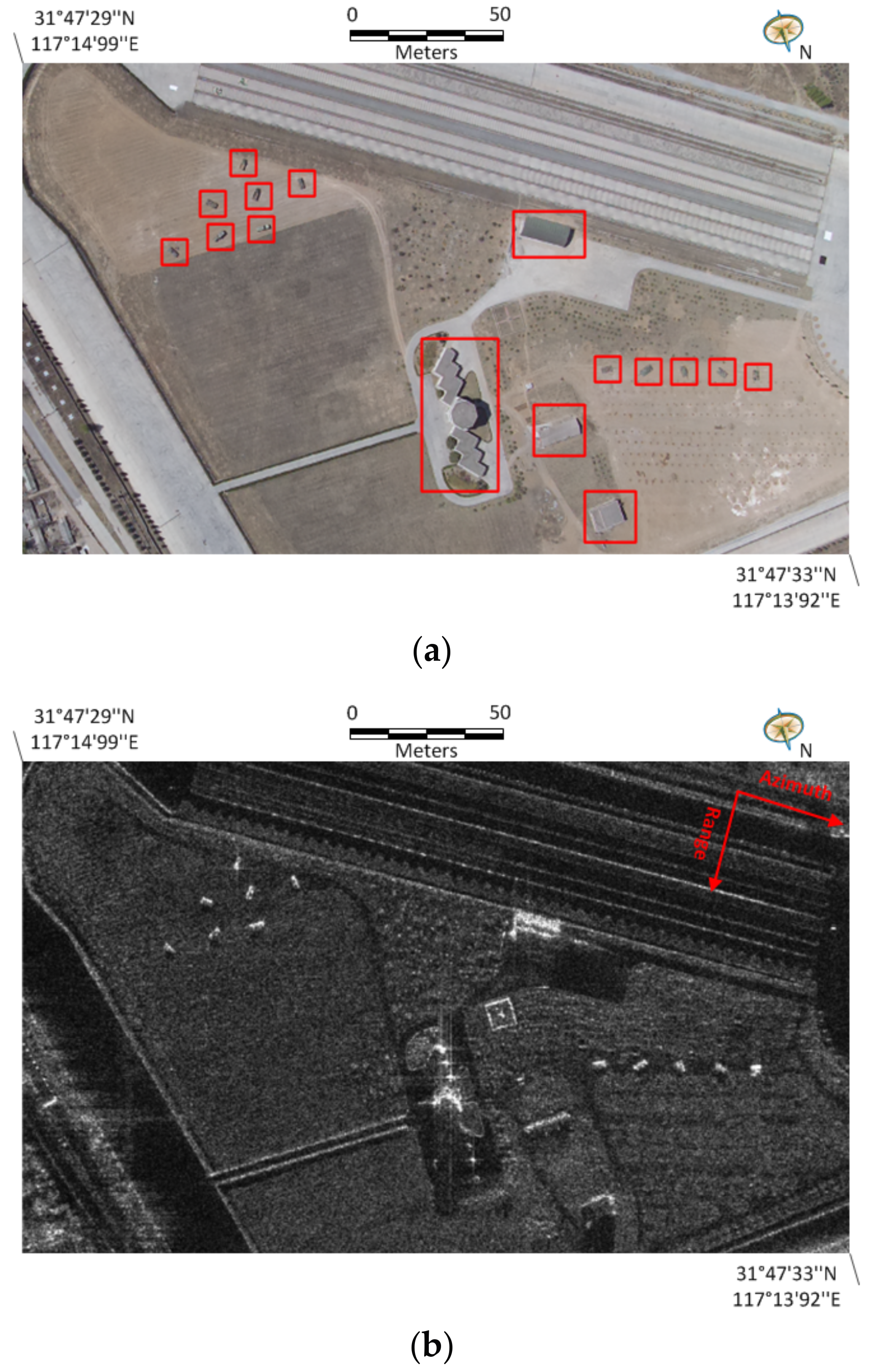
In this subsection, the first studied single-polarization SAR dataset was collected by a Chinese airborne SAR system with X band in 2005. This image was acquired in the stripmap mode HH polarization, as shown in Figure 3b, with a resolution of 0.5 m both in azimuth and range directions. The image size is 300 × 500. Figure 3a shows its corresponding optical photograph, i.e., the ground truth. As we can see, there are several vehicles, buildings, roads, and trees, leading to a complex background. From the human visual perspective, vehicles and buildings are generally of interest, and should be regarded as salient regions. They are marked with red rectangles in Figure 3a. In addition, in Figure 3b, we can see that there are some shadows near the vehicles and layovers near the buildings. These effects are common in SAR images, and we will check whether they influence the saliency map generation performance of our method in the following experiments.

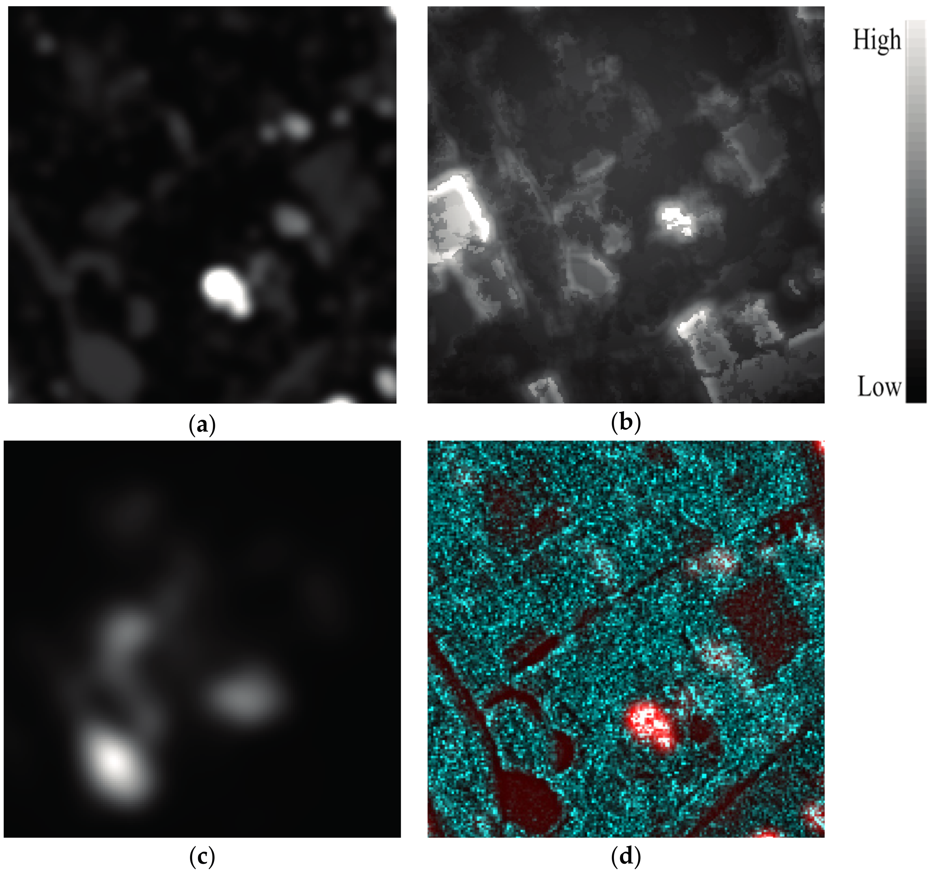
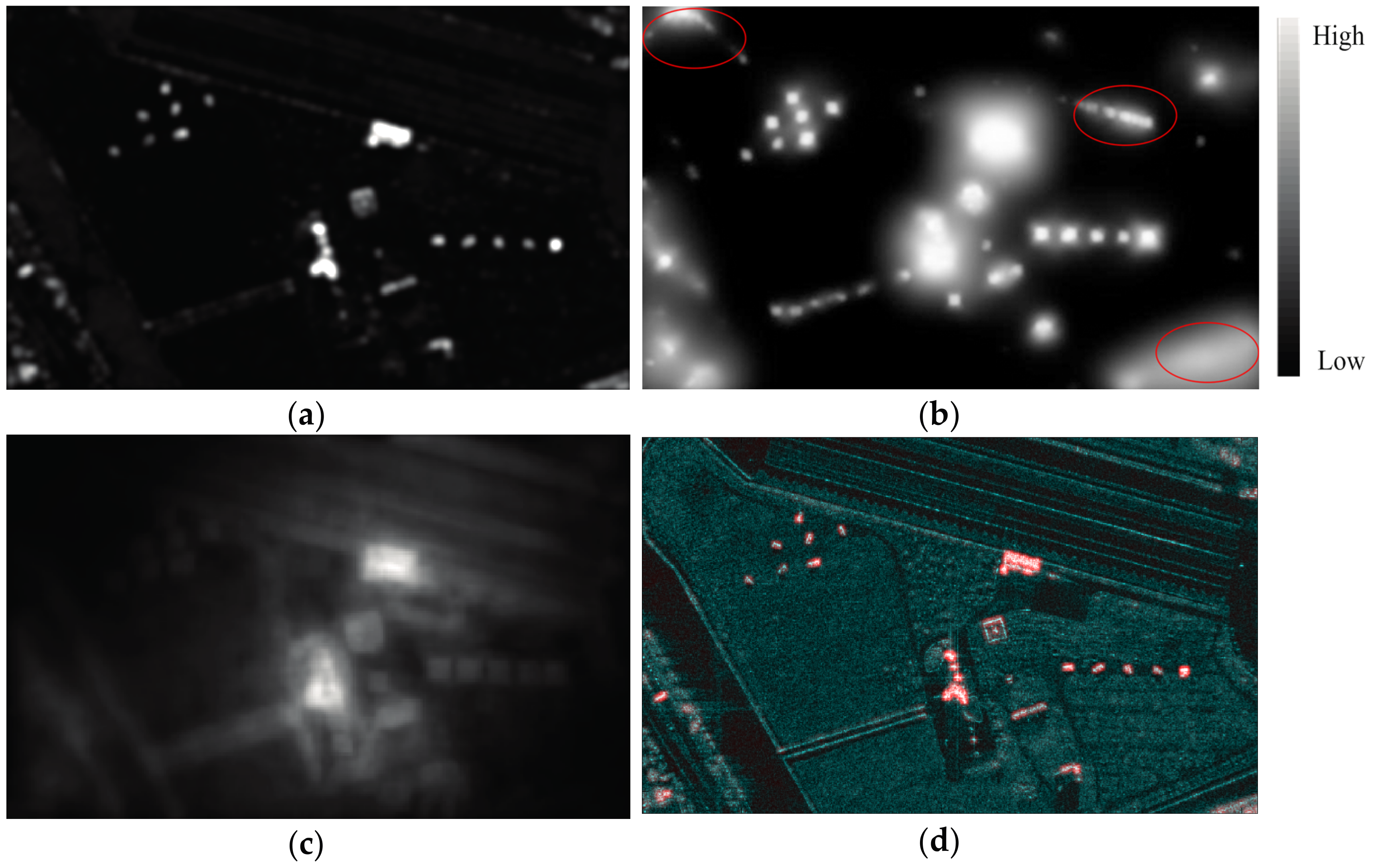
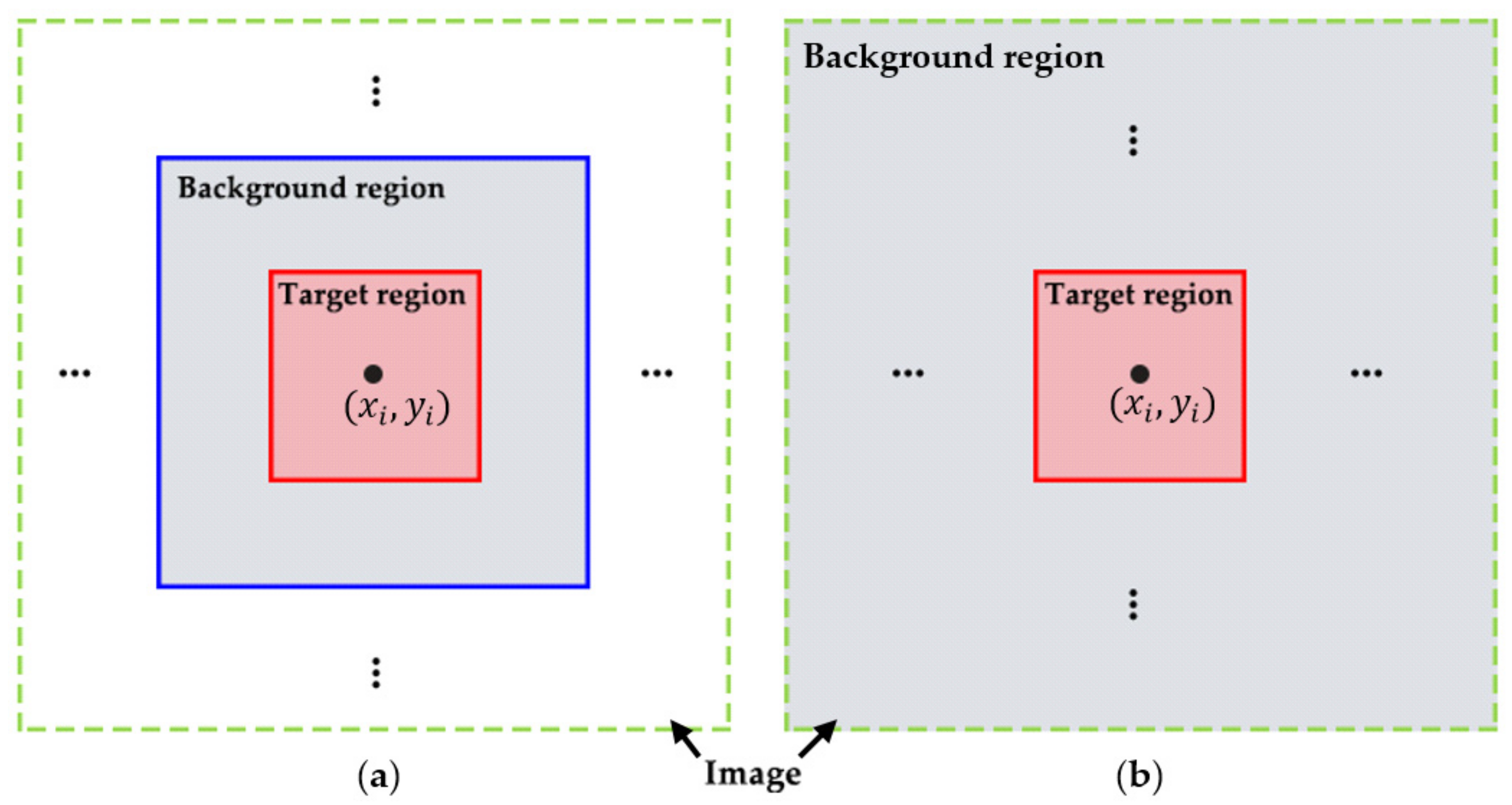
The images in Figure 4a–c give the saliency map generation results using the proposed IVSaliency and PRSaliency methods, respectively, where the pixels with high intensities are salient. The saliency map obtained by our proposed method is overlaid onto the original SAR image to form a RGB image for further validation, as shown in Figure 4d. Specifically, we use the saliency map to denote the red channel, and the original SAR image is represented by the green and blue channels. In our proposed method, the target region size is changed from 3 × 3 to 15 × 15 with step length six, i.e., the local window sizes are three, nine, and 15, respectively. The size of the background region is chosen as three times that of the target region size. From Figure 4a, we can see that the buildings and vehicles are significantly salient and attract attention. Furthermore, different salient regions can be discriminated from each other very clearly. In contrast, the trees, roads, and flat ground exhibit low saliency, which is in accordance with human visual perception. Furthermore, we can also see that shadows and layovers do not degrade the performance of saliency map generation. Figure 4b gives the result of the IVSaliency method, where we can find that the buildings and vehicles reveal extremely strong saliency values, whereas the background is not salient at all. The saliency contrast between targets and background is very significant, indicating that this method has a strong ability to measure the salient regions from SAR images. However, it can be seen that there are some obvious false alarms, such as the areas marked with red ellipses. These areas have no salient targets, but exhibit high saliency values, as shown in Figure 4b. In addition, the resolution of the saliency map is lower in comparison with that of Figure 4a. The shapes of the salient targets cannot preserve very well. The result of the PRSaliency method is given in Figure 4c, where we can observe that it is worse than the other two methods. Buildings with large sizes can exhibit apparent saliency, whereas other man-made targets, including the vehicles, have quite low saliency due to their small sizes. In addition, the resolution of the saliency map is not satisfactory, leading to the loss of salient target details. From the overlaid result displayed in Figure 4d, it can be demonstrated that our proposed method can effectively measure the salient regions and suppress the saliency of the background. Furthermore, the salient target details can be well preserved, leading to a high discrimination ability among the different targets.

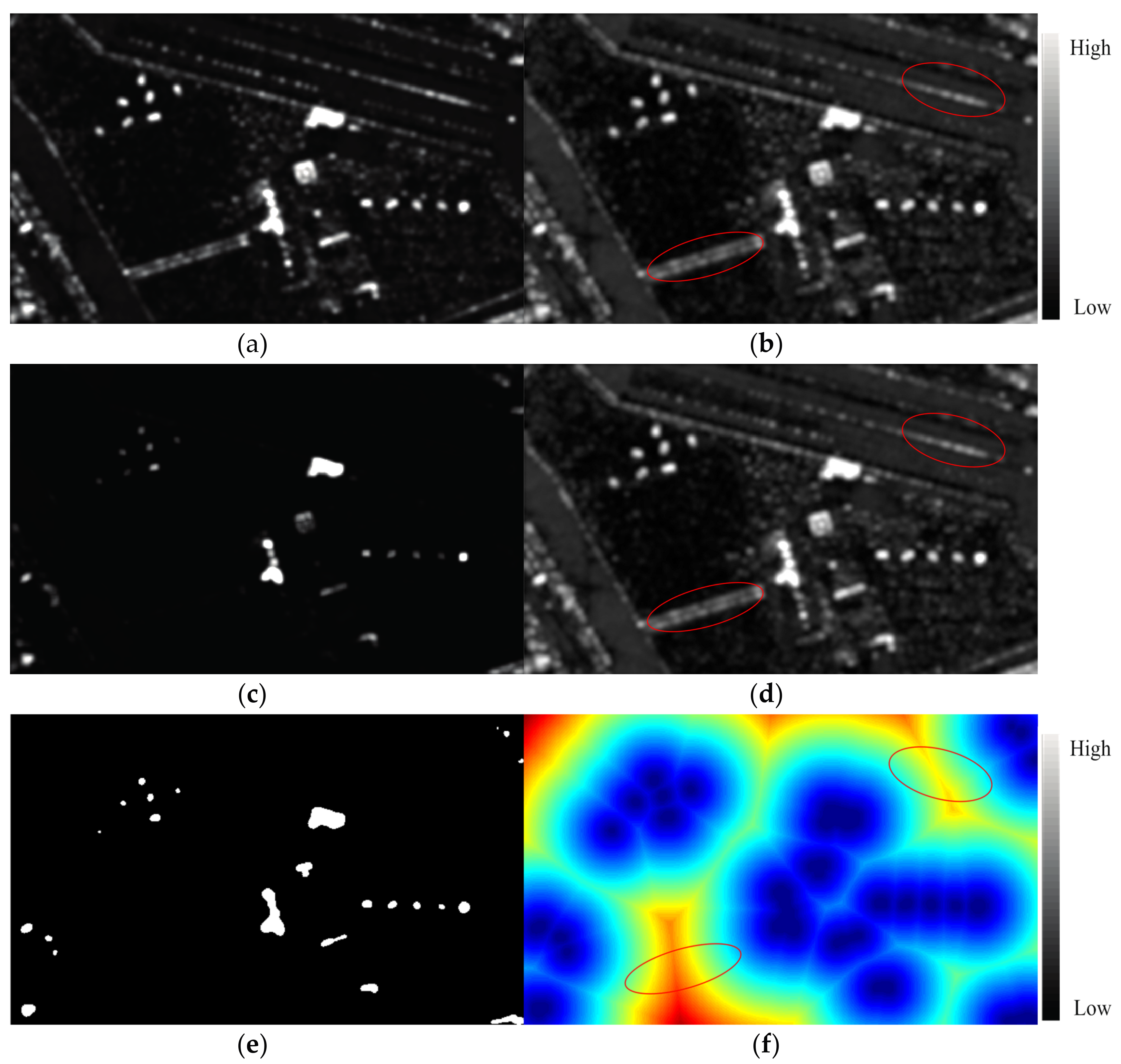
To further analyze the contributions of the different stages involved in the proposed method, we give the intermediate results in Figure 5. Figure 5a,b are the local and global saliency maps with a single scale, i.e., the target region sizes are both set as 9 × 9. Figure 5c gives the combined saliency map using the results of Figure 5a,b, according to Equation (7). What we can see from the first two images is that the salient targets in the local saliency map are more apparent and significant than those in the global saliency map. However, more false alarms exist, such as the roads and trees with relatively high backscattering. The reason is that in the estimation of the Gamma distribution parameters, the background samples in the local areas can get more accurate results than those in the global areas, since the local areas are approximately homogeneous. Therefore, the pixels with relatively high backscattering in the local regions reveal high saliency values. Thus, it can be remarked that compared to the global saliency map in Figure 5b, the local method can enhance the saliency of man-made targets at the cost of leading to high false alarms. In Figure 5c, it can be seen that the combined saliency measure considers the advantages of local and global saliency maps simultaneously. The saliency of man-made targets is enhanced, whereas that of the background is suppressed.

Figure 5d depicts the multiscale saliency map before the refinement. Compared with the saliency maps with single scale in Figure 5a–c, we can find that the multiscale processing can enhance the saliency of man-made targets. Meanwhile, the saliency of the background can be suppressed to some extent. This good performance benefits from the settings of different target region sizes, which can capture the saliency of targets with various sizes. However, we can still find some false alarms, such as the areas marked with the red ellipses, which can be further suppressed by the following refinement stage. Figure 5e gives the focus of attention regions, namely the potential targets. The distance map $d_{foci}\left(x\right)$ is shown in Figure 5f. It can be found that the pixels surrounding the focus of attention points have quite low distance values. In contrast, the roads and trees that are far away from the focus of attention points have high distance values, as shown in the red elliptic areas. According to the refinement in Equation (15), the saliency of the pixels that are far away from the focus of attention points can be further suppressed, which can be observed from the comparison between Figure 4a and Figure 5f.

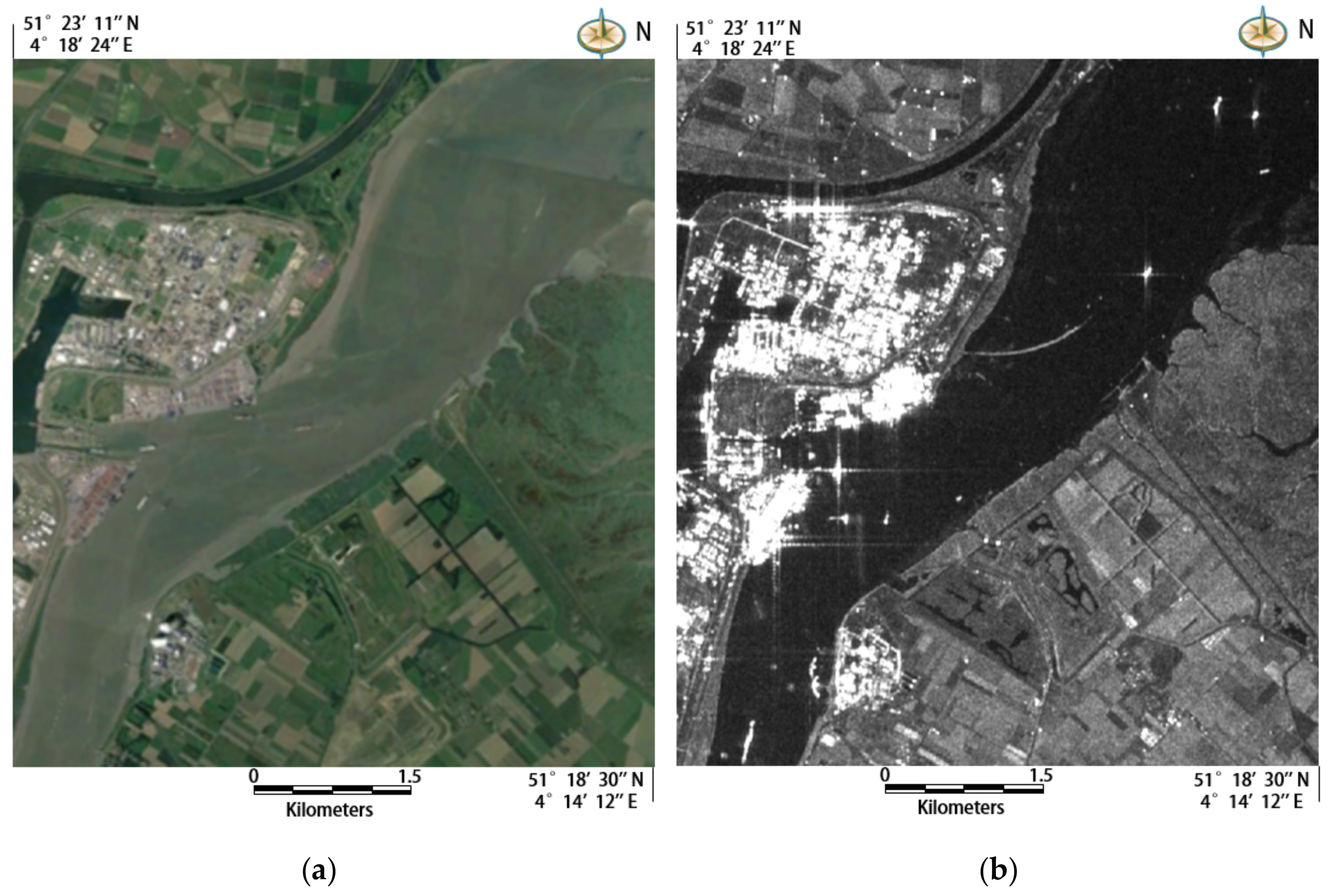
The second studied single-polarization SAR dataset was collected by the Sentinel-1 SAR sensor with C-band in 2014. The study area is located in the city of Antwerp, Belgium. This image was acquired with Level-1 ground range detected (GRD) data type, as shown in Figure 6b. It was multi-looked with a factor of six, and the resolution of resulting image is about 10 m both in azimuth and range directions. The image size is 800 × 700. Figure 6a shows its corresponding optical photograph, i.e., the ground truth. As we can see, there are high-density residential areas, low-density residential areas, rivers, farmlands, forests, and some ships on the river, which lead to a quite complex scene. From the perspective of human visual observation, ships and urban buildings are generally of interest, and should be regarded as salient objects. Note that there are some sidelobes around the ship targets and buildings, which may bring some challenges to the SAR image interpretation. In the following experiments, we will demonstrate the robustness of the sidelobes of our proposed method on saliency map generation.

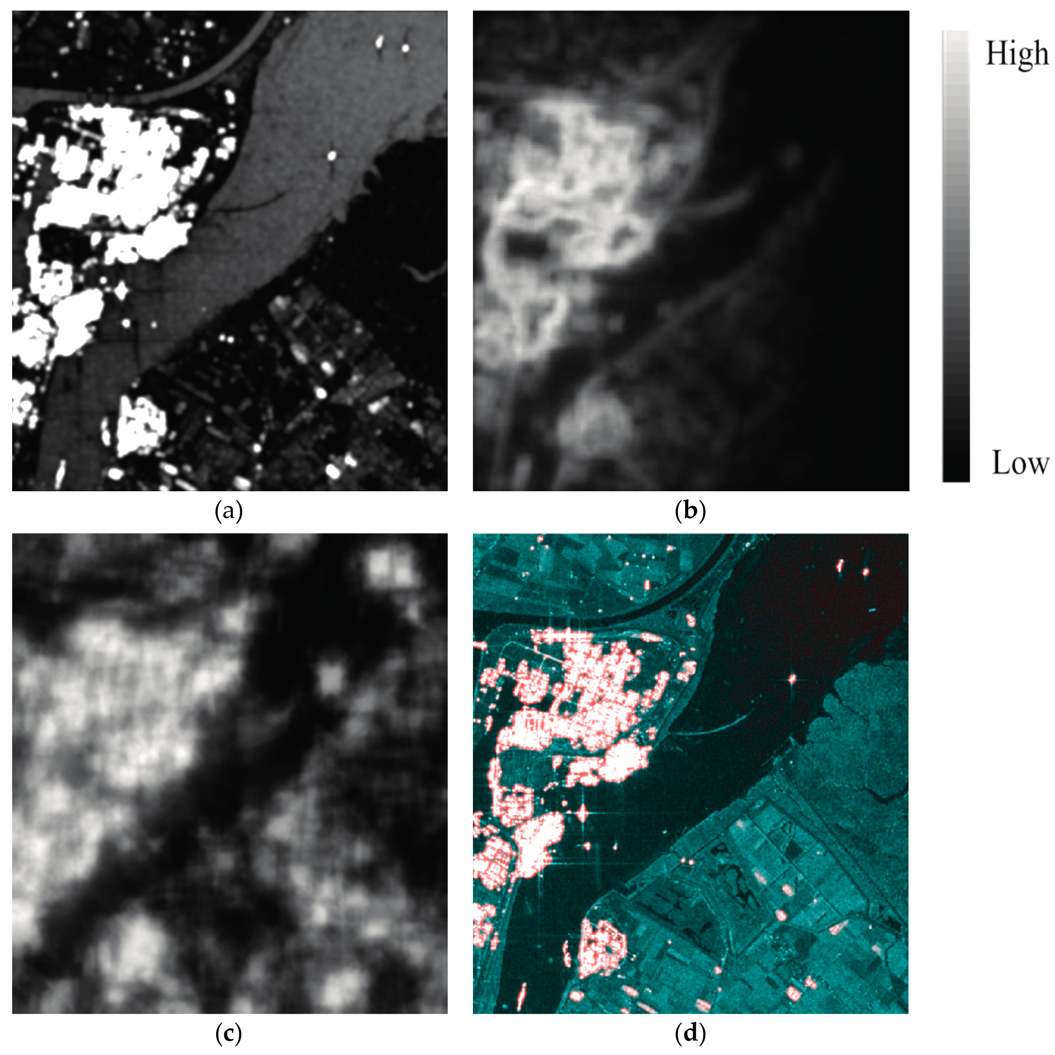
The images in Figure 7a–c present the saliency maps generated by the proposed IVSaliency and PRSaliency methods, respectively, where the pixels with high intensities are salient. Similarly, the saliency map obtained by our proposed method is overlaid onto the original SAR image to form a RGB image for further validation, as shown in Figure 7d. The target region size and background region size in the proposed method are set as before in the previous experiment. It can be seen from Figure 7a that the high-density residential areas, low-density residential areas, and ships on the river are all significantly salient, and attract human beings’ attention. In contrast, the natural areas such as farmlands, rivers, and vegetations have quite low saliency values, making the contrast between salient and nonsalient objects very clear. In addition, it also can be seen that the sidelobes around the ships and buildings do not exhibit high saliency values, indicating that the sidelobes in SAR images do not degrade the performance of the saliency map generation. Figure 7b gives the result of the IVSaliency method, where we can find that only the high-density residential buildings reveal strong saliency values, whereas the low-density residential buildings and ships are not very salient. Moreover, the resolution of the saliency map is lower in comparison with that of Figure 7a. The shapes of the salient objects cannot preserve very well. The result of the PRSaliency method is given in Figure 7c, where we can find that the high-density residential buildings and low-density residential buildings both exhibit strong salieny values. However, the ships on the river have quite low saliency due to their small sizes. In addition, the resolution of the saliency map is still not satisfactory, leading to the loss of salient target details. From the overlaid result displayed in Figure 7d, it can be demonstrated that our proposed method is still effective for measuring the salient regions of C band SAR images with complex scenes. More importantly, the proposed method is robust to the sidelobes.

4.2. Parameter Discussion

As introduced in the previous sections, two parameters exist that are involved in our proposed method, i.e., the target region size and the background region size, as shown in Figure 1. These two parameters have a close relationship with the parameter estimation of the Gamma distribution and $G_0$ distribution, which can further influence the accuracy of the saliency map generation. If the target region size is set too small, there will be some omissions. In addition, the PDF parameter estimation within the target region using few pixels is not accurate. On the other hand, if the target region size is set too large, there will exist too many false alarms. Therefore, the multiscale target region sizes are appropriate for the saliency map generation. The changes of target region size will lead to different salient scales, which is beneficial for enhancing the saliency of targets with various sizes. However, it is worth pointing out that too many salient scales will increase the computation load dramatically. Therefore, based on the aforementioned analysis, we change the target region size from 3 × 3 to 15 × 15 with step length 6. Note that the settings of maximum region size and the step length depend on the size of the potential salient target, which is related to the image resolution.

It has been stated that the background region size can be set as 3~7 times of the target region size in most of the CFAR-like algorithms [9,12,13]. In general, if we use more samples within the same region to estimate the PDF parameters, we can get a more accurate result. However, the computation load will increase significantly at the same time. Considering the efficiency of our proposed method, the background region size is set to be three times that of the target region size.

4.3. Experimental Results with PolSAR Data

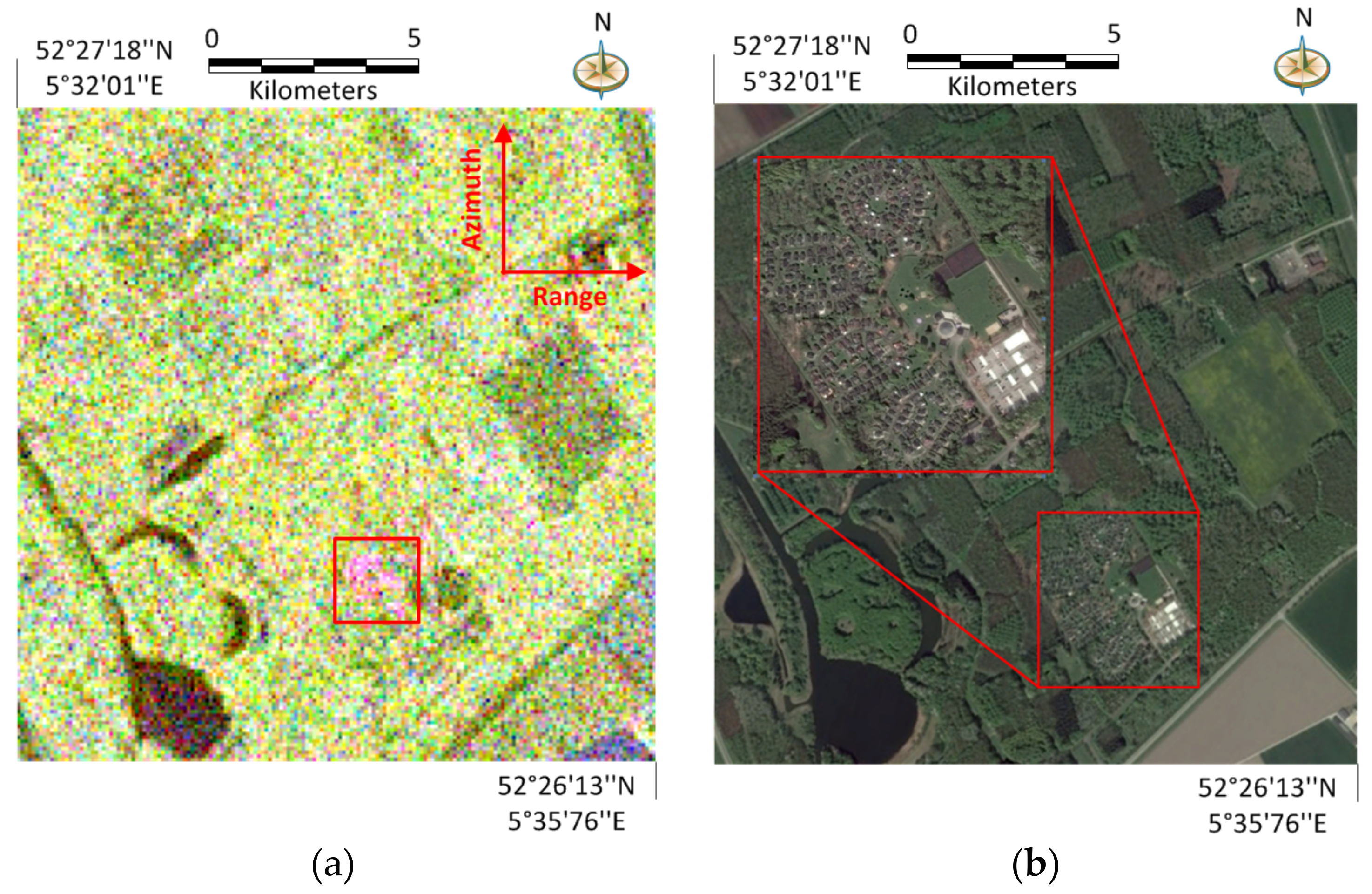
In this subsection, we utilize two PolSAR datasets to validate the effectiveness of our proposed method. The first one is acquired by the fully polarimetric Radarsat-2 C band sensor on 2 April 2008 with the fine mode over the Flevoland area, which is a city located in the center of the Netherlands. The range resolution and azimuth resolution are 5.4 m and 8.0 m, respectively. The Pauli-coded image is shown in Figure 8a, where the red channel represents double-bounce scattering, the green channel describes volume scattering, and the blue channel shows single-bounce scattering. The image rows correspond to the azimuth direction, and the columns correspond to the range direction. It can be seen that serious speckle noise exists in this PolSAR image, which makes the saliency map generation difficult to handle. Figure 8b is the corresponding optical image obtained from Google Earth. This study area covers some buildings, farms, grasslands, and lakes. Note that this test area is relatively uniform, with some buildings in the natural background. From the aspect of human visual observation, the buildings should be of interest and regarded as salient targets, which depict double-bounce scattering in the PolSAR image, as shown in the area with the red rectangle in Figure 8a. In Figure 8b, the built-up areas in the lower right area of the image are enlarged for the observation of the details. From Figure 8a,b, it is worth pointing out that not all of the buildings reveal double-bounce scattering. The reason is that the buildings that are not parallel to the radar flight path have strong cross-polarized scattering, which is similar to the scattering mechanisms of the natural areas [3,8,10]. In the PolSAR image, these buildings show a green color, and are difficult to be discriminated from forests. Therefore, these buildings are not salient in the view of human visual perception.

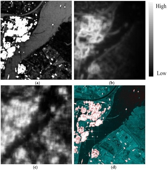
Figure 9a–c present the final saliency maps generated by using the proposed SDPolSAR and PRSaliency methods, respectively, where the pixels with high intensities are salient. Note that the parameter settings are the same as those in the previous experiment. Figure 9d shows the span image overlaid with the saliency map of our proposed method, where the red area denotes the salient region. From Figure 9a,d, we can observe that our method can effectively measure the salient regions with double-bounce scattering, such as the built-up areas. In contrast, the saliency values of the background areas, including the forests, farms, grasslands, and lakes are all suppressed. Although the PolSAR image is seriously contaminated by the multiplicative speckle noise, the saliency map does not have a lot of isolated points, making the salient region smooth. What we can see from Figure 9b is that the SDPolSAR method can also highlight the built-up areas with double-bounce scattering; however, the edges of the salient region are not very clear. Furthermore, the background also reveals relatively high saliency, such as the boundaries between different natural areas. Therefore, it can be remarked that the saliency contrast between the target and the background in Figure 9b is not as significant as that in Figure 9a. The result displayed in Figure 9c is worse than other two methods, where the saliency of the built-up areas is lower than that of the lakes. However, it is worth pointing out that the result is quite smooth, indicating that this method is quite robust to the speckle noise. From the above analysis, we can find that the proposed method can effectively measure the salient regions from PolSAR data with relatively uniform background, and thus outperforms the other two methods.

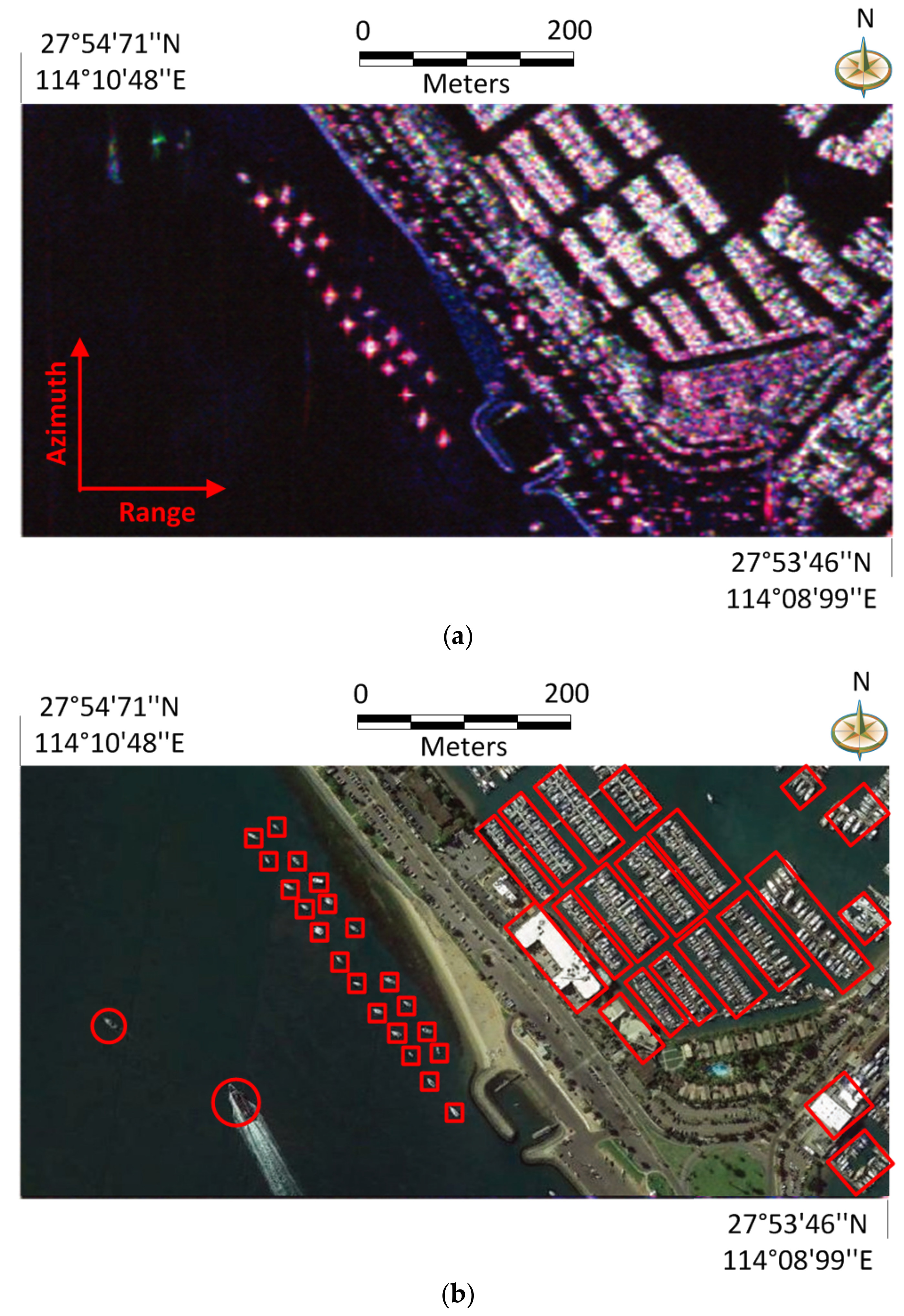
The second PolSAR dataset is acquired by the UAVSAR L-band imaging system. The study area is a harbor located in the southern California coast of the United States, as shown in Figure 10b. This area covers open water, some buildings, isolated boats, and man-made grounds, which is a complex image scene. Figure 10a displays the full polarimetric SAR image with Pauli-color coding, where the rows denote the azimuth direction and the columns represent the range direction. The multilook complex data have a resolution with 7.2 m in the azimuth direction and 5 m in the range direction. From the perspective of human visual perception, the boats and buildings are of interest, and should be regarded as salient objects, which are marked with red rectangles in Figure 10b. Due to the relatively low resolution, the vehicles on the road are too small to be regarded as salient objects. Note that there are two ships in Figure 10b, but they disappear in Figure 10a, as depicted in the two red circles. It is worth pointing out that the optical image is acquired from Google Earth, which has a different date than that of the PolSAR image; therefore, the two ships may move out of this place. They are ignored in the following comparison analysis.

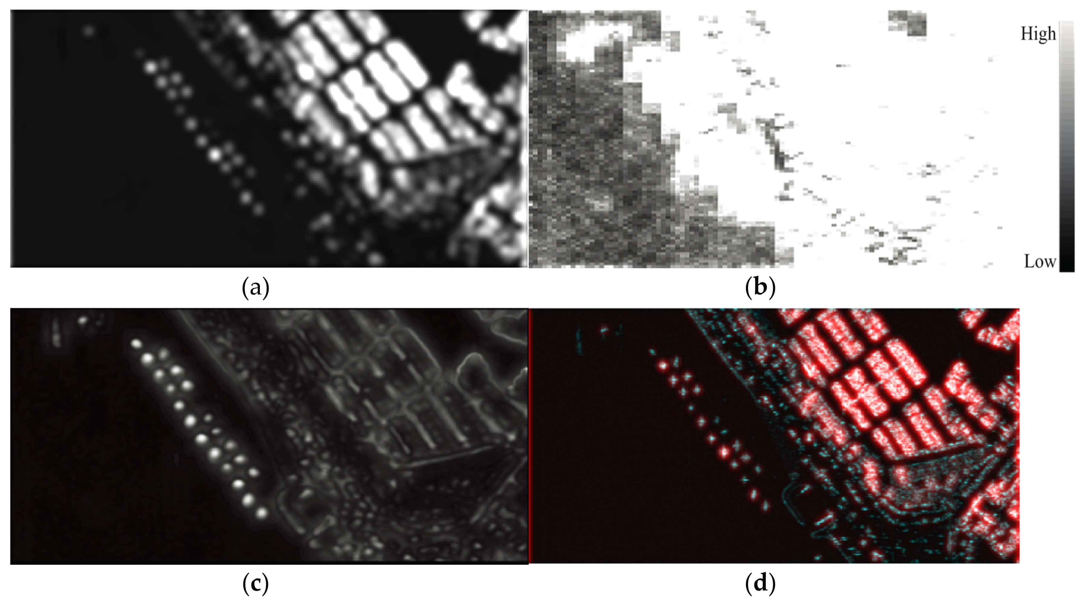
Figure 11a–c show the saliency maps of the three methods, respectively. Figure 11d overlays the proposed detection result on the span image, where the red regions denote the salient targets. What we can see from Figure 11a,d is that our proposed method can obtain most of the salient targets, including the isolated and assembled boats. In addition, the buildings inside the harbor can also be effectively highlighted. The saliency of the background areas is suppressed very well, which makes the saliency map smooth and clear. Nevertheless, some small targets have relatively low saliency values, making them difficult to be measured. The reason is that the target sizes are smaller than the minimal target region size, leading to saliency measure omissions of the targets. In Figure 11b, we can find that the result of the SDPolSAR method is not satisfactory. The resolution of the saliency map is bad, and the salient targets cannot be clearly discriminated. Furthermore, the saliency of the background is not suppressed well. Therefore, this method is not very effective for the saliency map generation from the complex heterogeneous image scenes. From Figure 11c, it can be seen that the result of the PRSaliency method is fine, where the isolated boats can be well detected. In addition, the saliency of the background is also suppressed. However, this method cannot measure the saliency of the assembled boats and buildings, making the result worse than our proposed method. From the comparison of these methods, it can be found that the proposed approach can well highlight the salient targets from the PolSAR image with a complex heterogeneous background. The targets exhibit higher saliency than the backgrounds, and also can be clearly discriminated from each other.

4.4. Performance Evaluation and Comparison

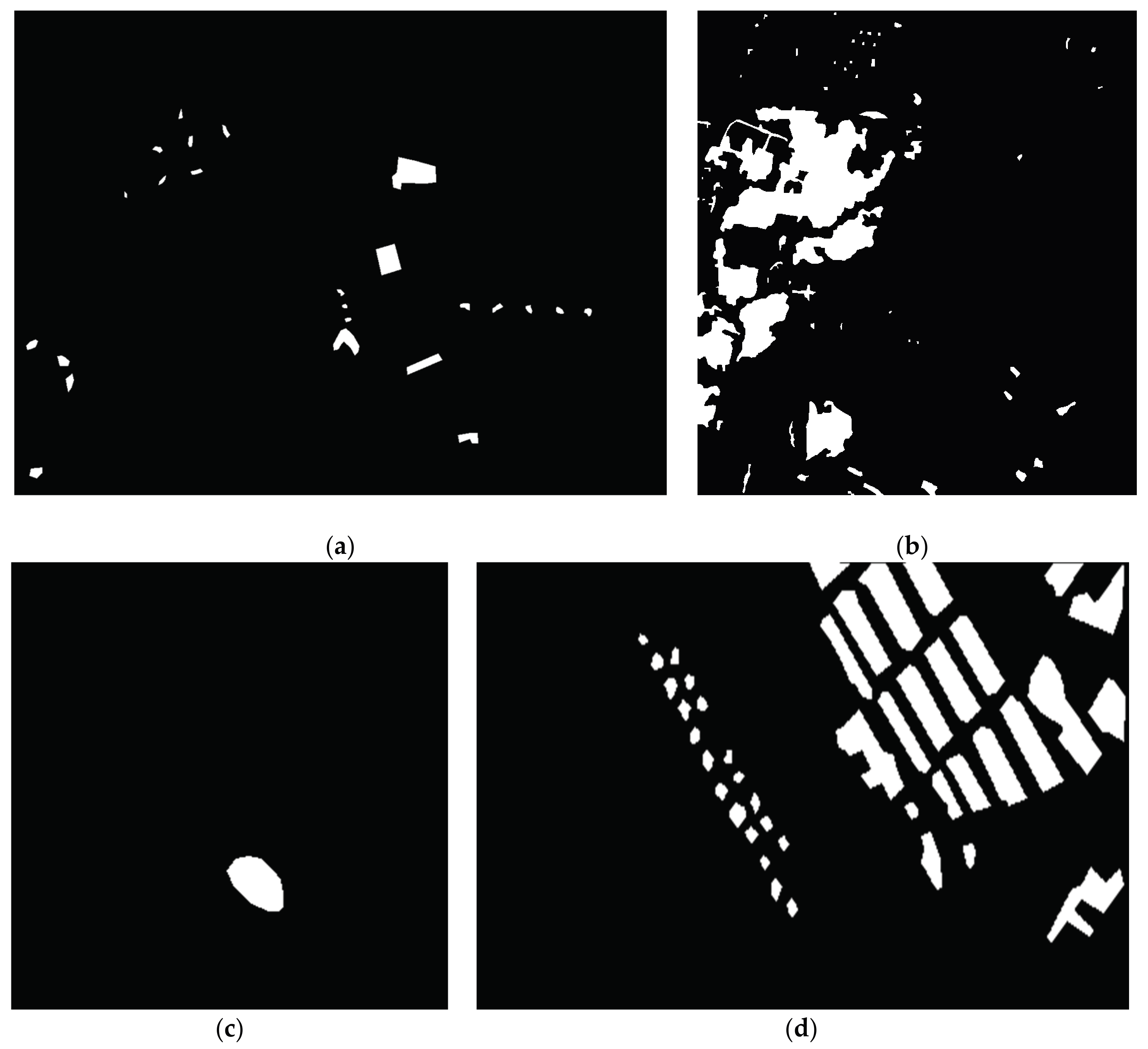
There are few studies that focus on quantitative evaluation indicators for saliency map generation. As we stated in the Introduction section, saliency is a measure of prominent characteristics that can be used to discriminate targets from backgrounds. Therefore, our proposed approach can be extended to salient target detection for SAR and PolSAR images, and the detection accuracy analysis can be used to evaluate the performance of the saliency map. It is worth pointing out that the saliency map also can be used in other applications, such as the image segmentation. Therefore, the evaluation indicators for image segmentation also can be used to measure the saliency map generation performance. Since this work starts from the target detection application and further proposes saliency map generation methods for SAR and PolSAR images, we adopt the target detection accuracy measures to quantitatively evaluate the saliency map generation performance of different methods. Salient targets can be detected by simply thresholding the saliency map. In this paper, we set the threshold to 0.7 for simplicity. To quantitatively evaluate the performance of different saliency map generation methods, we compare the target detection results using various saliency maps with respect to human-annotated “ground truth”.

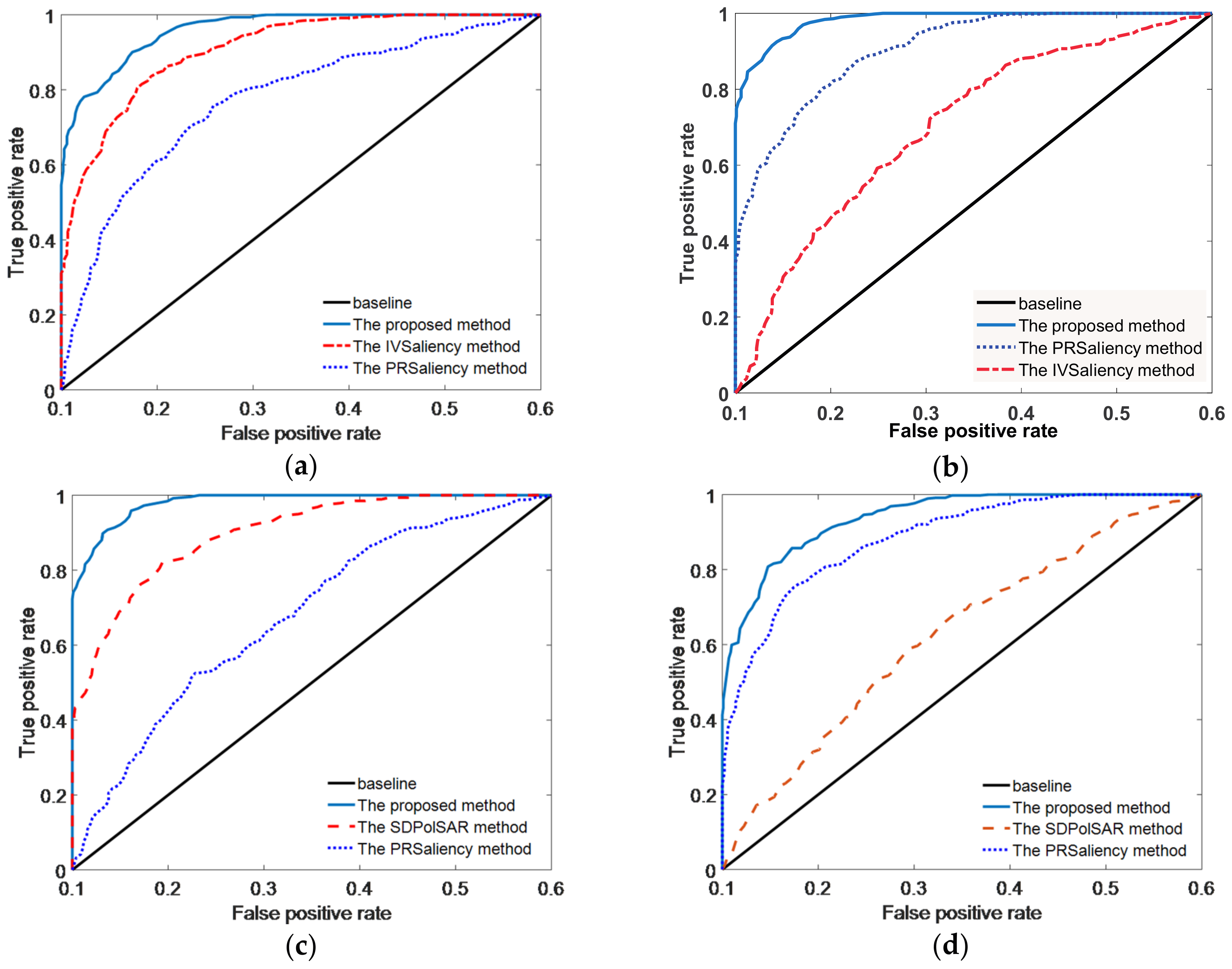
Figure 12 gives the ground truth maps of salient target detection using above four datasets respectively, which are all annotated with human eye observation. Figure 13 depicts the receiver operating characteristic (ROC) curves of different methods using four datasets. An ROC graph depicts relative tradeoffs between benefits (true positives) and costs (false positives). Methods on the upper left-hand side of an ROC graph are generally regarded as excellent. From the four ROC graphs depicted in Figure 13, we find that our proposed method can achieve the best salient target detection performance in both SAR and PolSAR images among different approaches. For the sake of further comparison, the AUCs (i.e., areas under the curve of ROC, the higher the AUC, the better the detector) of different methods are given in

Table 1. Area under the curve (AUC) results of different methods.

	X Band SAR Image	Sentinel-1 C Band SAR Image	Radarsat-2 C Band Image	UAVSAR L Band Image
The proposed method	0.9756	0.9833	0.9879	0.9512
The IVSaliency method	0.9347	0.7241
The PRSaliency method	0.8435	0.8012	0.7651	0.9323
The SDPolSAR method			0.9014	0.7345

. The method has a better saliency detection performance if its AUC is close to one.

From Figure 13 and Table 1, we can find that the IVSaliency method can achieve a satisfactory result with the X band SAR image compared to the proposed approach. However, it cannot perform so well with the Sentinel-1 C band SAR image. In addition, it cannot be applicable to the PolSAR images. The PRSaliency method can be applied to both single-polarization SAR images and PolSAR images. It performs well in the UAVSAR L band image, but is not satisfactory in the X band and C band SAR images, and the Radarsat-2 C band PolSAR image. Therefore, it can be stated that this method is suitable for saliency map generation in the PolSAR image with a relatively complex background. The performance of the SDPolSAR method is comparable with other methods in the saliency map generation of the PolSAR image with a uniform background (e.g., Radarsat-2 C band image). Nevertheless, it performs much worse than the other methods in the PolSAR image with a complex heterogeneous background (UAVSAR L band image). It can be found that the proposed saliency map generation method performs well both with single-polarization SAR images and PolSAR images. Furthermore, the generated saliency maps are satisfactory with and without the complex background. The saliency map accuracy can achieve above 95% with four datasets, which is about 5–20% higher than other methods.

Table 2. Time costs of saliency detection using different methods (seconds).

	X-Band SAR Image 300 × 500	Sentinel-1 C-Band SAR Image 800 × 700	Radarsat-2 C-Band Image 300 × 300	UAVSAR L-Band Image 250 × 600
The proposed method	20.14	52.36	28.54	36.15
The IVSaliency method	13.25	30.19
The PRSaliency method	12.14	26.92	10.38	18.57
The SDPolSAR method			18.17	25.78

gives the time costs of saliency map generation using different methods. All of the experiments are implemented using MATLAB language on a laptop with an Intel Core i7-6700HQ CPU with frequency of 2.6 GHz and 32-GB RAM. The sizes of the X-band SAR, Sentinel-1 C-band, Radarsat-2 C-band, and UAVSAR L-band images are 300 × 500, 800 × 700, 300 × 300, and 250 × 600, respectively. From Table 2, we can see that the computational cost of our proposed approach is higher than other methods. The time cost mainly comes from the parameter estimation of PDFs. The PRSaliency method runs fast among these methods, thanks to the quick computation of the pattern recurrence. Note that although our method can achieve satisfactory saliency map generation results, the efficiency should be further improved in the future.

5. Conclusions

This paper proposes a saliency map generation method for SAR and PolSAR images based on Bayes theory and a heterogeneous clutter model. The ratio of the probability density functions in the target and background areas is utilized to define the saliency, which also considers the local and global information. For saliency map generation in SAR images, the Gamma and $G_0$ distributions are utilized to model the salient and nonsalient areas. For PolSAR images, the Wishart and polarimetric $G_0$ distributions are adopted. Therefore, this proposed method can highlight the salient regions from SAR and PolSAR images with and without a complex background. Furthermore, multiscale saliency enhancement is conducted to measure the saliency of targets with different sizes. The result is further refined by considering the image immediate context. The proposed method is firstly validated on an X-band SAR image and a Sentinel-1 C-band SAR image, and compared with respect to existing methods such as IVSaliency and PRSaliency. It is then tested with Radarsat-2 C-band and UAVSAR L-band PolSAR images, and compared with SDPolSAR and PRSaliency methods. The results of four datasets with different frequencies demonstrate that our proposed method performs best in terms of robustly highlighting salient targets with and without the presence of a complicated background. Furthermore, the shadows, layovers, and sidelobes in the SAR images do not degrade the performance of saliency map generation, which increases the actual applicability and portability of the proposed methodology.

Future work will mainly focus on the improvement of computational efficiency and further applications using the saliency map. In addition, the saliency of buildings not parallel to the radar flight path in PolSAR images should be enhanced by considering the scattering mechanisms, which is beneficial for discriminating them from natural areas.

References

1. Soergel, U. Radar Remote Sensing of Urban Areas; Springer: Berlin, Germany, 2010. [Google Scholar]
2. Lee, J.-S.; Pottier, E. Polarimetric Radar Imaging: From Basics to Applications; CRC Press: Boca Raton, FL, USA, 2009. [Google Scholar]
3. Xiang, D.; Tang, T.; Ban, Y.; Su, Y. Man-made target detection from polarimetric SAR data via nonstationarity and asymmetry. IEEE J. Sel. Top. Appl. Earth Obs. 2016, 9, 1459–1469. [Google Scholar] [CrossRef]
4. Yu, W.; Wang, Y.; Liu, H.; He, J. Superpixel-based CFAR target detection for high-resolution SAR images. IEEE Geosci. Remote Sens. Lett. 2016, 13, 730–734. [Google Scholar] [CrossRef]
5. Tu, S.; Su, Y. Fast and accurate target detection based on multiscale saliency and active contour model for high-resolution SAR images. IEEE Trans. Geosci. Remote Sens. 2016, 54, 5729–5744. [Google Scholar] [CrossRef]
6. Zhang, L.; Zou, B.; Tang, W. Similarity-enhanced target detection algorithm using polarimetric sar images. Int. J. Remote Sens. 2012, 33, 6149–6162. [Google Scholar] [CrossRef]
7. An, W.; Xie, C.; Yuan, X. An improved iterative censoring scheme for CFAR ship detection with SAR imagery. IEEE Trans. Geosci. Remote Sens. 2014, 52, 4585–4595. [Google Scholar]
8. Wu, W.; Guo, H.; Li, X. Urban area man-made target detection for PolSAR data based on a nonzero-mean statistical model. IEEE Geosci. Remote Sens. Lett. 2014, 11, 1782–1786. [Google Scholar] [CrossRef]
9. Gao, G. A parzen-window-kernel-based CFAR algorithm for ship detection in SAR images. IEEE Geosci. Remote Sens. Lett. 2011, 8, 557–561. [Google Scholar] [CrossRef]
10. Chen, S.; Sato, M. Tsunami damage investigation of built-up areas using multitemporal spaceborne full polarimetric SAR images. IEEE Trans. Geosci. Remote Sens. 2013, 51, 1985–1997. [Google Scholar] [CrossRef]
11. Di Bisceglie, M.; Galdi, C. CFAR detection of extended objects in high-resolution SAR images. IEEE Trans. Geosci. Remote Sens. 2005, 43, 833–843. [Google Scholar] [CrossRef]
12. Gandhi, P.P.; Kassam, S.A. Analysis of CFAR processors in homogeneous background. IEEE Trans. Aerosp. Electron. Syst. 1988, 24, 427–445. [Google Scholar] [CrossRef]
13. Smith, M.E.; Varshney, P.K. VI-CFAR: A novel CFAR algorithm based on data variability. In Proceedings of the IEEE National Radar Conference, Syracuse, NY, USA, 13–15 May 1997; IEEE: Piscataway, NJ, USA, 1997; pp. 263–268. [Google Scholar]
14. Kaplan, L.M. Improved SAR target detection via extended fractal features. IEEE Trans. Aerosp. Electron. Syst. 2001, 37, 436–451. [Google Scholar] [CrossRef]
15. Tello, M.; López-Martínez, C.; Mallorqui, J.J. A novel algorithm for ship detection in SAR imagery based on the wavelet transform. IEEE Geosci. Remote Sens. Lett. 2005, 2, 201–205. [Google Scholar] [CrossRef]
16. Brekke, C.; Anfinsen, S.N.; Larsen, Y. Subband extraction strategies in ship detection with the subaperture crosscorrelation magnitude. IEEE Geosci. Remote Sens. Lett. 2013, 10, 786–790. [Google Scholar] [CrossRef]
17. Marino, M.S.-F.; Hajnsek, I.; Ouchi, K. Ship detection with analysis of synthetic aperture radar: A comparison of new and well-known algorithms. Remote Sens. 2015, 7, 5416–5439. [Google Scholar] [CrossRef]
18. Iervolino, P.; Guida, R. A novel ship detector based on the generalized-likelihood ratio test for SAR imagery. IEEE J. Sel. Top. Appl. Earth Obs. 2017, 10, 3616–3630. [Google Scholar] [CrossRef]
19. Yu, Y.; Wang, B.; Zhang, L. Hebbian-based neural networks for bottom-up visual attention and its applications to ship detection in sar images. Neurocomputing 2011, 74, 2008–2017. [Google Scholar] [CrossRef]
20. Tang, T.; Xiang, D.; Xie, H. Multiscale salient region detection and salient map generation for synthetic aperture radar image. J. Appl. Remote Sens. 2014, 8, 083501. [Google Scholar] [CrossRef]
21. Wang, H.; Xu, F.; Chen, S. Saliency detector for SAR images based on pattern recurrence. IEEE J. Sel. Top. Appl. Earth Obs. Remote Sens. 2016, 9, 2891–2900. [Google Scholar] [CrossRef]
22. Zhang, Q.; Wu, Y.; Zhao, W.; Wang, F.; Fan, J.; Li, M. Multiple-scale salient-region detection of SAR image based on gamma distribution and local intensity variation. IEEE Geosci. Remote Sens. Lett. 2014, 11, 1370–1374. [Google Scholar] [CrossRef]
23. Zhang, Q.; Wu, Y.; Wang, F.; Fan, J.; Zhang, L.; Jiao, L. Anisotropic-scale-space-based salient-region detection for SAR images. IEEE Geosci. Remote Sens. Lett. 2016, 13, 457–461. [Google Scholar] [CrossRef]
24. Zhang, X.; Meng, H.; Ma, Z.; Tian, X. SAR image despeckling by combining saliency map and threshold selection. Int. J. Remote Sens. 2013, 34, 7854–7873. [Google Scholar] [CrossRef]
25. Zheng, Y.; Jiao, L.; Liu, H.; Zhang, X.; Hou, B.; Wang, S. Unsupervised saliency-guided SAR image change detection. Pattern Recognit. 2017, 61, 309–326. [Google Scholar] [CrossRef]
26. Itti, L.; Koch, C.; Niebur, E. A model of saliency-based visual attention for rapid scene analysis. IEEE Trans. Pattern Anal. Mach. Intell. 1998, 20, 1254–1259. [Google Scholar] [CrossRef]
27. Harel, J.; Koch, C.; Perona, P. Graph-based visual saliency. In Proceedings of the 20th Annual Conference on Neural Information Processing Systems, Vancouver, BC, Canada, 4–7 December 2006; pp. 545–552. [Google Scholar]
28. Jin, S.; Wang, S.; Li, X.; Jiao, L.; Zhang, J.A.; Shen, D. A salient region detection and pattern matching-based algorithm for center detection of a partially covered tropical cyclone in a SAR image. IEEE Trans. Geosci. Remote Sens. 2017, 55, 280–291. [Google Scholar] [CrossRef]
29. Jager, M.; Hellwich, O. Saliency and salient region detection in SAR polarimetry. In Proceedings of the IEEE International Geoscience and Remote Sensing Symposium, Seoul, Korea, 29–29 July 2005; pp. 2791–2794. [Google Scholar]
30. Huang, X.; Huang, P.; Dong, L.; Song, H.; Yang, W. Saliency detection based on distance between patches in polarimetric SAR images. In Proceedings of the International Geoscience and Remote Sensing Symposium, Quebec City, QC, Canada, 13–18 July 2014; pp. 4572–4575. [Google Scholar]
31. Gao, G. Statistical modeling of SAR images: A survey. Sensors 2010, 10, 775–795. [Google Scholar] [CrossRef] [PubMed]
32. Deng, X.; López-Martínez, C.; Chen, J.; Han, P. Statistical modeling of polarimetric SAR data: A survey and challenges. Remote Sens. 2017, 9, 348. [Google Scholar] [CrossRef]
33. Marques, R.C.P.; Medeiros, F.N.; Nobre, J.S. SAR image segmentation based on level set approach and G0 model. IEEE Trans. Pattern Anal. Mach. Intell. 2012, 34, 2046–2057. [Google Scholar] [CrossRef] [PubMed]
34. Frery, A.C.; Muller, H.-J.; Yanasse, C.C.F.; Sant’Anna, S.J.S. A model for extremely heterogeneous clutter. IEEE Trans. Geosci. Remote Sens. 1997, 35, 648–659. [Google Scholar] [CrossRef]
35. Goferman, S.; Zelnik-Manor, L.; Tal, A. Context-aware saliency detection. IEEE Trans. Pattern Anal. Mach. Intell. 2012, 34, 1915–1926. [Google Scholar] [CrossRef] [PubMed]
36. Freitas, C.C.; Frery, A.C.; Correia, A.H. The polarimetric G distribution for SAR data analysis. Environmetrics 2005, 16, 13–31. [Google Scholar] [CrossRef]
Figure 1. Target and background regions (salient and nonsalient regions) used for the estimation of two probability density functions (PDFs). (a) Regions for the calculation of the local saliency measure; (b) Regions for the calculation of the global saliency measure.
Remotesensing 09 01290 g001
Figure 2. Framework of the proposed saliency map generation procedure. (a) Synthetic aperture radar (SAR) image saliency map generation; (b) Polarimetric SAR (PolSAR) image saliency generation.
Remotesensing 09 01290 g002
Figure 3. First study area and single-polarization SAR dataset with X-band. (a) Optical image from Google Earth. The red rectangles denote salient regions through human visual perception; (b) HH polarization SAR image with X-band.
Remotesensing 09 01290 g003
Figure 4. Saliency map generation results of different methods. (a) The proposed method; (b) The IVSaliency method; (c) The PRSaliency method; (d) Original SAR image overlaid with the salient map of (a), where the red regions are salient.
Remotesensing 09 01290 g004
Figure 5. The intermediate results of our proposed saliency map generation algorithm. (a) Local saliency map with single scale; (b) Global saliency map with single scale; (c) Combined saliency map with single scale; (d) Multiscale saliency map before refinement; (e) Focus of attention points at single scale; (f) Distance image d foci ( x ) at single scale.
Remotesensing 09 01290 g005
Figure 6. The study area and Sentinel-1 SAR dataset with C band. (a) Optical image from Google Earth; (b) HH polarization SAR image with C band.
Remotesensing 09 01290 g006
Figure 7. Saliency map generation results of different methods using the Sentinel-1 dataset. (a) The proposed method; (b) The IVSaliency method; (c) The PRSaliency method; (d) Original SAR image overlaid with the saliency map of (a), where the red regions are salient.
Remotesensing 09 01290 g007
Figure 8. The study area and Radarsat-2 dataset. (a) Pauli-coded image with C-band (red: HH − VV, green: HV, blue: HH + VV); (b) Optical image from Google Earth, where the red area in the upper left image is the enlarged result of the lower right area.
Remotesensing 09 01290 g008
Figure 9. Saliency map generation results of Radarsat-2 C-band data with uniform background. (a) The proposed method; (b) The SDPolSAR method; (c) The PRSaliency method; (d) Span image overlaid with the saliency map of (a), where the red regions are salient.
Remotesensing 09 01290 g009
Figure 10. Third study area and UAVSAR dataset. (a) Pauli-coded image with L-band (red: HH − VV, green: HV, blue: HH + VV); (b) Optical image from Google Earth. The areas with red rectangles represent targets of interest.
Remotesensing 09 01290 g010
Figure 11. Saliency map generation results of the UAVSAR L-band data with complex image scenes. (a) The proposed method; (b) The SDPolSAR method; (c) The PRSaliency method; (d) Span image overlaid with the saliency map of (a), where the red regions are salient.
Remotesensing 09 01290 g011
Figure 12. Human-annotated ground truth of salient target detection. (a) X-band SAR image; (b) Sentinel-1 C-band SAR image; (c) Radarsat-2 C-band PolSAR image; (d) UAVSAR L-band PolSAR image.
Remotesensing 09 01290 g012
Figure 13. Receiver operating characteristic (ROC) curves of various methods using different datasets. (a) X-band SAR image; (b) Sentinel-1 C-band SAR image; (c) Radarsat-2 C-band PolSAR image; (d) UAVSAR L-band PolSAR image.
Remotesensing 09 01290 g013