Spatiotemporal Variability of Land Surface Phenology in China from 2001–2014

Abstract

Land surface phenology is a highly sensitive and simple indicator of vegetation dynamics and climate change. However, few studies on spatiotemporal distribution patterns and trends in land surface phenology across different climate and vegetation types in China have been conducted since 2000, a period during which China has experienced remarkably strong El Niño events. In addition, even fewer studies have focused on changes of the end of season (EOS) and length of season (LOS) despite their importance. In this study, we used four methods to reconstruct Moderate Resolution Imaging Spectroradiometer (MODIS) Enhanced Vegetation Index (EVI) dataset and chose the best smoothing result to estimate land surface phenology. Then, the phenophase trends were analyzed via the Mann-Kendall method. We aimed to assess whether trends in land surface phenology have continued since 2000 in China at both national and regional levels. We also sought to determine whether trends in land surface phenology in subtropical or high altitude areas are the same as those observed in high latitude areas and whether those trends are uniform among different vegetation types. The result indicated that the start of season (SOS) was progressively delayed with increasing latitude and altitude. In contrast, EOS exhibited an opposite trend in its spatial distribution, and LOS showed clear spatial patterns over this region that decreased from south to north and from east to west at a national scale. The trend of SOS was advanced at a national level, while the trend in Southern China and the Tibetan Plateau was opposite to that in Northern China. The transaction zone of the SOS within Northern China and Southern China occurred approximately between 31.4°N and 35.2°N. The trend in EOS and LOS were delayed and extended, respectively, at both national and regional levels except that of LOS in the Tibetan Plateau, which was shortened by delayed SOS onset more than by delayed EOS onset. The absolute magnitude of SOS was decreased after 2000 compared with previous studies, and the phenophase trends are species specific.

1. Introduction

Vegetation phenology and variation in vegetation phenology are highly sensitive indicators of climate change that can yield important insights into nutrient cycles and energy exchange processes at different scales [1]. Rapid shifts in vegetation phenology have strong impacts on vegetation growth, plant competition, ecosystem functions, and carbon balance [2]. The study of vegetation phenology not only provides an understanding of the ecophysiological processes of ecosystems, but can also reveal transformations occurring under climate change [2]. Therefore, accurate prediction and characterization of vegetation phenology are necessary to understand how the impacts of climate change vary across space and time.

Vegetation phenology is currently studied mainly via four methods: bioclimatic models [3,4,5], visible digital camera imaging [6,7], field observation, and satellite estimates. Field observations have been widely and successfully conducted, providing detailed information at the species level based on individual plant observations across many countries [8], and observation networks have been established to support these ongoing observations [9,10]. A large number of studies have been conducted to observe vegetation phenology at short- and/or long-term scales across many regions [11], but these observations have focused mainly on developmental switches within individual species [12] and cannot reveal integrative phenology patterns on the biome or broader scale, and this research is often time inefficient and labor intensive [1,13]. Alternatively, satellite-based methods, which rely on vegetation indexes (e.g., NDVI) provide a powerful, integrative, and objective tool for monitoring and characterizing key phenological metrics (such as the start of the season (SOS), end of the season (EOS), and length of the season (LOS)) at regional and global scales across long time-series, serving as an excellent complement to the shortage of field observations [14]. Since the launch of satellite sensors such as the Advanced Very High Resolution Radiometer (AVHRR), land surface phenology has been intensively studied using vegetation indexes at regional and global scales (see [13] for details). However, this tool’s spatial resolution is too coarse (mostly reported at an 8-km scale) to accurately estimate land surface phenology in regions with highly heterogeneous vegetation cover due to averaging or degradation of information [15]. Therefore, deep research based on medium- or high-resolution satellite data is necessary to precisely extract land surface phenology, especially in areas with complex landscapes. In contrast to AVHRR data, Moderate Resolution Imaging Spectroradiometer (MODIS) data has a spatial resolution of 1 km for vegetation indexes with improved atmospheric corrections and sensor calibration, enhanced geometric and radiometric properties and refined cloud screening [16]. These features make MODIS vegetation indexes much more appropriate for the estimation of land surface phenology, and these datasets have been widely used to characterize phenology trends over the past decades [1,17,18]. Previous research based on satellite data has revealed SOS occurring progressively earlier over the past decades [12,19]; however, fewer studies [20] have focused on EOS or LOS trends, despite the importance of changes in EOS and LOS [13]. Additionally, high-magnitude changes in phenology have occurred in the same regions and over the same time period [19]; previous research has focused on middle and high latitude. However, few studies [14,18] have focus on phenological variations in tropical or subtropical forests, which typically have high biodiversity, complex community structures, and diverse phenological patterns. Furthermore, there has been less focused on phenological variation among vegetation types [20], which mainly depend on local environmental factors. Moreover, previously analyzed data that has focused on phenology is mainly from 1982 to 1999, with limited data availability since 2000 [13,21]. Thus, it is particularly important to determine whether trends in land surface phenology have continued since 2000 compared with previous studies, and an urgent need remains for unbiased assessments of phenological variation in tropical or subtropical areas. More broadly, researchers have yet to determine whether trends in land surface phenology in subtropical or high altitude areas are identical to those observed in high latitude areas and whether those trends are uniform among different vegetation types.

China covers an extensive territory characterized by complex topography and ecosystems. These characteristics make China an ideal focus for the study of land surface phenology variation across a vast range of latitudes and altitudes. This is especially true since the year 2000, a time during which China has experienced remarkably strong El Niño events [22]. Moreover, such research in China has mainly focused on SOS changes in temperate China [17,19,20,23]; to the best of our knowledge, few studies [20,24] have considered or discussed corresponding EOS or LOS changes. More importantly, previous studies of SOS within the Tibetan Plateau have reached contradictory conclusions [23,25] that appear to have depended on datasets or methodology. Furthermore, the current understanding of phenological variation is limited in Southern China [26,27,28], which restricts our ability to predict and anticipate future phenological changes across the whole country. Therefore, there is an urgent need for the assessment of spatiotemporal distribution patterns and trends in land surface phenology across the many regions and vegetation types of China. This study aims to examine the spatial distribution and temporal trends of phenology metrics at both national and regional levels as well as phenology trends among vegetation types. We hypothesize that phenological variation is uniform across different regions under climate change effects on land surface phenology and that the phenology trends differ among vegetation types due to local micrometeorological conditions.

2. Materials and Methods

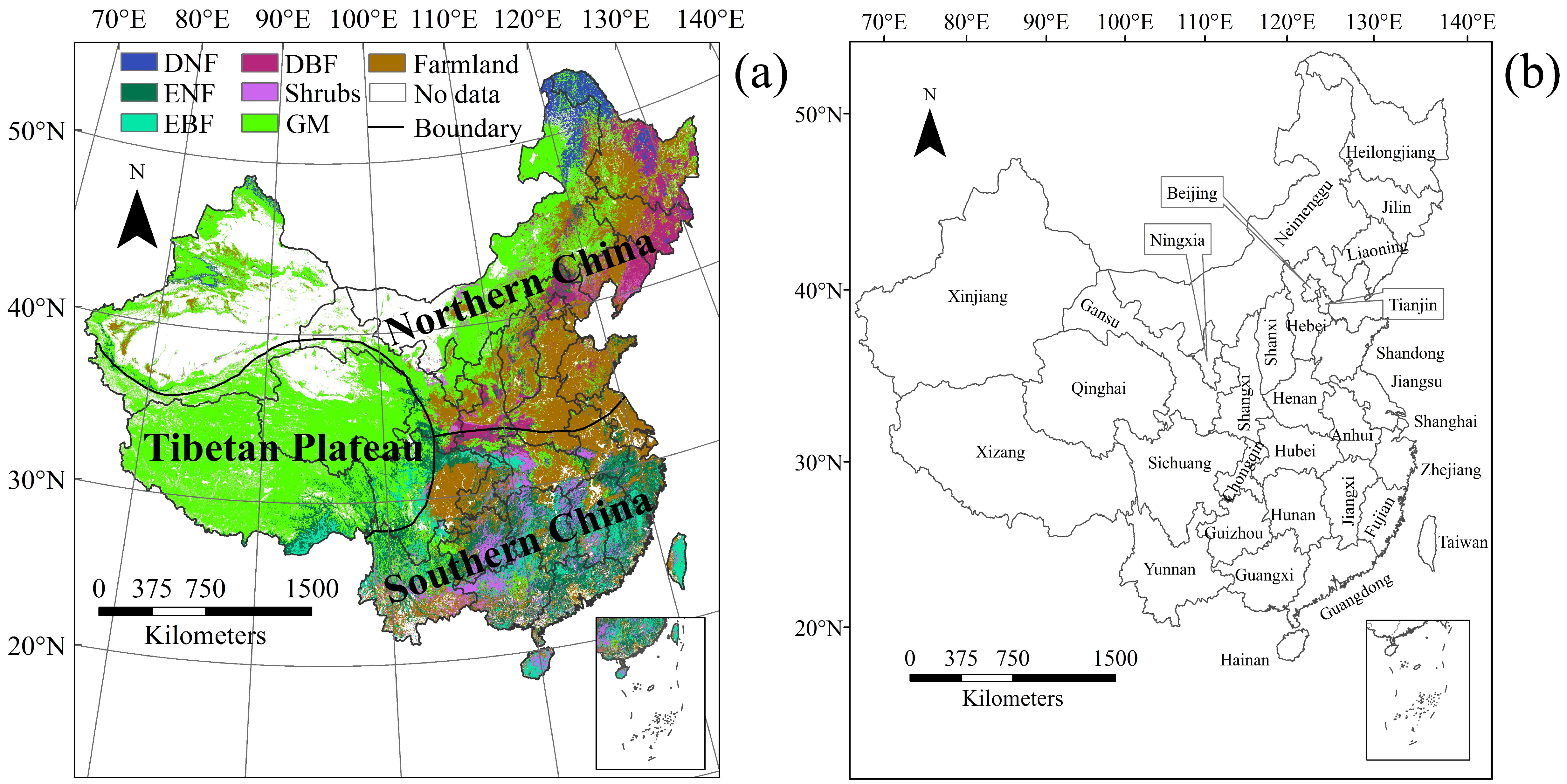
2.1. Study Area

China is situated within the world’s largest continental landmass (Eurasia), is adjacent to the world’s largest body of water (the Pacific Ocean), and encompasses the world’s highest and largest plateau (the Tibetan Plateau). As such, the location and topography of China is complex, with climatic zones ranging from the tropical southern regions to cold temperate northern regions and the frigid Tibetan Plateau. Accordingly, we divided China into three sub-regions (Figure 1a) based on climatic regionalization [29]: Northern China, with mean annual temperatures ranging from −4 °C to 14 °C and total annual precipitation ranging from 200 mm in the northwest to 1000 mm in the southeast; Southern China, with mean annual temperatures between 14 °C and 22 °C and total annual precipitation ranging from 1000 mm to 2000 mm [28]; and the Tibetan Plateau with an average altitude close to 4000 m a.s.l. (Figure S1) and mean annual temperatures and mean annual precipitation ranging from −5 °C to 12 °C and more than 800 mm to less than 200 mm, respectively [25].

2.2. Data Source and Data Processing

2.2.1. MODIS EVI Data

The MODIS enhanced vegetation index (EVI; MOD13A2) product incorporates enhanced atmospheric correction, cloud detection, and improved geo-referencing as well as an enhanced ability to monitor vegetation [30]. It was developed to: (1) enhance the vegetation signal with improved sensitivity in high biomass regions; (2) minimize the impacts of canopy background variation while retaining sensitivity to small changes in vegetation activities [31]; and (3) reduce the impact of smoke from biomass burning in tropical areas [32]. This index has been suggested to be more appropriate for monitoring vegetation dynamics that are covered even by sparse vegetation [31] and has been applied as an appropriate dataset for studying land surface phenology in both temperate and tropical zones [18,33]. Furthermore, the data are processed using the maximum value composite (MVC) method to reduce cloud, atmosphere, sensor, and surface bidirectional reflectance.

Therefore, MODIS EVI data with a spatial resolution of 1 km and 16-day temporal resolution from 2001 to 2014 were used to estimate land surface phenology in this study. Although the MVC method was used to reduce atmospheric and sensor impacts, the data still contained considerable noise. To obtain more effective time series datasets and to extract accurate land surface phenology, we referenced MODIS quality flag files, replaced ‘VI not produced’ pixels according to the quality flags by using a mean value of adjacent 16-day EVI. If one of the adjacent 16-day EVI was also ‘VI not produced’, we then replaced these pixels with the mean value of the adjacent two years EVI value [34], and excluded pixels with EVI values less than 0 for each year, and smoothed data (see below for details).

2.2.2. Land Cover Data

The Global Land Cover 2000 (GLC-2000) dataset was used in this study to analyze land surface phenology and its variation across vegetation types. The GLC-2000 land cover dataset was independent from the MODIS dataset. Since MODIS land cover data was calculated with MODIS EVI, it could be less independent when analyzing them together. The GLC-2000 dataset created by daily S1 data acquired from the VEGETATION sensor on board the SPOT-4 satellite. This dataset was generated using different classification methods, and it takes local expert knowledge into consideration to improve data accuracy relative to similar datasets [35]. The GLC-2000 land cover classes were further reclassified into 7 major land cover classes (Figure 1a) in the present study: deciduous needle-leaf forest (DNF), evergreen needle-leaf forest (ENF), evergreen broadleaf forest (EBF), deciduous broadleaf forest (DBF), grassland and meadow (GM), shrubs, and farmland (Figure 1a). These categories only reflect the land cover classification and do not consider changes in land cover that occurred during our study period. While changes in these classifications are likely to have occurred (Table S1), we assumed that their overall effects on forest ecosystems were negligible in the context and scope of this work during the study period, because the spatial and temporal patterns of land cover, especially for vegetation, might be relatively stable over short time periods of approximately 10 years at regional or global scales [36].

2.2.3. Data Smoothing and Phenology Extraction

The original synthesized EVI time-series data contained singular values that would affect dataset precision and impose substantial limitations [13]. However, currently there is not a general method that could be applied universally. Therefore, after preprocessing procedures (i.e., reprojection and image clipping), four methods, namely the Savitzky-Golay method (S-G), the double logistic function method (D-L), the asymmetric Gaussian function method (A-G) and the harmonic analysis of time series method (Hants) were applied to reconstruct EVI time series data (see [37,38,39] for details of the algorithms for the four methods). Then, three statistical indicators, namely the root mean square error (RMSE), Akaike’s Information Criterion (AIC), and Bayesian Information Criterion (BIC) were used to evaluate the performance of each method mentioned above. The three statistical indicators were calculated as follows

$$\mathrm{EMSE}=\sqrt{\frac{{\sum }_{i=1}^N{\left(EV{I}^{*}\left(t\right)-EVI\left(t\right)\right)}^2}{N}}$$

(1)

$$\mathrm{AIC}=2k+N\times \ln \left(RSS\right)$$

(2)

$$\mathrm{BIC}=N\times \ln \left(RSS\right)+k\times \ln \left(N\right)$$

(3)

where EVI^*(t) is the smoothing result of EVI, EVI(t) is the mean EVI value obtained from the four methods (assumed to be accurate), N is the number of time points, k is the number of free parameters (k = 2, 6, 7, and 5 for S-G, D-L, A-G and Hants, respectively), and RSS is the residual sum of squares between mean EVI and the corresponding smoothing methods. Lower values of RMSE, AIC, and BIC indicate a preferable method.

Our result (Table S2) indicated that the S-G method was the best of the four. The S-G filter is computed as follows:

$$Y_j^{*}=\frac{{\sum }_{i=-m}^{i=m}{C}_i\times Y_{j+1}}{N}$$

(4)

where Y is the original EVI value, $Y^{*}$ is the resultant EVI value, $C_i$ is the coefficient for the ith EVI of the smoothing window, N is the number of convoluting integers and is equal to the smoothing window size (2m + 1), j represents the running index of the ordinate data in the original data table, and m represents the half-width of the smooth window.

Then, we used TIMESAT software, which is widely used for estimating land surface phenology [18,19,36,40], applying the S-G method to generate smooth time-series EVI data. We adopted the adaptation strength of 2.0, no spike filtering, seasonal parameter of 0.5, S-G window size of 2, and amplitude season start and end of 20% to calculate the phenology parameters. We calculated land surface phenology (SOS and EOS for each year) and obtained LOS as the difference between SOS and EOS values.

2.3. Data Analyses

2.3.1. Mann-Kendall Trend Analysis

The trend of phenological metrics during 2001–2014 was calculated at a pixel level and regional level; however, a certain degree of autocorrelation may exist in these inter-annual time series data; therefore, in this study, a robust non-parametric Mann-Kendall (M-K) trend analysis was applied because it does not require the independence and normality of the time series data [16]. It has been reported that the M-K test statistic Z is approximately normally distributed when the sample size n ≥ 8 [41]. A positive and a negative Z value, respectively, indicate an increasing and a decreasing trend. It should be noted that the M-K procedure is a test for the presence of a monotonic trend and not a strictly linear trend [41]. M-K in this study was calculated as follows (see [42] for details):

$$\mathrm{S}={\displaystyle \sum }_{i=1}^{n-1}{\displaystyle \sum }_{j=i+1}^{n}sgn\left(x_j-x_i\right)$$

(5)

where n is the number of data points, $x_i$ and $x_j$ are the data values at times i and j (j > i), respectively, and $sgn\left(x_j-x_i\right)$ is the sign function

$$sgn\left(x_j-x_i\right)=\{\begin{array}{c}+1,if{x}_j-x_i>0\\ 0,if{x}_j-x_i=0\\ -1,if{x}_j-x_i<0\end{array}$$

(6)

The variance is calculated as

$$Var\left(\mathrm{S}\right)=\frac{n\left(n-1\right)\left(2n+5\right)-{\sum }_{i=1}^m{t}_i\left(t_i-1\right)\left(2t_i+5\right)}{18}$$

(7)

where n is the number of data points, m is the number of tied groups and $t_i$ denotes the number of ties of extent i. A tied group is a set of sample data that have the same value.

The test statistic Z is calculated using Equation (8). Trends were tested at specific α significance level, and in this study, α = 0.05 was used.

$$\mathrm{Z}=\{\begin{array}{c}\frac{S-1}{\sqrt{Var\left(s\right)}},ifS>0\\ 0,ifS=0\\ \frac{S+1}{\sqrt{Var\left(s\right)}},ifS<0\end{array}$$

(8)

2.3.2. Theil–Sen Median Slope Estimator

The Theil–Sen median slope estimator was applied to estimate the rate of change of phenological metrics, which is more appropriate for assessing the rate of change in short or noisy time series [43]. The Theil–Sen median slope was computed as

$${\beta }_i=\mathrm{Median}\left(\frac{x_j-x_k}{j-k}\right)\mathrm{for}i=1,\dots ,N$$

(9)

where $x_j$ and $x_k$ are the data values at times j and k (j > k), respectively.

All the analyses were conducted in ARCGIS 9.3 (ESRI, Redlands, CA, USA), ENVI 5.1 (Exelis Visual Information Solutions, Boulder, CO, USA), and MATLAB R2014a (The Mathworks, Inc., Natick, MA, USA).

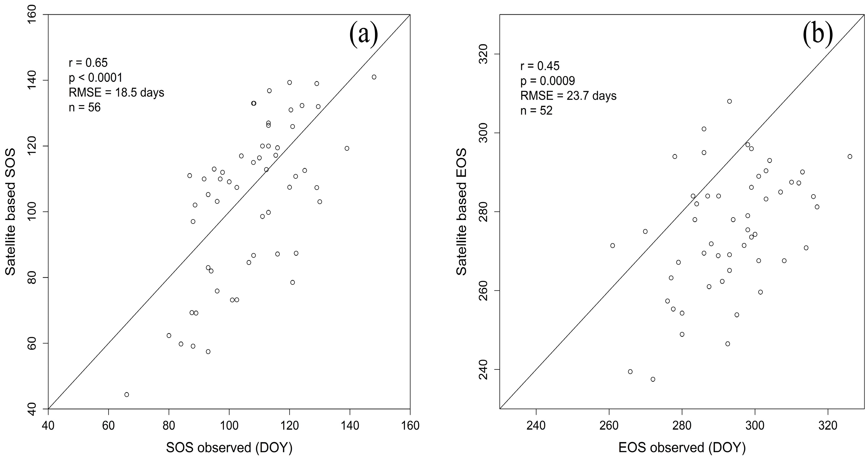
2.4. SOS and EOS Validation

We evaluated our results (for SOS and EOS) via ground observations (from 56 sites for SOS data and 52 sites for EOS data) of previously published studies encompassing the time range between 2000 and 2014 (Table S3). Similar to the method used by Liang et al. [44], we utilized MOD09A1 data to acquire ‘pure’ endmember signatures to apply the linear spectral unmixing method. Then, the SOS and EOS values were weighted as the corresponding proportion. Finally, the root mean square error (RMSE) and correlation coefficient (r) between estimated and field-observed SOS and EOS values were calculated.

3. Results

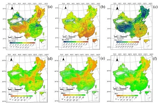
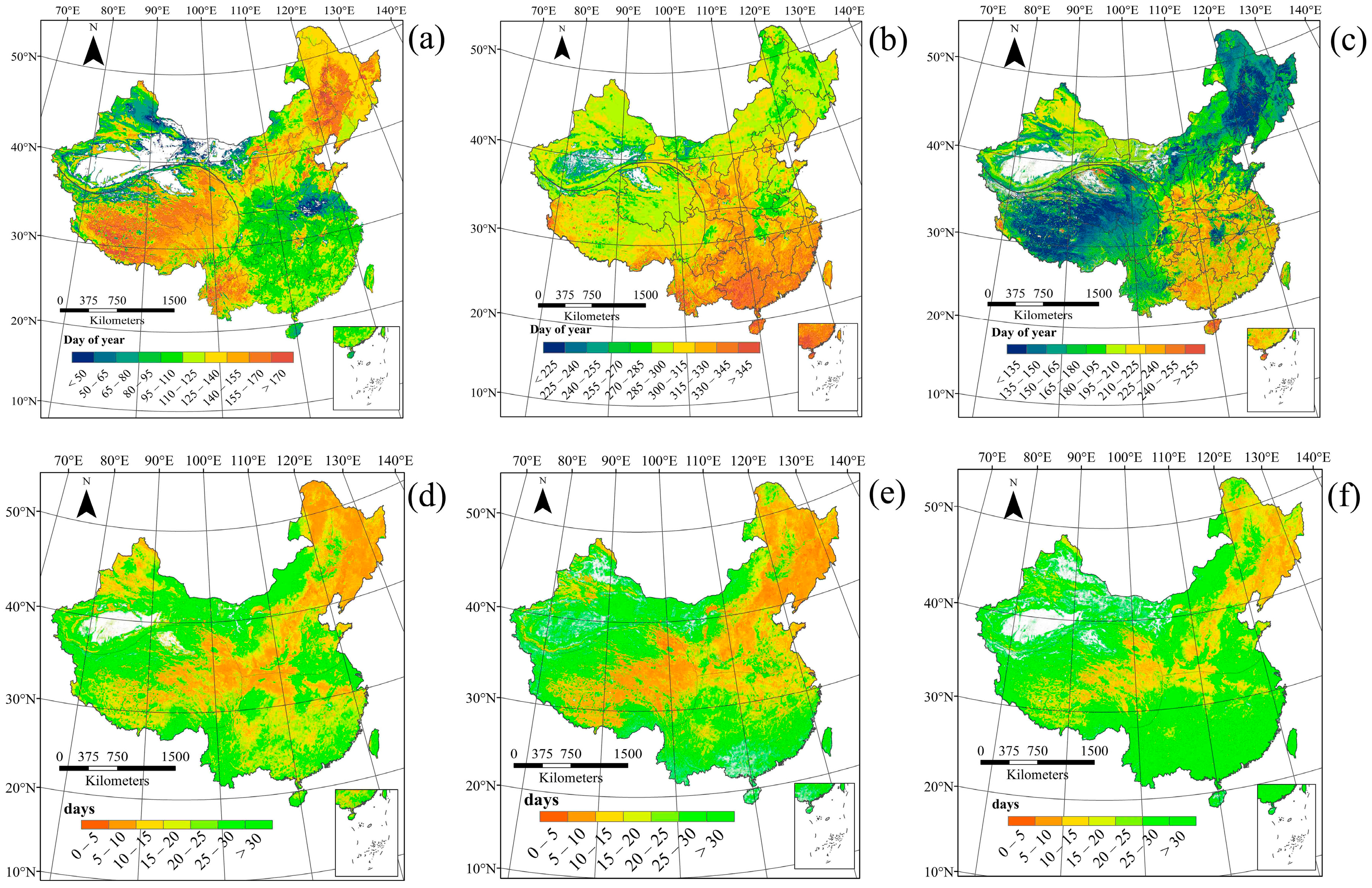
3.1. Spatial Patterns of Land Surface Phenology

The mean phenological parameter data were calculated on a pixel scale over the study period (2001–2014). The spatial distribution of phenology exhibited apparent variability across the study area (Figure 1b and Figure 2). SOS (Figure 1b and Figure 2a) was mainly distributed in the range of days 65–170 of the year (65–170 DOY) and was progressively delayed with increasing latitude and altitude. An early SOS before 65 DOY mainly occurred within Hainan province, the North China Plain, and desert areas. A later SOS, occurring at 125–170 DOY, was mostly distributed within northeastern China as well as the middle and eastern Tibetan Plateau. Regions with SOS after 170 DOY were found in east Inner Mongolia as well as the southwestern Tibetan Plateau. For other regions, SOS generally fell between 65 and 125 DOY. Compared with SOS, EOS exhibited an opposite trend in its spatial distribution (Figure 1b and Figure 2b); in other words, EOS was delayed with increasing latitude and altitude. The earliest EOS values mostly occurred around desert areas (earlier than 225 DOY), whereas the latest EOS values, occurring after 300 DOY, were mainly found below 30°N. EOS ranging from 255 to 300 DOY were mainly distributed between 30°N and 40°N, while some regions did not conform to this pattern; for instance, EOS in Beijing, Tianjin, and Shanghai occurred at 315–330 DOY. EOS in the northwest Tibetan Plateau, north Anhui Province, and east Henan province mainly occurred before 300 DOY. Other regions, for instance, northeastern China, east Inner Mongolia, and the western Xinjiang province, exhibited EOS generally within the range of 285–300 days. LOS mostly varied from 135 to 240 days and showed clear spatial patterns over this region that decreased from south to north and from east to west (Figure 2c). The longest LOS, of more than 210 days, occurred in Southern China. In contrast, the shortest LOS, of less than 150 days, was mainly distributed in the Tibetan Plateau and the northeast China Plain. LOS ranged from 150 to 195 days most often in the western Xinjiang Province and Inner Mongolia.

To validate our findings, we compared our results with ground observations (Figure 3). Significant correlations were identified between ground observed phenology and satellite based data, with significant correlation coefficients of 0.65 and 0.45 (both p < 0.001) for SOS and EOS, respectively. The corresponding RMSEs were 18.5 and 23.7 days, respectively.

3.2. Trends in Phenology

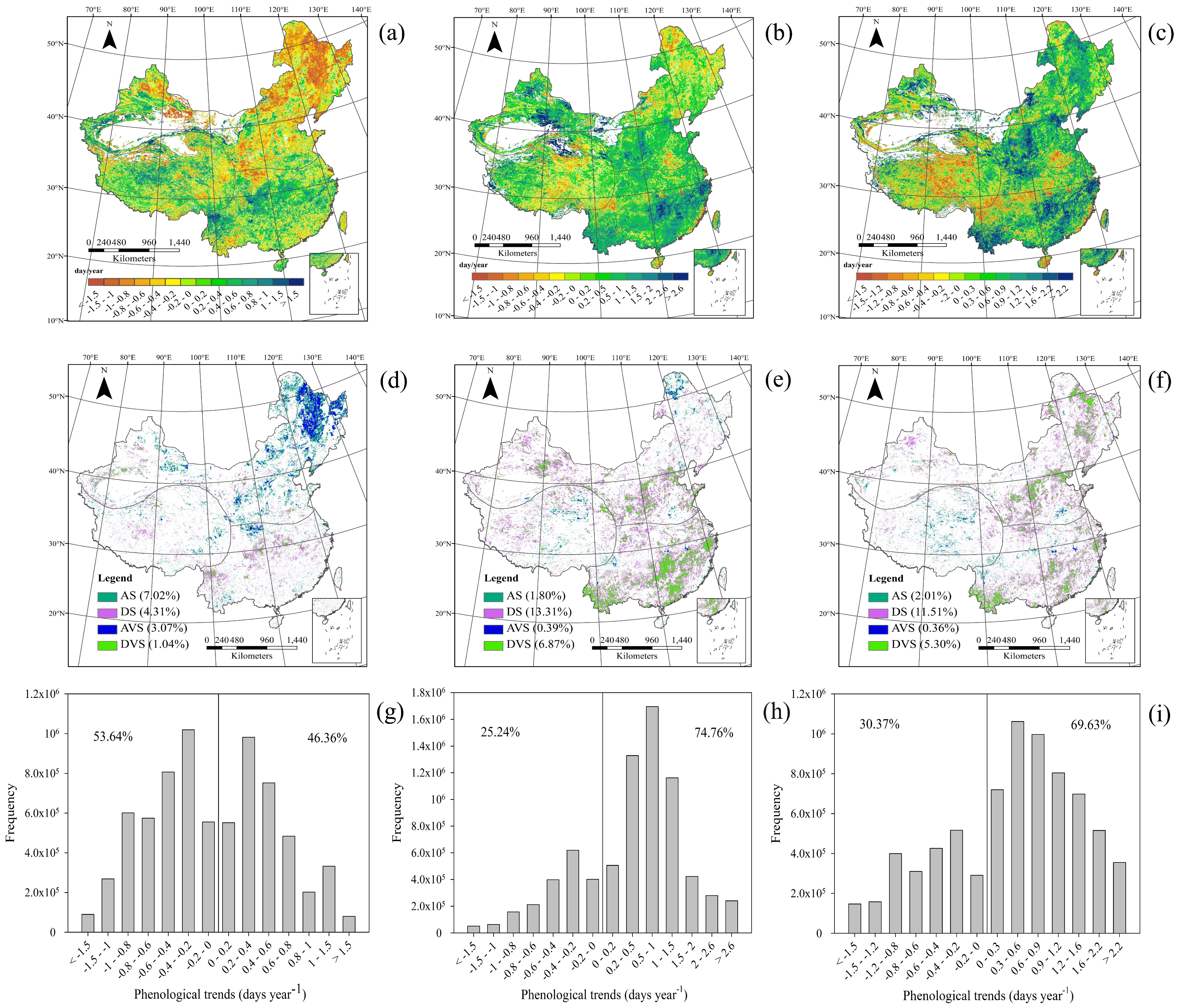
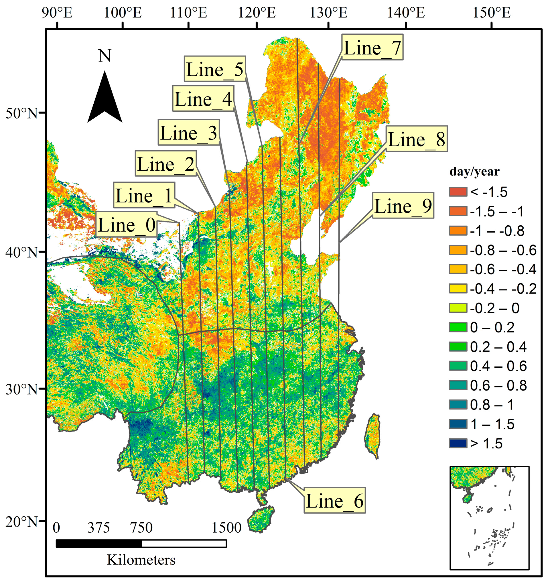
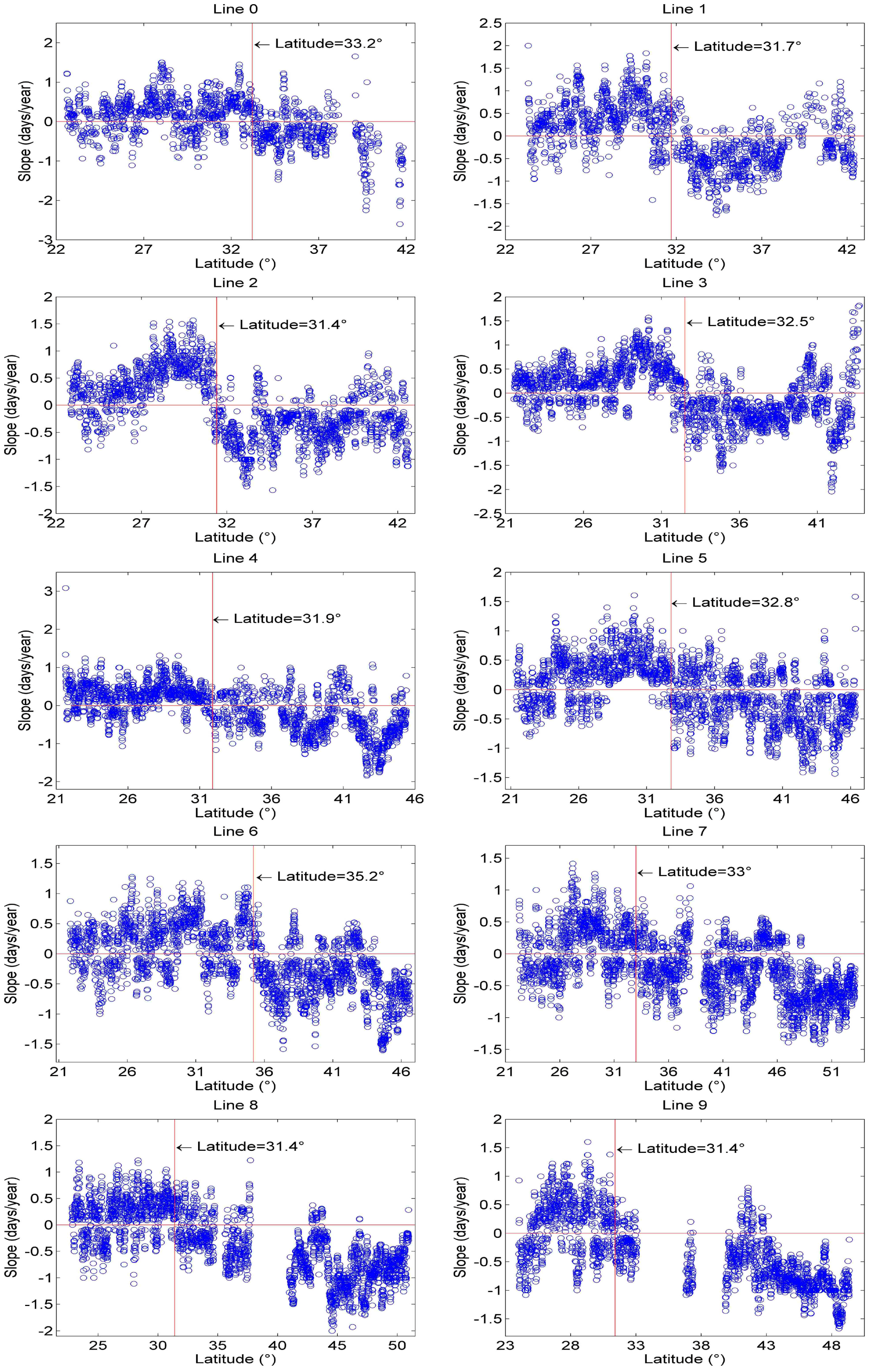
3.2.1. Spatial Patterns of Phenological Trends

Figure 4 shows the spatial patterns and trends in SOS, EOS, and LOS across China. Over 14 years (2001–2014) in the whole study region, 15.44% of total pixels displayed either significantly early onset or delayed trends (Figure 4d; p < 0.05). Pixels with a negative (i.e., early onset) trend in SOS accounted for 53.64% of the total pixels and 10.09% of the total pixels exhibited a significantly negative trend (Figure 3g; p < 0.05). Negative SOS trends mainly occurred in northeastern China and Inner Mongolia, whereas pixels with positive (i.e., delayed) trends mainly occurred below 35°N and in the western Xinjiang province (Figure 4a). The absolute values of negative and positive trends in SOS were mainly between 0.2 and 0.6 days/year (Figure 4g).

In contrast to SOS, 22.37% of pixels over the entire study area exhibited EOS values with significant changes (Figure 4e; p < 0.05). Pixels with a delayed EOS trend accounted for 74.76% of the total, and 20.18% of the total pixels exhibited a significant positive (i.e., delayed) trend (Figure 4e,h; p < 0.05). Delayed EOS mainly occurred in Southern China, the North China Plain, and in Xinjiang province, while the EOS exhibited an early onset trend mainly distributed across the middle of the Tibetan Plateau, north of 50°N, and in eastern Inner Mongolia (Figure 4b). The magnitude of delayed and early onset trends for EOS was mainly between 0.2 and 1.5 days/year, and no more than −0.8 days/year, respectively.

Over the entire study area, 19.18% of the pixels exhibited significant changes in LOS (Figure 4f; p < 0.05). Extended LOS occurred within 69.63% of all pixels (Figure 4i), with 16.81% pixels exhibiting significant extensions of LOS (Figure 4f; p < 0.05), mostly distributed across northern China and southeast China (Figure 4c). In contrast, decreasing LOS trends occurred in 30.37% of pixels, which were mainly distributed across the central Tibetan Plateau (Figure 4c,i).

3.2.2. Temporal Patterns of Phenological Trends

To clarify the characteristics of phenological trends, averaged trends of phenological metrics at national level and regional level (in Northern China, Southern China, and the Tibetan Plateau) were calculated over the past 14 years (

Table 1. Inter-annual variation of area-averaged start of season (SOS), end of season (EOS), and length of season (LOS) between 2001 and 2014.

Area	Phenology Metrics	Z Test Statistic	p Value	Slope
China	SOS	−0.7664	0.2217	−0.0892
	EOS	2.6278	0.0043	0.2878
	LOS	2.5183	0.0059	0.3604
Northern China	SOS	−2.4088	0.0080	−0.3434
	EOS	1.8613	0.0314	0.1986
	LOS	2.1898	0.0143	0.4595
Tibetan Plateau	SOS	1.5329	0.0627	0.3354
	EOS	0.7664	0.2217	0.2023
	LOS	−0.9854	0.1622	−0.1950
Southern China	SOS	1.6423	0.0503	0.2475
	EOS	3.0657	0.0011	0.7852
	LOS	2.7372	0.0031	0.6630

Yearly mean phenology values were calculated using all pixels for the above four study areas.

). No statistically significant early onset trend for SOS in China was observed through the entire study period (slope = −0.09, p = 0.22); however, EOS and LOS were all significantly delayed or extended by 0.29 days/year and 0.36 days/year (all p < 0.01), respectively. Northern China exhibited similar trends as those occurring at the national scale; SOS significantly advanced by 0.34 days/year (p < 0.01), EOS and LOS were significantly delayed and/or extended by 0.20 days/year and by 0.46 days/year (all p < 0.05), respectively. In contrast, SOS in the Tibetan Plateau and Southern China exhibited marginally significant (p < 0.1) trends of 0.34 days/year and 0.25 days/year, respectively. In addition, LOS exhibited contrary trends between the Tibetan Plateau and Southern China with a non-significant shortening of 0.20 days/year (p = 0.16) and a significant extension of 0.66 days/year (p < 0.01), respectively. The EOS trend within the Tibetan Plateau and Southern China were the same as those exhibited across the entire study area, with delays of 0.20 days/year (p = 0.22) and 0.79 days/year (p < 0.01), respectively.

3.2.3. Phenological Trends for Vegetation Types

The trend in phenophases for the period between 2001 and 2014 was calculated for the different vegetation types over the entire study area (

Table 2. Inter-annual variation in phenological metrics [start of season (SOS), end of season (EOS), and length of season (LOS)] for each of the different vegetation types from 2001 to 2014 in China.

		DBF	DNF	EBF	ENF	Farmland	Shrub	Grassland
SOS	Z	−2.1898	−1.4234	1.9708	2.5183	−1.4234	0.8759	0.0000
	p value	0.0143	0.0773	0.0244	0.0059	0.0773	0.1905	0.5000
	slope	−0.2954	−0.4313	0.2662	0.2662	−0.1587	0.1217	0.0159
EOS	Z	1.6423	−0.7664	2.6278	3.3942	2.9562	2.6278	1.0949
	p value	0.0503	0.2217	0.0043	0.0003	0.0016	0.0043	0.1368
	slope	0.3115	−0.1836	0.7194	0.7017	0.4776	0.7003	0.1839
LOS	Z	2.6278	0.5474	2.6278	2.9562	3.1752	2.9562	0.5474
	p value	0.0043	0.2921	0.0043	0.0016	0.0007	0.0016	0.2921
	slope	0.5721	0.1953	0.5887	0.5817	0.4853	0.4987	0.1503

DBF, deciduous broadleaf forests; DNF, deciduous needle leaf forests; EBF, evergreen broadleaf forests; ENF, evergreen needle leaf forests; GM, grassland and meadow.

). During that period, the trends in SOS, EOS, and LOS showed substantially different characteristics according to each vegetation type. For DBF, EBF, and ENF vegetation types, SOS exhibited significantly early onset or delays over the past 14 years, and the early onset or delay of SOS in DBF, EBF, and ENF were −0.30 days/year (p < 0.05), 0.27 days/year (p < 0.05), and 0.27 days/year (p < 0.01), respectively. No significant trend in SOS was observed for other vegetation types at a 95% confidence level.

All vegetation types exhibited a delayed EOS trend over the 14 years except the DNF vegetation type, which showed a non-significant early onset of −0.18 days/year (p = 0.22). Among all delayed EOS vegetation types, significance at a 95% confidence level was observed except for DBF and GM vegetation types (p = 0.05 and p = 0.14, respectively). The strongest trend occurred in EBF and ENF vegetation types, the magnitudes of these trends were 0.72 days/year (p < 0.01), and 0.70 days/year (p < 0.001), respectively.

Different vegetation types displayed extended LOS to varying degrees over the past 14 years (Table 2). The trend in extended LOS was very significant (p < 0.01) for all vegetation types except DNF and GM (all p = 0.29). For DBF, EBF, ENF, farmland, and shrubs, LOS was extended by about 0.57, 0.59, 0.58, 0.49, and 0.50 days/year, respectively (all p < 0.01).

4. Discussion

4.1. Spatial Distribution in Phenology Parameters

An examination of the variability in land surface phenology of China over the last 14 years reveals substantial spatial variation in SOS, EOS and LOS. Generally, the average SOS was delayed with latitude or altitude. Interestingly, SOS in Yunnan province was later than in surrounding regions due to its relatively high altitude (an average altitude of 2000 m a.s.l.), which typically results in lower temperatures. A similar situation was observed in northeastern China as a result of its vegetation type (soybean and spring wheat), which may be mostly affected by sowing date, irrigation, and fertilizer application; an early SOS date occurring in the middle to lower delta of the Yangtze River supports this point of view (Figure 1b and Figure 2a). In addition, we found SOS in east Guangxi, Guangdong, and Fujian mainly occurring in April, which was in line with the findings of Qiu et al. [27]; this is likely a result of plant leaves in those areas falling from January to March and new leaves emerging in late March and April. In contrast to SOS, EOS displayed early onset trends associated with latitude or altitude increases. In addition, EOS of cropland was earlier than in surrounding areas with other plant types due to human activities such as harvest date. LOS shortened with latitude or altitude increases. Our results are supported by previous studies [12,17,20,45,46]. Although our findings regarding Southern China were supported by Qiu et al. [27], there are few recent studies that discuss the concrete dates of phenology parameters within that region to the best of our knowledge. This is likely due to the indistinguishable seasonality and/or complex ecosystems of the region, which makes it difficult to conduct these studies except on a hemispheric or global scale [13,47].

We validated our results with ground-based measurements, and it is noteworthy that the SOS estimates obtained from remote sensing tended to be somewhat later than those from field observation, concurring with Suepa et al. [18], while EOS exhibited the opposite bias. This is because remote sensing captures vegetation canopy ‘greenness’ unlike field observations, which are directly based on individual plants that using specific and somewhat subjective measures like 50% leaf emergence thresholds. Similarly, EOS extracted from remote sensing may therefore be more related to leaf coloration than to actual leaf fall [33]. In addition, field observations are usually tracked through seasonal development milestones (i.e., budburst, leaf-out, leaf coloration changes, and leaf fall). In contrast, remote sensing methods capture land surface phenology and primarily track correlates of leaf chlorophyll content and structure [48] at a scale affected by composite factors (e.g., complex surface reflectance). Thus, remote-sensing methods describe of vegetation canopy greenness (spatially and species-aggregated) that integrates complex signals (i.e., vegetation greenness, vegetation cover, related reflectance, and land surface processes; [49]). Therefore, remote-sensing methods offer estimates of qualitatively different traits that cannot precisely correspond with ground-based measurements [9].

Although there are some mismatches between remote sensing dates and field-observed dates, field observations appear to be the best available data for validating remote sensing data currently and phenology parameters obtained from remote sensing remain useful for large spatial and longer temporal studies for which field observational date are currently meager or lacking, especially in Southern China and the Tibetan Plateau. This is important both in terms of spatial coverage and temporal coverage. Accordingly, it is better to compare satellite measures with ground-based data at commensurate spatial scales and continuously. This should be conducted along with a substantial upscaling of intensive and broad ground measurements over continuous geographic coverages in order to bridge the gap between ground observations and satellite-derived measurements. This may help remedy inaccuracies in interpreting satellite-derived measurements.

Unlike many other studies, we included analyses of cropland, which was usually excluded by past studies [12,20,21,50] due to the obvious influence of human activities. Lu et al. [51] found that the SOS of winter wheat in North China mainly occurred at 60–150 DOY. Wu et al. [48] showed that SOS occurred in early March to late April in most croplands, such as the North China Plain and the plain within the middle delta of the Yangtze River, while SOS in northeast China normally occurs from early May to late June. EOS of most single-crop farmland often occurred from September to October. Although our results were consistent with those studies, our results could not fully capture cropland phenology, which is characterized by a second growing season in some areas of China. However, when we compared our results with those of Xiao et al. [52], who based their conclusions on field observations, the trends in both SOS and EOS determined by the present study were the same as those identified by Xiao et al. [52] for most stations. This suggests that even though some errors might be associated with remote-sensing data, the trend we inferred in crop phenology is still reliable. Indeed, there is no definite relationship between field observations and corresponding remote-sensing data for cropland due to the different observation contents, scales, and criteria. Therefore, to improve the reliability of remote-sensing data, it is appropriate to compare trends over time or time ranges rather than comparing specific dates obtained with these methods. In addition, the validation based on extensive field observations and high spatial resolution images in the future would enable excellent results when the method provided by Liang et al. [44] is taken into account, particularly for mixed pixels.

4.2. Temporal Changes in Phenology at the Regional Scale

The phenological trends at a national scale were in accordance with previous findings [26,47]. Interestingly, we found that the magnitude of changes in SOS over the last two decades of the twentieth century (as shown in previous studies) exceeded those inferred with data generated after 2000 (i.e., in this study); this finding appears to support the main result of previous studies [9,13,47,53,54] that the change rate of SOS has decreased due to a deceleration of strong warming in recent decades [55], or changes in winter chilling or fire regimes at a regional scale [47,54].

The trends were heterogeneous in both direction and magnitude at the regional scale across the study period. The magnitude of SOS in Northern China was less than that estimated by Chen et al. [56], Gong et al. [17], and Piao et al. [45], but slightly higher than the estimate obtained by Cong et al. [19] and Ge et al. [10]. Relative to SOS, the magnitude of EOS was similar to that of Ge et al. [10], but slightly higher than that of Yang et al [50].

The discrepancy in phenological trends and corresponding magnitudes across studies may be caused by differences in study area, study period, and/or study methods. For example, Gong et al. [17] only assessed Inner Mongolia and Cong et al. [19] studied temperate China, including most of the Tibetan Plateau. These large-scale study areas have different vegetation types, water availability, heat conditions, and climatic zones, thus impacting overall trend magnitude estimates. In addition, study periods can also affect results [36] because land surface phenology changes with climatic factors (i.e., temperature and precipitation) and land use (i.e., vegetation type and land management). For instance, Yang et al. [50] and Liu et al. [33] illustrated that the EOS trend in temperate China was a delay of 0.13 days/year from 1982 to 2010 and 0.12 days/year from 1982 to 2011, which was much less than the estimate by Piao et al. (0.37 days/year from 1982 to 1998 in temperate China) [44]. Zhu et al. [36] illustrated that the SOS trends in North America were −0.273, −0.349, and −0.132 days/year, while EOS trends were 0.782, 0.420 and 0.551 days/year from 1982 to 1991, 1982 to 1999, and 1982 to 2006, respectively. Moreover, the magnitude of satellite-derived phenological trends differed among methods [9], providing complementary but qualitatively different information [49]. For instance, the SOS in North America was estimated to exhibit delaying trends of 0.03 and 0.13 days/year using the TIMESAT method [34] and Piecewise logistic method [36], respectively. Estimates in temperate China ranged from −0.01 to −0.19 days/year across five different methods [19]. This confirms that there are relatively large uncertainties consistent with the noise in vegetation index (VI) time-series data as well as a substantial influence in setting critical thresholds for onset data [19,21]. Hence, it is critical to choose an appropriate method for a specific region, especially for vast areas with diverse vegetation types and/or harsh environments [21]. Moreover, the merits and defects of smoothing processes in the context of different methods require more in-depth discussion.

The trends in EOS and LOS in the Tibetan Plateau were consistent with previous results [23]. Relative to EOS and LOS, Ding et al. [53] demonstrated that SOS in the Tibetan Plateau showed a non-significant delayed trend from 1999 to 2006 and from 1999 to 2012 using four different methods; the present study was consistent with their results and was also supported by previous studies [23,46]. The delayed trend may be the product of increasingly severe aridity, unmet chilling or photoperiod requirements for plants [57], and a cooling trend in spring air temperatures [23]. Some studies have reported that SOS has continuously occurred earlier in the Tibetan Plateau [58]; the discrepancies among results may be the product of differences in vegetation index responses to vegetation growth between sensors [59] and/or measurements for estimating phenology. Furthermore, SOS trends in the Tibetan Plateau may vary with longitude [16] and elevation [23] due to variation in vegetation types and climate conditions; thus, the considerable spatial heterogeneity of the Tibetan Plateau may offset the positive and negative change trends observed among pixels [13], and the trend may not be significant or even distinguishable over the entire study area. These results indicate that the SOS trend inferred from remote sensing data across the whole area should be considered with some caution [34]. In addition, ecoregions, climate conditions, elevations, contaminations, grassland degradation, variability in the thawing–freezing process, snow or ice cover, anthropogenic factors, and their combined effects [60,61] should also be taken into consideration when inferring phenological parameters in the Tibetan Plateau in future.

In Southern China, we inferred a delayed or extended temporal trend in SOS, EOS, and LOS. Our results were in accordance with those of Suepa et al. [18] and Zhang et al. [62], both of whom demonstrated that SOS and EOS were delayed in Southeast Asia from 2001 to 2010 and SOS was delayed in tropical climate, regions of Asia from 2000 to 2010, respectively. Similarly, Dash et al. [35] suggested a delayed trend in SOS for evergreen and semi-evergreen forests of India. However, Ma and Zhou [26] showed that SOS occurred 0.40 days/year earlier in tropical and subtropical forests from 1982 to 2006 in China. The discrepancy with the results of Ma and Zhou [26] may have been a product of their relatively long study period that may include a potential turning point that offsets the entire trend over the whole study period [12]. Interestingly, SOS in Northern China and Southern China exhibited contrary trends and were separated by a transition zone between approximately 31°N and 35°N (Figure 4a). To precisely characterize the transition zone, we acquired mean change rates of 3-pixel wide regions along 10 buffer lines (with a buffer radius of 1 km) in longitudinal dimension (Figure 5) with the Tibetan Plateau excluded and found that the switch occurs between approximately 31.4°N and 35.2°N (Figure 6). This result agrees with findings by Chen et al. [56] and Zhang et al. [63]. The result may be caused mainly by a winter chilling requirement of the flora in Northern China that is far exceeded for vegetation dormancy release due to its high latitude and warming winters having little impact on thermal time requirements. In contrast, the vegetation in Southern China is unable to break its dormancy in the shorted and insufficient cold winter period; thus, the thermal time requirement for SOS has gradually increased in southern regions [64] because of the increasing winter temperature [28]. Alternatively, the flora of Southern China may require a higher threshold temperature to start growth in a warmer environment [46]. Additionally, a delayed SOS trend may result from other factors such as shorter day lengths during an ‘earlier spring’ that counterbalances the effects of higher temperatures [57]. This apparent contrast may be explained by plants in different climatic zones having different responses to chilling and forcing temperature requirements as well as the timing of chilling and forcing periods caused by climate warming [65]. Although few studies have focused on the phenology of evergreen species in tropical and subtropical areas due to their less obvious seasonal variation, changes in ‘greenness’ or ‘senescence’ exhibited by foliage can also be identified by remote sensing from visible changes in canopy biochemistry and the production of new foliage varies seasonally according to canopy species [18]. Therefore, future studies should focus more on variation exhibited by those species.

Notably, land cover that directly affects phenology may be changed by multiple forces such as urbanization and social-economic development; thus, some errors will inevitably be introduced at the pixel or local scale with respect to inferred land surface phenology shifts. However, the spatial and temporal patterns of land cover, especially for vegetation, might be relatively stable over a short time period of approximately 10 years at regional or global scales [36]. Therefore, the spatial and temporal patterns of land surface phenology inferred in our study may still be reasonable during 2001–2014 in China.

4.3. Temporal Changes in Phenology among Vegetation Types

Analyzing the changes in phenology for different vegetation types can reveal the hydrothermal effects acting in different areas. Previous studies have shown that the trends and magnitude of SOS were non-significant despite considerable differences among vegetation types [13]. Consistent with previous studies, we found that trends in SOS among different vegetation types without marked or consistent early onset or delays during the study period (ranging from −0.43 to 0.27 days/year; Table 2). Although the absolute magnitudes of SOS for woody vegetation were higher than those estimated for herbaceous vegetation, the magnitudes were less than those inferred by Piao et al. [45]. The EOS (except for DNF) and LOS showed consistent delayed and/or extended trends among vegetation types (Table 2). Previous studies have shown that changes in land surface phenology among vegetation types have a wide range of effects on vegetation growth, productivity, competition, and the terrestrial carbon cycle [49]; therefore, it is unclear how much of those functions have changed for an ecosystem regulated by inconsistent trends and magnitude in phenology among different vegetation types. For instance, vegetation productivity and carbon storage may be diminished by delayed SOS; however, it is undetermined if it can be offset by delayed EOS or extend LOS, ultimately resulting in little or no effect on ecosystem function and vice versa. These matters require further research.

Notably, our results showed that the trends in phenological parameters are regionally diverse and species specific, negating our first hypothesis and affirming our second. The discrepancies among phenophases may contribute to the diverse responses and adaptations to climatic factors and spatially uneven changes in climatic variables [20,26]; however, may also result from calculation errors (e.g., from VI smoothing) to some extent.

5. Conclusions

Variation in land surface phenology in China was estimated at national and regional levels during 2001–2014 using MODIS EVI data. Our analyses reveal the following:

(1) Mean SOS was mainly distributed in the range of 65–170 DOY and was delayed as altitude or latitude increases. The mean EOS was mainly between 230 and 310 DOY and exhibited a trend opposite to that of SOS. LOS mostly varied from 135 to 240 days and showed clear spatial patterns over this region, with decreases from south to north and from east to west.

(2) SOS occurred 0.09 days/year earlier at the national level while these trends at the regional level were not uniform. Specifically, SOS in Northern China occurred 0.34 days/year earlier, while the Tibetan Plateau and Southern China exhibited delays in SOS by 0.34 and 0.25 days/year, respectively. In contrast to SOS, EOS exhibited a delayed trend over the study period at both national and regional levels. LOS was extended both at national and regional levels except in the Tibetan Plateau, for which LOS was shortened by 0.20 days/year. In addition, the absolute magnitude of SOS was decreased after 2000 compared with estimates from previous studies.

(3) The trend and magnitude among vegetation types are regionally diverse and species specific. Specifically, SOS did not advance markedly or consistently during the study period, and the magnitudes of SOS changes for woody vegetation were higher than those of herbaceous vegetation. The EOS trends for all vegetation types (except DNF) and LOS trends for all vegetation types showed consistent delays or extensions.

(4) Different SOS trends occurred within Northern China and Southern China, and the transition zone was observed approximately between 31.5°N and 35°N.

References

1. Hmimina, G.; Dufrêne, E.; Pontailler, J.Y.; Delpierre, N.; Aubinet, M.; Caquet, B.; de Grandcourt, A.; Burban, B.; Flechard, C.; Granier, A.; et al. Evaluation of the potential of MODIS satellite data to predict vegetation phenology in different biomes: An investigation using ground-based NDVI measurements. Remote Sens. Environ. 2013, 132, 145–158. [Google Scholar] [CrossRef]
2. Dai, J.H.; Wang, H.J.; Ge, Q.S. The spatial pattern of leaf phenology and its response to climate change in China. Int. J. Biometeorol. 2014, 58, 521–528. [Google Scholar] [CrossRef] [PubMed]
3. Kang, S.Y.; Running, S.W.; Lin, J.H.; Zhao, M.S.; Park, C.-R.; Loehman, R. A regional phenology model for detecting onset of greenness in temperate mixed forests, Korea: An application of MODIS leaf area index. Remote Sens. Environ. 2003, 86, 232–242. [Google Scholar] [CrossRef]
4. Schwartz, M.D.; Carbone, G.J.; Reighard, G.L.; Okie, W.R. Models to predict peach phenology from meteorological variables. HortScience 1997, 32, 213–216. [Google Scholar]
5. White, M.A.; Thornton, P.E.; Running, S.W. A continental phenology model for monitoring vegetation responses to interannual climatic variability. Glob. Biogeochem. Cycles 1997, 11, 217–234. [Google Scholar] [CrossRef]
6. Richardson, A.D.; Jenkins, J.P.; Braswell, B.H.; Hollinger, D.Y.; Ollinger, S.V.; Smith, M.L. Use of digital webcam images to track spring green-up in a deciduous broadleaf forest. Oecologia 2007, 152, 323–334. [Google Scholar] [CrossRef] [PubMed]
7. Sonnentag, O.; Hufkens, K.; Teshera-Sterne, C.; Young, A.M.; Friedl, M.; Braswell, B.H.; Milliman, T.; O’Keefe, J.; Richardson, A.D. Digital repeat photography for phenological research in forest ecosystems. Agric. Meteorol. 2012, 152, 159–177. [Google Scholar] [CrossRef]
8. Henebry, G.M.; de Beurs, K.M. Remote sensing of land surface phenology: A prospectus. In Phenology: An Integrative Environmental Science; Schwartz, M.D., Ed.; Springer: Dordrecht, The Netherlands, 2013; pp. 385–411. [Google Scholar]
9. Fu, Y.S.H.; Piao, S.L.; de Beeck, M.O.; Cong, N.; Zhao, H.F.; Zhang, Y.; Menzel, A.; Janssens, I.A. Recent spring phenology shifts in western Central Europe based on multiscale observations. Glob. Ecol. Biogeogr. 2014, 23, 1255–1263. [Google Scholar] [CrossRef]
10. Ge, Q.S.; Wang, H.J.; Rutishauser, T.; Dai, J.H. Phenological response to climate change in China: A meta-analysis. Glob. Chang. Biol. 2015, 21, 265–274. [Google Scholar] [CrossRef] [PubMed]
11. Rodriguez-Galiano, V.F.; Dash, J.; Atkinson, P.M. Characterising the land surface phenology of Europe using decadal MERIS data. Remote Sens. 2015, 7, 9390–9409. [Google Scholar] [CrossRef]
12. Wu, X.C.; Liu, H.Y. Consistent shifts in spring vegetation green-up date across temperate biomes in China, 1982–2006. Glob. Chang. Biol. 2013, 19, 870–880. [Google Scholar] [CrossRef] [PubMed]
13. Zhao, J.J.; Zhang, H.Y.; Zhang, Z.X.; Guo, X.Y.; Li, X.D.; Chen, C. Spatial and temporal changes in vegetation phenology at middle and high latitudes of the northern hemisphere over the past three decades. Remote Sens. 2015, 7, 10973–10995. [Google Scholar] [CrossRef]
14. Jeganathan, C.; Dash, J.; Atkinson, P.M. Characterising the spatial pattern of phenology for the tropical vegetation of India using multi-temporal MERIS chlorophyll data. Landsc. Ecol. 2010, 25, 1125–1141. [Google Scholar] [CrossRef]
15. Maignan, F.; Bréon, F.M.; Vermote, E.; Ciais, P.; Viovy, N. Mild winter and spring 2007 over western Europe led to a widespread early vegetation onset. Geophys. Res. Lett. 2008. [Google Scholar] [CrossRef]
16. Wang, C.Z.; Guo, H.D.; Zhang, L.; Liu, S.Y.; Qiu, Y.B.; Sun, Z.C. Assessing phenological change and climatic control of alpine grasslands in the Tibetan Plateau with MODIS time series. Int. J. Biometeorol. 2015, 59, 11–23. [Google Scholar] [CrossRef] [PubMed]
17. Gong, Z.; Kawanura, K.; Ishikawa, N.; Goto, M.; Wulan, T.; Alateng, D.; Yin, T. MODIS NDVI and vegetation phenology dynamics in the Inner Mongolia grassland. Solid Earth Discuss. 2015, 7, 2381–2411. [Google Scholar] [CrossRef]
18. Suepa, T.; Qi, J.G.; Lawawirojwong, S.; Messina, P.J. Understanding spatio-temporal variation of vegetation phenology and rainfall seasonality in the monsoon Southeast Asia. Environ. Res. 2016, 147, 621–629. [Google Scholar] [CrossRef] [PubMed]
19. Cong, N.; Wang, T.; Nan, H.J.; Ma, Y.C.; Wang, X.H.; Myneni, R.B. Changes in satellite-derived spring vegetation green-up date and its linkage to climate in China from 1982 to 2010: A multimethod analysis. Glob. Chang. Biol. 2013, 19, 881–891. [Google Scholar] [CrossRef] [PubMed]
20. Liu, Q.; Fu, Y.S.H.; Zeng, Z.Z.; Huang, M.T.; Li, X.R.; Piao, S.L. Temperature, precipitation, and insolation effects on autumn vegetation phenology in temperate China. Glob. Chang. Biol. 2016, 22, 644–655. [Google Scholar] [CrossRef] [PubMed]
21. Cong, N.; Piao, S.L.; Chen, A.P.; Wang, X.H.; Liu, X.; Chen, S.P.; Han, S.J.; Zhou, G.S.; Zhang, X.P. Spring vegetation green-up date in China inferred from SPOT NDVI data: A multiple model analysis. Agric. For. Meteorol. 2012, 165, 104–113. [Google Scholar] [CrossRef]
22. Xu, W.C.; Wang, W.; Ma, J.S.; Yang, X. The characteristics, causes of formation and climatic impact of the 1997–1998 El Niño event. Donghai Mar. Sci. 2004, 22, 1–8, (In Chinese with English Abstract). [Google Scholar]
23. Piao, S.L.; Cui, M.D.; Chen, A.P.; Wang, X.H.; Ciais, P.; Liu, J.; Tang, Y.H. Altitude and temperature dependence of change in the spring vegetation green-up date from 1982 to 2006 in the Qinghai-Xizang Plateau. Agric. For. Meteorol. 2011, 151, 1599–1608. [Google Scholar] [CrossRef]
24. Ge, Q.S.; Dai, J.H.; Cui, H.J.; Wang, H.J. Spatiotemporal variability in start and end of growing season in China related to climate variability. Remote Sens. 2016, 8, 433. [Google Scholar] [CrossRef]
25. Shen, M.G.; Tang, Y.H.; Chen, J.; Zhu, X.L.; Zheng, Y.H. Influences of temperature and precipitation before the growing season on spring phenology in grasslands of the central and eastern Qinghai-Tibetan Plateau. Agric. For. Meteorol. 2011, 151, 1711–1722. [Google Scholar] [CrossRef]
26. Ma, T.; Zhou, C.H. Climate-associated changes in spring plant phenology in China. Int. J. Biometeorol. 2012, 56, 269–275. [Google Scholar] [CrossRef] [PubMed]
27. Qin, B.W.; Zhong, M.; Tang, Z.H.; Chen, C.C. Spatiotemporal variability of vegetation phenology with reference to altitude and climate in the subtropical mountain and hill region, China. Chin. Sci. Bull. 2013, 58, 2883–2892. [Google Scholar]
28. Wang, H.J.; Dai, J.H.; Zheng, J.Y.; Ge, Q.S. Temperature sensitivity of plant phenology in temperate and subtropical regions of China from 1850 to 2009. Int. J. Climatol. 2015, 35, 913–922. [Google Scholar] [CrossRef]
29. Zheng, J.Y.; Yin, Y.H.; Li, B.Y. A new scheme for climate regionalization in China. Acta Geogr. Sin. 2010, 65, 3–12, (In Chinese with English Abstract). [Google Scholar]
30. Justice, C.O.; Vermote, E.; Townshend, J.R.G.; Defries, R.; Roy, D.P.; Hall, D.K.; Salomonson, V.V.; Privette, J.L.; Riggs, G.; Strahler, A.; et al. The Moderate Resolution Imaging Spectroradiometer (MODIS): Land remote sensing for global change research. IEEE Trans. Geosci. Remote Sens. 1998, 36, 1228–1249. [Google Scholar] [CrossRef]
31. Dallimer, M.; Tang, Z.; Bibby, P.R.; Brindley, P.; Gaston, K.J.; Davies, Z.G. Temporal changes in greenspace in a highly urbanized region. Biol. Lett. 2011, 7, 763–766. [Google Scholar] [CrossRef] [PubMed]
32. Huete, A.; Didan, K.; Miura, T.; Rodriguez, E.P.; Gao, X.; Ferreira, L.G. Overview of the radiometric and biophysical performance of the MODIS vegetation indices. Remote Sens. Environ. 2002, 83, 195–213. [Google Scholar] [CrossRef]
33. Liu, L.L.; Liang, L.D.; Schwartz, M.; Donnelly, A.; Wang, Z.S.; Schaal, C.B.; Liu, L.Y. Evaluating the potential of MODIS satellite data to track temporal dynamics of autumn phenology in a temperate mixed forest. Remote Sens. Environ. 2015, 160, 156–165. [Google Scholar] [CrossRef]
34. Zeng, H.Q.; Jia, G.S.; Epstein, H. Recent changes in phenology over the northern high latitudes detected from multi-satellite data. Environ. Res. Lett. 2011. [Google Scholar] [CrossRef]
35. Dash, J.; Jeganathan, C.; Atkinson, P.M. The use of MERIS Terrestrial Chlorophyll Index to study spatio-temporal variation in vegetation phenology over India. Remote Sens. Environ. 2010, 114, 1388–1402. [Google Scholar] [CrossRef]
36. Zhu, W.Q.; Tian, H.Q.; Xu, X.F.; Pan, Y.Z.; Chen, G.S.; Lin, W.P. Extension of the growing season due to delayed autumn over mid and high latitudes in North America during 1982–2006. Glob. Ecol. Biogeogr. 2012, 21, 260–271. [Google Scholar] [CrossRef]
37. Savitzky, A.; Golay, M.J.E. Smoothing and differentiation of data by simplified least squares procedures. Anal. Chem. 1964, 36, 1627–1639. [Google Scholar] [CrossRef]
38. Atkinson, P.M.; Jeganathan, C.; Dash, J.; Atzberger, C. Inter-comparison of four models for smoothing satellite sensor time-series data to estimate vegetation phenology. Remote Sens. Environ. 2012, 123, 400–417. [Google Scholar] [CrossRef]
39. Zhou, J.; Jia, L.; Menenti, M. Reconstruction of global MODIS NDVI time series: Performance of Harmonic Analysis of Time Series (HANTS). Remote Sens. Environ. 2015, 163, 217–228. [Google Scholar] [CrossRef]
40. Jönsson, P.; Eklundh, L. TIMESAT 3.0 Software Manual; Department of Earth and Ecosystem Sciences, Lund University: Lund, Sweden; Center for Technology Studies, Malmö University: Malmö, Sweden, 2010. [Google Scholar]
41. Neeti, N.; Eastman, J.R. A contextual Mann-Kendall approach for the assessment of trend significance in image time series. Trans. GIS 2011, 15, 599–611. [Google Scholar] [CrossRef]
42. Gocic, M.; Trajkovic, S. Analysis of changes in meteorological variables using Mann-Kendall and Sen’s slope estimator statistical tests in Serbia. Glob. Planet. Chang. 2013, 100, 172–182. [Google Scholar] [CrossRef]
43. Zhou, J.H.; Cai, W.T.; Qin, Y.; Lai, L.M.; Guan, T.Y.; Zhang, X.L.; Jiang, L.H.; Du, H.; Yang, D.W.; Cong, Z.T.; et al. Alpine vegetation phenology dynamic over 16 years and its covariation with climate in a semi-arid region of China. Sci. Total Environ. 2016, 572, 119–128. [Google Scholar] [CrossRef] [PubMed]
44. Piao, S.L.; Fang, J.Y.; Zhou, L.M.; Ciais, P.; Zhu, B. Variation in satellite-derive phenology in China’s temperate vegetation. Glob. Chang. Biol. 2006, 12, 672–685. [Google Scholar] [CrossRef]
45. Jin, Z.N.; Zhuang, Q.L.; He, J.S.; Luo, T.X.; Shi, Y. Phenology shift from 1989 to 2008 on the Tibetan Plateau: An analysis with a process-based soil physical model and remote sensing data. Clim. Chang. 2013, 119, 435–449. [Google Scholar] [CrossRef]
46. Jeong, S.J.; Ho, C.H.; Gim, H.J.; Brown, M.E. Phenology shifts at start vs. end of growing season in temperate vegetation over the Northern Hemisphere for the period 1982–2008. Glob. Chang. Biol. 2011, 17, 2385–2399. [Google Scholar] [CrossRef]
47. Yang, Y.T.; Guan, H.D.; Shen, M.G.; Liang, W.; Jiang, L. Changes in autumn vegetation dormancy onset date and the climate controls across temperate ecosystems in China from 1982 to 2010. Glob. Chang. Biol. 2015, 21, 652–665. [Google Scholar] [CrossRef] [PubMed]
48. Lu, L.L.; Wang, C.Z.; Guo, H.D.; Li, Q.T. Detecting winter wheat phenology with SPOT-VEGETATION data in the North China Plain. Geocarto Int. 2014, 29, 244–255. [Google Scholar] [CrossRef]
49. Wu, W.B.; Yang, P.; Tang, H.J.; Zhou, Q.B.; Chen, Z.X.; Shibasaki, R. Characterizing spatial patterns of phenology in cropland of China based on remotely sensed data. Agric. Sci. China 2010, 9, 101–112. [Google Scholar] [CrossRef]
50. Xiao, D.P.; Qi, Y.Q.; Shen, Y.J.; Tao, F.L.; Moiwo, J.P.; Liu, J.F.; Wang, R.W.; Zhang, H.; Liu, F.S. Impact of warming climate and cultivar change on maize phenology in the last three decades in North China Plain. Theor. Appl. Climatol. 2015, 124, 653–661. [Google Scholar] [CrossRef]
51. Liang, L.; Schwartz, M.D.; Fei, S.L. Validating satellite phenology through intensive ground observation and landscape scaling in a mixed seasonal forest. Remote Sens. Environ. 2011, 115, 143–157. [Google Scholar] [CrossRef]
52. Ding, M.J.; Li, L.H.; Zhang, Y.L.; Sun, X.M.; Liu, L.S.; Gao, J.G.; Wang, Z.F.; Li, Y.N. Start of vegetation growing season on the Tibetan Plateau inferred from multiple methods based on GIMMS and SPOT NDVI data. J. Geogr. Sci. 2015, 25, 131–148. [Google Scholar] [CrossRef]
53. Wang, X.H.; Piao, S.L.; Xu, X.T.; Ciais, P.; MacBean, N.; Myneni, R.B.; Li, L. Has the advancing onset of spring vegetation green-up slowed down or changed abruptly over the last three decades? Glob. Ecol. Biogeogr. 2015, 24, 621–631. [Google Scholar] [CrossRef]
54. Guemas, V.; Doblas-Reyes, F.J.; Andreu-Buriollo, I.; Asif, M. Retrospective prediction of the global warming slowdown in the past decade. Nat. Clim. Chang. 2013, 3, 649–653. [Google Scholar] [CrossRef]
55. Chen, X.Q.; Hu, B.; Yu, R. Spatial and temporal variation of phenological growing season and climate change impacts in temperate eastern China. Glob. Chang. Biol. 2005, 11, 1118–1130. [Google Scholar] [CrossRef]
56. Badeck, F.W.; Bondeau, A.; Böttcher, K.; Doktor, D.; Lucht, W.; Schaber, J.; Sitch, S. Responses of spring phenology to climate change. New Phytol. 2004, 162, 295–309. [Google Scholar] [CrossRef]
57. Körner, C.; Basler, D. Phenology under global warming. Science 2010, 327, 1461–1462. [Google Scholar] [CrossRef] [PubMed]
58. Zhang, W.J.; Yi, Y.H.; Kimball, J.S.; Kim, Y.W.; Song, K.C. Climatic controls on spring onset of the Tibetan Plateau grasslands from 1982 to 2008. Remote Sens. 2015, 7, 16607–16622. [Google Scholar] [CrossRef]
59. Shen, M.G.; Zhang, G.X.; Cong, N.; Wang, S.P.; Kong, W.D.; Piao, S.L. Increasing altitudinal gradient of spring vegetation phenology during the last decade on the Qinghai–Tibetan Plateau. Agric. For. Meteorol. 2014, 189, 71–80. [Google Scholar] [CrossRef]
60. Shen, M.G. Spring phenology was not consistently related to winter warming on the Tibetan Plateau. Proc. Natl. Acad. Sci. USA 2011, 108, E91–E92. [Google Scholar] [CrossRef] [PubMed]
61. Yi, S.H.; Zhou, Z.Y. Increasing contamination might have delayed spring phenology on the Tibetan Plateau. Proc. Natl. Acad. Sci. USA 2011, 108, E94. [Google Scholar] [CrossRef] [PubMed]
62. Zhang, X.Y.; Tan, B.; Yu, Y.Y. Interannual variations and trends in global land surface phenology derived from enhanced vegetation index during 1982–2010. Int. J. Biometeorol. 2014, 58, 547–564. [Google Scholar] [CrossRef] [PubMed]
63. Zhang, X.Y.; Tarpley, D.; Sullivan, J.T. Diverse responses of vegetation phenology to a warming climate. Geophys. Res. Lett. 2007. [Google Scholar] [CrossRef]
64. Luedeling, E.; Guo, L.; Dai, J.; Leslie, C.; Blanke, M.M. Differential responses of trees to temperature variation during the chilling and forcing phases. Agric. For. Meteorol. 2013, 181, 33–42. [Google Scholar] [CrossRef]
65. Guo, L.; Dai, J.H.; Wang, M.C.; Xu, J.C.; Luedeling, E. Responses of spring phenology in temperate zone trees to climate warming: A case study of apricot flowering in China. Agric. For. Meteorol. 2015, 201, 1–7. [Google Scholar] [CrossRef]
Figure 1. Vegetation types (DNF, deciduous needle-leaf forest; ENF, evergreen needle-leaf forest; EBF, evergreen broadleaf forest; DBF, deciduous broadleaf forest; and GM, grassland and meadow) across the three sub-region divisions (a) and a map showing provinces of China (b).
Remotesensing 09 00065 g001
Figure 2. Average of start of season (a), end of season (b), and length of season (c) with the corresponding standard deviations within China between 2001 and 2014 (df).
Remotesensing 09 00065 g002
Figure 3. Comparison of the ground-observed start of season (SOS; (a)) and end of season (EOS; (b)) with the corresponding satellite based SOS and EOS values.
Remotesensing 09 00065 g003
Figure 4. Trends in start of season (SOS; (a)), end of season (EOS; (b)), and length of season (LOS; (c)) within China between 2001 and 2014. A positive trend indicates that SOS and EOS were delayed while LOS was extended; in contrast, negative trend indicates that SOS and EOS occurred earlier, while LOS was shortened; individual pixels are shown with significant (p < 0.05) and very significant (p < 0.01) trends for SOS (d), EOS (e), and LOS (f). (DVS, delayed very significantly; DS, delayed significantly; AVS, advanced very significantly; AS, advanced significantly). The count distributions of phenology trends for SOS (g), EOS (h), and LOS (i) are also shown.
Remotesensing 09 00065 g004
Figure 5. Ten lines that were buffered to acquire change rate of SOS during 2001–2014 in China.
Remotesensing 09 00065 g005
Figure 6. Transition zone exhibiting a change in start of season (SOS) in China from 2001 to 2014.
Remotesensing 09 00065 g006