Abstract
The ability of texture models and red-edge to facilitate the detection of subtle structural vegetation traits could aid in discriminating and mapping grass quantity, a challenge that has been longstanding in the management of grasslands in southern Africa. Subsequently, this work sought to explore the robustness of integrating texture metrics and red-edge in predicting the above-ground biomass of grass growing under different levels of mowing and burning in grassland management treatments. Based on the sparse partial least squares regression algorithm, the results of this study showed that red-edge vegetation indices improved above-ground grass biomass from a root mean square error of perdition (RMSEP) of 0.83 kg/m2 to an RMSEP of 0.55 kg/m2. Texture models further improved the accuracy of grass biomass estimation to an RMSEP of 0.35 kg/m2. The combination of texture models and red-edge derivatives (red-edge-derived vegetation indices) resulted in an optimal prediction accuracy of RMSEP 0.2 kg/m2 across all grassland management treatments. These results illustrate the prospect of combining texture metrics with the red-edge in predicting grass biomass across complex grassland management treatments. This offers the detailed spatial information required for grassland policy-making and sustainable grassland management in data-scarce regions such as southern Africa.
1. Introduction
Understanding above-ground grass biomass variations at various scales has become increasingly critical among stakeholders, such as farmers, ecologists and scientists, amongst others. Grasslands are significant carbon sinks, accounting for 18% of the global terrestrial carbon sinks [1]. Furthermore, grasslands are one of the biodiversity hot spots harbouring a wide variety of plants and animals [2], while facilitating soil formation and preservation. From an agricultural perspective, native grasses are the cheapest source of stock feed available. Moreover, grasslands are also a significant source of livelihood, especially to rural communities in southern Africa, where natural disasters and socio-economic hardships are frequent. Collectively, these factors drive the growing interest of accurately monitoring grassland biomass variations for developing optimal management regimes.
A total of 7.5% of the world’s grasslands have been degraded, while about 16% are currently being degraded [3]. Tropical grasslands, specifically, are often at risk of degradation because of increasing pressure from human activities due to population increase [4]. For instance, infrastructural development, crop farming and overgrazing have been cited as the major causes of tropical grassland degradation [3]. Livestock farming has been considered as the fastest growing agricultural sector due to the demand for meat and milk products. Consequently, overstocking and overgrazing have been reported as drivers of grassland degradation. To optimise productivity, while preserving native grasses, numerous grass management practices have been introduced [5]. These include burning, mowing, fertiliser application, as well as controlled grazing [5]. However, insights on the effectiveness of these grass management treatments on grass productivity are limited. This is because there are no cost-effective monitoring systems that have hitherto been developed. Furthermore, the use of existing methods has not been comprehensively evaluated across space and time to the extent that is sufficient for meaningful decision-making and management in data-scarce regions, such as southern Africa.
To acquire comprehensive quantitative information on grass biomass, the utility of earth observation (EO) data has recently become more popular and feasible with an increase, as well as advances, in the available sensors [6]. EO data have been renowned for facilitating rapid, repeated and ongoing biomass observations over various spatial and temporal scales. This is because EO enables comparatively convenient data acquisition dating back over several years, while offering satisfactory ranges of accuracy on above-ground biomass estimation over larger spatial scales. Despite the fact that numerous EO methodologies have been evaluated in quantifying above-ground biomass, no study has hither to illustrate an operational technique that is consistent, precise and repeatable for estimating biomass at local to continental scales. This is caused by the variations in the biophysical, environmental and topographic traits of vegetation in space and time [7,8].
A growing body of literature illustrates that the common approach for estimating biomass, based on EO data, has been to examine the possible association between the ground measured biomass and the EO data, since biomass quantities cannot be directly derived from remotely sensed data [9,10]. Landsat data is the most widely used EO data in vegetation above-ground biomass estimation studies due to its limited costs. However, the majority of the studies have used Landsat for forest inventories [11,12]. The few studies that have been conducted on grass productivity have focused only on a limited number of grass management treatments [13,14].
Furthermore, primary vegetation indices (VIs), such as the normalised difference vegetation index (NDVI), have been widely used for estimating above-ground grass biomass [13,14]. VIs have been widely used because they tend to supersede the influences of the soil background, atmospheric impurities and the viewing and zenith angle effects, while magnifying the signature of vegetation [15,16]. However, these have attained only moderate success in the tropical and subtropical regions [17,18] characterised by complex management treatments, with high spatial heterogeneity. This is due to the lack of strategically located wavebands [19,20], such as the red-edge (i.e., in the Landsat data series). Furthermore, these indices are affected by saturation, soil background and the coarse spatial resolutions for application in grass grown across different grassland management treatments, which still remains a challenge [17,21,22]. This is aggravated by the lack of a clear criterion on the appropriateness of specific EO sensors, proxies, as well as repeatable operational techniques that could provide accurate biomass information from a variety of grass management treatments.
Red-edge (680–740 nm) and texture models seem to offer better proxies, which suppress the soil-background effect, saturation issues [17] and high spatial heterogeneity. Literature shows that the red-edge is sensitive to chlorophyll, as well as leaf structure reflection (i.e., leaf area index, leaf angle distribution), thereby providing more information for the characterization of vegetation [23,24]. More specifically, when the concentration of foliar chlorophyll increases, it results in the bulging of the optical chlorophyll absorption feature, shifting away from the long wavelength margin, and thereby shifting the red-edge to longer wavelengths [25]. Meanwhile, the concentration of leaves of a certain vegetation canopy, as well as the angular nature of those leaves, directly affects the spectral reflectance of that vegetation, especially in the red-edge portion of the electromagnetic spectrum [26]. Subsequently, the biomass of vegetation with a high chlorophyll concentration or leaf area index can then be detected from that with less concentration, based on these shifts. In this regard, it is perceived that the red-edge waveband and its derivatives can better estimate above-ground biomass, when compared to primary bands and vegetation indices [17].
On the other hand, literature indicates that grey level co-occurrence optical texture models also relate better with field measured above-ground vegetation biomass when compared with vegetation indices [7,27]. For instance, work by Cutler et al. [28] indicated that integrating texture metrics data improved biomass estimation from R2 of 0.05, 0.23 and 0.16 to 0.79, 0.79 and 0.84 in Thailand, Malaysia and Brazil, respectively, when compared with multispectral data. Furthermore, texture models offer information that could characterize the subtle structural characteristics of the vegetation canopy, such as those induced by different grassland management treatments. Texture metrics i.e., the grey level co-occurrence matrix, distinguishes minute, but critical, vegetation details, based on a local spectral variation in the image [6]. This is due to the fact that texture models can also suppress the influence of atmospheric effects, the sensor view-angle and the sun view angle, which improve the vegetation spectral signature required for the accurate estimation of above-ground grass biomass [7,29,30]. It is, therefore, important to note that texture variables can optimize the discrimination of vegetation spatial information independently from the tone, while spectral features, i.e., the red-edge, provides detailed vegetation tonal variations that are paramount for accurate vegetation mapping. Based on the above premise, the combination of optimal texture models and red-edge wavebands has a high potential for improving above-ground biomass estimation across different grassland management treatments, superseding the saturation effect of spectral data. To the best of our knowledge, very few studies, if any, have been conducted, based on texture models, to predict above-ground grass biomass.
The majority of the studies that utilised texture metrics were focused on forest above-ground biomass [6,10,30,31,32,33]. In addition, most of these studies utilised the moderate resolution Landsat data, which does not capture the minute variations that could be induced by different grass treatments in a grassland landscape that is characterised by high spatial heterogeneity [1]. Considering the lack of suitable specific proxies for accurate biomass information in southern African grasslands, due to limited resources and data scarcity [30], there is a need to evaluate the performance of possible sources of spatial information, such as texture models and red-edge wavebands. The advent of a new generation of multispectral sensors, such as the newly launched Sentinel-2 multispectral imager and WorldView-3, offers an opportunity to improve the accuracy of above-ground grass biomass estimation in southern Africa. This is because of their spectral regions—such as red-edge, which are crucial for vegetation mapping, as well as their optimal spatial resolution—could offer the critical spatial information that is required in well-informed grassland management practices.
Despite the relatively high costs associated with high spatial resolution EO data, these data sources offer abundant texture information, which could better characterize the spatial distribution of different grassland management treatments [29]. For example, the new WorldView-3 (WV-3) sensor, characterized by a fine spatial resolution of 2 m, as well as the strategically positioned red-edge waveband, offers better spatial information, when compared to other sensors, such as Landsat, which has a moderate spatial resolution and lacks the red-edge waveband. In that regard, WorldView-3 texture models, combined with red-edge band derivatives, could have better spectral responses to grass above-ground biomass estimation with complex grass management treatments [7].
The aim of this study, therefore, is to test whether combining WV-3 optical texture models with red-edge can improve the accuracies of predicting above-ground biomass of native grass grown under different levels of mowing, burning and fertilizer treatments using the sparse partial least squares regression algorithm. To achieve the above aim we tested the strength of (i) WV-3 wavebands with that of broadband Vis; (ii) WV-3 standard wavebands combined with broadband VIs compared with that of red-edge-derived Vis; (iii) WV-3 wavebands, broadband and red-edge VIs combined compared to single-band texture models; (iv) all variables combined compared to that of all texture models in estimating above-ground biomass of grass grown under different grassland treatments.
2. Methods and Materials
2.1. Study Area Description
This study was undertaken at the Ukulinga Research Farm in Pietermaritzburg, KwaZulu-Natal, South Africa (29°24′E, 30°24′S) (Figure 1). The weather at Pietermaritzburg is characterised by cold winters and hot summers, with a minimum mean monthly temperature of 6 °C, as well as a maximum mean monthly temperature of ±27 °C. Ukulinga is a 228 ha farm that is situated on a plateau, hence it is characterized by a generally flat terrain with an altitude ranging between 838 and 847 m above sea level [34]. The major grass species at the grassland trials on the University farm are Themeda triandra, Heteropogon contortus, Eragrostis plana, Panicum maximum, Setaria nigrirostrosis and Tristachya leucothrix. The mean height of these grasses was about 40 cm. The soils at the research farm are generally infertile, acidic and of the Westleigh type [34]. The experimental site at Ukulinga was established by JD Scott in 1950 [35], with the aim of understanding the influence of different management practices on grass quantity and quality. In general, these grasslands in South Africa have a total economic value of R 9.7 billion, which includes a consumptive value of R 1.59 million as well as an indirect value of about R 8 million [36].
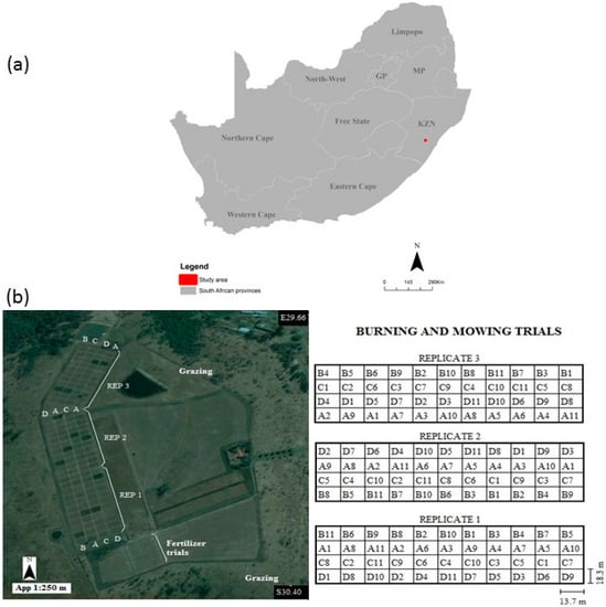
Figure 1.
(a) Location of the grassland sites at Ukulinga University of KwaZulu-Natal experimental Farm, Pietermaritzburg, South Africa; (b) shows the experimental setup and design at Ukulinga research farm (Image source: Google Earth).
2.2. Experimental Design
The experiment consisted of grass burning, mowing and fertilisation treatments at timely intervals. A total of 54 plots measuring 13.7 m × 18.3 m, with native grass growing under mowing and burning, were utilised in this study (Table 1). Burning treatments were undertaken at three levels, namely: (i) annually; (ii) biennially (after two years); and (iii) triennially (after three years). Mowing was also implemented at three levels. At Level 1, there was no mowing, at Level 2 grass was mown once in August, and at Level 3, grass was mown twice in August and after the first Spring rains.

Table 1.
Reflectance samples measured on each rangeland management treatment.
2.3. Field Campaign
To extract spectra from each plot, 20 points were randomly generated in a Geographic Information System (GIS) environment. Ultimately, 1080 points were derived from 54 plots and used to extract all WV-3 variables, using an overlay function in a GIS (Table 1). To test the capability of the combined red-edge and texture models in estimating above-ground grass biomass, we conducted a field survey on the 10 February 2016. During the field campaigns, plots with native grasses grown under mowing, burning, as well as no-treatment, were surveyed and the grass biomass clipped. The wet biomass of grass from each level of treatment was derived after cutting during the field survey. The samples were then taken to the laboratory, where moisture content was determined and dry grass biomass, hereafter referred to as above-ground grass biomass, was derived.
2.4. Remotely Sensed Data
A WorldView-3 image, acquired on a cloudless day on 16 February 2016, was used in this study to evaluate the strength of red-edge, combined with texture models, in predicting above-ground biomass. The WV-3 image has eight multispectral bands, i.e., coastal blue at 400–450 nm, blue at 450–510 nm, green at 510–589 nm, yellow at 585–625 nm, red at 630–690 nm, red-edge at 705–895 nm and two near-infrared bands, which overlap, at 770–895 and 860–1040 nm, respectively. The spatial resolution of all wavebands was 2 m. The image was first pre-processed to correct for the influence of atmospheric effects, using the Fast Line of Sight Atmospheric Analysis of Spectral Hypercubes (FLAASH), based on the parameters that were provided with the image. The FLAASH analysis was conducted after converting the image into radiance in Envi 5.2. Subsequently, the WorldView-3 image was geometrically corrected, based on ten locations measured using a handheld Trimble GeoXH 6000 global positioning system with a sub-meter accuracy. The image was then to resample using the first order polynomial transformation and nearest-neighbor resampling technique as in Sibanda et al. [37]. As mentioned earlier, the atmospherically corrected image was used in an overlay analysis, in conjunction with the point map, in order to derive spectral signatures of grass growing under different levels of grassland management treatments.
2.5. Modelling Above-Ground Grass Biomass
Single wavebands, broadband and red-edge vegetation indices, as well as grey level co-occurrence single-band and band-ratio texture models, were derived in Envi 4.3 from the pre-processed WV-3 image. The vegetation indices used in this study were chosen based on their optimal performance in literature [17,22]. Formulae for computing vegetation indices are detailed in Schumacher et al. [38]. The window sizes for deriving the grey-level co-occurrence texture models used in this study were 3 × 3, 5 × 5 and 7 × 7 pixels [39,40]. These window sizes were selected because their area was not bigger than that of a single plot of grass used in this study. The co-occurrence shifts considered in this study were 0:1, 1:1, 1:0, −1:1, 1:−1 which were chosen based on literature [30,41] and a quantization level of 64 was used in this study. The texture models computed in this study were mean, variance, homogeneity, contrast, dissimilarity, entropy, second moment and correlation. More details about the formulae for computing these texture models are summarised in Dube and Mutanga [30], as well as Schumacher et al. [38]. All the variables used in this study, and the formulae used to compute them, are detailed in Table 2. The derived spectral signatures were saved in a table format and exported to Microsoft Excel as comma separated values. These were then imported into Statistica Version 7 and R statistical software for statistical modelling.
Table 2.
Variable categories used in this study.
2.5.1. Statistical Modelling of Above-Ground Grass Biomass
The initial step was to conduct exploratory analysis and to derive descriptive statistics in Statistica Version 7. Under the exploratory data analysis procedure, we tested whether above-ground grass biomass data measured in the field significantly deviated (α = 0.05) from the normal distribution, based on the Lilliefors test. We then tested whether there was significant difference in the amount of above-ground biomass of grass grown under different levels of mowing and burning treatments based on analysis of variance and Tukey’s honest significant difference post hoc test.
2.5.2. Regression Modelling
In this study, we used Chun and Keleş’s [55] sparse partial least regression (SPLSR) algorithm. The SPLSR algorithm converts the variables into new orthogonal factors to circumvent multicollinearity and overfitting issues, considering the large number of variables used in this study. In converting the variables into orthogonal factors, SPLSR imparts sparsity into the models and then selects the optimal variables that correlate better to grass above-ground biomass. Because of these capabilities, SPLSR is appropriate for application on data with multicollinearity issues, such as the texture models of this study, relative to other algorithms (i.e., partial least squares regression (PLSR)) [55,56]. In this study, the aim was to test whether combining WV-3 optical texture models with red-edge derivatives improves accuracies. Therefore, SPLSR was chosen and utilised because of its ability to select optimal variables.
2.5.3. Assessing the Accuracy of Above-Ground Grass Biomass Models
To evaluate the accuracy of above-ground grass biomass models in this study, a leave-one-out cross-validation (LOOCV) procedure was followed, as detailed in Ritcher et al. [18]. In implementing the LOOCV procedure, 1080 samples, derived from 54 grassplots, were eliminated one by one and above-ground grass biomass estimation errors for each latent variable were derived. The latent variables that exhibited the least root mean square errors were considered as the optimal models for estimating above-ground grass biomass across different levels of grassland management treatments. We computed the coefficient of determination (R2), root mean square error (RMSEP) as well as the relative root mean square error (RMSEP_rel), as in Frazer et al. [57], to evaluate the models derived using band indices, as well as texture models. Models that exhibited small RMSEs and a high R2 were considered to be best in estimating above-ground biomass. Considering that SPLSR has the capability of identifying selecting optimal variables, we then used the variable importance (VIP) scores allocated for each of the selected variables by SPLSR, to distinguish the most influential ones from the best models [56].
Finally, an analysis of variance was used to test whether there were significant differences between the accuracies (RMSEP) of: (i) WV-3 wavebands; (ii) broadband Vis; (iii) Wavebands combined with broadband VIs; (iv) red-edge VIs; (v) combination of all VIs and wavebands; (vi) single-band texture models; (vii) combination of single-band and band-ratio texture models; and (viii) all variables combined in predicting above-ground biomass. These combinations were derived from literature [30,38]. Analysis of variance (ANOVA) was used after the normality test and it indicated that the data did not significantly deviate from the normal distribution.
2.5.4. Phases of Estimating Above-Ground Grass Biomass
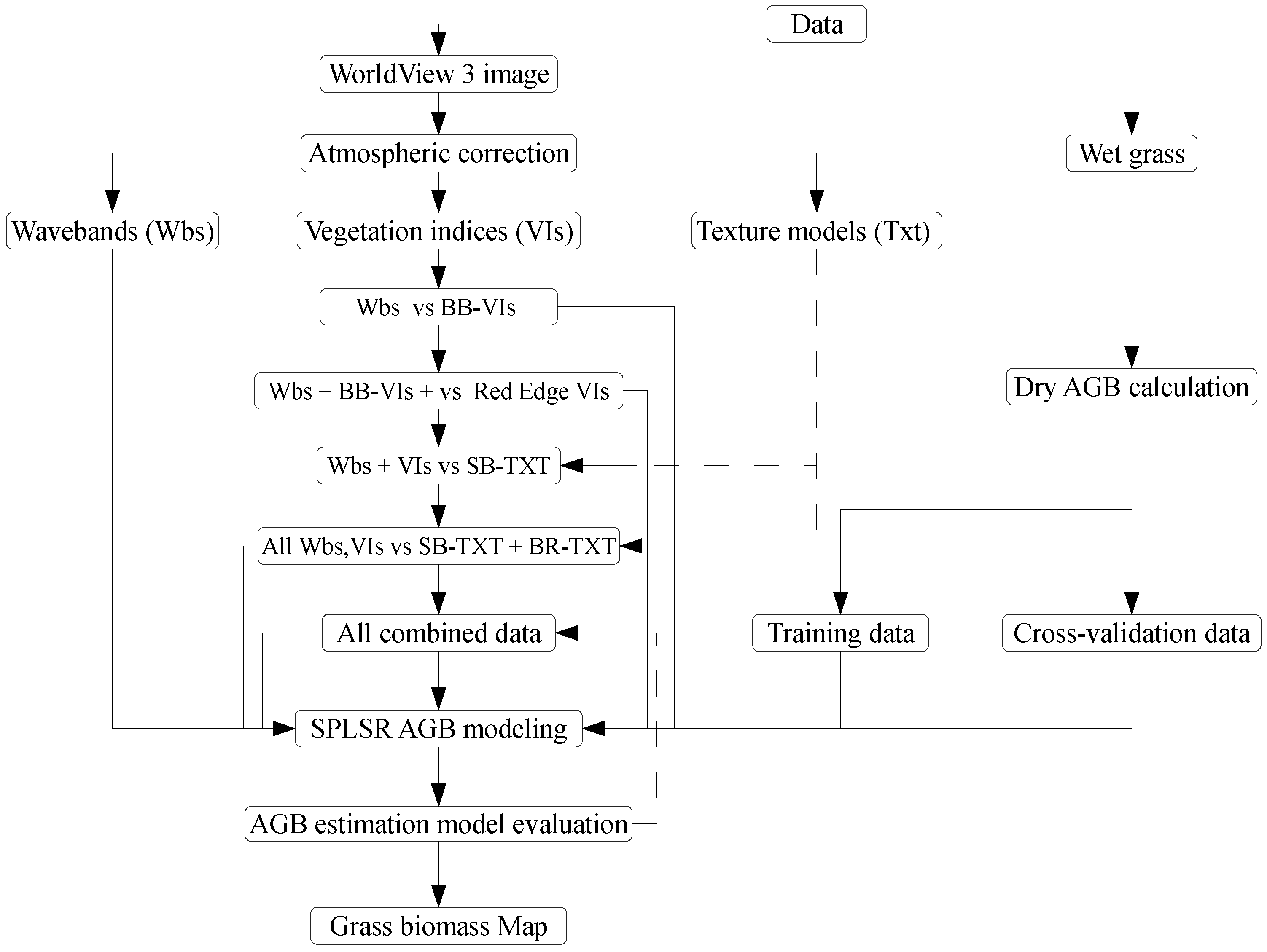
Table 2 summarises the four phases that were followed. In phase one, the strength of WV-3 wavebands was compared with that of broadband vegetation indices. In the second phase, wavebands were combined with broadband vegetation indices and then compared with the performance of red-edge vegetation indices. In the third phase, the wavebands, broadband and red-edge vegetation indices were combined and compared to the performance of single-band texture models. Lastly, the combination of all variables were then compared with the performance of all texture models. The optimal bands, indices and texture models that are derived using the variable selection capability of SPLSR were then used to estimate above-ground biomass across all grassland management treatments in this study. Figure 2 conceptually illustrates the phases followed.
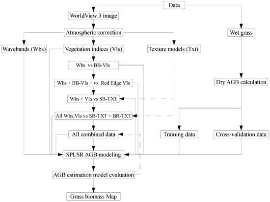
Figure 2.
Flowchart illustrating stages in estimating above-ground (ABG) grass biomass in this study. Wbs represents WV-3 wavebands, VIs are vegetation indices, BB-VIs are broadband vegetation indices, SB-TXT represents single band texture models and BR-TXT represents band ratio texture models.
3. Results
3.1. Descriptive Statistical Analysis and ANOVA Tests
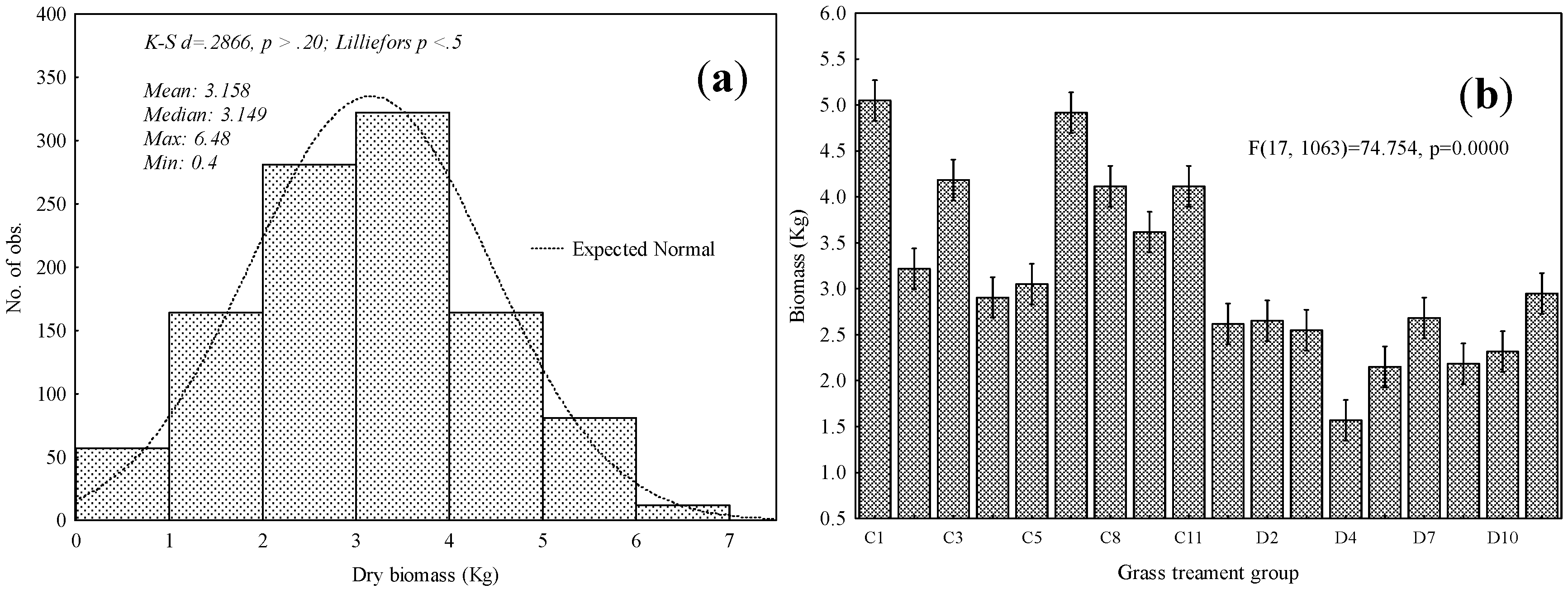
Normality test results based on the Lilliefors test, showed that above-ground grass biomass did not significantly deviate from the normal distribution (α = 0.05), as illustrated in Figure 3a. Consequently, ANOVA and SPLSR were then conducted. Figure 3a illustrates other descriptive statistics of grass above-ground biomass. The mean of 3.158 kg and a median of 3.149 kg were derived from the field-measured above-ground biomass of grass growing under different levels of burning and mowing treatments. Significant differences in the amount of above-ground biomass were observed amongst grasses growing under different grassland treatments (Figure 3b). Furthermore, Tukey’s HSD post hoc test showed that there were significant differences in the quantity of grass biomass between different pairs of burning and mowing grass treatments, as illustrated in Table 3 (p-value < 0.05).

Figure 3.
(a) Descriptive statistics of measured grass above-ground biomass; (b) significant difference amongst different levels of mowing and burning grassland management treatments based on analysis of variance test. Bars represent mean biomass of each management treatment level while whiskers represent confidence intervals of means at 95%.
Table 3.
Significant differences between different pairs of grass above-ground biomass grown under different levels of mowing and burning treatments, based on the Tukey’s HSD test.
3.2. Comparing the Performance of WorldView-3 Wavebands Combined with Broadband Vegetation Indices (Vis) and Red-Edge VIs in Estimating Above-Ground Grass Biomass
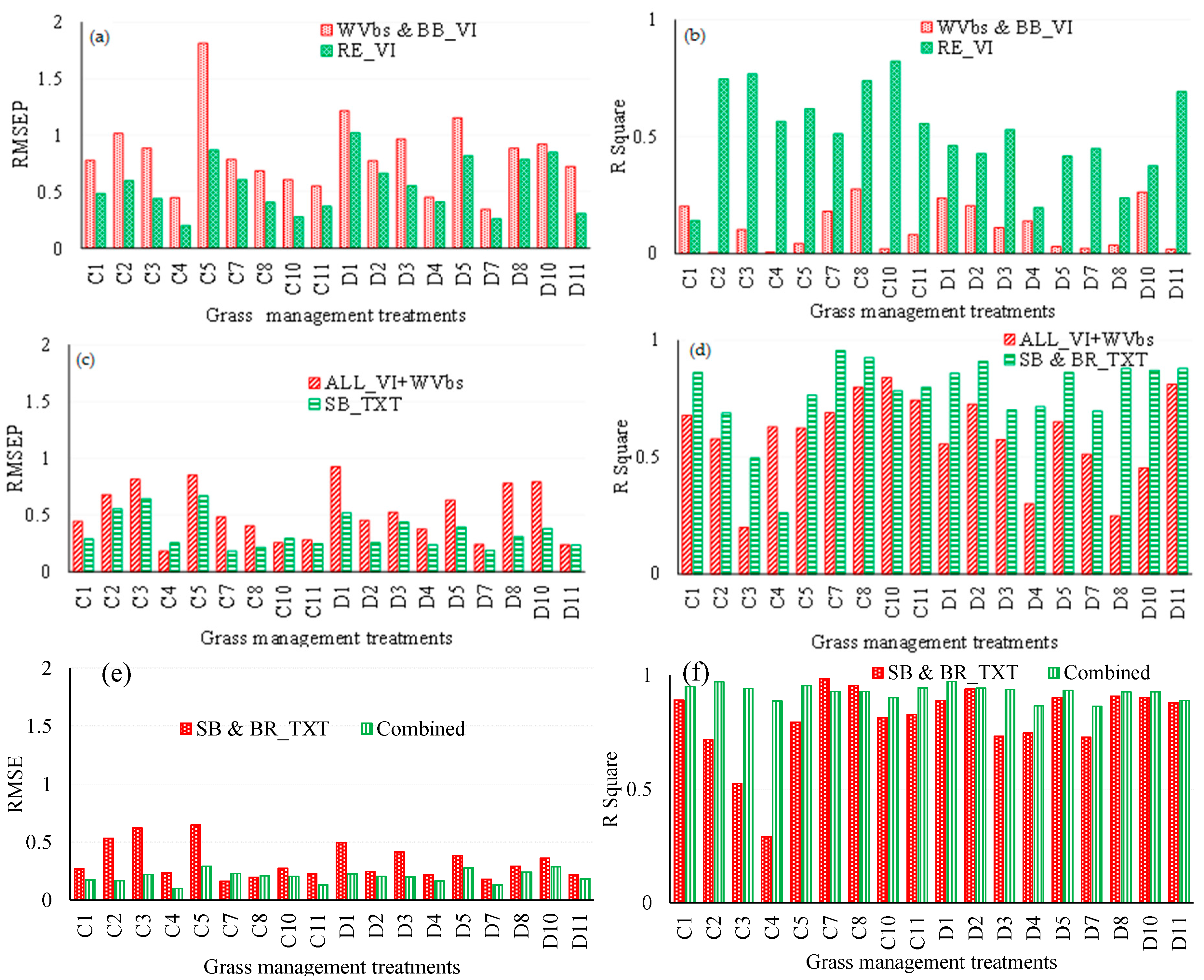
Exploring the possibility that WV-3 wavebands could better estimate above-ground biomass in relation to broadband VIs resulted in very small and very high RMSEP indicating poor model fitting. In that regard, those results were not presented. It can be observed from Figure 4a,b that the red-edge-derived vegetation indices performed better than broadband vegetation indices combined with band reflectance values. Red-edge-derived VIs resulted in higher accuracies (lower RMSEP), when compared with combined broadband VIs and band reflectance values. Specifically, triennial burning treatment D7 (R2 = 0.45, RMSEP = 0.26 kg/m2, RMSEPrel = 12.83) exhibited the lowest prediction error, when red-edge-derived vegetation indices were used. Meanwhile, the highest prediction errors obtained based on the red-edge vegetation indices were observed in C5 (R2 = 0.62, RMSEP = 0.87 kg/m2, RMSEPrel = 28.49). Red-edge-derived vegetation indices improved the accuracies of above-ground grass biomass estimation. However, relatively high prediction errors were observed from the triennial burn treatment D7 (R2 = 0.2, RMSEP = 0.34 kg/m2, RMSEPrel = 13) and C5 (R2 = 0.04, RMSEP = 1.81 kg/m2, RMSEPrel = 92.21), when WV-3 bands were combined with broadband vegetation indices in estimating above-ground grass biomass. The optimal red-edge indices that were selected were the normalized difference near-infrared red-edge index, the normalized difference red-edge index, the canopy chlorophyll content index, the tasseled cap: soil brightness index, and the anthocyanin reflectance index, in order of influence.
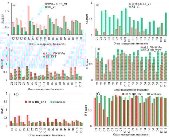
Figure 4.
A comparison of estimation accuracies derived using different WV-3 satellite data and its derivatives. Root mean square error of prediction (RMSEP) and R squares obtained in comparing (a,b) WV-3 combined BB_VIs and red-edge vegetation (RE_VIs) (c,d), all VIs combined with WVbs and single-band texture models (SB_TXT) and (e,f) SB_TXT) and all data combined. C1–11 and D1–11 are illustrated in Table 1.
3.3. Comparing the Performance of Single-Band Texture Models with All WV-3 VIs and Band Reflectance Values in Estimating Above-Ground Grass Biomass
The results of this study showed that the single-band texture models derived using the SPLSR algorithm predicted above-ground grass biomass better than all vegetation indices and wavebands combined. Figure 4c,d shows accuracies derived from using single-band texture models, as well as combined vegetation indices and wavebands. Based on single-band texture models, triennial burn treatments C7 (R2 = 0.51, RMSEP = 0.18 kg/m2, RMSEPrel = 5.56) had the least prediction errors. The single-band texture predictions had relatively lower estimation errors, when compared with all vegetation indices, combined with wavebands (C7 R2 = 0.18, RMSEP = 0.48 kg/m2, RMSEPrel = 9.83). When single-band texture models were used, the optimal window sizes were 3 × 3 and 5 × 5 at [0:1] and [1:1] offsets. The mean, dissimilarity, homogeneity entropy, correlation, variance and second moment texture model types were frequently selected as optimal variables at this stage, based on the SPLSR algorithm. In this study, the single-band texture and band-ratio texture models did not perform significantly differently, hence those results were not included in this study.
3.4. Comparing the Performance of Combined Single-Band and Band-Ratio Texture Models with the Combination of All WV-3 VIs, Band Reflectance Values and Single-Band Texture Models in Estimating Above-Ground Grass Biomass
Results of this work also showed that all data combined (texture indices, vegetation indices a nd spectral wavebands), outperformed the texture models (i.e., single-band and band-ratio texture). Texture models individually exhibited slightly higher prediction errors when compared to the combination of single-band texture models’ vegetation indices and wavebands. Based on all variables combined, biennial burn treatments C4 (R2 = 0.89, RMSEP = 0.1 kg/m2, RMSEPrel = 3.45) had the lowest estimation errors. The combination of texture models resulted in comparatively lower accuracies with higher errors (C4: R2 = 0.29, RMSEP = 0.22 kg/m2, RMSEPrel = 5.61) (see Figure 4e,f).
3.5. Estimating Above-Ground Grass Biomass across Different Levels of Grassland Management Treatments Using WV-3-Derived Texture Models Combined with Optimal Vegetation Indices Selected by the SPLSR Algorithm
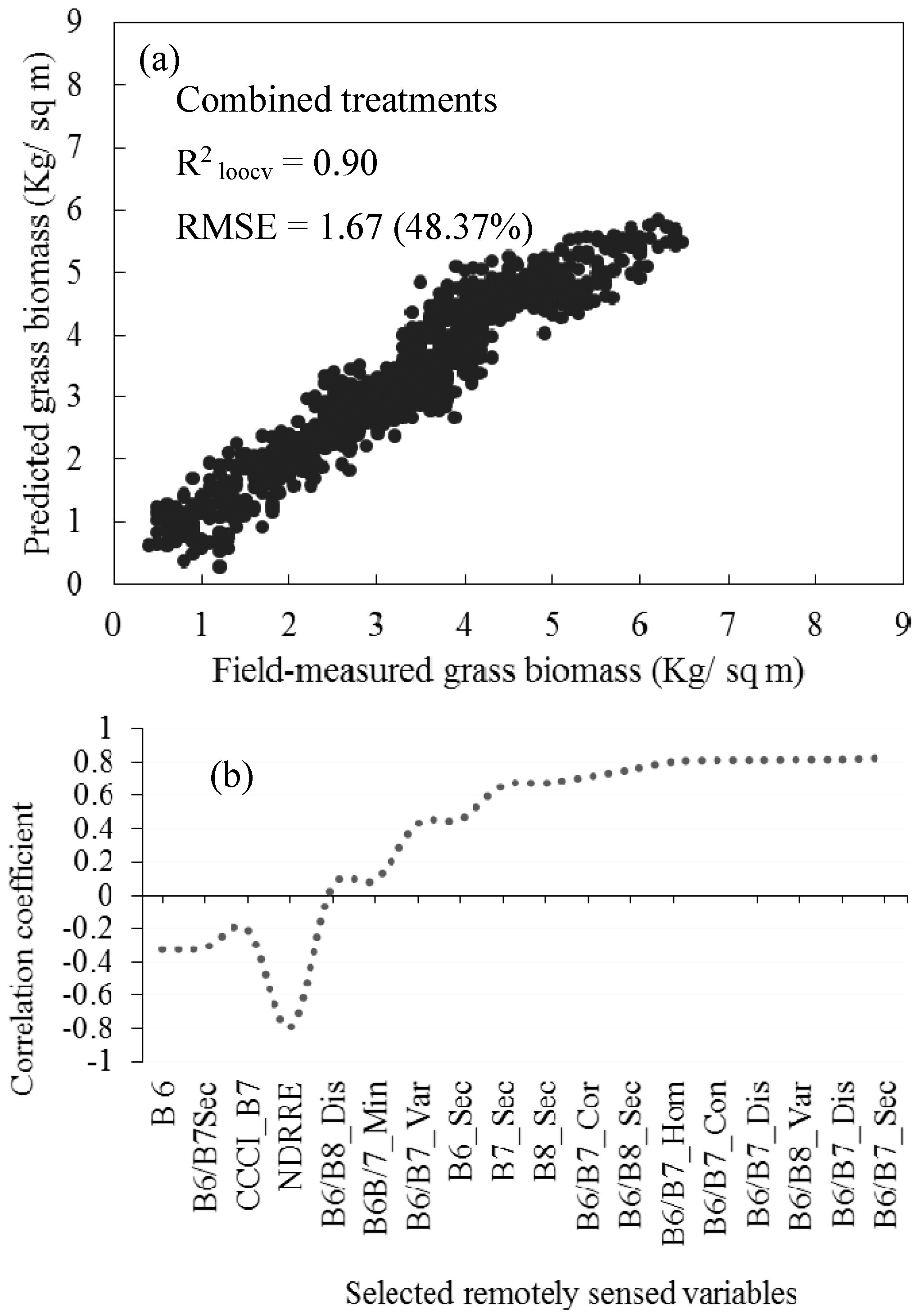
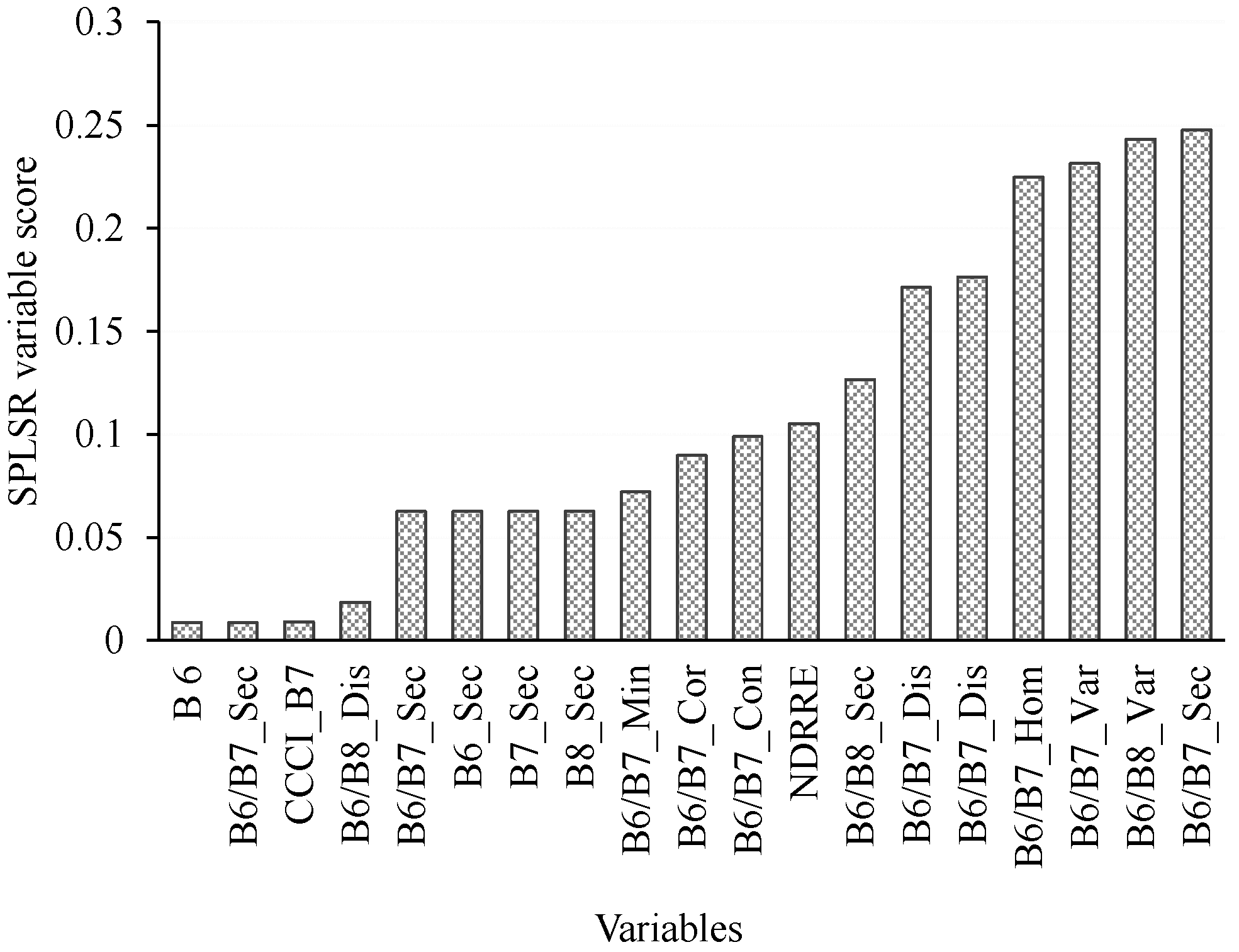
When all data were combined and all treatments pooled, a comparatively lower prediction error was obtained, as illustrated in Figure 5. Further analysis (Figure 5b) illustrated that the stray points on Figure 5a were induced by those variables which exhibited low correlation coefficients such as B6, B6/B7 and NDRRE. However, the overall influence of stray points on error was minimal as indicated by an observed R2 of 0.90 and RMSEP of 1.67 kg/m2. It was also observed that the red-edge-derived texture and vegetation indices were the most influential variables that produced relatively lower accuracies (Figure 6). From the selected variables, the 5 × 5 second moment and variance simple band-ratio texture models derived from Bands 6 and 7 exhibited the highest scores in this study.
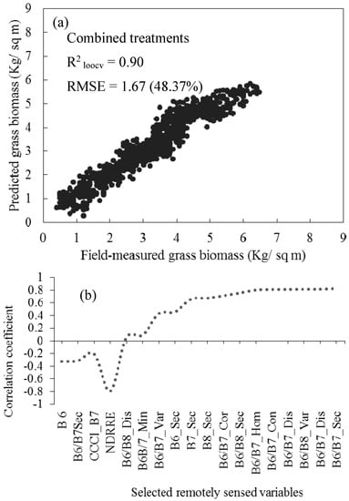
Figure 5.
(a) Relationship between the field-measured and estimated grass above-ground biomass across all grass management treatments for validating sparse partial least regression (SPLSR) models, based on the leave-one-out cross-validation procedure. Note that the relative root mean square error is presented as a percentage; (b) illustrates the relationship between all the optimal variables and grass biomass across all treatments.

Figure 6.
Best variables selected using SPLSR, in estimating above-ground grass biomass across different grassland management treatments. Note that on ‘B6/B7’ represents the ratio of WV-3 Bands 6 and 7 and NDRE is the normalized difference red-edge index.
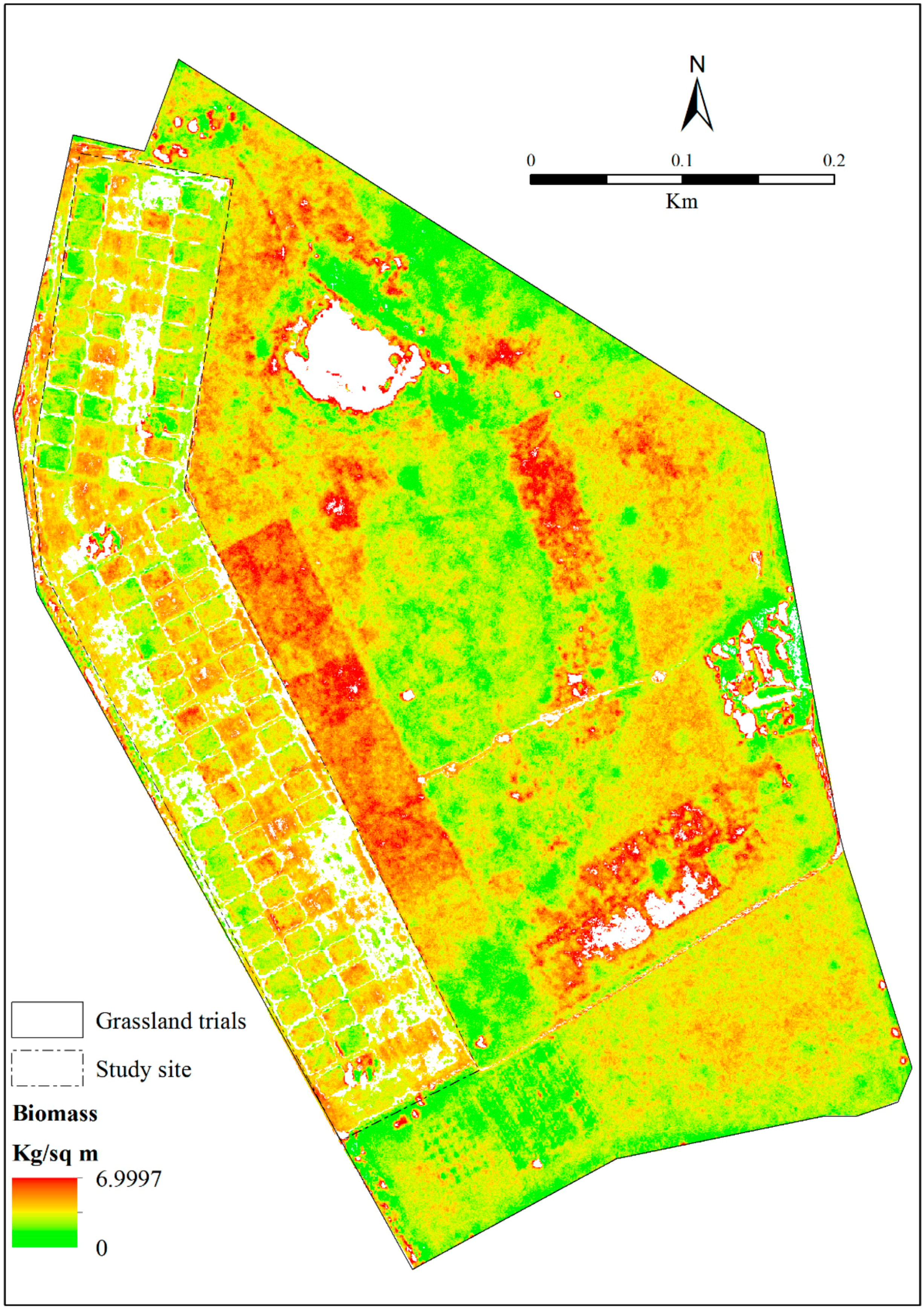
Figure 7 illustrates the spatial distribution of above-ground biomass (ABGB) across different levels of mowing and burning treatments. It can be observed that the triennial (C8) and biennial C5) treatments accumulate more biomass, compared to the annual burn (D3). On the other hand, the mowing treatments (C10) show less ABGB accumulation, due to the high removal of grass.
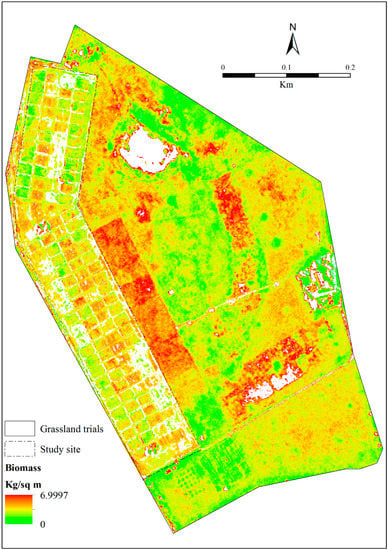
Figure 7.
Spatial distribution of biomass across different grassland management treatments.
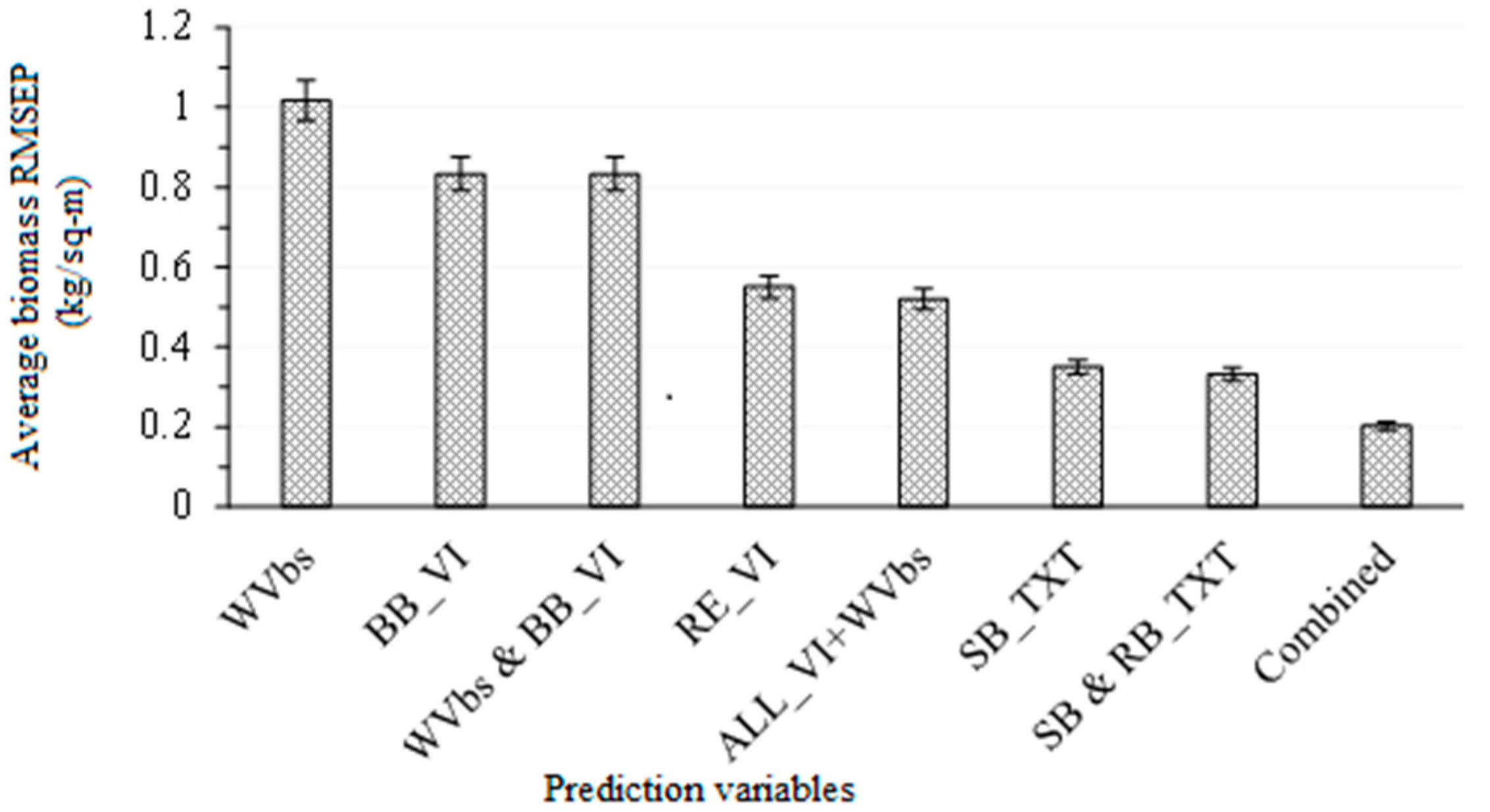
Figure 8 summarises the accuracies obtained, using single wavebands, broadband vegetation indices, red-edge vegetation indices, single-band and band-ratio texture models, in predicting ABGB across different levels of mowing and burning treatments. When single wavebands were used in estimating above-ground grass biomass, an average RMSEP of 1.02 kg/m2 was obtained. These variables had the highest RMSEP and were the least accurate predictors for estimating grass ABGB in this study. The accuracy of estimating ABGB slightly improved to an average RMSEP of 0.83, 1.02 kg/m2, when broadband vegetation indices were used. However, combining the broadband vegetation indices did not significantly improve the accuracy of ABGB estimation, as illustrated in Figure 8. The red-edge vegetation indices significantly improved the accuracy of ABGB estimation to average RMSEP: 0.55 kg/m2. The combination of red-edge vegetation indices with broadband vegetation indices, as well as single wavebands, did not significantly improve the accuracy of estimating grass ABGB in this study. When single-band grey level co-occurrence texture matrices were used the ABGB prediction accuracy significantly improved (average RMSEP: 0.35 kg/m2). In comparison, the combination of single-band and band-ratio texture models did not significantly improve the accuracy of estimating ABGB. When all variables were combined (red-edge and texture models), optimal accuracies (average RMSEP: 0.2 kg/m2) were obtained in this study.
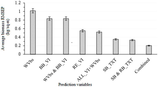
Figure 8.
Average RMSEPs derived in predicting above-ground biomass, using WV-3 wavebands (WVbs) broadband (BB_VI), red-edge (RE_VI), single-band (SB_TXT), band-ratio texture (BR_TXT) indices and all combined data across different rangeland management treatments. Whiskers represent the upper and lower confidence intervals of the mean.
4. Discussion
This study tested the robustness of combining texture models with red-edge in estimating the ABGB across different rangeland management treatments, based on the recently launched WorldView-3 EO data. This study specifically sought to find out whether the integration of the red-edge with grey level co-occurrence texture models, extracted at different window sizes and offsets, could improve the accuracy of models for predicting grass above-ground biomass across different levels of mowing and burning treatments in the context of southern African grasslands.
4.1. Combining Texture Models with Red-Edge in Predicting above-Ground Grass Biomass
The findings of this study suggest that combining texture metrics and red-edge-derived vegetation indices has relatively higher prospects of improving the estimation accuracy of ABGB growing across different levels of grassland management treatments, when compared to the performance of texture metrics as stand-alone data.
This could be attributed to the sensitivity of the red-edge section of the electromagnetic spectrum to the variations in LAI and LAD changes [58,59], as well as foliar chlorophyll variability caused by different levels of mowing, and the influx of post-fire nutrients [60]. During the mowing process, grass twigs and leaves are reduced, according to different mowing treatment levels. This results in the alteration of the grass LAI as well as LAD across different levels of mowing. Accordingly, the spectral reflectance from these mowing different levels is better detected by the red-edge section of the electromagnetic spectrum, augmenting the performance of texture models. Furthermore, the red-edge is also sensitive to the variability in chlorophyll content, which accumulates after the burning treatment of grass. This also facilitates an improvement in the accuracy of the estimation of grass biomass, when the red-edge is combined with texture models.
Meanwhile, the textural variables are sensitive to the geographical distribution of minute, but crucial, tonal grass variations in the image induced by the reflectance of different levels of grassland management treatments on certain spectral bands, such as the red-edge and its derived band ratios [61]. This boosts the robustness of texture models and red-edge variables in estimating ABGB. Furthermore, texture is also sensitive to the variations in LAI and LAD induced by mowing, as well as the high chlorophyll content from post-fire nutrients in those grasses grown under different levels of burning and mowing treatments. Subsequently, high estimation accuracies of above-ground grass biomass are realised when texture models are combined with the red-edge derivatives. In addition texture optimises the characterisation of spatial information independently of the tone, while increasing the range of biomass to optimal levels [8]. This facilitates robustness and a plausible performance, when texture metrics are combined with red-edge waveband derivatives, optimising the accurate estimation of ABGB across complex grassland management treatments in this study. Our results are consistent with those of Zhang et al. [62], who noted that the models derived from a combination of spectrum and texture models of the Chinese high-resolution remote sensing satellite Gaofen-1, increased the estimation accuracies of Populus euphratica forest when compared with the performance of reflectance or texture models. In another similar study, Takayama and Iwasaki [63] showed that the combination of the spatial and spectral information from spectral responses and texture models optimally improved the estimation accuracies of tropical vegetation biomass from a RMSE of 66.16 t/ha to a RMSE of 62.62 t/ha in Hampangen, Central Kalimantan, Indonesia, based on WV-3 satellite data. Kelsey and Neff [53] also demonstrated that texture models improved the estimation of vegetation biomass at the San Juan National Forest in southwest Colorado, USA, from a RMSE of 56.4 to a RMSE of 45.6, based on Landsat data.
Results of this study also indicated that the single-band texture metrics improved the accuracy of ABGB estimation relative to red-edge and broadband VI, combined with single wave bands. This is because texture metrics are renowned for accurately capturing the heterogeneity of vegetation structural traits when compared to vegetation indices as a stand-alone dataset [29,32]. The local variance within pixels at a defined neighbourhood, induced by different levels of mowing and burning treatments in this study, is better distinguished by the texture variables when compared with their spectral signature variations at various WorldView-3 wavelengths. Specifically, the spectral responses of vegetation are computed on a pixel basis, while texture is computed from a desired neighbourhood of pixels that is adjustable, increasing the prospects of texture in credibly predicting biomass better than broadband and spectral reflectance [53].
Furthermore, the optimal performance of texture variables, in relation to red-edge and other wavebands and indices in this study, could be explained by the fact that the saturation levels of texture metrics in estimating biomass are considerably higher when compared to those of vegetation indices, such as NDVI, which saturate at lower levels of biomass [64,65]. This results in the underestimation of ABGB. In addition, the distinctive performance of texture models could also be attributed to the fact that the band-ratio textures are an amalgamation of strengths derived from different spectral wavebands, combined with image tone variations. This increases the sensitivity of texture and red-edge models to the spatial characteristics of different grass canopies, hence facilitating a comparatively higher estimation accuracy of ABGB, a mammoth challenge when using vegetation indices.
Our results are consistent with those of a growing body of literature that attests the optimal performance of grey level texture models, when compared to all vegetation indices [32,64,66]. For example, Zhang et al. [62] noted that when texture models from a high spatial resolution (2 and 16 m) GoaFen-1 optical EO data were integrated, the accuracy of above-ground of the Populus euphratica forest. In a related study, Sarker and Nichol [7] concluded that the spectral reflectance and traditional vegetation indices have low prospects for estimating biomass, when compared with texture models. Specifically, Sarker and Nichol [7] noted that texture models derived from ALSO AVNIR-2 improved the vegetation biomass estimation from a RMSE of 64 t/ha, based on traditional vegetation indices and spectral reflectance to a RMSE of 46 t/ha, as noted in this study. However, Sarker and Nichol’s [46] results showed that band ratios further improved the accuracy of estimating biomass to a RMSE of 32 t/ha. Their results are contrary to those of this study, which indicated that band-ratio and single-band texture models did not perform significantly differently when predicting ABGB across different levels of grassland management treatments.
Furthermore, results of this study showed that the red-edge waveband derivatives improved the accuracy of the models for predicting ABGB at different grassland management treatments, when compared to broadband vegetation indices combined with wavebands. Based on the results of this study, the red-edge bands outperformed the broadband vegetation indices, combined with raw wavebands. These results were somewhat expected, as this has been noted in literature. This can be explained by the fact that the red-edge portion of the electromagnetic spectrum is highly sensitive to changes in the grass chlorophyll [67], induced by disturbances such as mowing and burning. Post-fire foliar nutrients, which are rich in nitrogen and phosphorus, induce high chlorophyll concentrations in the grass, which is then detected by the red-edge waveband derivatives in this study.
Meanwhile, the decreases in the leaf area distribution and LAI, due to mowing activities, induces a variation in the signature of grass, which is then detected better by the red-edge derivatives, when compared with the single wavebands and broadband vegetation indices. Our results are consistent with those found in a growing body of contemporary literature [68,69,70,71]. For instance, Fernández-Manso et al. [44] noted that red-edge derivatives detected the fire activities better and with higher accuracies (Modified Simple Ratio red-edge narrow R2: 0.69), when compared to single wave bands and broadband vegetation indices (Red band R2: 0.093, NIR R2: 0.63, and NDVI R2: 0.43) in Sierra de Gata (central-western Spain), based on Sentinel data. Gara, et al. [70] also noted that the inclusion of red-edge derivatives also improved the estimation of carbon stocks from an explained variance of 63%, based on NDVI, to 70% in the savanna dry forest of Zimbabwe.
4.2. Biological Behavior of Grasses at Ukulinga Research Farm Based on Literature Review
As highlighted earlier, mowing through defoliation reduces grass LAI as well as LAD. This markedly reduces the relative abundance of the dominant Themeda triandra (which is a highly palatable grass species), overall grass basal cover as well as the biomass [72]. The changes in grass species composition and dominance then could explain the spatial variability of grass biomass noted in this study. Furthermore, mowing at Ukulinga increased sward productivity in the season following the removal treatment when compared to burning which promotes growth of grasses with higher protein content [72]. This is illustrated by high estimates of biomass in some mowing (C10 and 11 as well as D10 and 11) treatments in relation to other burning treatments (C2 and 3 as well D2 and 3) in the results of this study through high biomass. Treatments with frequent fire administration would yield a variety of short grasses dominated by a Themeda triandra, Hyparrhenia hirta and Tristachya leucothrix as shown by Kirkman et al. [73] which could also explain some of the variabilities observed in treatments such as C1 and 2 with annual burning relative to other treatments. Kirkman et al. [73] reported that there is a high replacement rate of the dominant grass species between annually burned and unburned treatments at Ukulinga. These findings by Kirkman et al. [73] are in agreement with the results of this study which indicate a variability in the estimated ABGB between annually burned and the control treatments. Furthermore research shows that biennially burnt treatments tend to produce more biomass, on average, than treatments burnt less frequently or mown annually in winter [74]. Above all, the effects of mowing and burning, as well as their interaction on native grasses still requires further studies [75] especially from a remote sensing context.
5. Conclusions
The aim of this study was to assess the accuracy of combining red-edge derivatives with texture models in predicting the above-ground biomass of grass growing under different levels of grassland management treatments. Based on the findings of this study, we conclude that:
- combining texture models with red-edge derivatives provides a more accurate approach in estimating the above-ground biomass of grass grown under complex grassland management treatments. To the best of our knowledge, this is the first study to evaluate the utility of texture models and red-edge in estimating above-ground grass biomass, across a multitude of grassland management treatment levels,
- the best predictor in estimating above-ground biomass (ABGB) grown under complex grassland management treatments was derived using all data combined,
- texture models perform better than the red-edge vegetation indices in estimating grass above-ground biomass, and
- as expected, the red-edge spectrum-derived vegetation indices outperformed the broadband indices.
In testing specific objectives, our results suggests that (i) broadband vegetation indices such as normalised difference vegetation index (NDVI), enhanced vegetation index (EVI) and soil-adjusted vegetation index (SAVI) are comparatively better predictors of ABGB WorldView-3 (WV-3) standard wavebands; (ii) red-edge-derived vegetation indices are better predictors than standard wave bands combined with broadband vegetation indices; (iii) texture models are better predictors of ABGB in relation to red-edge, broadband vegetation indices (Vis) combined with all WV-3 bands; (iv) band texture ratios are better predictors of ABGB across different treatments when compared to all variables combined. Ultimately, when all variables were combined, red-edge VI texture and band-ratio texture exhibited optimal ABGB predictions in this study. The results of this work give insights into the estimation of grass biomass in complex grassland management treatments of arid tropical region grasses. The bulk of the studies that have demonstrated the utility of texture variables in above-ground biomass estimation have focused on the forests and crops of America and Europe. Therefore, to the best of our knowledge, the results of this study demonstrate, for the first time, the utility of texture models combined with red-edge waveband derivatives in estimating above-ground grass biomass across the complex grassland management treatments of the arid tropics, characterised by a high soil background effect. These results are an important footstool upon which critical spatial information required for grassland policy-making and sustainable grassland management in southern Africa could be derived.
Acknowledgments
The authors are grateful to the University of KwaZulu-Natal/National Research Fund and KwaZulu-Natal Sandstone Sourveld (KZNSS) forum, in conjunction with the eThekwini Municipality, also known as the DRAP, for funding this research. The authors would also like to thank K. Kirkman, Alison Young, Deepa Mangesh, T. Dube, Terence D Mushore, Thulile Vundla and Reneilwe Maake, for their assistance with field work, data collection and analysis as well as proofreading the manuscript. Finally, the authors extend their gratitude to the reviewers for their constructive criticism.
Author Contributions
Mbulisi Sibanda conceived and performed the experiment, collected data, analysed the data and wrote the paper under the supervision of Onisimo Mutanga, Mathieu Rouget and Lalit Kumar. Onisimo Mutanga, Mathieu Rouget and Lalit Kumar also edited the manuscript. Furthermore, Mathieu Rouget provided the funds for conducting this research. The research funds were provided by eThekwini Municipality through the Durban Research Action Partnership: KwaZulu-Natal Sandstone Sourveld Programme and the South African Research Chairs Initiative of the Department of Science and Technology and the National Research Foundation of South Africa (grant No. 84157).
Conflicts of Interest
The authors declare no conflict of interest.
References
- Kumar, L.; Sinha, P.; Taylor, S.; Alqurashi, A.F. Review of the use of remote sensing for biomass estimation to support renewable energy generation. J. Appl. Remote Sens. 2015, 9, 097696. [Google Scholar] [CrossRef]
- Wilson, J.B.; Peet, R.K.; Dengler, J.; Pärtel, M. Plant species richness: The world records. J. Veg. Sci. 2012, 23, 796–802. [Google Scholar] [CrossRef]
- O’Mara, F.P. The role of grasslands in food security and climate change. Ann. Bot. 2012, 110, 1263–1270. [Google Scholar] [CrossRef] [PubMed]
- Andrade, B.O.; Koch, C.; Boldrini, I.I.; Vélez-Martin, E.; Hasenack, H.; Hermann, J.-M.; Kollmann, J.; Pillar, V.D.; Overbeck, G.E. Grassland degradation and restoration: A conceptual framework of stages and thresholds illustrated by southern Brazilian grasslands. Nat. Conserv. 2015, 13, 95–104. [Google Scholar] [CrossRef]
- Conant, R.T.; Paustian, K.; Elliott, E.T. Grassland management and conversion into grassland: Effects on soil carbon. Ecol. Appl. 2001, 11, 343–355. [Google Scholar] [CrossRef]
- Bastin, J.-F.; Barbier, N.; Couteron, P.; Adams, B.; Shapiro, A.; Bogaert, J.; De Cannière, C. Aboveground biomass mapping of African forest mosaics using canopy texture analysis: Toward a regional approach. Ecol. Appl. 2014, 24, 1984–2001. [Google Scholar] [CrossRef]
- Sarker, L.R.; Nichol, J.E. Improved forest biomass estimates using ALOS AVNIR-2 texture indices. Remote Sens. Environ. 2011, 115, 968–977. [Google Scholar] [CrossRef]
- Rosenqvist, Å.; Milne, A.; Lucas, R.; Imhoff, M.; Dobson, C. A review of remote sensing technology in support of the Kyoto Protocol. Environ. Sci. Policy 2003, 6, 441–455. [Google Scholar] [CrossRef]
- Lu, D. The potential and challenge of remote sensing-based biomass estimation. Int. J. Remote Sens. 2006, 27, 1297–1328. [Google Scholar] [CrossRef]
- Meng, S.; Pang, Y.; Zhang, Z.; Jia, W.; Li, Z. Mapping Aboveground Biomass using Texture Indices from Aerial Photos in a Temperate Forest of Northeastern China. Remote Sens. 2016, 8, 230. [Google Scholar] [CrossRef]
- Timothy, D.; Onisimo, M.; Riyad, I. Quantifying aboveground biomass in African environments: A review of the trade-offs between sensor estimation accuracy and costs. Trop. Ecol. 2016, 57, 393–405. [Google Scholar]
- Schino, G.; Borfecchia, F.; De Cecco, L.; Dibari, C.; Iannetta, M.; Martini, S.; Pedrotti, F. Satellite estimate of grass biomass in a mountainous range in central Italy. Agrofor. Syst. 2003, 59, 157–162. [Google Scholar] [CrossRef]
- Griffith, J.A.; Price, K.P.; Martinko, E.A. A multivariate analysis of biophysical parameters of tallgrass prairie among land management practices and years. Environ. Monit. Assess. 2001, 68, 249–271. [Google Scholar] [CrossRef] [PubMed]
- Xie, Y.; Sha, Z.; Yu, M.; Bai, Y.; Zhang, L. A comparison of two models with Landsat data for estimating above ground grassland biomass in Inner Mongolia, China. Ecol. Model. 2009, 220, 1810–1818. [Google Scholar] [CrossRef]
- Huete, A.R. Separation of soil-plant spectral mixtures by factor analysis. Remote Sens. Environ. 1986, 19, 237–251. [Google Scholar] [CrossRef]
- Bannari, A.; Morin, D.; Bonn, F.; Huete, A. A review of vegetation indices. Remote Sens. Rev. 1995, 13, 95–120. [Google Scholar] [CrossRef]
- Mutanga, O.; Skidmore, A.K. Narrow band vegetation indices overcome the saturation problem in biomass estimation. Int. J. Remote Sens. 2004, 25, 3999–4014. [Google Scholar] [CrossRef]
- Nichol, J.E.; Sarker, M.L.R. Improved biomass estimation using the texture parameters of two high-resolution optical sensors. IEEE Trans. Geosci. Remote Sens. 2011, 49, 930–948. [Google Scholar] [CrossRef]
- Ngubane, Z.; Odindi, J.; Mutanga, O.; Slotow, R. Assessment of the Contribution of WorldView-2 Strategically Positioned Bands in Bracken fern (Pteridium aquilinum (L.) Kuhn) Mapping. S. Afr. J. Geomat. 2014, 3, 210–223. [Google Scholar] [CrossRef]
- Ramoelo, A.; Skidmore, A.K.; Cho, M.A.; Schlerf, M.; Mathieu, R.; Heitkönig, I.M. Regional estimation of savanna grass nitrogen using the red-edge band of the spaceborne RapidEye sensor. Int. J. Appl. Earth Obs. Geoinf. 2012, 19, 151–162. [Google Scholar] [CrossRef]
- Zhao, P.; Lu, D.; Wang, G.; Wu, C.; Huang, Y.; Yu, S. Examining Spectral Reflectance Saturation in Landsat Imagery and Corresponding Solutions to Improve Forest Aboveground Biomass Estimation. Remote Sens. 2016, 8, 469. [Google Scholar] [CrossRef]
- Broge, N.H.; Leblanc, E. Comparing prediction power and stability of broadband and hyperspectral vegetation indices for estimation of green leaf area index and canopy chlorophyll density. Remote Sens. Environ. 2001, 76, 156–172. [Google Scholar] [CrossRef]
- Pu, R.; Gong, P.; Biging, G.S.; Larrieu, M.R. Extraction of red edge optical parameters from Hyperion data for estimation of forest leaf area index. IEEE Trans. Geosci. Remote Sens. 2003, 41, 916–921. [Google Scholar]
- Delegido, J.; Verrelst, J.; Rivera, J.P.; Ruiz-Verdú, A.; Moreno, J. Brown and green LAI mapping through spectral indices. Int. J. Appl. Earth Obs. Geoinf. 2015, 35, 350–358. [Google Scholar] [CrossRef]
- Curran, P.J.; Dungan, J.L.; Gholz, H.L. Exploring the relationship between reflectance red edge and chlorophyll content in slash pine. Tree Physiol. 1990, 7, 33–48. [Google Scholar] [CrossRef] [PubMed]
- Asner, G.P. Biophysical and biochemical sources of variability in canopy reflectance. Remote Sens. Environ. 1998, 64, 234–253. [Google Scholar] [CrossRef]
- Lu, D. Aboveground biomass estimation using Landsat TM data in the Brazilian Amazon. Int. J. Remote Sens. 2005, 26, 2509–2525. [Google Scholar] [CrossRef]
- Cutler, M.; Boyd, D.; Foody, G.; Vetrivel, A. Estimating tropical forest biomass with a combination of SAR image texture and Landsat TM data: An assessment of predictions between regions. ISPRS J. Photogramm. Remote Sens. 2012, 70, 66–77. [Google Scholar] [CrossRef]
- Eckert, S. Improved forest biomass and carbon estimations using texture measures from WorldView-2 satellite data. Remote Sens. 2012, 4, 810–829. [Google Scholar] [CrossRef]
- Dube, T.; Mutanga, O. Investigating the robustness of the new Landsat-8 Operational Land Imager derived texture metrics in estimating plantation forest aboveground biomass in resource constrained areas. ISPRS J. Photogramm. Remote Sens. 2015, 108, 12–32. [Google Scholar] [CrossRef]
- Wallis, C.I.; Paulsch, D.; Zeilinger, J.; Silva, B.; Fernández, G.F.C.; Brandl, R.; Farwig, N.; Bendix, J. Contrasting performance of Lidar and optical texture models in predicting avian diversity in a tropical mountain forest. Remote Sens. Environ. 2016, 174, 223–232. [Google Scholar] [CrossRef]
- Ozdemir, I.; Karnieli, A. Predicting forest structural parameters using the image texture derived from WorldView-2 multispectral imagery in a dryland forest, Israel. Int. J. Appl. Earth Obs. Geoinf. 2011, 13, 701–710. [Google Scholar] [CrossRef]
- Salas, E.A.L.; Boykin, K.G.; Valdez, R. Multispectral and Texture Feature Application in Image-Object Analysis of Summer Vegetation in Eastern Tajikistan Pamirs. Remote Sens. 2016, 8, 78. [Google Scholar] [CrossRef]
- Fynn, R.W.; O’Connor, T.G. Determinants of community organization of a South African mesic grassland. J. Veg. Sci. 2005, 16, 93–102. [Google Scholar] [CrossRef]
- Morris, C.; Fynn, R. The Ukulinga long-term grassland trials: Reaping the fruits of meticulous, patient research. Bull. Grassl. Soc. South. Afr. 2001, 11, 7–22. [Google Scholar]
- De Wit, M.; Blignaut, J.; Nazare, F. Monetary Valuation of the Grasslands in South Africa. 2006. Available online: http://biodiversityadvisor.sanbi.org/wp-content/uploads/2014/07/2006deWit_Background-InfoRep5_Strategic-Monetary-valuation.pdf (accessed on 6 January 2017).
- Sibanda, M.; Mutanga, O.; Rouget, M. Testing the capabilities of the new WorldView-3 spaceborne sensor’s red-edge spectral band in discriminating and mapping complex grassland management treatments. Int. J. Remote Sens. 2017, 38, 1–22. [Google Scholar] [CrossRef]
- Schumacher, P.; Mislimshoeva, B.; Brenning, A.; Zandler, H.; Brandt, M.; Samimi, C.; Koellner, T. Do Red Edge and Texture Attributes from High-Resolution Satellite Data Improve Wood Volume Estimation in a Semi-Arid Mountainous Region? Remote Sens. 2016, 8, 540. [Google Scholar] [CrossRef]
- Chica-Olmo, M.; Abarca-Hernandez, F. Computing geostatistical image texture for remotely sensed data classification. Comput. Geosci. 2000, 26, 373–383. [Google Scholar] [CrossRef]
- Wang, L.; Sousa, W.P.; Gong, P.; Biging, G.S. Comparison of IKONOS and QuickBird images for mapping mangrove species on the Caribbean coast of Panama. Remote Sens. Environ. 2004, 91, 432–440. [Google Scholar] [CrossRef]
- Safari, A.; Sohrabi, H. Ability of Landsat-8 OLI derived texture metrics in estimating aboveground carbon stocks of coppice Oak Forests. ISPRS Int. Arch. Photogramm. Remote Sens. Spat. Inf. Sci. 2016, 751–754. [Google Scholar] [CrossRef]
- Kang, Y.; Özdoğan, M.; Zipper, S.C.; Román, M.O.; Walker, J.; Hong, S.Y.; Marshall, M.; Magliulo, V.; Moreno, J.; Alonso, L. How Universal Is the Relationship between Remotely Sensed Vegetation Indices and Crop Leaf Area Index? A Global Assessment. Remote Sens. 2016, 8, 597. [Google Scholar] [CrossRef]
- Gitelson, A.A.; Merzlyak, M.N. Remote estimation of chlorophyll content in higher plant leaves. Int. J. Remote Sens. 1997, 18, 2691–2697. [Google Scholar] [CrossRef]
- Fernández-Manso, A.; Fernández-Manso, O.; Quintano, C. SENTINEL-2A red-edge spectral indices suitability for discriminating burn severity. Int. J. Appl. Earth Obs. Geoinf. 2016, 50, 170–175. [Google Scholar] [CrossRef]
- Santoso, H.; Gunawan, T.; Jatmiko, R.H.; Darmosarkoro, W.; Minasny, B. Mapping and identifying basal stem rot disease in oil palms in North Sumatra with QuickBird imagery. Precis. Agric. 2011, 12, 233–248. [Google Scholar] [CrossRef]
- Tucker, C.J. A critical review of remote sensing and other methods for non-destructive estimation of standing crop biomass. Grass Forage Sci. 1980, 35, 177–182. [Google Scholar] [CrossRef]
- Huete, A.R. A soil-adjusted vegetation index (SAVI). Remote Sens. Environ. 1988, 25, 295–309. [Google Scholar] [CrossRef]
- Cabezas, J.; Galleguillos, M.; Perez-Quezada, J.F. Predicting Vascular Plant Richness in a Heterogeneous Wetland Using Spectral and Textural Features and a Random Forest Algorithm. IEEE Geosci. Remote Sens. Lett. 2016, 13, 646–650. [Google Scholar] [CrossRef]
- Merzlyak, M.; Gitelson, A.A.; Chivkunova, O.; Solovchenko, A.; Pogosyan, S. Application of reflectance spectroscopy for analysis of higher plant pigments. Russ. J. Plant Physiol. 2003, 50, 704–710. [Google Scholar] [CrossRef]
- El-Shikha, D.M.; Barnes, E.M.; Clarke, T.R.; Hunsaker, D.J.; Haberland, J.A.; Pinter, P., Jr.; Waller, P.M.; Thompson, T.L. Remote sensing of cotton nitrogen status using the Canopy Chlorophyll Content Index (CCCI). Trans. ASABE 2008, 51, 73–82. [Google Scholar] [CrossRef]
- Fitzgerald, G.; Rodriguez, D.; O’Leary, G. Measuring and predicting canopy nitrogen nutrition in wheat using a spectral index—The canopy chlorophyll content index (CCCI). Field Crop. Res. 2010, 116, 318–324. [Google Scholar] [CrossRef]
- Gitelson, A.A.; Merzlyak, M.; Zur, Y.; Stark, R.; Gritz, U. Non-destructive and remote sensing techniques for estimation of vegetation status. Pap. Nat. Resour. 2001, 273, 205–210. [Google Scholar]
- Kelsey, K.C.; Neff, J.C. Estimates of aboveground biomass from texture analysis of Landsat imagery. Remote Sens. 2014, 6, 6407–6422. [Google Scholar] [CrossRef]
- Ouma, Y.O.; Tetuko, J.; Tateishi, R. Analysis of co-occurrence and discrete wavelet transform textures for differentiation of forest and non-forest vegetation in very-high-resolution optical-sensor imagery. Int. J. Remote Sens. 2008, 29, 3417–3456. [Google Scholar] [CrossRef]
- Chun, H.; Keleş, S. Sparse partial least squares regression for simultaneous dimension reduction and variable selection. J. R. Stat. Soc. Ser. B (Stat. Methodol.) 2010, 72, 3–25. [Google Scholar] [CrossRef] [PubMed]
- Abdel-Rahman, E.M.; Mutanga, O.; Odindi, J.; Adam, E.; Odindo, A.; Ismail, R. A comparison of partial least squares (PLS) and sparse PLS regressions for predicting yield of Swiss chard grown under different irrigation water sources using hyperspectral data. Comput. Electron. Agric. 2014, 106, 11–19. [Google Scholar] [CrossRef]
- Frazer, G.W.; Magnussen, S.; Wulder, M.A.; Niemann, K.O. Simulated impact of sample plot size and co-registration error on the accuracy and uncertainty of LiDAR-derived estimates of forest stand biomass. Remote Sens. Environ. 2011, 115, 636–649. [Google Scholar] [CrossRef]
- Zhao, F.; Yang, X.; Schull, M.A.; Román-Colón, M.O.; Yao, T.; Wang, Z.; Zhang, Q.; Jupp, D.L.; Lovell, J.L.; Culvenor, D.S. Measuring effective leaf area index, foliage profile, and stand height in New England forest stands using a full-waveform ground-based lidar. Remote Sens. Environ. 2011, 115, 2954–2964. [Google Scholar] [CrossRef]
- Cho, M.A.; Skidmore, A.; Corsi, F.; van Wieren, S.E.; Sobhan, I. Estimation of green grass/herb biomass from airborne hyperspectral imagery using spectral indices and partial least squares regression. Int. J. Appl. Earth Obs. Geoinf. 2007, 9, 414–424. [Google Scholar] [CrossRef]
- Skidmore, A.K.; Ferwerda, J.G.; Mutanga, O.; Van Wieren, S.E.; Peel, M.; Grant, R.C.; Prins, H.H.; Balcik, F.B.; Venus, V. Forage quality of savannas—simultaneously mapping foliar protein and polyphenols for trees and grass using hyperspectral imagery. Remote Sens. Environ. 2010, 114, 64–72. [Google Scholar] [CrossRef]
- Haralick, R.M.; Shanmugam, K. Textural features for image classification. IEEE Trans. Syst. Man Cybern. 1973, 610–621. [Google Scholar] [CrossRef]
- Zhang, L.; Cheng, Q.; Li, C. Improved model for estimating the biomass of Populus euphratica forest using the integration of spectral and textural features from the Chinese high-resolution remote sensing satellite GaoFen-1. J. Appl. Remote Sens. 2015, 9, 096010. [Google Scholar] [CrossRef]
- Takayama, T.; Iwasaki, A. Optimal Wavelength Selection on Hyperspectral Data with Fused Lasso for Biomass Estimation of Tropical Rain Forest. ISPRS Ann. Photogramm. Remote Sens. Spat. Inf. Sci. 2016, III-8, 101–108. [Google Scholar] [CrossRef]
- Fujiki, S.; Okada, K.-I.; Nishio, S.; Kitayama, K. Estimation of the stand ages of tropical secondary forests after shifting cultivation based on the combination of WorldView-2 and time-series Landsat images. ISPRS J. Photogramm. Remote Sens. 2016, 119, 280–293. [Google Scholar] [CrossRef]
- Shen, W.; Li, M.; Huang, C.; Wei, A. Quantifying Live Aboveground Biomass and Forest Disturbance of Mountainous Natural and Plantation Forests in Northern Guangdong, China, Based on Multi-Temporal Landsat, PALSAR and Field Plot Data. Remote Sens. 2016, 8, 595. [Google Scholar] [CrossRef]
- Kuplich, T.; Curran, P.J.; Atkinson, P.M. Relating SAR image texture to the biomass of regenerating tropical forests. Int. J. Remote Sens. 2005, 26, 4829–4854. [Google Scholar] [CrossRef]
- Filella, I.; Penuelas, J. The red edge position and shape as indicators of plant chlorophyll content, biomass and hydric status. Int. J. Remote Sens. 1994, 15, 1459–1470. [Google Scholar] [CrossRef]
- Sibanda, M.; Mutanga, O.; Rouget, M. Examining the potential of Sentinel-2 MSI spectral resolution in quantifying above ground biomass across different fertilizer treatments. ISPRS J. Photogramm. Remote Sens. 2015, 110, 55–65. [Google Scholar] [CrossRef]
- Sibanda, M.; Mutanga, O.; Rouget, M. Discriminating Rangeland Management Practices Using Simulated HyspIRI, Landsat 8 OLI, Sentinel 2 MSI, and VENμS Spectral Data. IEEE J. Sel. Top. Appl. Earth Obs. Remote Sens. 2016, 9, 1–13. [Google Scholar] [CrossRef]
- Gara, T.W.; Murwira, A.; Ndaimani, H. Predicting forest carbon stocks from high resolution satellite data in dry forests of Zimbabwe: Exploring the effect of the red-edge band in forest carbon stocks estimation. Geocarto Int. 2016, 31, 176–192. [Google Scholar] [CrossRef]
- Mutanga, O.; Adam, E.; Cho, M.A. High density biomass estimation for wetland vegetation using WorldView-2 imagery and random forest regression algorithm. Int. J. Appl. Earth Obs. Geoinf. 2012, 18, 399–406. [Google Scholar] [CrossRef]
- Tainton, N.; Groves, R.; Nash, R. Time of mowing and burning veld: Short term effects on production and tiller development. Proc. Annu. Congr. Grassl. Soc. South. Afr. 1977, 12, 59–64. [Google Scholar] [CrossRef]
- Kirkman, K.P.; Collins, S.L.; Smith, M.D.; Knapp, A.K.; Burkepile, D.E.; Burns, C.E.; Fynn, R.W.; Hagenah, N.; Koerner, S.E.; Matchett, K.J. Responses to fire differ between South African and North American grassland communities. J. Veg. Sci. 2014, 25, 793–804. [Google Scholar] [CrossRef]
- Mentis, M.; Tainton, N. The effect of fire on forage production and quality. In Ecological Effects of Fire in South African Ecosystems; Springer: Berlin/Heidelberg, Germany, 1984; pp. 245–254. [Google Scholar]
- Van-Wyk, D. The Effects of Type, Season and Frequency of Defoliation on Species Diversity, Richness, Evenness and Production of the Mowing-Burning Trials at Ukulinga Research Farm in the Southern Tall Grassveld; University of Natal: Pietermaritzburg, South Africa, 1998. [Google Scholar]

© 2017 by the authors; licensee MDPI, Basel, Switzerland. This article is an open access article distributed under the terms and conditions of the Creative Commons Attribution (CC-BY) license (http://creativecommons.org/licenses/by/4.0/).