
Consistent Classification of Landsat Time Series with an Improved Automatic Adaptive Signature Generalization Algorithm


Abstract
:
1. Introduction
2. Materials and Methods
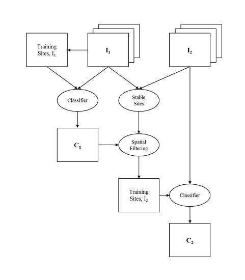
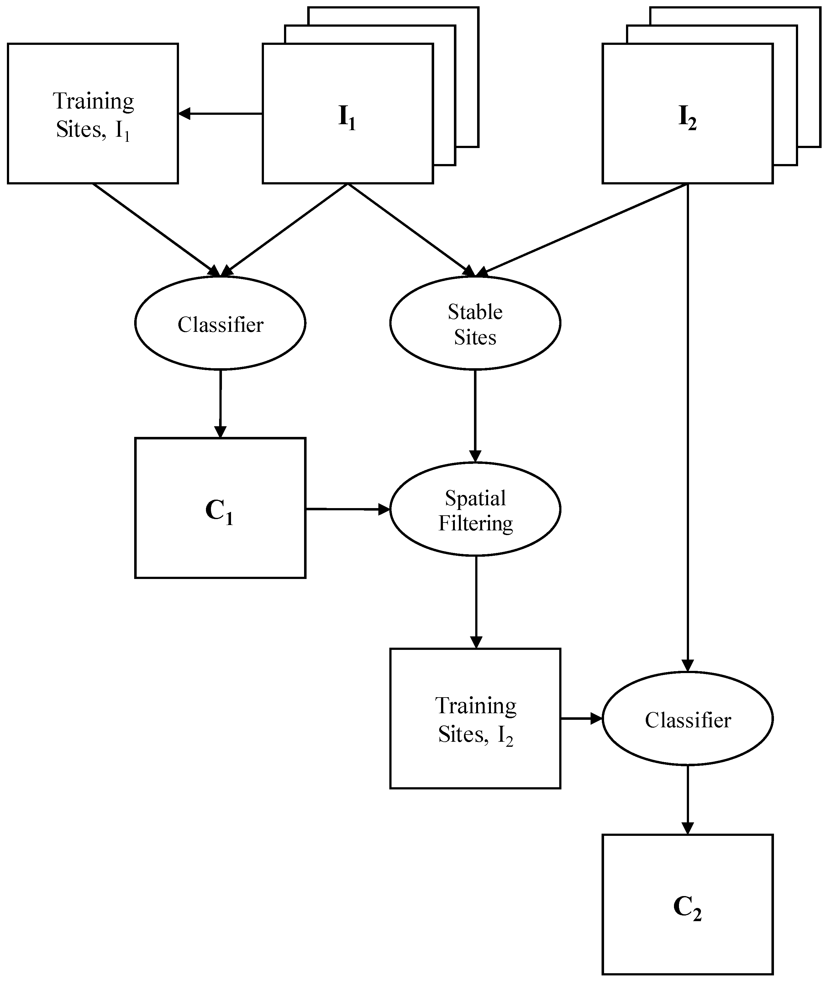
2.1. Automatic Adaptive Signature Generalization
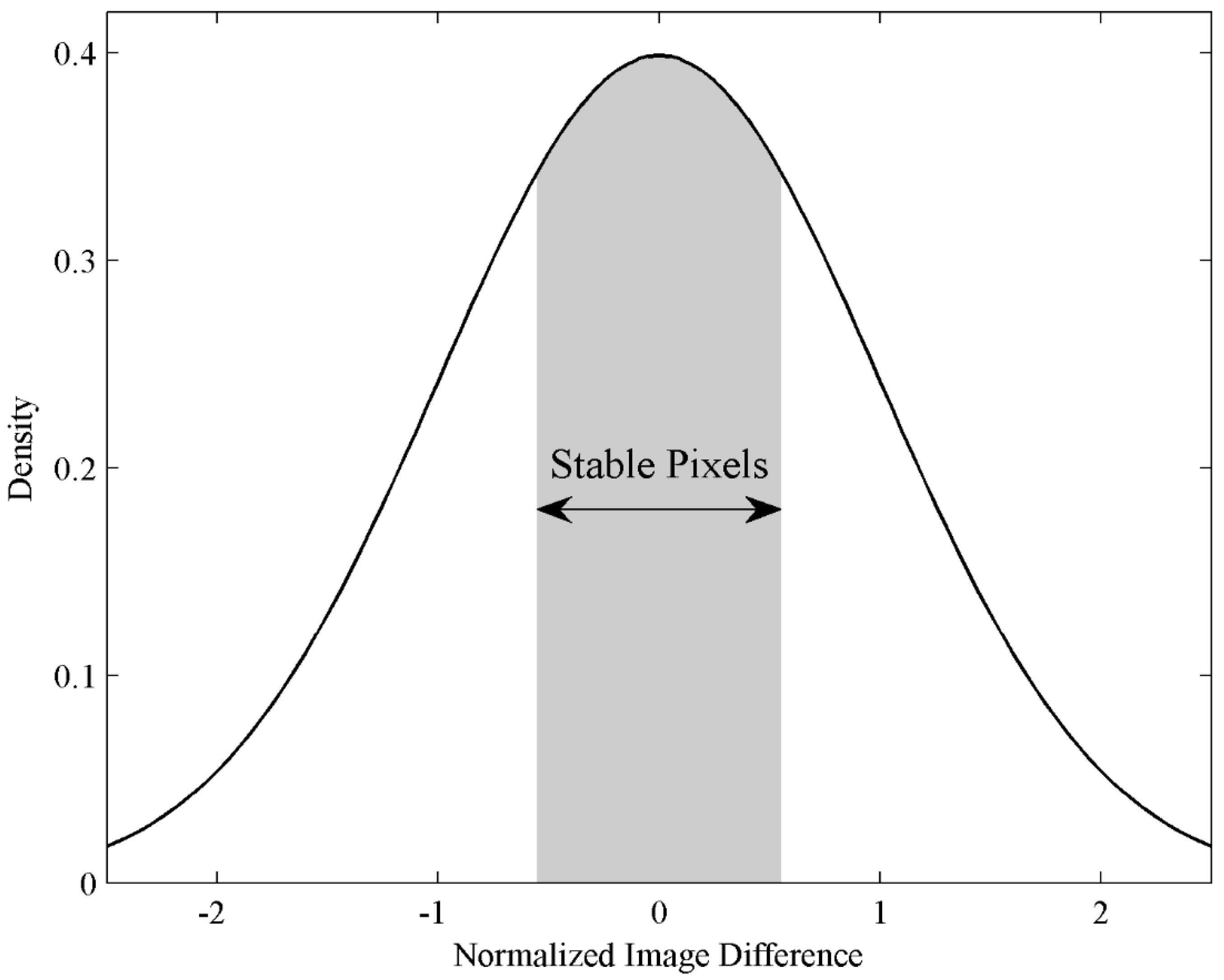
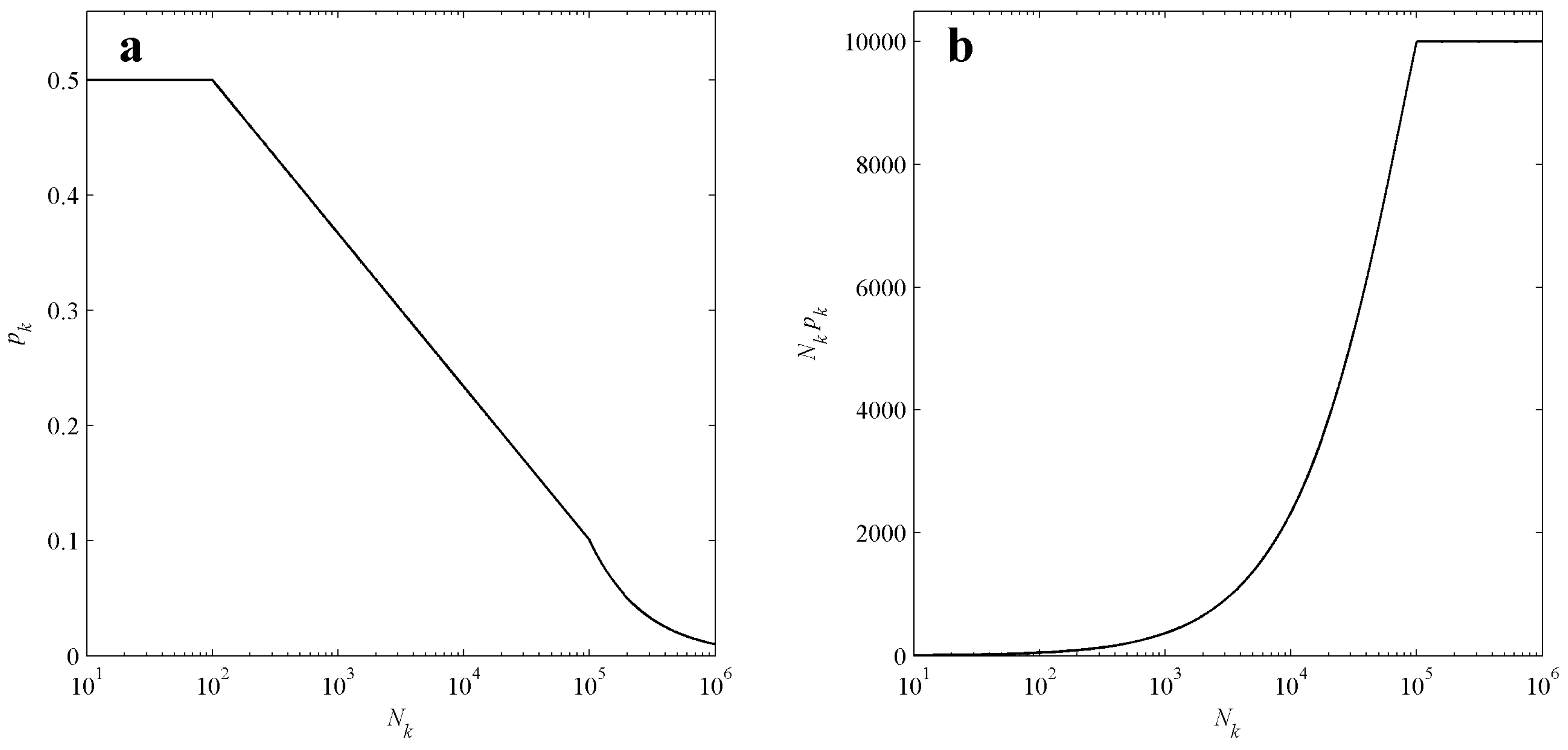
2.2. Class-Specific Thresholds for Stable Site Identification
2.3. Topographic Metrics
2.4. Multi-Season Imagery
2.5. Random Forest Classification
2.6. Study Area and Remotely Sensed Data
2.7. Analyses
3. Results
4. Discussion
5. Conclusions
Supplementary Materials
Acknowledgments
Author Contributions
Conflicts of Interest
References
- Bonan, G.B. Forests and climate change: Forcings, feedbacks, and the climate benefits of forests. Science 2008, 320, 1444–1449. [Google Scholar] [CrossRef] [PubMed]
- Bounoua, L.; Defries, R.; Collatz, G.J.; Sellers, P.; Khan, H. Effects of land cover conversion on surface climate. Clim. Change 2002, 52, 29–64. [Google Scholar] [CrossRef]
- Bronstert, A.; Niehoff, D.; Bürger, G. Effects of climate and land-use change on storm runoff generation: Present knowledge and modelling capabilities. Hydrol. Process. 2002, 16, 509–529. [Google Scholar] [CrossRef]
- Newbold, T.; Hudson, L.N.; Hill, S.L.L.; Contu, S.; Lysenko, I.; Senior, R.A.; Borger, L.; Bennett, D.J.; Choimes, A.; Collen, B.; et al. Global effects of land use on local terrestrial biodiversity. Nature 2015, 520, 45–50. [Google Scholar] [CrossRef] [PubMed] [Green Version]
- Nagendra, H.; Munroe, D.K.; Southworth, J. From pattern to process: Landscape fragmentation and the analysis of land use/land cover change. Agric. Ecosyst. Environ. 2004, 101, 111–115. [Google Scholar] [CrossRef]
- Bonan, G.B.; Oleson, K.W.; Vertenstein, M.; Levis, S.; Zeng, X.; Dai, Y.; Dickinson, R.E.; Yang, Z.-L. The land surface climatology of the community land model coupled to the NCAR community climate model. J. Clim. 2002, 15, 3123–3149. [Google Scholar] [CrossRef]
- Bonan, G.B.; Levis, S.; Sitch, S.; Vertenstein, M.; Oleson, K.W. A dynamic global vegetation model for use with climate models: Concepts and description of simulated vegetation dynamics. Glob. Chang. Biol. 2003, 9, 1543–1566. [Google Scholar] [CrossRef]
- Running, S.W.; Nemani, R.R.; Heinsch, F.A.; Zhao, M.; Reeves, M.; Hashimoto, H. A continuous satellite-derived measure of global terrestrial primary production. Bioscience 2004, 54, 547–560. [Google Scholar] [CrossRef]
- Sexton, J.O.; Urban, D.L.; Donohue, M.J.; Song, C. Long-term land cover dynamics by multi-temporal classification across the Landsat-5 record. Remote Sens. Environ. 2013, 128, 246–258. [Google Scholar] [CrossRef]
- Hansen, M.C.; Potapov, P.V.; Moore, R.; Hancher, M.; Turubanova, S.A.; Tyukavina, A.; Thau, D.; Stehman, S.V.; Goetz, S.J.; Loveland, T.R.; et al. High-resolution global maps of 21st-century forest cover change. Science 2013, 342, 850–853. [Google Scholar] [CrossRef] [PubMed]
- Loveland, T.R.; Reed, B.C.; Brown, J.F.; Ohlen, D.O.; Zhu, Z.; Yang, L.; Merchant, J.W. Development of a global land cover characteristics database and IGBP DISCover from 1 km AVHRR data. Int. J. Remote Sens. 2000, 21, 1303–1330. [Google Scholar] [CrossRef]
- Hansen, M.C.; DeFries, R.S.; Townshend, J.R.G.; Sohlberg, R. Global land cover classification at 1 km spatial resolution using a classification tree approach. Int. J. Remote Sens. 2000, 21, 1331–1364. [Google Scholar] [CrossRef]
- Friedl, M.A.; Sulla-Menashe, D.; Tan, B.; Schneider, A.; Ramankutty, N.; Sibley, A.; Huang, X. MODIS collection 5 global land cover: Algorithm refinements and characterization of new datasets. Remote Sens. Environ. 2010, 114, 168–182. [Google Scholar] [CrossRef]
- Congalton, R.G.; Green, K. Assessing the Accuracy of Remotely Sensed Data: Principles and Practices, 2nd ed.; CRC Press: Boca Raton, FL, USA, 2009. [Google Scholar]
- Song, C.; Woodcock, C.E. Monitoring forest succession with multitemporal Landsat images: Factors of uncertainty. IEEE Trans. Geosci. Remote Sens. 2003, 41, 2557–2567. [Google Scholar] [CrossRef]
- Pax-Lenney, M.; Woodcock, C.E.; Macomber, S.A.; Gopal, S.; Song, C. Forest mapping with a generalized classifier and Landsat TM data. Remote Sens. Environ. 2001, 77, 241–250. [Google Scholar] [CrossRef]
- Gray, J.; Song, C. Consistent classification of image time series with automatic adaptive signature generalization. Remote Sens. Environ. 2013, 134, 333–341. [Google Scholar] [CrossRef]
- Western, A.W.; Grayson, R.B.; Blöschl, G.; Willgoose, G.R.; McMahon, T.A. Observed spatial organization of soil moisture and its relation to terrain indices. Water Resour. Res. 1999, 35, 797–810. [Google Scholar] [CrossRef]
- Kreft, H.; Jetz, W. Global patterns and determinants of vascular plant diversity. Proc. Natl. Acad. Sci. USA. 2007, 104, 5925–5930. [Google Scholar] [CrossRef] [PubMed]
- Currie, D.J.; Paquin, V. Large-scale biogeographical patterns of species richness of trees. Nature 1987, 329, 326–327. [Google Scholar] [CrossRef]
- Wear, D.N.; Bolstad, P. Land-use changes in southern Appalachian landscapes: Spatial analysis and forecast evaluation. Ecosystems 1998, 1, 575–594. [Google Scholar] [CrossRef]
- Feng, M.; Sexton, J.O.; Channan, S.; Townshend, J.R. A global, high-resolution (30-m) inland water body dataset for 2000: First results of a topographic-spectral classification algorithm. Int. J. Digit. Earth 2016, 9, 113–133. [Google Scholar] [CrossRef]
- Ozesmi, S.L.; Bauer, M.E. Satellite remote sensing of wetlands. Wetl. Ecol. Manag. 2002, 10, 381–402. [Google Scholar] [CrossRef]
- Corcoran, J.M.; Knight, J.F.; Gallant, A.L. Influence of multi-source and multi-temporal remotely sensed and ancillary data on the accuracy of random forest classification of wetlands in northern Minnesota. Remote Sens. 2013, 5, 3212–3238. [Google Scholar] [CrossRef]
- Beven, K.J.; Kirkby, M.J. A physically based, variable contributing area model of basin hydrology. Hydrol. Sci. J. 1979, 24, 43–69. [Google Scholar]
- Band, L.E.; Patterson, P.; Nemani, R.; Running, S.W. Forest ecosystem processes at the watershed scale: Incorporating hillslope hydrology. Agric. For. Meteorol. 1993, 63, 93–126. [Google Scholar] [CrossRef]
- Emanuel, R.E.; Epstein, H.E.; McGlynn, B.L.; Welsch, D.L.; Muth, D.J.; D’Odorico, P. Spatial and temporal controls on watershed ecohydrology in the northern Rocky Mountains. Water Resour. Res. 2010, 46. [Google Scholar] [CrossRef]
- Riveros-Iregui, D.A.; McGlynn, B.L. Landscape structure control on soil CO2 efflux variability in complex terrain: Scaling from point observations to watershed scale fluxes. J. Geophys. Res. 2009, 114. [Google Scholar] [CrossRef]
- Conrad, O.; Bechtel, B.; Bock, M.; Dietrich, H.; Fischer, E.; Gerlitz, L.; Wehberg, J.; Wichmann, V.; Böhner, J. System for Automated Geoscientific Analyses (SAGA) v. 2.1.4. Geosci. Model Dev. 2015, 8, 1991–2007. [Google Scholar] [CrossRef]
- Wolter, P.T.; Townsend, P.A. Multi-sensor data fusion for estimating forest species composition and abundance in northern Minnesota. Remote Sens. Environ. 2011, 115, 671–691. [Google Scholar] [CrossRef]
- Lucas, R.; Rowlands, A.; Brown, A.; Keyworth, S.; Bunting, P. Rule-based classification of multi-temporal satellite imagery for habitat and agricultural land cover mapping. ISPRS J. Photogramm. Remote Sens. 2007, 62, 165–185. [Google Scholar] [CrossRef]
- Latifovic, R.; Pouliot, D. Multitemporal land cover mapping for Canada: Methodology and products. Can. J. Remote Sens. 2005, 31, 347–363. [Google Scholar] [CrossRef]
- Townsend, P.; Walsh, S. Remote sensing of forested wetlands: Application of multitemporal and multispectral satellite imagery to determine plant community composition and structure in southeastern USA. Plant Ecol. 2001, 157, 129–149. [Google Scholar] [CrossRef]
- Yuan, F.; Sawaya, K.E.; Loeffelholz, B.C.; Bauer, M.E. Land cover classification and change analysis of the Twin Cities (Minnesota) Metropolitan Area by multitemporal Landsat remote sensing. Remote Sens. Environ. 2005, 98, 317–328. [Google Scholar] [CrossRef]
- Breiman, L. Random forests. Mach. Learn. 2001, 45, 5–32. [Google Scholar] [CrossRef]
- Pal, M. Random forest classifier for remote sensing classification. Int. J. Remote Sens. 2005, 26, 217–222. [Google Scholar] [CrossRef]
- Gislason, P.O.; Benediktsson, J.A.; Sveinsson, J.R. Random forests for land cover classification. Pattern Recognit. Lett. 2006, 27, 294–300. [Google Scholar] [CrossRef]
- Prasad, A.M.; Iverson, L.R.; Liaw, A. Newer classification and regression tree techniques: Bagging and random forests for ecological prediction. Ecosystems 2006, 9, 181–199. [Google Scholar] [CrossRef]
- Cutler, D.R.; Edwards, T.C., Jr.; Beard, K.H.; Cutler, A.; Hess, J.G.; Lawler, J.T. Random forests for classification in ecology. Ecology 2007, 88, 2783–2792. [Google Scholar] [CrossRef] [PubMed]
- Rodriguez-Galiano, V.F.; Chica-Olmo, M.; Abarca-Hernandez, F.; Atkinson, P.M.; Jeganathan, C. Random forest classification of mediterranean land cover using multi-seasonal imagery and multi-seasonal texture. Remote Sens. Environ. 2012, 121, 93–107. [Google Scholar] [CrossRef]
- Sesnie, S.E.; Finegan, B.; Gessler, P.E.; Thessler, S.; Ramos Bendana, Z.; Smith, A.M.S. The multispectral separability of Costa Rican rainforest types with support vector machines and random forest decision trees. Int. J. Remote Sens. 2010, 31, 2885–2909. [Google Scholar] [CrossRef]
- Rodriguez-Galiano, V.F.; Ghimire, B.; Rogan, J.; Chica-Olmo, M.; Rigol-Sanchez, J.P. An assessment of the effectiveness of a random forest classifier for land-cover classification. ISPRS J. Photogramm. Remote Sens. 2012, 67, 93–104. [Google Scholar] [CrossRef]
- Wear, D.N.; Greis, J.G. The Southern Forest Futures Project: Technical Report; General Technical Report SRS-GTR-178; USDA-Forest Service, Southern Research Station: Asheville, NC, USA, 2013.
- Masek, J.G.; Vermote, E.F.; Saleous, N.E.; Wolfe, R.; Hall, F.G.; Huemmrich, K.F.; Gao, F.; Kutler, J.; Lim, T. A Landsat surface reflectance dataset for North America, 1990–2000. IEEE Geosci. Remote Sens. Lett. 2006, 3, 68–72. [Google Scholar] [CrossRef]
- Masek, J.G.; Vermote, E.F.; Saleous, N.; Wolfe, R.; Hall, F.G.; Huemmrich, K.F.; Gao, F.; Kutler, J.; Lim, T.K. LEDAPS Calibration, Reflectance, Atmospheric Correction Preprocessing Code, Version 2. Available online: http://dx.doi.org/10.3334/ORNLDAAC/1146 (accessed on 1 March 2013).
- Kauth, R.J.; Thomas, G.S. The tasselled cap—A graphic description of the spectral-temporal development of agricultural crops as seen by Landsat. In Proceedings of the Symposium on Machine Processing of Remotely Sensed Data, West Lafayette, Indiana, 29 June–1 July 1976; pp. 41–51.
- Crist, E.P.; Cicone, R.C. Application of the tasseled cap concept to simulated thematic mapper data. Photogramm. Eng. Remote Sens. 1984, 50, 343–352. [Google Scholar]
- Homer, C.; Dewitz, J.; Fry, J.; Coan, M.; Hossain, N.; Larson, C.; Herold, N.; McKerrow, A.; VanDriel, J.N.; Wickham, J. Completion of the 2001 national land cover database for the conterminous United States. Photogramm. Eng. Remote Sens. 2007, 73, 337–341. [Google Scholar]
- Fry, J.A.; Xian, G.; Jin, S.; Dewitz, J.A.; Homer, C.G.; Yang, L.; Barnes, C.A.; Herold, N.D.; Wickham, J.D. Completion of the 2006 National land cover database for the conterminous United States. Photogramm. Eng. Remote Sens. 2011, 77, 858–864. [Google Scholar]
- Homer, C.; Dewitz, J.; Yang, L.; Jin, S.; Danielson, P.; Xian, G.; Coulston, J.; Herold, N.; Wickham, J.; Megown, K. Completion of the 2011 national land cover database for the conterminous United States—Representing a decade of land cover change information. Photogramm. Eng. Remote Sens. 2015, 81, 345–354. [Google Scholar]
- Wickham, J.D.; Stehman, S.V.; Fry, J.A.; Smith, J.H.; Homer, C.G. Thematic accuracy of the NLCD 2001 land cover for the conterminous United States. Remote Sens. Environ. 2010, 114, 1286–1296. [Google Scholar] [CrossRef]
- Wickham, J.D.; Stehman, S.V.; Gass, L.; Dewitz, J.; Fry, J.A.; Wade, T.G. Accuracy assessment of NLCD 2006 land cover and impervious surface. Remote Sens. Environ. 2013, 130, 294–304. [Google Scholar] [CrossRef]
- Fiorella, M.; Ripple, W.J. Determining successional stage of temperate coniferous forests with Landsat satellite data. Photogramm. Eng. Remote Sens. 1993, 59, 239–246. [Google Scholar]
- Olofsson, P.; Foody, G.M.; Herold, M.; Stehman, S.V.; Woodcock, C.E.; Wulder, M.A. Good practices for estimating area and assessing accuracy of land change. Remote Sens. Environ. 2014, 148, 42–57. [Google Scholar] [CrossRef]
- Foody, G.M.; Cox, D.P. Sub-pixel land cover composition estimation using a linear mixture model and fuzzy membership functions. Int. J. Remote Sens. 1994, 15, 619–631. [Google Scholar] [CrossRef]
- Foody, G.M. Estimation of sub-pixel land cover composition in the presence of untrained classes. Comput. Geosci. 2000, 26, 469–478. [Google Scholar] [CrossRef]
- Atkinson, P.M.; Cutler, M.E.J.; Lewis, H. Mapping sub-pixel proportional land cover with AVHRR imagery. Int. J. Remote Sens. 1997, 18, 917–935. [Google Scholar] [CrossRef]
- Bastin, L. Comparison of fuzzy c-means classification, linear mixture modelling and MLC probabilities as tools for unmixing coarse pixels. Int. J. Remote Sens. 1997, 18, 3629–3648. [Google Scholar] [CrossRef]
- Foody, G.M. Relating the land-cover composition of mixed pixels to artificial neural network classification output. Photogramm. Eng. Remote Sens. 1996, 62, 491–499. [Google Scholar]


| Year | Season | ||
|---|---|---|---|
| Early | Mid | Late | |
| 2001 | 18 September 2001 | ||
| 2006 | 9 April 2006 | 18 August 2007 | 5 December 2006 |
| 2011 | 7 April 2011 | 10 August 2010 | 1 November 2011 |
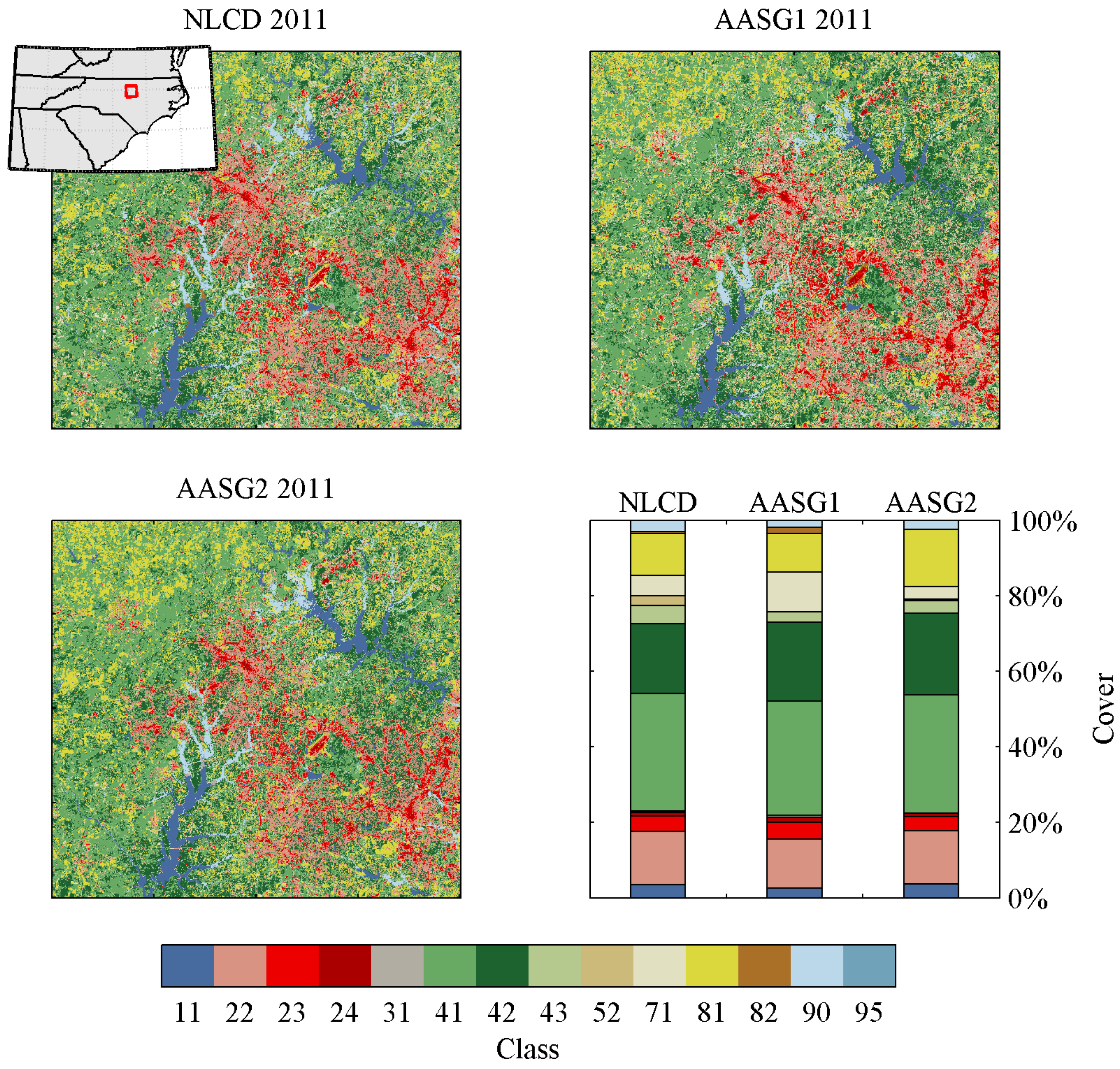
| Class | NLCD | AASG1 (OA = 60.2%) | AASG2 (OA = 70.2%) | |||||||
|---|---|---|---|---|---|---|---|---|---|---|
| Cover | Cover | PA | UA | Cover | PA | UA | ||||
| 11 | Open water | 3.4% | 2.5% | 70.4% | 97.5% | 3.6% | 89.7% | 86.9% | ||
| 22 | Low intensity developed | 13.7% | 12.8% | 63.8% | 68.4% | 13.6% | 73.0% | 73.4% | ||
| 23 | Medium intensity developed | 3.4% | 4.0% | 55.9% | 46.9% | 3.4% | 60.6% | 61.0% | ||
| 24 | High intensity developed | 0.9% | 1.3% | 57.7% | 40.5% | 0.9% | 60.3% | 61.5% | ||
| 31 | Barren land | 0.3% | 1.2% | 12.7% | 3.2% | 0.4% | 9.4% | 7.2% | ||
| 41 | Deciduous Forest | 32.5% | 29.9% | 68.0% | 74.1% | 29.6% | 75.8% | 83.3% | ||
| 42 | Evergreen forest | 18.6% | 21.3% | 69.4% | 60.8% | 21.1% | 79.5% | 70.2% | ||
| 43 | Mixed forest | 5.3% | 0.9% | 2.5% | 14.8% | 5.2% | 36.2% | 36.7% | ||
| 52 | Shrub/scrub | 1.0% | 0.1% | 0.4% | 6.2% | 0.7% | 16.7% | 23.6% | ||
| 71 | Grassland/herbaceous | 5.6% | 8.9% | 29.3% | 18.4% | 3.4% | 23.5% | 38.7% | ||
| 81 | Pasture/hay | 11.6% | 12.5% | 73.4% | 68.0% | 15.9% | 87.4% | 63.6% | ||
| 82 | Cultivated crops | 0.7% | 0.8% | 9.4% | 8.5% | 0.0% | 2.6% | 53.0% | ||
| 90 | Woody wetlands | 2.9% | 3.7% | 41.4% | 32.1% | 2.2% | 50.7% | 65.7% | ||
| 95 | Emergent herbaceous wetlands | 0.1% | 0.2% | 11.1% | 5.2% | 0.0% | 3.9% | 20.5% | ||
| Class | NLCD | AASG1 (OA = 60.1%) | AASG2 (OA = 67.9%) | |||||||
|---|---|---|---|---|---|---|---|---|---|---|
| Cover | Cover | PA | UA | cover | PA | UA | ||||
| 11 | Open water | 3.5% | 2.6% | 70.6% | 95.3% | 3.6% | 92.6% | 88.3% | ||
| 22 | Low intensity developed | 14.1% | 13.0% | 64.9% | 70.3% | 14.1% | 73.5% | 73.1% | ||
| 23 | Medium intensity developed | 4.0% | 4.4% | 54.4% | 49.8% | 3.5% | 55.7% | 62.8% | ||
| 24 | High intensity developed | 1.1% | 1.4% | 57.6% | 43.4% | 1.0% | 55.8% | 60.6% | ||
| 31 | Barren land | 0.3% | 0.5% | 6.0% | 2.9% | 0.1% | 3.8% | 12.2% | ||
| 41 | Deciduous Forest | 31.1% | 30.1% | 70.9% | 73.4% | 31.3% | 76.4% | 76.0% | ||
| 42 | Evergreen forest | 18.5% | 21.0% | 72.3% | 63.7% | 21.7% | 78.3% | 66.8% | ||
| 43 | Mixed forest | 4.9% | 2.7% | 6.6% | 12.2% | 3.3% | 22.6% | 34.0% | ||
| 52 | Shrub/scrub | 2.6% | 0.0% | 0.0% | 5.2% | 0.3% | 3.8% | 31.7% | ||
| 71 | Grassland/herbaceous | 5.4% | 10.6% | 30.0% | 15.3% | 3.4% | 19.6% | 31.1% | ||
| 81 | Pasture/hay | 11.1% | 10.3% | 66.0% | 71.4% | 15.2% | 86.0% | 62.6% | ||
| 82 | Cultivated crops | 0.6% | 1.6% | 12.0% | 4.3% | 0.0% | 2.7% | 63.9% | ||
| 90 | Woody wetlands | 2.9% | 1.9% | 31.3% | 48.3% | 2.4% | 50.7% | 60.2% | ||
| 95 | Emergent herbaceous wetlands | 0.1% | 0.1% | 4.4% | 9.7% | 0.0% | 1.7% | 41.9% | ||
© 2016 by the authors; licensee MDPI, Basel, Switzerland. This article is an open access article distributed under the terms and conditions of the Creative Commons Attribution (CC-BY) license (http://creativecommons.org/licenses/by/4.0/).
Share and Cite
Dannenberg, M.P.; Hakkenberg, C.R.; Song, C. Consistent Classification of Landsat Time Series with an Improved Automatic Adaptive Signature Generalization Algorithm. Remote Sens. 2016, 8, 691. https://doi.org/10.3390/rs8080691
Dannenberg MP, Hakkenberg CR, Song C. Consistent Classification of Landsat Time Series with an Improved Automatic Adaptive Signature Generalization Algorithm. Remote Sensing. 2016; 8(8):691. https://doi.org/10.3390/rs8080691
Chicago/Turabian StyleDannenberg, Matthew P., Christopher R. Hakkenberg, and Conghe Song. 2016. "Consistent Classification of Landsat Time Series with an Improved Automatic Adaptive Signature Generalization Algorithm" Remote Sensing 8, no. 8: 691. https://doi.org/10.3390/rs8080691