1. Introduction
1.1. Motivation for Sea-Ice Classification
Observations of recent drastic changes in the Arctic sea-ice cover have raised academic interest and public concern, motivating research that leads to an understanding of the role of the Arctic sea ice in the global system (Maslanik et al. [
1,
2], Rothrock et al. [
3], Vinnikov et al. [
4], Cavalieri et al. [
5], Serreze et al. [
6], Stroeve et al. [
7,
8], Drobot et al. [
9], Serreze and Stroeve [
10]).
The rapid decline of the Arctic sea-ice cover is one of the most obvious signs of climate change, as documented in the Fifth Assessment Report of the Intergovernmental Panel on Climate Change [
11] and one that has threatening consequences for weather, climate, ecosystems and human livelihood in the northern hemisphere (Mahoney et al. [
12], George et al. [
13], Druckenmiller et al. [
14]). Sea ice behaves as an insulator and modulates heat, moisture, and momentum transfers between the atmosphere and ocean and is both an indicator and a driver of climate change. However, even more alarming than the observed reduction in geographic extent of sea ice is the finding that the older, multi-year ice is disappearing faster than the relatively thin first-year ice (Maslanik et al. [
15]). An ice-free summer Arctic ocean is predicted to occur in 20–50 years (Jahn et al. [
16]). While a trend of rising Arctic temperatures continues, sea ice coverage undergoes large fluctuations (Serreze and Stroeve [
10]), but the fact of a long-term decrease remains.
Most large-scale studies on the variability of Arctic sea ice (Stroeve et al. [
8]) are based on estimates of the geographic extent and/or area of the Arctic sea ice cover, as derived from satellite visible/infrared imagery or passive microwave data. To better understand how and why the sea ice cover is changing, the mass balance of sea ice must be quantified, which requires measurement of sea ice thickness in addition to spatial coverage. The National Research Council, in its Decadal Survey of priorities for Earth science from space, identified estimates of sea ice thickness change as a primary objective [
17].
Direct measurement of sea-ice freeboard with a precision of a few centimeters is possible with the Geoscience Laser Altimeter System (GLAS) aboard ICESat (Kwok et al. [
18], Zwally et al. [
19]), however, these data are temporally and spatially very limited. Knowledge of the spatial distribution of leads and polynias is vital to assessing basin-wide estimates of ice thickness and mass change. Altimeter data over sea-ice have been collected in NASA’s Operation IceBridge airborne campaigns (see, e.g., Farrell et al. [
20], Kern et al. [
21]) and by European Space Agency’s CryoSat-2 (Laxon et al. [
22]). Collection of high-resolution data from unmanned aerial systems, equipped with altimeters, can provide valuable local and regional information (Crocker et al. [
23], Herzfeld et al. [
24]). Sea-ice thickness can also be estimated from Special Sensor Microwave/Imager (SSM/I) brightness temperatures, from passive microwave radiometers in general (e.g., Cavalieri [
25], Cavalieri et al. [
26], Tateyama et al. [
27], Aulicino et al. [
28]) and from L-Band brightness temperature observations (1.4 Ghz) collected by the Microwave Imaging Radiometer using Aperture Synthesis (MIRAS) during ESA’s Soil Moisture and Ocean Salinity (SMOS), but only for thin and not melting ice (Kaleschke et al. [
29,
30]).
The work in this paper is motivated by the facts that older, thicker ice is typically less susceptible to melting as well as morphologically more complex than younger ice (Herzfeld et al. [
31]), and hence mass loss may not be directly derived from freeboard and area of coverage. We introduce an approach to spatial classification from SAR data to discern properties and provinces of Arctic sea ice as a means to understand and manage this complexity and its relevance to Arctic change.
As the sea ice is highly heterogeneous in the Arctic Ocean in its entirety as well as in smaller provinces and at each scale constantly changing, mapping and understanding characteristic properties and morphogenetic, kinematic and dynamic processes become important. With the availability of high-resolution Synthetic Aperture Radar (SAR) data (e.g., 12.5 m for RADARSAT-1), such investigations also become possible. SAR data are useful for investigations of Arctic sea ice, because the SAR signal penetrates the cloud cover that is often present in the Arctic, and because they have a high spatial resolution. SAR data have been collected by RADARSAT-1, RADARSAT-2 (Canadian Space Agency and NASA), ERS-1, ERS-2 and ENVISAT (European Space Agency (ESA)) and JERS (Japanese Space Agency) satellites, and recently by SENTINEL-1 (European Commission’s Earth Observation Programme “Copernicus” ).
1.2. Requirements for Sea-Ice Classification Methods for SAR Data and an Avenue for a Solution
A problem that indicates a need for sea-ice classification is that multi-year sea ice, which has been identified as a major source of ice loss (Maslanik et al. [
15]), typically has a complex morphology (Herzfeld et al. [
31]). Other needs of sea-ice classification lie in sea-ice forecast related to marine shipping routes (see, e.g., Karvonen et al. [
32]), and in understanding the stability or the danger of potential instability of shorefast ice for inuit hunters (George et al. [
13], Druckenmiller et al. [
14]). The Canadian Ice Service employs thickness-redistribution functions in its forecasting models (e.g., Savage [
33], Kubat et al. [
34,
35,
36,
37]. The problem of complexity relates to ice transport, ridging and other forms of deformation, which on the modeling side is treated in Harder and Lemke [
38], Hunke [
39], Hunke et al. [
40], Steiner et al. [
41], Bourke and Garrett [
42] and Flato and Hibler [
43]. These applications call for a data analysis method that can identify complex processes and properties in the sea ice. The objective of this paper is to introduce an approach that allows to derive such information from Synthetic Aperture Radar (SAR) data. Radiation at microwave wavelengths easily penetrates clouds and darkness, making radar sensors ideal for observing the polar regions. In addition, SAR sensors have very high spatial resolution, typically on the order of tens of meters (12.5 m for the RADARSAT high-resolution product used here), and respond to surface roughness and internal ice properties such as salinity and the presence of volume scatterers (Onstott [
44]).
Analysis and classification of sea ice from SAR data has been a topic of increasing research in the past year to two decades. A summary of approaches and comparison to the method derived in this paper is given in the discussion section (
Section 11), because it is most useful to the reader after the introduction, application and validation of the method derived here.
As motivated above, the objective is to derive a method for automated sea-ice classification from SAR data that identifies spatial properties and classes that are linked to physical properties or are indicative of physical processes that the sea ice has experienced (morphogenesis). A new approach is required to achieve this classification objective from SAR data because of the following limitations. The fact that most SAR data are single-channel data renders the largest class of image classification methods useless, which is the class of multi-variate statistical methods. Segmentation based on backscatter values (grey values) is ambiguous for SAR data, since many examples can be found of characteristically different ice classes which have similar grey values but different spatial characteristics and represent different ice types. For instance, open water and very smooth ice may have a similar signature in SAR data, but on the other hand wind-roughened open water will have a higher backscatter value than calm open water. In consequence, analysis of spatial patterns of SAR values in a neighborhood or window is required to distinguish more than a few property classes. Realizing that a limitation of many image processing methods lies in the small window sizes, we will utilize mid-sized moving windows which capture the spatial characteristics of sea-ice types. The principal idea in our classification method is to exploit the spatial structure of sea-ice properties, as reflected in SAR data.
The geostatistical classification method that will be utilized in this paper is motivated by concepts of structural mechanics. Spatial statistics will then be applied to identify spatially repeating patterns in data sets and associate characteristic parameters. This has been demonstrated for deformation states in surge glaciers (Herzfeld and Zahner [
45], Herzfeld et al. [
46]) but not been applied to sea-ice deformation. In the first part of the paper, we will establish a similar approach for characterization of sea ice and parameterization of sea-ice types.
The next goal is to derive an approach to sea-ice classification. We noted that multivariate statistical methods cannot be directly applied to single-channel data such as SAR data. However, if we can create a multi-component vector field from the original SAR data set, then such multi-variate methods will become applicable again. This will be addressed in the second part of the paper, combining geostatistical feature vectors and multi-variate statistical classification techniques (supervised and unsupervised classification). The methods and algorithms are implemented as part of the software package libgeoclass by U.C. Herzfeld and S. Williams.
In applications to RADARSAT data and ERS-2 SAR data from the region near Point Barrow, Alaska, we will demonstrate that the implicit analysis of spatially repeating patterns lends itself to discriminating different sea-ice types in both shore-fast ice and near-shore pack ice. The methods will be validated using field and aerial observations.
2. Concepts and Mathematical Principles of the Geostatistical Classification Method
2.1. Objectives of Classification
The method presented here to extract information from RADARSAT SAR data and identify sea-ice provinces and properties is an image classification method. The objective of classification is to explore given properties of an image or a data field and extract characteristics that allow for the association of defined classes of objects. Association is a complicated highly nonlinear operation and as such necessitates the development of computationally efficient algorithms. The challenge is then to retain and capture the salient information in the image or data set.
An approach commonly used in classification of remote sensing data is the application of classification algorithms based on moving windows operating on small neighborhoods, typically 3 × 3, 5 × 5 or 7 × 7 pixels, or templates of pixel patterns in small neighborhoods. The disadvantage of this alternative is that intermediate and large-scale features are not captured in the analysis, and that the use of templates in classification may induce a pattern similar to that of the template. For instance, if isotropic templates are used then the algorithm often gives a preference to isotropic structures (as e.g., in Caers [
47]). At the other extreme, utilizing an entire image at once in training a classification method is not only computationally prohibitive, but also results in overtraining of the classification algorithm, as too many unnecessary details in the training image will be retained.
An additional challenge in designing a classification method for Synthetic Aperture Radar (SAR) data is that SAR data lack absolute reference, both in scale and radiometric value, and depend on look-angle. Classification based on data with lack of absolute reference requires mathematical methods that do not depend on absolute values but on first-order differences.
In summary, automated classification based on SAR data requires the design of an algorithm that
captures the salient information
reduces the total data volume and the number of required operations,
utilizes mathematical methods that do not depend on absolute values but on first-order or higher-order differences, and
is sensitive to anisotropies.
Our solution utilizes a moving-window technique with intermediate-sized windows, the determination of the window size is described below in connection with the concepts of
homogeneity and
sea-ice provinces. To meet the requirements (1) and (2) of data reduction and operationality of the algorithm and at the same time capture the intermediate-scale information contained in each window, spatially and directionally dependent functions are calculated for each window, and then parameters are extracted from those functions and employed to build up a feature vector. We use
vario functions as introduced in Herzfeld [
48] to meet requirement (3) and calculate them for several directions for each window to meet the anisotropy requirement (4).
Several alternative approaches may lead to class association:
- (a)
The classification is based on association of a class (here: a sea-ice class) to a feature vector, each class is color coded in an output image.
- (b)
A parameter map is stored for each parameter that is extracted from the directional vario function. The parameter map represents a characterization of sea-ice properties.
- (c)
The entire SAR data set/image is segmented into sea-ice provinces, using a classification based on a combination of parameter maps.
- (d)
A neural network is trained for class association, based either on vario functions or on feature vectors, and applied for each window.
Class association using a deterministic function based on feature vectors as in approach (a) was used for seafloor classification in Herzfeld and Higginson [
49]. The sea-floor classes are in essence (1) submarine volcanoes (round, near isotropic); (2) mid-atlantic-ridge flank regions (highly anisotropic sequences of ridges and valleys, very rough morphology) and (3) sediment ponds (flat regions with smooth surfaces). Because the sea-ice morphology in the study area off Point Barrow, Alaska, is spatially much more complex than the sea-floor morphology in the region of the Atlantic investigated in Herzfeld and Higginson [
49], it is hard to establish a deterministic function that will serve to separate sea-ice surface classes based on feature vectors. Therefore in this paper we will take an approach that combines methods (b) and (c). First, maps of characteristics parameters will be calculated (approach (b)). This characterization approach works for any surface of any complexity. Building on the results of (b), further classification of sea-ice provinces can be carried out by application of existing unsupervised or supervised classification algorithms. In the case studies presented in this paper, we will follow approaches (b) and (c) and demonstrate that classification of sea-ice types and segmentation of the regions near Point Barrow into sea-ice provinces is possible. An example of approach (d) is the connectionist-geostatistical classification derived and applied in Herzfeld and Zahner [
45] for classification of crevasse patterns in a surging glacier (Bering Glacier, Alaska). For sea-ice-data analysis this is work in progress.
2.2. Definitions
2.2.1. Spatial Surface Structure and Vario Functions
We analyze the
spatial surface structure of sea ice in the form in which it is reflected in SAR data. Formative processes (kinematic and dynamic processes and environmental processes such as snow fall, melting, wind erosion and deposition) that affect the morphology of the surface are captured in differences of surface values. If we are interested in characterizing the surface structure of a given area, then averages of such differences formed over the same distance (or distance and direction) will contain the essential information. Mathematically, we form
for pairs of points
, where
is an observation of the variable
z at location
,
is a region in
(case of survey profiles) or
(case of survey areas) and
n is the number of pairs separated by
h; the distance value
h is also termed “lag” (∈ - element of;
-two- and three-dimensional space of real numbers (coordinates), respectively). The function
is called the
first-order vario function. This function exists always and has a finite value, because only finitely many data points enter the calculation.
The first-order vario function is numerically equivalent to the variogram, provided that the data may be considered a realization of a spatial stochastic process that satisfies the intrinsic hypothesis (see Herzfeld [
48]). The vario function, however, has the advantage that it may be calculated for any discrete data set and also generalized to higher order. The place of the intrinsic hypothesis condition is, in a way, taken by the homogeneity condition. The reader interested in the background and philosophy of various mathematical theories and their application to geophysical data may be referred to Herzfeld [
48], Luenberger [
50], Grafarend [
51], Journel [
52], Matheron [
53], Herzfeld [
48,
54]. The reader who is mainly interested in the SAR classification method may simply keep in mind that an objective function is calculated for each window and each direction, from which well-defined parameters are being extracted for classification purposes. The geostatistical classification method is more mathematically and more comprehensively introduced in Herzfeld [
55].
2.2.2. Spatial Surface Roughness
The concept of spatial surface structure is closely related to that of spatial surface roughness. Surface roughness is defined as the spatial derivative of surface elevation. Morphologic properties at any scale are not captured by absolute elevation (above an imaginary zero reference, such as sea level) but rather by changes of elevation in space. At larger scale this is topographic relief, at small scale roughness. For instance, spatial ice surface roughness is a morphologic characteristic of ice surfaces. (Note that the convention of large scale for low resolution and small scale for high resolution is used herein, which is opposite to the convention used in cartographic scale.)
Using this definition, surface roughness contains the complete morphologic information of the surface under study. This may sound trivial, but in some disciplines surface roughness is commonly understood as roughness length, a one-dimensional parameter, or root-mean-square roughness, a one-dimensional statistical approximation. For instance, aerodynamic roughness (length) is used in meteorology (e.g., Oke [
56]). However, roughness length can be derived from (spatial) surface roughness (see
Section 5 and Herzfeld et al. [
31]).
2.2.3. Characterization—Classification—Segmentation
The objective of (mathematical) characterization is to determine a set of parameters that uniquely describe an object. The objective of classification is to associate a given object to one of a number of classes; so that the class association can be carried out for each case automatically, a rest class may be required to collect all objects that do not belong to any of the characteristic classes, depending on the class association method. In each new application, the characterization problem must be mastered before the classification problem. By moving a classification operator over a large spatial data set, such as an image, each window is associated to a class, and a segmentation may be achieved. A segmentation into reasonably coherent subsets or segments may require smoothing; however, in a good classification this is not necessary (see Herzfeld and Higginson [
49] for examples and details). Case studies (1) and (2) will be examples of characterizations, and case studies (3) and (4) will be examples of classifications and segmentations of SAR data sets into sea-ice classes.
2.2.4. Concept of Homogeneity
Extraction of parameters that are characteristic of an area requires the concept of homogeneity: An area is called homogeneous with respect to surface structure if the area has the same surface structure throughout, but the structure may be complex and resulting from several morphogenetic events, phases, or processes, as long as all those processes have affected the entire area in the same way. The term heterogeneous is reserved to mean “not homogeneous".
In view of data analyses, one needs to notice the following borderline cases: Assume two different patterns, A and B. If an area is 20 m long with 10 m of pattern A and 10 m of pattern B, then the area is heterogeneous. If a second area is 100 m long with patterns A and B alternating every 10 m, then the area is called homogeneous. This should be considered when selecting optimal window sizes in classification, as the window size needs to be large enough to contain at least two repetitions of the largest characteristic features.
2.2.5. Terminology for Classification: Sea-Ice Type, Sea-Ice Class and Sea-Ice Province
Colloquially, we use the term
sea-ice type to distinguish for instance heavily rubbled and ridged ice, smooth sea ice, very smooth sea ice, young sea ice and old sea ice. Images of deformed ice, in particular of ridges and rubble fields, are given in Tucker et al. [
57], Steffen [
58].
A sea-ice class is a type of sea ice that is uniquely characterized by its structural properties and distinct from all other classes. In a first example, the goal may be to map areas of smooth ice versus areas of rough ice. This can be achieved through a classification with two classes, (1) smooth ice; (2) rough ice (everything that does not satisfy our criterion for smooth ice). In a second example, we may want to distinguish more types of rough ice, which may lead to a classification with 5 classes (1) smooth ice; (2) ice with rubbles and ridges to 10 m diameter; (3) ice with rubbles and ridges larger than 10 m diameter; (4) smooth ice areas broken up by leads; (5) other complex ice areas.
A
sea-ice province is an area of sea ice that is homogeneous with respect to the sea-ice classes it contains. The ice in a province has experienced the same morphogenetic, kinematic and dynamic processes. For instance, a connected area of smooth sea ice containing ice that has just formed may be considered a province. A province in the Beaufort Sea offshore of Point Barrow may contain heavily ridged and rubbled ice with faulted and overthrust ice sheet segments, interspersed with smooth areas that have formed when open water areas between faulted blocks froze over again (see, Section (3) and Herzfeld [
55]).
3. Vario Parameters and their Role in the Geostatistical Classification Method
3.1. Mathematical Introduction of Vario Parameters
Different parameters have been defined in a suite of geophysical studies (see e.g., Herzfeld and Higginson [
49], Herzfeld [
59], Stosius and Herzfeld [
55,
60]). In the following analysis of SAR data, we employ the parameters
,
,
and
, which are illustrated in
Figure 1.
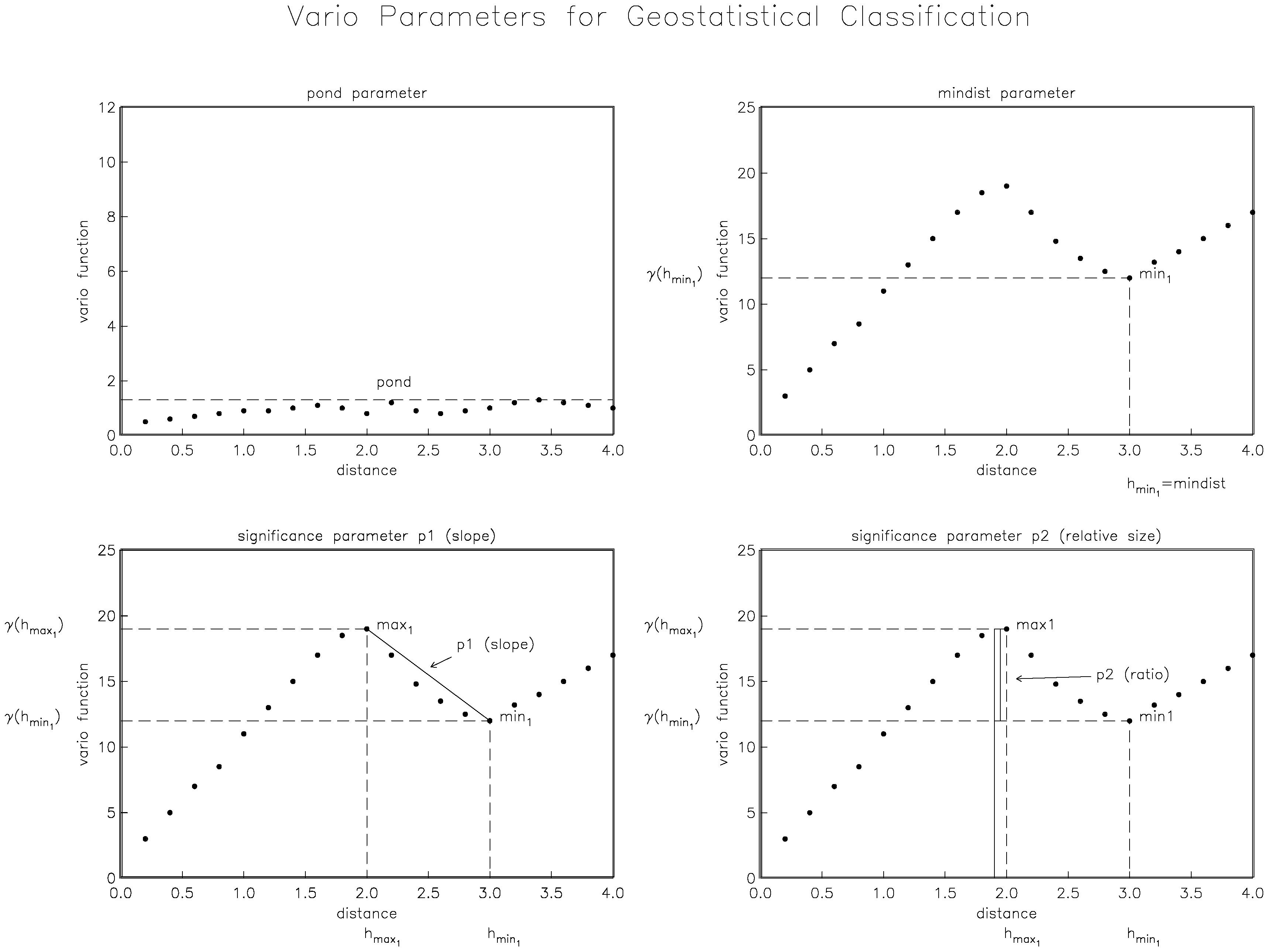
A simple, but very useful parameter is the parameter, defined as the maximum value of the vario function (in the window); it relates to total variance. If the main variable is elevation, then the parameter is directly related to surface roughness length and may be used to distinguish smooth areas from areas with morphologic relief. For reflectance values as in SAR data, the parameter depends on elevation variability, on material changes and changes in other reflective properties with distance.
The parameter
, defined as the lag of the first minimum after the first maximum in the vario function, gives the characteristic spacing of dominant surface features such as ridges, leads, or smooth frozen areas separating rubbled and ridged areas (Herzfeld et al. [
59], Herzfeld [
31], Herzfeld and Mayer [
55]).
As a background example, the vario function of an evenly-spaced hill-and-valley profile in topography is a sinusoidal wave. The lag to the first minimum in the sine curve is the characteristic spacing of hills and valleys in the topographic relief. If more than one process has affected a surface, creating a complex surface structure, the same principles still apply, but more minima and maxima in the vario function need to be utilized, and more complex parameters derived to capture enough information in the feature vector to allow a classification.
To distinguish primary features from superimposed ones, or more generally characterize more complex spatial structures, significance parameters are introduced:
is the slope parameter and
the relative significance of the first minimum
after the first maximum
, and
and
denote lag and vario-function value of
x, respectively (Herzfeld [
55]). In this notation,
Parameters
and
provide information on the significance of the spatial features whose sizes are quantified by
. For more minima and maxima,
-type parameters and
-type parameters are defined analogously. Slope parameters (
-type parameters) involve distance. Relative significance parameters (
-type parameters) are independent of dimensions and thus facilitate comparison between data from different instruments and of different scales, for example, surface roughness from satellite SAR data may be compared directly to surface roughness from Glacier Roughness Sensor (GRS) data collected in the field (Herzfeld et al. [
61]), or to other field data as will be applied in this study (see, Herzfeld et al. [
31]).
Looking in the other direction along the range of scales, parameter and related -type parameters may facilitate use of SAR data for sub-scale studies of lower resolution satellite data.
3.2. Steps of the Geostatistical Classification Method
The geostatistical classification method proceeds by the following steps:
a window is selected from the study area; this may coincide with the entire study area,
statistical or analytical spatial functions are calculated from data in the window (e.g., experimental variograms, directional vario functions of first or higher order, other functions),
spatial functions from (2) may be filtered,
parameters, called vario parameters or geostatistical classification parameters, are calculated from the functions in (2) or (3),
a feature vector is composed of the parameters,
a deterministic discrimination algorithm or connectionist class association or a statistical classification algorithm is applied to the feature vector to relate the structures in the window to an object class.
In the Barrow area sea-ice applications, multi-variate statistical methods will be used for supervised and unsupervised classification in step (6).
4. Geographical Area, Data and Sea Ice Classes
4.1. Geography of the Study Area
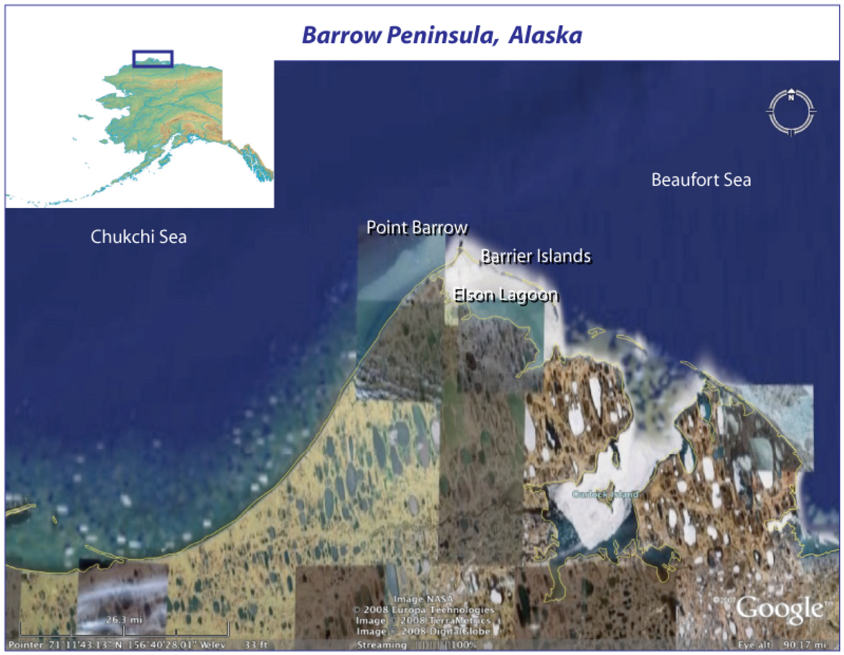
The area around Point Barrow, Alaska, has the advantage that several sea-ice types are encountered in its close vicinity in the Chukchi Sea, the Beaufort Sea, and in Elson Lagoon (see
Figure 2), comparative to sea-ice conditions found in pack ice areas several hundred kilometers further North as well as in other shore-fast areas in the Arctic. The tip of a spit at Point Barrow marks the longitudinal boundary between the Chukchi Sea in the West and the Beaufort Sea in the East. Different wind and ocean current conditions exist in the Chukchi Sea and the Beaufort Sea (cf.
Figure 3c).
The sea-ice provinces described in the sequel can be identified in the target image for classification (
Figure 3c) and in the ERS-2 data set (
Figure 4). The spit and a line of barrier islands, which extend east-southeast from Point Barrow, separate two different environments, (1) the open waters of the Beaufort Sea exposed to storm, waves and ocean current; and (2) the more protected waters of Elson Lagoon. Consequently two distinct sea-ice regimes reflect the quiescent nature of the lagoon (in (1)) and the dynamic interactions of the barrier islands and sea pack drifting on relatively shallow ground in the near-shore section of the Beaufort Sea (2). The latter creates large ridges close to shore (see inset photographs in
Figure 3b). While the snow-covered sea ice in Elson Lagoon appeared homogeneous to people working in the field in March 2003 (time of photographs), Elson Lagoon does de facto encompass several structural subregions (cf. Herzfeld et al. [
31]), which have been identified in field data and aerial passive microwave data (Polarimetric Scanning Radiometer (PSR) data, Piepmeier and Gasiewski [
62]). Sea-level change, local grounding and thermal cracking have lead to locally specific morphogenetic changes in the ice pack. Elson ice also reflects variations in ice conditions that occurred during the early stages of freeze-up, including the effect of currents flowing through the gaps between the barrier islands.
Sea ice in the Beaufort and Chukchi sea parts of the study area is morphologically complex, with ridges of several meters height and rubble fields composed of smaller and larger particles. Close to shore on the Chukchi side of the Barrow region is an area of extremely smooth ice (light blue in
Figure 3d) that is protected by a complexly ridged zone from open ocean dynamics. The complexly ridged zone is termed “stamukhi” zone (a local term, explained in the next paragraph). These two zones are known to Barrow locals to form every year, and the smooth ice is very young ice, the youngest in the study area, in March 2003 (and definitely first-year ice). Beaufort ice in the study area was found in snow-depth analyses to be organized at large scale with large ridges spaced at an average distance of 210 m, and highly ridged and rubbled in between (Herzfeld et al. [
31]. Both Chukchi ice and Beaufort ice are directionally anisotropic.
In the Chukchi Sea and the Beaufort Sea, heavily ridged and rubbled ice forms at the seaward edge of the grounded portion of the shore-fast ice, this is termed “stamukhi zone”. A stamukhi zone consists of thick ridges that become grounded during the winter and become part of the fast ice zone; while the rest of the fast ice melts during the summer, a stamukhi remains attached to the ocean bottom throughout the summer. In the Chukchi Sea sector, the stamukhi zone protects an area of very smooth ice. Seaward of the stamukhi zone is the pack ice. Ice floes of variable shapes and sizes move within the pack ice. More rounded shapes are indicative of older ice (which could still be first-year ice, cf. Maslanik et al. [
63]). At Point Barrow, ice in floes develops shear zones that lead to striata following the current off the point. Even in mid-winter, the pack ice tends to be in motion. Hence the ridged zone closest to shore is grounded, whereas the outer ones are moving. The floes shearing off of Point Barrow can be identified in the RADARSAT and ERS-2 SAR data (see
Figure 3). The area SW of the Lagoon and SE of the western coast is tundra with approximately oval-shaped lakes, remnant of subglacial movement during the time when the area was covered by inland ice.
In our analyses, we will utilize the concept of a province, akin to its use in structural geology, to identify an area homogeneous with respect to morphogenetic processes and material type (but different from a neighboring province; i.e., provinces are typically marked by clear boundaries). This will facilitate the description of the classification and its interpretation. Several provinces can be identified in
Figure 3c, where sea-ice types are indicated. A province can contain several sea-ice types, such as ridges and smooth areas in the near-shore Beaufort sea, or have subprovinces. For instance, Elson Lagoon may be considered one province, or five different provinces at closer scrutiny (Herzfeld et al. [
31]).
4.2. In-Situ Observations and Related Data Analysis Resultant from the 2003 and 2006 AMSR-E Validation Campaigns for Sea-Ice Products
Extensive field work has been conducted in the Barrow area (e.g., George et al. [
13], Eicken et al. [
64], Druckenmiller et al. [
14]), including collection of snow depth data, laser profilometer data and other aerial observations as part of the NASA AMSR-E validation campaigns for sea ice products in March 2003 and 2006, AMSRIce03 and AMSRIce06 (see Herzfeld et al. [
31], Maslanik et al. [
63], Cavalieri et al. [
65], Sturmet al. [
66], Markus et al. [
67], Heinrichs et al. [
68], Rivas et al. [
69], Stroeve et al. [
70]).
The in-situ snow depth, ice thickness, snow and surface roughness and topography data acquired during the AMSRIce03 and AMSRIce06 field experiments that are relevant to this paper are described in detail in Maslanik et al. [
63], Sturm et al. [
66] . We summarize the methodology and data briefly here. Both experiments were carried out in March, for three weeks in 2003 and one week in 2006. The in-situ observation program was combined with NASA P-3 aircraft overflights and coordinated with satellite coverage. Detailed sets of snow and ice measurements were acquired along a series of walked transects across the shore-fast ice and extending onto pack ice. Snow measurements include snow depth, density, water equivalent, stratigraphy, and grain size. Snow depths were measured using a hand operated self-recording snow depth probe, equipped with GPS, with sub-centimeter depth measurement accuracy. These measurements were taken at 0.5 m spacing along 100 m sections, with 15 such sections sampled. Depth was also measured using the same instrument at approximately 4 m spacing along transects ranging from 2 to 5 km in length. Ice thickness was measured at intervals along the transects at 25 locations. Thicknesses were also obtained using an EM-31 electromagnetic inductance instrument towed along the surface, over the same transects used for the snow depth measurements and with similar spatial sampling. During AMSRIce03, the snow depth and ice thickness observations were obtained for over a total of 18 km. Snow stratigraphy was studied using snow pits dug along the transects, while surface roughness was measured using a laser level with range pole and measuring tape. For AMSRIce03, the surface-measured roughnesses were augmented by interpretation of mosaics of high-resolution aerial photographs acquired at low altitude from a Cessna 185 aircraft. The low sun angles and excellent lighting conditions helped to highlight the variations in surface topography over the ice cover. In both experiments, field notes and ground-based photographs were acquired to help put the measurements into context. Additional details as well as field data and NASA aircraft imagery and flight tracks are available at the National Snow and Ice Data Center (
http://nsidc.org/data/amsr_validation/cryosphere/amsrice03/index.html and
http://nsidc.org/data/amsr_validation/cryosphere/amsrice06/index.html, and at
http://polynya.gsfc.nasa.gov/seaice_arctic2006.html).
Maslanik et al. [
63] provide manual classification maps based on PSR data (
Figure 3 in Maslanik et al. [
63]), this matches the target map of sea-ice types (
Figure 3d) in this paper. PSR data provide information on sea-ice roughness, using unsupervised clustering of several channels of the PSR signal. Surface roughness length derived from Airborne Topographic Mapper (ATM) data is less conclusive. Algorithms for ice-edge detection are described in Heinrichs et al. [
68] and applied to MODIS and RADARSAT data from the Barrow area. Rivas et al. [
69] study the influence of sea ice roughness on airborne lidar signals.
Geostatistical classification using hyperparameters is applied to analyze snow-depth data on sea ice in Herzfeld et al. [
31]. Results include a quantitative characterization of sea-ice provinces from field transects in the Beaufort Sea, Chukchi Sea, and Elson Lagoon, which represent a good subset of Arctic sea-ice types, an internal segmentation of the longer profiles, and a derivation of surface roughness length and of sea-ice-type complexity. PSR data reflect complexity of spatial snow depth structures as captured in multi-dimensional feature vectors, and, less directly, snow-depth and surface roughness length.
4.3. SAR Data and Derivation of Target Maps of Sea-Ice Classes
SAR data have been selected for the investigations in this paper to match the time frame of the AMSRIce03 experiment and, approximately, the AMSRIce06 experiment. We use two data sets: (A) RADARSAT SAR data from March 2003 and (B) ERS-2 SAR data from December 2005.
4.3.1. RADARSAT SAR Data
The Canadian Space Agency’s RADARSAT-1 operates a SAR in C-band at 5.3 GHZ with a bandwidth of 30 MHz and a single polarization (HH), an aperture length of 15 m and an aperture width of 1.5 m. RADARSAT-1 flies at an altitude of 793–821 km with and inclination of 98.6 in a sun-synchronous orbit, collecting at 14.29 orbits per day. It has several different beam modes.
The radar signal used in RADARSAT-1 SAR data penetrates the dry part of the snow layer that may potentially cover sea ice and reflects off the surface of the ice. Water lenses or wet snow may affect the SAR’s ice-surface retrieval capability, however, these are not likely present in March in the Arctic. A 400 by 400 pixel RADARSAT SAR data set with a pixel size of 75 m, extending 30 km east-west and 30 km north-south around Point Barrow, has been selected for this study (see,
Figure 3). The data set was collected in March 2003, at the same time as field and aerial experiments in the study area.
The SAR image (
Figure 3a) shows the western coastline and the spit running NE from lower left center to the middle of the image and turning east-southeast at the point (Pt Barrow). Elson Lagoon can be identified visually. East of the western coastline and south of Elson Lagoon is an area of tundra with frozen lakes (see also
Figure 2).
4.3.2. Derivation of Target Map of Sea-Ice Types from March 2003 RADARSAT Data
A target and validation basis is created for the classification (
Figure 3c), utilizing a SAR data set, the Google satellite image composition in
Figure 2 and expert knowledge based on field experience/observations and interpretation of field data and PSR data (Maslanik et al. [
31], Herzfeld et al. [
63]). Tendentially, open water and thin new ice (as occurs near the western coast) appear darker because of the low radar backscatter, while thicker, rougher ice appears in lighter shades of grey, due to higher backscatter. Expert knowledge is needed to derive the target classification proxy that is superimposed on the SAR data set, since a visual interpretation of SAR data would be ambiguous. Similar grey values occur in different zones of sea ice identified in
Figure 3c, whereas different spatial patterns indicate different ice types. This hints at the necessity of an automated classification employing spatial characteristics, rather than grey values (backscatter values). Ice in the Beaufort sea is highly anisotropic, according to roughness analysis from snow-depth data, this anisotropy is visible in the SAR data. Sea-ice areas identified in the image have been described in
Section 3.1.
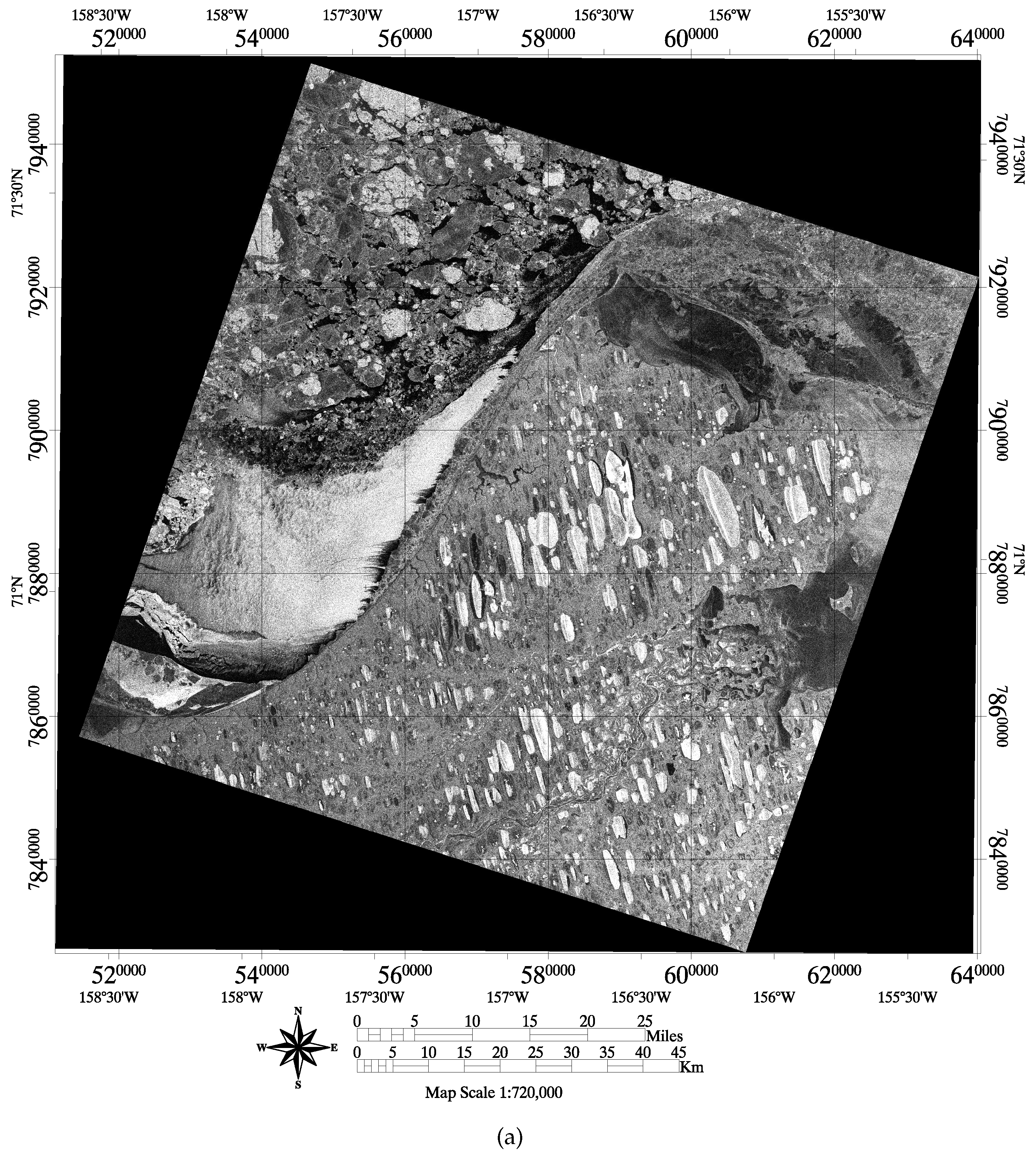
4.3.3. ERS-2 SAR Data
For applications (A.2) and (A.3) we analyze a higher-resolution SAR data set from European Remote Sensing satellite ERS-2 (E255809271G15003), which is a full-resolution image (resolution = 12.5 m) and has been collected on 22 December 2005 at 22:03:41.021 UTC. This data set is used in the form of a calibrated image with floating-point values with backscatter given in dB. The data set has been georeferenced, using UTM zone 4 (floating-point GEOTIFF E255809271G15003-warp-rectified.tif, processed by John Heinrichs, Fort Hays State University). The data set covers an area of approximately 97.2 km (y-axis) by 100.1 km (x-axis). The area in
Figure 4a,b is 128.16 km E-W by 123.48 km N-S (including the black region that is the result of georectification) The SAR sensors aboard European Remote Sensing Satellites ERS-1 and ERS-2 are essentially the same, operating in C-band (5.6 cm wavelength, frequency 5.3 GHz) and using a single polarization (VV).
In the parameter calculation, the image was used at a reduced spatial resolution of approximately 121 m by 121 m, with 1055 rows (in 128.16 km E-W) and 1024 columns (in 123.48 km N-S). The reduction in spatial resolution is a result of a format preprocessing and of course saves computational cost, while the capacities of the approaches can be demonstrated. A parameter map at window size 20, step size 1 has 1005 rows and 1036 columns, and hence each point is derived from a 2420 m by 2420 m window, where neighboring windows overlap as much as possible (step size 1 pixel width, equal to 121 m). To focus on sea-ice classification, the land ice region is masked.
4.3.4. Interpretation of ERS-2 SAR for Validation of Classification Methods
In the ERS-2 SAR data (see
Figure 4), one visually distinguishes four main provinces: (1) the southern part of the Chukchi Sea, with very smooth ice west of the coastline (7860–7900 km UTM N/520–560 km UTM E) with a tail extending north-northheast, and an indication of ridges in the seaward part; (2) the northern part of the Chukchi Sea area, with irregularly sized and distributed ice floes, the larger ones of which are rounded, indicative of older ice (multi-year ice or older first-year ice); (3) the ice in Elson Lagoon, bounded by the tundra (with oval shaped, ice-covered lakes) in the south, the line of barrier islands in the NNE and the spit in the WNW; and (4) a small part of the southern Beaufort Sea, just outside of the line of barrier islands, with rougher ice and ridge structures indicated in the SAR data. Elson Lagoon appears to have several subareas, which may coincide with subregions identified in the field. Material sheared off in pieces off the point of Pt Barrow results in flows of small ice pieces, which lead off the point in streams. These have a lower roughness than the Chukchi sea floes.
SAR backscatter values only partly aid in the visual segmentation, as the ice in area (1) has a bright reflection, that is also found in open water with a surface roughened by small, sharp waves. The ice in area (2) has a range of backscatter values, appearing grey to darker in
Figure 4. The darker backscatter values also occur in Elson Lagoon ice (area 3) and in the Beaufort Sea (area 4). The smooth ice in Elson Lagoon has almost black backscatter values, which are close in signature to open water (but actually frozen). Last not least, land surface values coincide with some sea-ice backscatter values. Hence a classification based on backscatter values alone cannot be expected to be successful. We will use the spatial distribution of backscatter values as the basis of our analysis.
5. Case Studies of Classification Methods and Applications—Overview
Four case studies are conducted to apply and validate several classification methods, which increase in complexity. In the first case study (
Section 6, application (A.1)), a geostatistical characterization of sea ice from RADARSAT data is carried out. Objectives are to introduce parameter maps, study anisotropy and investigate the effects of varying window size and step size (offset of windows). In the second application (
Section 7, application (A.2)), similar investigations are undertaken for the ERS-2 data set. Both studies result in parameter maps, which provide information on surface properties, individually or in combination. Case studies (A.3) (
Section 9) and (A.4) (
Section 10) take the analyses a step further by building classifications based on parameter maps, applying unsupervised and supervised statistical classification methods, respectively. To accomplish this, the feature vector concept is introduced to combine several parameters at each map location as input for the multivariate statistical classification (
Section 8).
6. Application (A.1): Geostatistical Characterization of Sea Ice from RADARSAT Data (March 2003)
The goal of this application is to introduce parameter maps for the first 4 classification parameters (, , and ) and to demonstrate the effects of varying window size, step size and direction.
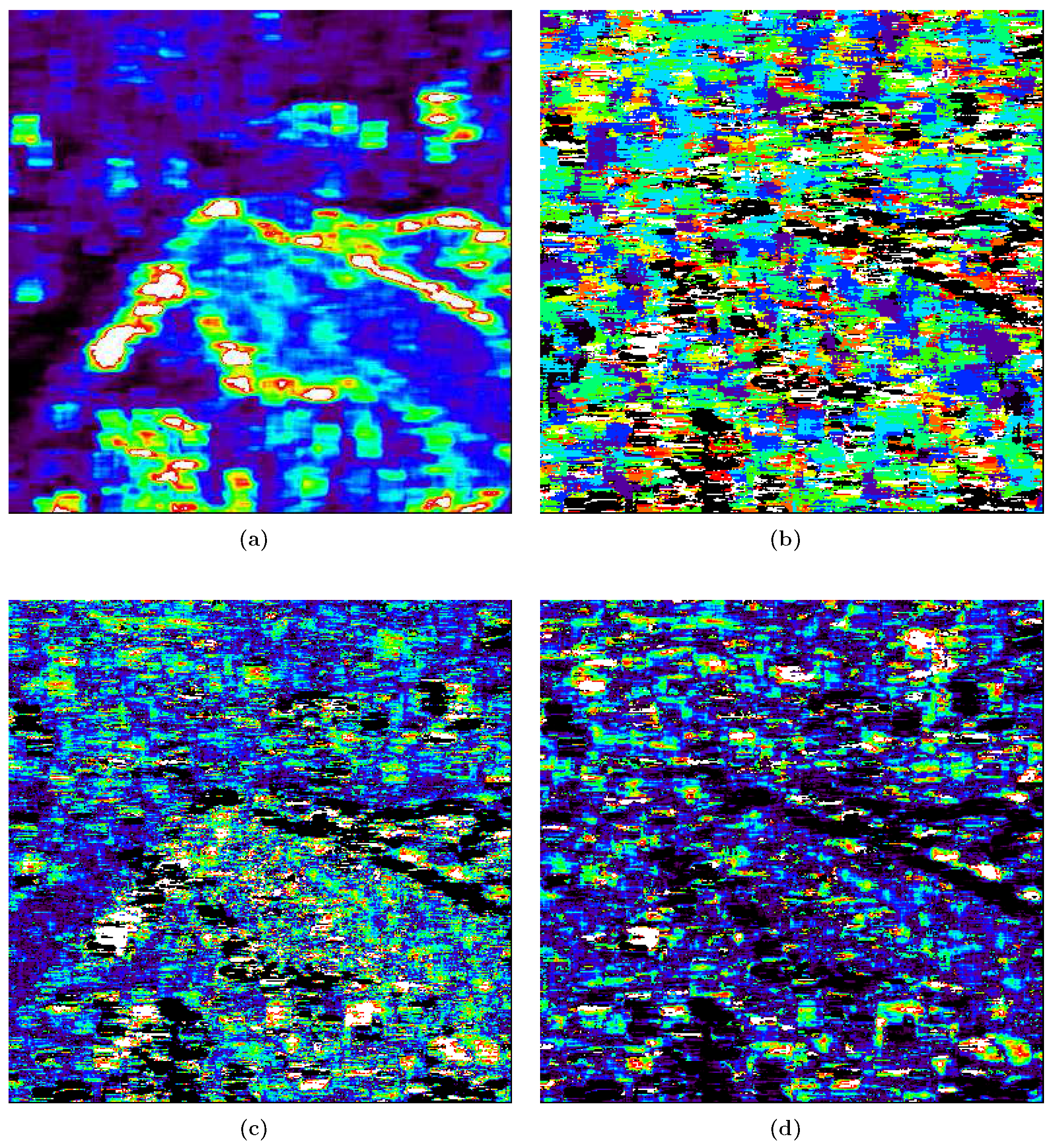
From the RADARSAT data set (
Figure 3a), parameter maps were derived for vario parameters
,
,
and
, each for directions 0 deg and 90 deg and for window sizes of 20 and 40 pixels with an offset of 1 (see
Figure 5,
Figure 6,
Figure 7 and
Figure 8). The offset value is the same in directions of rows and columns (offset 1 means, the first window contains a submatrix of rows 1–40 and columns 1–40, the second window rows 1–40 and columns 2–41, etc.) and determines the size of the output image (here: 400 − 40 + 1 = 361, 400 − 20 + 1 = 381, derived from Equation (1), since both
and
need to lie inside the region
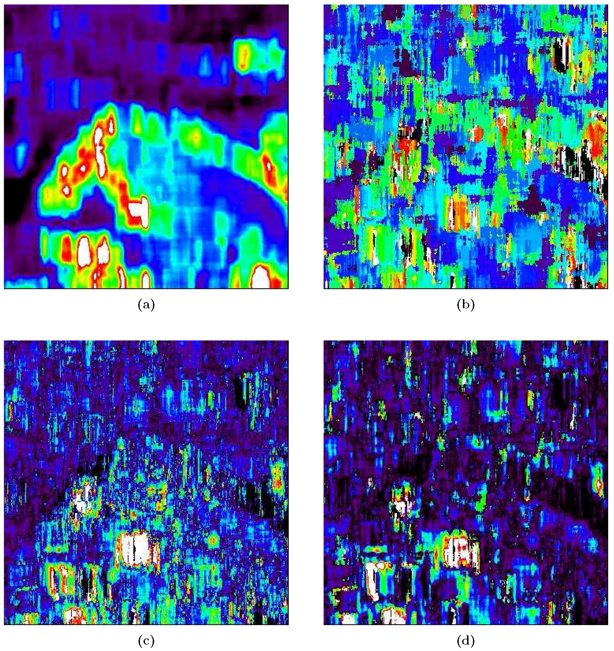
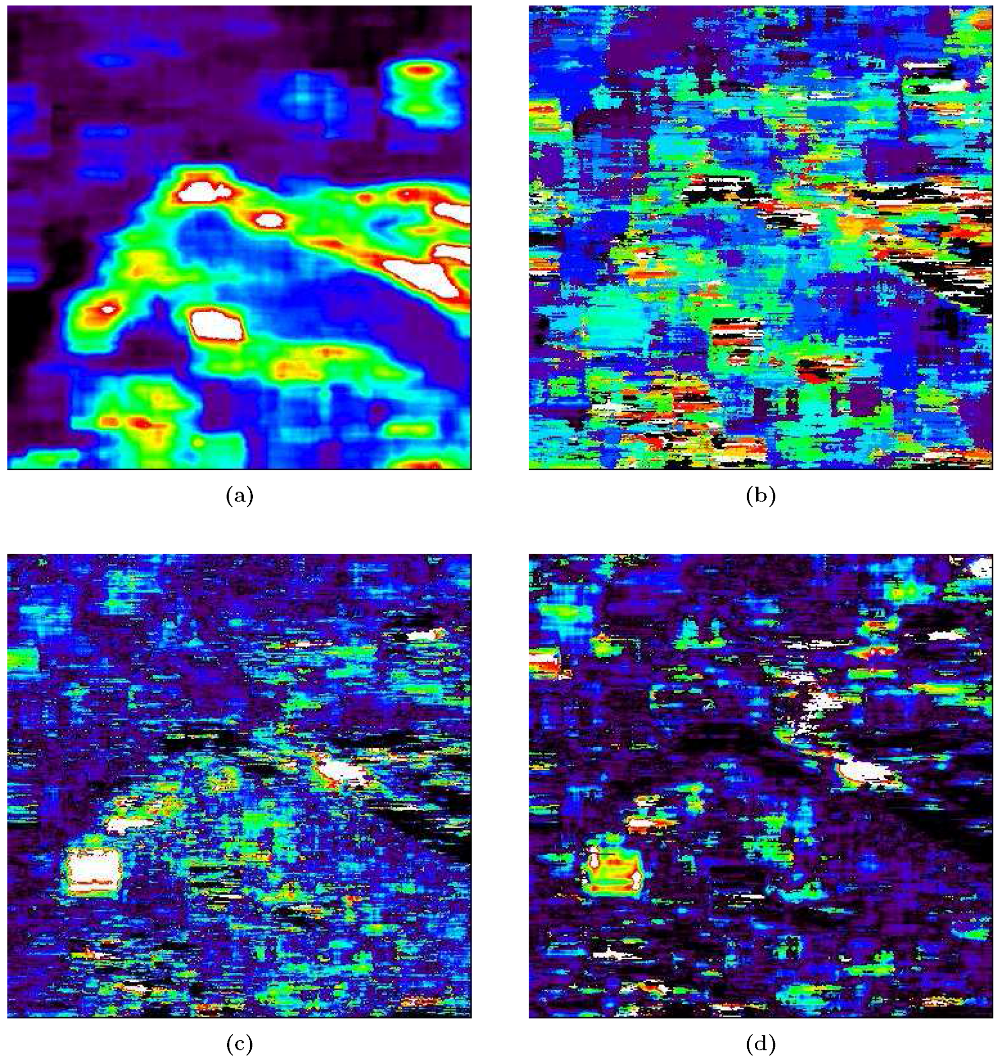
, which in our study corresponds to the SAR image; i.e., the output image has the same size as the input image minus a margin, and the same resolution as the input image). Parameter maps calculated with window size 40 have a larger smoothing effect than those resultant from window size 20. Given the relatively large size of the SAR pixels (75 m) relative to sea-ice features, a window size of 20 appears preferable. In the following sections, parameter maps are compared to the target classification image (
Figure 3c) for validation of results.
6.1. Parameter Maps for Pond
For the same material, the
parameter indicates the overall roughness of the surface at the observed scale. Areas with lowest
parameter values are mapped in the Chukchi Sea close to the spit (which in fact is an area of very smooth ice) and in Elson Lagoon (which comprises several types of smooth ice). In Elson Lagoon two distinct subprovinces can be identified in the RADARSAT SAR data (cf.
Figure 3c) , whereas five subprovinces have been identified in PSR data and snow-depth field data (
Figure 3d). Subarea 2 contains significant changes in the SAR data reflectance value, which may be attributed to small-scale surface structures or to local spatial changes between wet and dry areas, causing strong reflection differences. The
parameter indicates changes in surface characteristics, measured and summarized as variability in reflectance properties. On this basis, the
parameter facilitates a segmentation of the SAR image into provinces that match those in the target image (
Figure 3c), and additionally, more subareas can be identified in the northern third of the image, which stand out optically in the SAR image. In case of the
parameter map, both window sizes are equally well suited, as no distance measures are involved.
The parameter may be considered as a first indicator of the degree of morphogenetic processing that an area of sea ice has experienced, with a larger value indicating more steps of morphogenesis. Material changes may be due to diagenesis of snow and ice. Reflectance properties also depend on the geometry of the surface, such as exposure of parts of the surface in different directions (slope aspect).
6.2. Parameter Maps for Mindist
Considering that several types of processes are found to contribute to changes in the SAR value, the amount of variability (as in
) does not allow a unique interpretation. Independently of the source of variability (elevation, material, aspect, etc.), the size (or correlation length) of surface features is an additional parameter that is suitable for characterization of a sea-ice type. The size of such features is captured in the
parameter (see
Figure 5b,
Figure 6b,
Figure 7b and
Figure 8b). Comparison of the
parameter maps with the target image in
Figure 3c indicates that
indeed matches the sizes of surface features in the image, with a lack of accuracy due to the lack of resolution in the SAR data.
6.3. Anisotropies
Anisotropies can be mapped and quantified comparing vario-parameter maps created for directions 0 deg (east–west) and 90 deg (north–south). Comparing
Figure 5 with
Figure 6, and
Figure 7 with
Figure 8 for matching panels, it is obvious that for each parameter the maps calculated for 90 deg vario function differ from those for 0 deg variograms. This observation implies that the sea ice is anisotropic in each province. The 0 deg maps and the 90 deg maps yield approximately the same segmentation of the study area into provinces. The parameter most suited for quantification of anisotropy is
. In general, in situations of geometric anisotropies characteristic distances are best derived from profiles normal to the strike of the dominant features in the area, as spatial variability is highest in this direction and characteristic distances are shortest. In the eastern part of Elson Lagoon, anisotropic characteristics are least distinct compared to other areas in the study area,
values are about the same for both directions (see e.g.,
Figure 5b and
Figure 6b), hence the ice may be considered close to isotropic. In the Beaufort Sea, the strike of features appears to dominantly be close to E-W, which is concluded from the fact that the
map for direction E-W (
Figure 5b) has more connected areas than the
map for direction N-S (
Figure 6b), the latter one has a striped appearance which results from quickly changing
values among neighboring windows. For the Chukchi Sea areas, the same comparison yields a different picture, and there are even differences between the northern and the southern Chukchi Sea parts in the image. Hence the main direction of orientation of surface features is variable in the Chukchi Sea; in the northern area near Point Barrow it appears to be closer to 45 deg than to 90 deg, this is the area of floe striata that shear off the tip of Pt Barrow and extend north-eastwards, then eastwards.
In a mesoscale analysis of LANDSAT MSS data, Hibler III et al. [
71] noticed that the pack ice in the Beaufort Sea moves as a gyre with clockwise rotation, but that maximal shear, which induces counterclockwise rotation, occurs in a 50 km wide zone between the shorefast ice and the moving pack ice. Hence the orientation changes counterclockwise in the area of Point Barrow, which matches our results on anisotropy, notably based on analysis of a single image in two directions.
These observations indicate differences in wind and current directions in the Beaufort Sea and the Chukchi Sea that likely have lead to the formation of large ridges as observed in the Beaufort Sea and of ridged ad rubbled areas. To identify the direction of main orientation accurately, one needs to calculate 8 directional variograms or determine parameter
, the direction of the closest minimum (see Herzfeld andHigginson [
49]). As a methodological conclusion, we note that parameter
derived from vario functions of different directions may be employed to identify directions of ice drift and of compression or overthrusting of sea ice.
6.4. Parameter Combinations
The significance parameters and indicate the importance or significance of those spatial features whose sizes are quantified by . A combination of , with the value reveals structural properties of the surface, in the following sense: A large value combined with a large value indicates a surface with large and morphologically outstanding features. A small value with a large value means that the surface has long-waved but shallow structures. If is small, but is large, then the surface has short-length, but significant features, and a high roughness at small scale. Now assume that a feature A has the same amplitude as feature B, but a larger value, then , but . Parameter is termed relative significance parameter, because a large parameter stands for features with a large significance relative to their size. A large parameter (slope parameter) indicates features that are absolutely large and also significant.
With the help of parameter combinations, we are now able to discriminate different characteristics of Beaufort Sea, Elson Lagoon and Chukchi Sea ice provinces. Beaufort Sea and Chukchi Sea have similar parameter values, and different from Elson Lagoon’s. One can also identify subprovinces in the Beaufort and Chukchi seas simply on the parameter maps. Parameter serves to differentiate between the Elson Lagoon ice and the sea ice in open waters in the Chukchi and Beaufort seas, whereas maps seem to be to locally variable for visual interpretation; however, an automated combination of parameters is expected to lead to a segmentation (see Applications (A.3) and (A.4)).
6.5. Interim Conclusions
Vario-parameter maps allow to automatically identify several spatial characteristics of sea ice types from RADARSAT data, including size of dominant features, prominence (significance) of dominant features absolutely and relative to their size, and maximum spatial variability of reflectance properties. The combination of these properties may be useful for a characterization of sea-ice types. In the example, the parameter maps, viewed together, indicate an Elson-Lagoon type with short-based but at small scale significant features, with likely a mix of wet and dry surfaces responsible for the high value; rougher surface in Beaufort Sea with long-waved features of similar significance to those in Elson, with two subprovinces, a smoother province and a rougher province; and sea-ice types in the Chukchi Sea with lower overall variability and slightly lower significance than in Beaufort. The sea ice in each province is found to be anisotropic, however, ice in eastern Elson Lagoon is closest to isotropic; ice in the Beaufort Sea is dominated by features that strike approximately north-south, while anisotropies in the Chukchi Sea vary in direction.
The interpretation in this application depends on comparative visual interpretation of several parameter maps, which in itself may already be considered classification maps or thematic maps. Because of the complexity of information contained in each individual parameter map, an automated classification based on parameter maps as inputs may be more user-friendly; this approach is followed in the next applications.
7. Application (A.2): Geostatistical Characterization of Sea Ice from ERS-2 SAR Data (December 2005)
Parameter maps were calculated for the all of the following combinations of directions, resolutions and step sizes: {dir0, dir90}{w20, w40}{s1, s2} and a large number of parameters. Parameter maps resulting from a step offset of 1 pixel are close in appearance to those with stepsize = 2. Since the features of interest are already poorly resolved in SAR data, a step size of 1 is most useful.
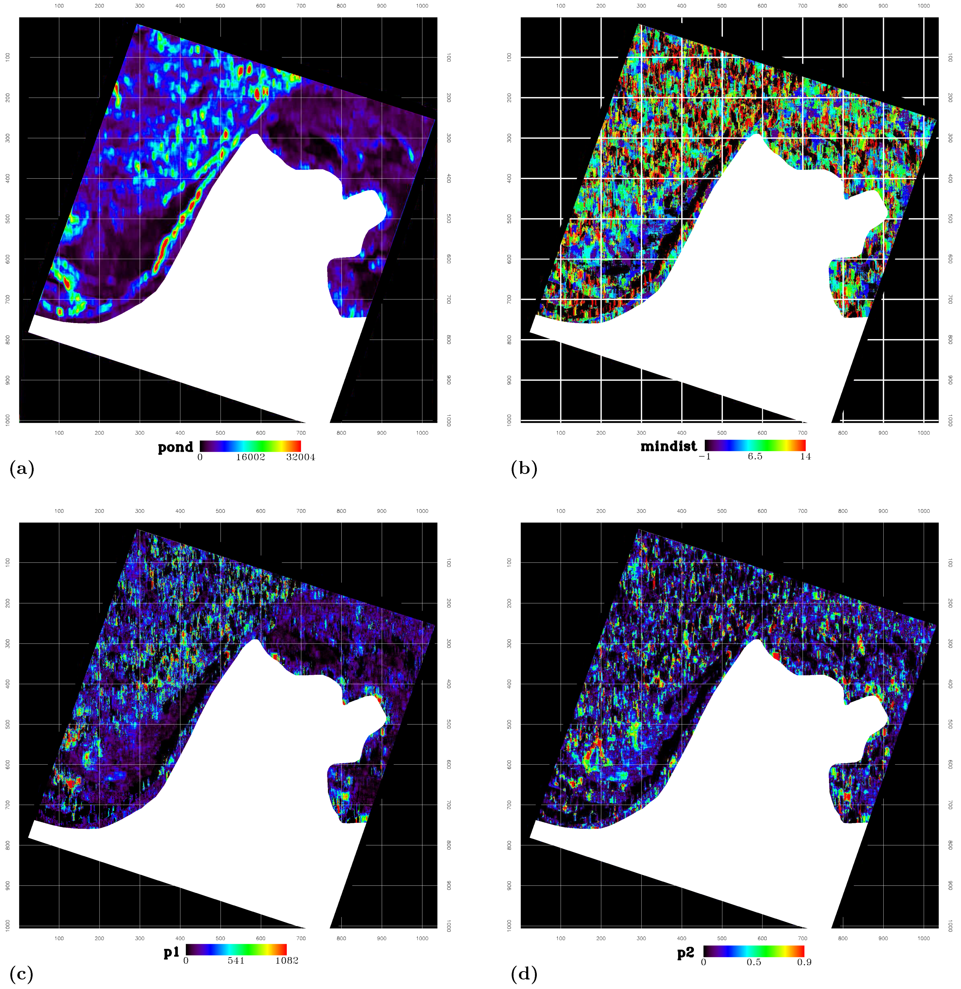
Figure 9 shows the resultant parameter maps for
,
,
and
, for direction 0 only and step size 2 and w = 20. However, dir90-parameter maps will also be used in the next steps of analysis. In the next sections, we interpret and discuss results of parameter maps for
.
7.1. Parameter Maps for Pond
The value of the
parameter relates to overall roughness length. The areas with lowest roughness are in parts of Elson Lagoon and close to the shore in the Chukchi Sea and in the Beaufort Sea; this matches the location of smooth ice derived in analyses of field and PSR data from March 2003 (Herzfeld et al. [
31]) and therefore indicates that the areas of smooth ice remain approximately the same throughout the winters. Elson Lagoon segments 1 and 5 (as identified in
Figure 3d and Table 1 in Herzfeld et al. [
31]) have lowest
values throughout the study area for snow-depth field data, in the SAR data, segments 1, and 2 have lowest values, followed by segment 5. Between those lies segment 4, which has
from field data, which corresponds to a low-intermediate value of pond in the ERS-SAR parameter map (blue color). We find a general agreement, however, the field and aerial surveys convey a lot more detailed information.
The western shoreline and the spit stand out visually, with red-green colors (
Figure 9). The Chukchi area close to shore is mapped with lower values, matching the low pond value (pond = 2.4) in snow-depth data and the brightest blue in the PSR data, both characteristic of the smooth ice that is protected by the stamukhi zone. (Note that PSR data are presented as a color composite to facilitate visual comparison.) Further seaward, the pond map derived from ERS-2 data shows higher values in good agreement with the brown-colored area in the PSR map, both indicative of higher roughness associated with the stamukhi zone’s ridging. In summary, the
parameter can be used to map sea-ice provinces by overall roughness based on SAR data, matching field observations modulo the expected loss of detail.
Results from the field data analysis indicated that a combination of several parameters is better suited to characterize sea-ice complexity and spatial roughness than a single parameter (Herzfeld et al. [
31]). A similar observation holds here: more parameters may be needed for a classification based on SAR data, which leads to the next step of combining parameters maps (see, Applications (A.3) and (A.4)). First, this requires to determine useful additional parameters.
7.2. Parameter Maps for Mindist
The next interesting parameter is the size of features, which may be quantified by the
parameter (see
Figure 9b). Here we use the color-enhanced ERS-2 SAR image (
Figure 4b) as a validation basis (see also
Figure 3c, as some provinces remain throughout several seasons or reform). In the Chukchi sea, the color-enhanced SAR image shows an area of floes of various sizes, with a trend to increase in size with distance from the coast. The size variability is reflected in the multi-coloring of the
map in the same area, whereas the smooth area has a dominance of short distances (light-blue to blue) or no features of discernible correlation length (black). The smooth area coincides with the area that appears white in the original SAR image. Notably, this smooth area has lower mindist values than much of Elson Lagoon, which also matches the observation that Elson Lagoon ice falls into several different subclasses, which are all more complex than the smooth area in the Chukchi Sea. In terms of a characterization, we note that
values differ more than
values, comparing Elson Lagoon and the smooth area in the Chukchi Sea. The
parameter appears useful to calculate sizes, but the distribution across a large range of values (colors) suggests that a higher-order parameter is needed or a classification that summarizes parameter values further.
Material sheared off in pieces at the tip of Point Barrow creates striated floes off the point, as noted in the visual interpretation of the SAR data set. The area of striated floes has lower roughness and contains fragments of smaller sizes than the lower end of the size range of ice floes in the Chukchi Sea.
We note further that the size classification with works independently of the reflectance properties of the surface of individual ice pieces, thereby adding another component of information in addition to backscatter and the parameter. Several components of information may be combined into a feature vector, an approach to be followed in application Sections A.3 and A.4.
7.3. Parameter Maps for p1 and p2
The significance parameters and are designed to distinguish between surface types of absolutely large roughness and surface types dominated by features that are absolutely small, but cause significant roughness at a small scale. Large features with absolutely large significance will have a relatively large value and a relatively large value. Small features with relatively large significance will have a relatively large value, but a relatively small value. (Note that can assume any value, whereas is always absolutely less or equal to 1). This difference in concept is well exemplified in our study area.
In the Chukchi NW corner of the study area, results of
and
calculations are similar, since large-scales floes dominate.
-values in area (2) (as identified in the visual interpretation of the color-enhanced SAR data,
Figure 4b and
Section 3.2) are overall higher than elsewhere in the study area. However, in the boundary of area (3) Chukchi South, in areas in Elson Lagoon and in the Beaufort sea,
reaches values of 0.9, whereas
values are in the lower range. High
values occur since small pieces with high variability are frequent (water-flow boundaries are crossed more often, which leads to high
values, while the ice is absolutely fairly smooth, as implied by the lower
values in these areas). The different meaning of parameters
and
is most obvious in the overall smooth area in the Chukchi Sea and in the Elson/Beaufort region. Narrow but strongly contrasting lines associated with the striated floes in the Beaufort Sea receive a low
value but a high
value. In entirely smooth areas lacking even small-scale roughness features, both the parameter
-map and the
-map have low values (e.g., in the southern part of the Chukchi Sea in the study area). Therefore, a
-vector may be utilized for detection of areas with small-scale openings, such as arrays of narrow leads, or other contrasting lineaments.
7.4. Anisotropy
The structures here are of an anisotropic nature, reflected in differences between the directional parameter maps. The latter observations warrant an inclusion of two sets of directional parameter maps in the feature vectors (see (A.3) and (A.4)).
7.5. Interim Conclusions
The individual parameter maps are useful to map roughness properties, specifically:
overall roughness is mapped by ,
average size or spacing of dominant features, similar to correlation length, is calculated by ,
is most useful to detect anisotropies,
absolute significance of roughness structures is quantified by , and
scale-independent significance of roughness features relative to their size is identified by .
Parameters , and map spatial properties independent of the reflectance of the surface.
A combination of p1 and p2 may be used to detect narrow openings, leads and swarms of openings.
A combination of parameters , , and promises to be a good basis for a segmentation.
In some cases, a single parameter map is sufficient to distinguish between sea-ice provinces, and hence a parameter map may be considered a special case of a classification map, enabling a segmentation into larger provinces. In other cases, a combination of parameters , , and may be required for a classification and segmentation.
8. Multivariate Statistical Classification Based on Feature Vectors of Geostatistical Parameter Maps—Method
Approaches to an automated classification based on several parameters require building a feature vector and then applying an association or class discrimination algorithm. In the sequel, we utilize the following approaches:
- (a)
an unsupervised classification, using a statistical technique (k-means clustering)
- (b)
a supervised classification, using a maximum likelihood classifier and demonstrate the main differences between a supervised and an unsupervised classification.
The general form of the feature vector is
where
is a geostatistical vario parameter, calculated for a window centered on location
x. Hence the feature vector is a functional moving throughout the area. In our application cases, the feature vector is composed of parameters
,
,
,
, either in 4 components for a single direction or in 8 components for two directions:
or
where the indeces (000) and (090) indicate calculation in directions 0
(east-west) 90
(north-south) respectively.
In case studies (A.3) and (A.4), an artificial image of four (or eight) “bands” is created in ENVI (Research Systems Incorporated (RSI) Software, v. 4.2, IDL v. 6.2, 2005, now ENVI classic), where each of the parameter maps , , and constitute a “band" of an artificial multispectral image. This trick allows one to apply multivariate statistical methods, operating in the feature vector, for each location in the image area.
9. Application (A.3): Unsupervised Statistical Classification Based on Feature Vectors of Parameter Maps
Unsupervised classification determines classes following an automated algorithm, without previous knowledge of the classes. Unsupervised classification is easy to perform by the user, however, the user is then left with the task of interpreting the resultant classes, which may or may not be possible. Here the k-means clustering algorithm was applied, which uses a cluster analysis approach that requires the user to select the number of clusters (classes) to partition a multi-dimensional data set, arbitrarily locates the given number of cluster centers, and then iteratively repositions the centers by aiming to minimize the within-cluster sum of squares (sum of squared distances between the center and a point, for all points in the cluster; Swiniarski et al. [
72]). The k-means unsupervised classification was run in ENVI classic (RSI 2005).
In the first case study, a classification is based on 4 input maps, the parameter maps for
,
,
and
, calculated in direction 000 with window size 20 pixels (parallel to the right-hand axis in the original orientation of the SAR data set), using a feature vector as in Equation (
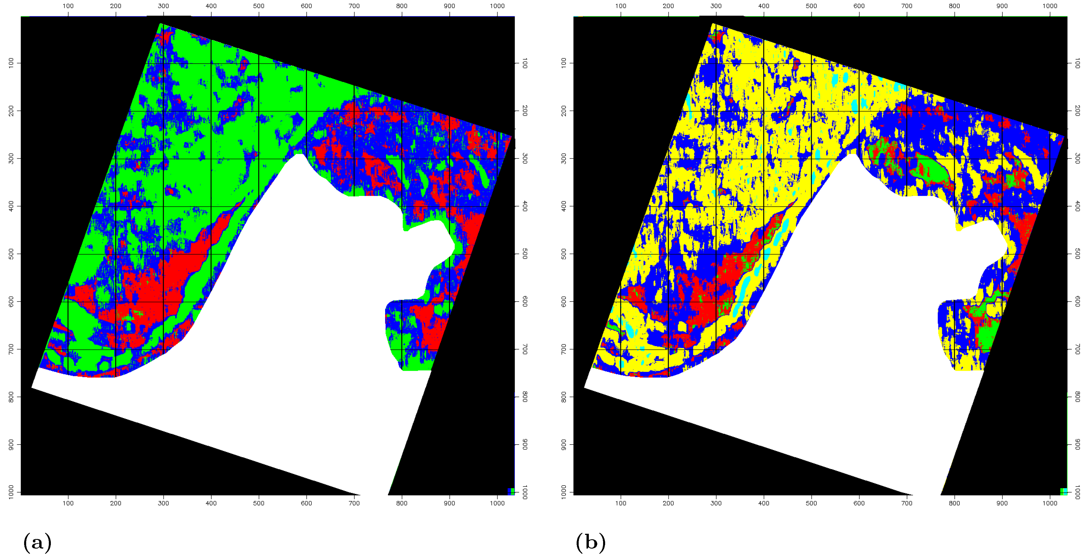
featv.1). The k-means clustering routine, run with 10 classes and a threshold of 5% pixel value change to stop iteration, yields the classification map in
Figure 10a. The routine stopped after 3 iterations. The unsupervised classification is somewhat successful in identifying the correct areas (1, 2, 3, 4 in the visual classification,
Section 3), however, the individual parameter maps are more clear and easier to interpret than the classification map. The fact that the land area is also classified may be distracting, but this is not essential. The lake ice does have spatial properties similar to the sea ice in the smoother regions. A problem lies in the fact that the unsupervised k-means routine aims to match centers in clusters, but the parameter variables are scaled differently and the classes have non-linearly different ranges.
To incorporate anisotropies in the classification, the eight-parameter feature vector given in Equation (featv.2), using directional vario functions in two orthogonal directions (0 (east–west) and 90 (north–south)). In this run, the classification routine stopped after 1 iteration, with the same 5% threshold as in the first experiment. The result is better than from the 4-component vector, noting that the 3 areas Chukchi-south, Chukchi-N, and Elson have less fuzzy delimiters. In summary, results of the unsupervised classification are not satisfactory.
10. Application (A.4): Supervised Statistical Classification Based on Feature Vectors of Parameter Maps
In a supervised classification, the algorithm for association is trained based on areas of known classes. Several areas of known sea-ice type were selected manually as “regions of interest”, following the manual segmentation given in
Figure 4. We used 3–10 areas in a number of example runs, based on a 4-component feature vector as in Equation (featv.1), for maps calculated with window size 20 and step size 1. Selected resultant maps are seen in
Figure 11.
Figure 11a shows the result of a simple supervised classification based on only 3 training areas (smooth ice, ice of intermediate roughness and scale in Elson Lagoon, and rough ice of large spatial scale and large p1 and p2-parameter values, as found in the Chukchi NW corner). The classification is successful at separating these classes, but several class types are summarized into a single class.
In the second example (see
Figure 11b), 5 training types of 1 and 2 samples each were used. This classification succeeded in mapping (1, red) the Chukchi smooth zone differently from the (2, green) Elson smooth zone, (3, blue) rougher (higher
) and spatially more varied ice of smaller characteristic sizes in Elson Lagoon with low
and high
values; this class then included the Beaufort sheared striated floes and Chukchi stamukhi zone, (4, yellow) areas of large floes with high significance in the NW Chukchi corner (seems to put less striking features in Elson in the same class) and (5, cyan) areas of highest roughness (only small regions were associated to this class, including the shore because of the land-ice contrast along the shore and spit).
Notably, the classification algorithm is able to associate ice in a bay on the east side of the map (where it was not trained), similar to Elson Laggon (see
Figure 2). The ice in the eastern lagoon appears to be classified correctly, similary to Elson Lagoon. Comparison of the results obtained in this section with the results of the unsupervised classification in
Section 9 demonstrates (1) that the supervised classification is clearly superior, as expected; and (2) that the combination of parameters and classification algorithm determines the quality of the results. The examples in this section yield better results, while fewer parameters (feature-vector components) are employed. Application of the same classification to the four parameters derived for the orthogonal direction gave similar results, which indicates that in this example the anisotropies in the ice-surface morphology are not needed to separate the classes. This is not always the case, as the classification of seafloor morphology in Herzfeld and Higginson [
49] shows.
11. Discussion: Comparison of Different Approaches to Sea-Ice Characterization and Classification
The problem of sea-ice classification has evolved into an area of active ongoing research. Early research on sea-ice classification was motivated by understanding sea-ice movement and mapping of a small number of ice types. Researchers in regions bordering the Arctic oceans, including Canada, Finland, Norway and the United States of America have been interested in sea-ice forecasting and recently derived classification methods for SAR data analysis. Along with this, interest shifted to deriving a larger number of properties from imagery. A relatively new application is model-data comparison and evaluation of physical sea-ice models. In this section we summarize some of the history of the problem to lead to a comparison of recent approaches and goals in applications of this topic.
11.1. Analysis of SAR Data for Sea-Ice Classification
The potential for using radar to detect sea ice was recognized in the 1970s, although at that time technology permitted only discrimination between sea ice and ocean surfaces (Parashar [
73]). Later laboratory and field studies (Barber et al. [
74], Grenfell [
75]) showed that the backscatter of sea ice undergoes a profound evolution as the ice grows and changes. However, because multiple sea ice states can have the same backscatter values (Grenfell et al. [
76]), backscatter at a single pixel is insufficient to distinguish between ice categories. Steffen and Heinrichs [
77], using Landsat data as “truth”, found that first-year and old ice in winter can be separated using single-point C-band SAR backscatter but that performance is much worse in other seasons and for the thinner ice types. The performance of a single-pixel classifier can be improved by cluster analysis (Kwok et al. [
78]), but most work in recent years has been based on incorporating the spatial information present in SAR images. Most of these approaches calculate measures of spatial variability in a window or neighborhood around each pixel in a SAR image, and then employ supervised or unsupervised classification of those measures to segment the image.
Texture feature vectors are the most commonly used, most often those derived from the gray level co-occurrence matrix (GLCM), which represents the occurrence of a possible pair of gray levels measured at two pixels as a function of the displacement vector between the two pixels (Shokr [
79], Soh and Tsatsoulis [
80]). Shokr [
79] found that of the many texture measures available, the inverse difference moment and entropy produced the best results. Gill [
81] also found an entropy measure to be effective in classifying SAR images of sea ice. Bodanov et al. [
82] used texture measures from Markov Random Fields (MRFs) and probabilities derived from the GLCM to classify sea ice, with segmentation by Linear Discriminant Analysis (LDA) and a neural network, and found that the neural network had better results in classification open water and nilas while the LDA algorithm performed better for classification of deformed first year ice. Yu and Clausi [
83] used a Filament Preserving Model with MRFs and found that their new model was better able to distinguish linear features such as ridges and leads. Deng and Clausi [
84] used a Bayesian probability model with Markov Random Fields in an unsupervised classification and found better performance distinguishing first-year smooth ice, first-year rough ice, and multiyear ice. Karvonen [
85] used pulse-coupled neural networks for classifying SAR images over the Baltic Sea and an automated training technique based on decomposing the total pixel value distribution into a mixture of class distributions. Their results were promising, but fast ice was classified to multiple classes and frozen brash ice could not be distinguished from highly deformed ice areas. Karvonen and Kaarna [
86] used non-negative factorization methods to classify sea ice and found that these algorithms can produce useful features for classifying SAR data based on texture. However, geophysical interpretation of their results proved to be difficult.
The major limitations of early classifications are related to information visible in the images that is not incorporated in the classification algorithm. None of these studies listed above claim to be able to reproduce ice classification with the quality of a trained ice analyst. Maillard et al. [
87], using the Markov Random Field and texture inputs, and with ice maps produced by the Canadian Ice Service, found performance between 71% and 89% compared to a trained ice analyst. They attribute the limitations in performance to sub-scale information on floe size and shape available to human analysts, but not incorporated into the classification system. It is worthwhile to point out that the US National Ice Center and other operational ice monitoring agencies still use ice analysts to visually interpret SAR imagery (Bertoia et al. [
88]). Many of those problems are attributable primarily to features that arise through dynamic and morphogenetic processes in the ice.
11.2. From Simple to Complex Variables
The two variables that are most commonly analyzed in the literature are velocity and thickness. Sea-ice thickness is not typically derived from imagery, but from satellite or airborne altimeter data, as summarized in the introduction. Techniques for the determination of sea-ice motion from satellite images at large scales are described or referenced in Holt et al. [
89], most of these utilize vector-based algorithms that are applied to differences derived from two or more images. A method for derivation of high-resolution velocity fields from SAR data is discussed by Karvonen et al. [
32].
An approach for identification of sea-ice types, namely multi-year ice, first-year ice and thin ice, from SAR data using a radar-lookup table, a minimum-distance classifier or a maximum-likelihood classifier is described in Kwok et al. [
78]. In the lookup-table method, the backscatter value of each pixel is associated directly to one of the three classes, whereas in the other two methods, the variance in a cluster of pixels also plays a role. An interesting statistical concept for sea-ice classification is suggested by Collins [
90], based on a “theory of belief”, which is a generalization of Bayesian statistics, and on neural networks, but unfortunately no applications are presented. In summary, none of these methods facilitate distinction of more than basic characteristics in very few classes.
Sea-ice thickness distribution functions have been successfully applied to summarize ice properties over large areas (Rothrock et al. [
3,
91], Pritchard et al. [
92]). A community need identified in Wang et al. [
93] is that to run larger-scale models, a parameterization of small-scale models is needed. Significant progress in small-scale (less than 10 km) ice-ocean modeling was made during the RADARSAT Geophysical Processor System (RGPS) project (Wang et al. [
93], Kwok [
94], Coon et al. [
95]). A major obstacle in the development of such models is the verification through data analysis (Wang et al. [
93]).
Work on small-scale kinematics and dynamics of sea ice (Pritchard et al. [
92], Coon et al. [
95], Hibler III [
96]) is based on the principles of structural mechanics and rheology. Examples of structural mechanics models lead for instance to patterns of deformation in sea ice, such as shear, 2-dimensional or 1-dimensional extension or compression, which result in typical patterns (e.g., Wang et al. [
93]). Wang et al. [
93] in their summary of status quo versus needed tasks state that high-resolution models can reproduce oceanic eddies and fractures zones qualitatively, but not validate those models from data.
The topic of linking properties that can be derived from imagery with physical properties and processes of the sea ice has been limited by the simplicity of statistical approaches applied and to the lack of recognition of the scale problem. Karvonen’s work [
32] provides a milestone in state-of-the-art statistical techniques in sea-ice classification, but applications are limited to the Baltic sea, which has a seasonal ice cover. Karvonen et al. [
32] note that understanding physical processes is an open problem.
11.3. Recent Developments
Most recent methods continue to use multivariate statistics at the pixel value, for example Ochilov and Clausi [
97], Wang et al. [
98], Dabboor and Geldsetzer [
99]. The differences between those methods and the geostatistical characterization and classification method are that (1) the geostatistical approach derives vario function values from sub-images of an intermediate size that is large enough to capture characteristic repeating morphological features; and (2) the characterization or classification is then based on parameters that are calculated from the vario functions in order to summarize spatial properties, rather than on the vario function values themselves. Dabboor and Geldsetzer [
99] utilize 23 statistical parameters. In Herzfeld et al. [
61,
100], Herzfeld [
55] we have introduced a large number of parameters to capture different levels of feature complexity that occurs at several different scales, however a too large number of individual parameters then may introduce unnecessary numerical complexity at the next level, the actual classification step. Therefore in Herzfeld et al. [
31], Herzfeld [
55] we introduced summarizing classes of hyperparameters as a means to provide a hierarchical structure to the set of spatial parameters that may be useful in a given application.
In the geostatistical classification method described here, the classification builds on feature vectors of parameter values and the result yields a segmentation of the study area into regions of different sea-ice types (as illustrated in
Figure 10 and
Figure 11. In this respect Ochilov and Clausi [
97] present a different approach that bases the segmentation on gradients in the original multivariate statistical parameters, using an edge-detection method. Only three classes result this way from a single image (gray-white, gray and new ice). Owing to the analysis of larger window sizes and parameters aimed at detecting morphological complexity, the geostatistical classification method allows to distinguish several sea-ice types that describe the deformation state and indicates levels of kinematics experienced inside a sea-ice province. The conceptual difference is that the geostatistical method is in part motivated by concepts of structural geology, whereas most other methods appear to be motivated by simple characteristics of sea ice (spectral properties , new vs old ice; e.g., Kwok et al. [
78]). As a consequence, a structurally based approach facilitates model-data comparisons aimed at identification of the old, deformed ice (whose decline in the Arctic ice cover has been identified as a critical indicator of Arctic ice retreat altogether, see Herzfeld et al. [
24]. A notable exception that includes the concept of deformation is the work of Zakhvatkina et al. [
101] which uses the gray-level co-occurrence matrix for windows of 2, 4, 8, 16 or 32 pixels in an ENVISAT SAR image, then employs a number of statistical parameters including correlation, inertia, cluster prominence, energy, homogeneity, entropy and 3rd and 4th order statistics moments and finally a neural network to separate (1) deformed first-year ice; (2) level first-year ice; (3) multi-year ice and (4) open nilas. The neural net approach works well in the end, but the training process is complicated and specific to the problem at hand. A combination of the geostatistical classification method and a neural network (a feed-forward multi-layer perceptron with back-propagation of errors) is described as the connectionist-geostatistical ice-surface classification method in Herzfeld and Zahner [
45], Herzfeld et al. [
102] and applied to surge crevasse types for the Bering Bagley Glacier System, Alaska. Karvonen Karvonen [
103] uses a multi-layer perceptron as part of an operational algorithm for estimation of sea-ice concentration from dual-polarized RADARSAT-2 ScanSAR data and applies this to observations of the Baltic Sea ice.
A paper that contributes to analysis of a component of ice kinematics without using a classification is the following: Motivated by the observation of a tail in the sea-ice thickness distribution of ice along the Arctic coasts of Greenland and the Canadian Arctic Archipelago, Kwok [
104] introduces a normalized ice convergence index to examine the variability and extremes in convergence of the Arctic sea ice from 1992–2014 passive microwave data. The study indicates a potential impact of ice dynamics on observed variability of summer ice extent in 2013 and 2014.
In summary, the research of sea-ice classification has moved from classification of simple properties (such as color, new ice versus older ice) to identification of complex property sets that may allow association with physical properties and processes that describe physical characteristics dynamics and deformation states of sea ice and, as such, facilitate comparison of information that can be derived from SAR imagery (and other data) with information can can be derived from numerical sea-ice models. Further research is needed towards this goal.
12. Conclusions
The approach to SAR-data classification for sea ice derived and applied here is a two-tiered one, combining (1) geostatistical characterization/classification and (2) multivariate statistical classification based on step (1). The method is applied and evaluated here for shore-fast sea ice and near-shore pack ice in the neighborhood of Point Barrow, Alaska, which includes Elson Lagoon and parts of the Chukchi Sea and the Beaufort Sea. SAR data from two satellites, the Canadian RADARSAT-1 and the European ERS-2, are analyzed.
Salient ideas of the approach include the spatial surface roughness concept, which can be used to characterize and discriminate sea-ice properties and provinces (where the term “province” is used as in structural geology) and the realization that spatial variability measures, such as variograms and their discrete-mathematical counterparts, vario functions, can be employed to analyze spatial surface roughness. With the geostatistical classification parameters, or vario parameters, the paper introduces new parameters to SAR classification, and to texture analysis/feature analysis/image analysis in general. In an abstract sense, the parameters quantify overall roughness or reflectance variability (caused by geometric features or wetness differences or exposure to the incoming signal), spacing and significance of scale-dependent and scale-independent structures. The parameters relate directly to sea-ice morphogenetic properties, including smooth ice areas, areas of small-scale rubbled ice, spacing of leads and swarms of openings, sizes and structures of older, more complex and younger ice floes. Individual parameter maps, such as the map, may serve to distinguish several provinces, simply through spatial variability in reflectance. For example, the parameter separates subprovinces in Elson Lagoon, smooth and very smooth ice areas in the Chukchi Sea and in the lagoon, stamukhi zone ice and areas of older ice in the Chukchi and Beaufort seas.
A multivariate statistical classification based on several parameter maps is enabled by means of the feature vector concept, where the components of the feature vector are the parameter operators. Comparing an unsupervised classification based on k-means clustering and a supervised classification using a maximum-likelihood classifier, the supervised classification yields good results, whereas the unsupervised classification works less satisfactorily. The combination of supervised classification with geostatistical classification yields the best results for segmentation of the study area into sea-ice provinces, automatically identifying two provinces in Elson Lagoon, an area of striated floes northeast and east of Point Barrow, the Chukchi smooth ice area and the stamukhi zone, areas of smoother, young ice and older ice in the Chukchi sea, and other ice provinces as noted on the target map. Field data were available for validation of some of the results. As a conceptual difference, we note that the characterization/classification through vario parameter maps yields ice types, or ice classes, whereas the combined multivariate classification based on vario parameter maps yields an automated segmentation, i.e., an automated thematic mapping of sea-ice provinces. The supervised classification requires a priori knowledge of some sea-ice prototype areas, whereas the geostatistical characterization is fully automatic and operates without a-priory knowledge.
The strength of the geostatistical characterization and classification approach stems from the facts that (1) the vario function both summarizes and enhances spatial and spectral characteristics of the ice-surface at a spatial scale that can be adapted to the problem and data set at hand, by setting the window size and unit lag of the vario function; and (2) the vario parameters then serve to extract characteristic values from the vario functions. The classification is then based on the parameters (composed into a feature vector) rather than on simple statistical combinations of the original data, which may contain too much equally-weighted information for some classification objectives. In contrast, classifications based on the grey-level co-occurrence matrix (GLCM) commonly used in texture analysis are limited by the fixed spacing inherited from pixel size, whereas the geostatistical method allows for adapting to sizes of ice-surface features as they occur in the sea-ice types that the classification aims to distinguish.
12.1. Stationarity of Characteristic Provinces Versus Motion of Sea Ice
Sea ice does not have to be stationary to be classifiable with respect to spatial structures as the examples in this paper have shown. The sea ice near the head of the Barrow spit is always in motion, but it tends to form striata of sheared ridges and floes, and more generally, it forms a stationary pattern, with individual ice blocks moving through. The rounded floes of older ice in the NW corner of the area in
Figure 3c (in the Chukchi Sea) form a different type of moving ice, with spatial characteristics that remain the same for some time. The observation that spatial sea ice provinces may be stationary, while individual particles are in motion, has an analogy in glaciers: The glacier ice moves, but crevassed areas, for instance, remain stationary in location for years. Hence a classification of based on spatial structures is possible for both glaciers and sea ice. Furthermore, a change in domain characteristics indicates a change in ice dynamics or in environmental causes of ice morphogenesis, and such domain changes are detectable in classification. Ergo the classification can be applied to detect changes in ice dynamics, kinematics or environmental changes, such as increased melt ponding or increased snowfall or changes in the equilibrium line.
12.2. Generalizations
The characterization and classification methods introduced in this paper have been applied to two different types of SAR data (RADARSAT SAR and SAR data from ERS-2) and validated using two types of observations (1) a visual classification of a SAR data set; and (b) field observations taken in Point Barrow. The study area was selected, because it includes three regions with entirely different characteristics: The Chukchi Sea, the Beaufort Sea and Elson Lagoon. An observer standing at the outermost land point at Point Barrow can literally see the different types of provinces meet, as sea ice is carried off the point in large, striated and curved trajectories in northeastern directions (observations by the author team). The area was also selected as a study area for the sea-ice validation campaigns for AMSR-E sea-ice products (Herzfeld et al. [
31], Maslanik et al. [
63]), because it includes a large variety of different sea-ice types in close proximity; i.e., the region is very heterogeneous with respect to spatial characteristics of sea ice. This heterogeneity is more important than the actual size of the validation region as an indicator for the general validity of the method for other sea-ice types. The method has been applied to sea-ice regions in the central Arctic ocean as well, which are not included here. A validation for other types of sea ice, for instance in the Baltic or in Antarctica, may still be valuable. There are no assumptions in the mathematical approach nor in the sea-ice patterns encountered in the data sets that indicate that the method may fail for other types of sea ice.
The SAR data analyzed here are single-channel data. For SAR data that are collected in dual-polarized mode, such as data from the commercial Canadian RADARSAT-2 (launched 2007, 4 polarization modes HH, VV, HV, VH) and the European Space Agency’s SENTINEL-1 satellites of the European Commission’s Earth Observation Programme “Copernicus” (SENTINEL-1A launched 3 April 2014, SENTINEL-1B launched 25 April 2016, 2 polarization modes VH, VV), maps of the characteristic vario parameters can be calculated for each channel, thereby increasing the number of input maps for a classification by a factor of 2 or 4 (depending on the number of polarization modes). It is expected that a supervised classification will yield improved results, based on the larger number of input parameters, while unsupervised classification methods may fail increasingly.
More generally, searching a solution in a space of higher dimension becomes an increasingly ill-posed mathematical problem, which requires more advanced methods for its solution. For example, Herzfeld and Zahner [
45] and Herzfeld et al. [
102] utilize a connectionist association for terrestrial ice-surface classification. On the other hand, a consequence of the last line of thought is that it may not always be the best strategy to increase the number of input parameters. As the case studies in
Section 8,
Section 9 and
Section 10 have shown, a classification based on only four parameters (calculated in a single direction each,
Section 10,
Figure 11b) may yield better results than a classification based on eight parameters (four parameters in two orthogonal directions each,
Section 9,
Figure 10b), because the combination of parameters and classification algorithm determines the results. The best and most efficient solution is the one that realizes a classification of sea-ice provinces based on the smallest number of parameters or feature-vector components. To find this solution, one can increase the number of parameters step-by-step (adding more directions or parameters); examples of additional parameters are described in Herzfeld [
55] as is an approach that uses hyper-parameters which group parameters (see also Herzfeld et al. [
31] for an application to sea-ice research). Similarly, the classification results may depend on anisotropies captured in the parameters, for example to discriminate isotropic from anisotropic surface forms (as in a seafloor classification example in Herzfeld and Higginson [
49]) or be relatively independent on the selection of directions (as found in the sea-ice analyses in
Section 6,
Section 9 and
Section 10 here). Using data from sensors with higher resolution/ smaller pixels will allow to resolve different morphologic characteristics of the sea ice in the classification, which may facilitate differentiation and classification of a larger number of sea-ice types (if those are present in a given study area).
12.3. Applications
Methods presented here are expected to be valuable for mapping sea ice conditions, which are needed for planning shipping routes and may even be useful for inuit hunters and their travels over the changing sea ice. In the latter context, it is noteworthy that inuit hunters used to depend on traditional knowledge of sea ice types and their formation throughout the seasons, however, changing climatic and environmental conditions have led to unprecedented changes in the sea ice, such as sudden dangerous instabilities (e.g., George et al. [
13]) and a classification may assist in discerning such critical changes in sea-ice types. In addition, the sea-ice classification method may be useful for calibration and evaluation of new satellite sensors. Classification of sea-ice provinces derived from SAR data, as described in this paper, may result in subscale information relevant for understanding laser and radar altimeter data, as illustrated by the following two examples. (1) Since parameter
and other
-type parameters quantify relative significance of surface structures independent of dimensions, these parameters facilitate a comparison between high-resolution observations and observations of lower resolution. Examples include airborne microSAR data collected from unmanned and manned aircraft (Crocker et al. [
23], Zaugg et al. [
105]) and satellite SAR data of any resolution, as well as radar and laser altimeter data; (2) Mapping of roughness types of sea-ice areas (and land ice areas, using similar methods) from SAR data may yield the surface information that is needed to study the influence of ice roughness on the backscatter and return signal of radar and laser altimeter data, such as those from ICESat (GLAS) Zwally et al. [
106], Schutz et al. [
107], CRYOSat-2 R.K. [
108], Wingham et al. [
109], Drinkwater et al. [
110] and ICESat-2 (launch 2017). Information on surface roughness at several scales, as can be derived from SAR-data classification, may be relevant for understanding satellite altimeter data.
Acknowledgments
This paper is dedicated to the memory of John Heinrichs, who was equally fascinated by the detailed and changing morphology of the sea ice and its mathematical representation. Thanks are due to Al Gasiewski, Environmental Technology Laboratory, CU Boulder, for use of the PSR data, to Bruce Wallin and Thomas Trantow, both Geomathematics Group, CU Boulder, and Almut Herzfeld Mayer for help with some technical aspects of paper preparation. Support of the work in this paper through NASA Cryospheric Sciences grants NNX07AR21G (IPY project “Sea Ice Roughness as an Indicator of Fundamental Changes in the Arctic Ice Cover: Observations, Monitoring, and Relationships to Environmental Factors”, James Maslanik, Ute C. Herzfeld and others), NNX09AO83G “Spatial Ice Surface Roughness—Scale-Dependent Analyses of Ice Surfaces and Implications for Cryospheric Sciences and Satellite Altimetry (In Particular for ICESat and ICESat-2)” (Ute C. Herzfeld), NNX15AC73G “Study of Glacial Acceleration Types through Innovative Approaches to CryoSat-2, ICESat, Operation IceBridge and Other Altimeter Data Analysis and Algorithm Development for ICESat-2 Atmosphere Products” (Ute C. Herzfeld) and through a research grant of the Institute for Geophysics and Planetary Physics at Los Alamos National Laboratory “Parameterization of Ridges and Other Spatial Sea-Ice Properties From Geomathematical Analysis of Recent Observations for Improvement of the Los Alamos Sea Ice Model, CICE” (Ute C. Herzfeld, Elizabeth C. Hunke) is gratefully acknowledged, as is support of Scott Williams and Steven Sucht through the University of Colorado Undergraduate Research Opportunity Program. Thanks are also due to the editors, Walt Meier and Mark Tschudi, for asking us to contribute to this special issue, and to some of the reviewers for interesting discussions on sea-ice classification.
Author Contributions
Ute C. Herzfeld developed the geostatistical characterization and classification method, carried out the analyses and wrote most of the paper. Ute C. Herzfeld and Scott Williams developed the libgeoclass classification software library. John Heinrichs collected observations in Point Barrow and wrote the section on field validation, together with Ute C. Herzfeld, and part of the methods review section. James Maslanik collected observations in Point Barrow and collaborated on the PSR data and snow data analyses and contributed to writing the paper. Steven Sucht assisted with analysis of remote-sensing data.
Conflicts of Interest
The authors declare no conflict of interest.
References
- Maslanik, J.A.; Serreze, M.C.; Barry, R.G. Recent decreases in Arctic summer ice cover and linkages to atmospheric circulation anomalies. Geophys. Res. Lett. 1996, 23, 1677–1680. [Google Scholar]
- Maslanik, J.A.; Serreze, M.C.; Agnew, T. On the record reduction in 1998 western Arctic sea-ice cover. Geophys. Res. Lett. 1999, 26, 1905–1908. [Google Scholar] [CrossRef]
- Rothrock, D.A.; Yu, Y.; Maykut, G.A. Thinning of the Arctic sea-ice cover. Geophys. Res. Lett. 1999, 26, 3469–3472. [Google Scholar]
- Vinnikov, K.Y.; Robock, A.; Stouffer, R.J.; Walsh, J.E.; Parkinson, C.L.; Cavalieri, D.J.; Mitchell, J.F.; Garrett, D.; Zakharov, V.F. Global warming and Northern Hemisphere sea ice extent. Science 1999, 286, 1934–1937. [Google Scholar]
- Cavalieri, D.; Parkinson, C.; Vinnikov, K.Y. 30-Year satellite record reveals contrasting Arctic and Antarctic decadal sea ice variability. Geophys. Res. Lett. 2003, 30. [Google Scholar] [CrossRef]
- Serreze, M.; Maslanik, J.; Scambos, T.; Fetterer, F.; Stroeve, J.; Knowles, K.; Fowler, C.; Drobot, S.; Barry, R.; Haran, T. A record minimum Arctic sea ice extent and area in 2002. Geophys. Res. Lett. 2003, 30. [Google Scholar] [CrossRef]
- Stroeve, J.; Serreze, F.; Fetterer, F.; Arbetter, T.; Meier, W.; Maslanik, J.; Knowles, K. Tracking the Arctic’s shrinking ice cover: Another extreme September minimum in 2004. Geophys. Res. Lett. 2005, 32. [Google Scholar] [CrossRef]
- Stroeve, J.; Holland, M.; Meier, W.; Scambos, T.; Serreze, M. Arctic sea ice decline: Faster than forecast. Geophys. Res. Lett. 2007, 34. [Google Scholar] [CrossRef]
- Drobot, S.; Stroeve, J.; Maslanik, J.; Emery, W.; Fowler, C.; Kay, J. Evolution of the 2007-2008 Arctic sea ice cover and prospects for a new record in 2008. Geophys. Res. Lett. 2008, 35, L19501. [Google Scholar] [CrossRef]
- Serreze, M.C.; Stroeve, J. Arctic sea ice trends, variability and implications for seasonal ice forecasting. Philosophical Trans. R. Soc. A 2015, 373. [Google Scholar] [CrossRef]
- Stocker, T.F.; Qin, H.; Plattner, G.K.; Tignor, M.; Allen, S.K.; Boschung, J.; Nauels, A.; Xia, Y.; Bex, V.; Midgley, P.M.E. Climate Change 2013: The Physical Science Basis. Contribution of Working Group I to the Fifth Assessment Report of the Intergovernmental Panel on Climate Change; Cambridge University Press: Cambridge, UK, 2013. [Google Scholar]
- Mahoney, A.; Eicken, H.; Gaylord, A.G.; Shapiro, L. Alaska landfast sea ice: Links with bathymetry and atmospheric circulation. J. Geophys. Res. Oceans 2007, 112. [Google Scholar] [CrossRef]
- George, J.; Huntington, H.P.; Brewster, K.; Eicken, H.; Norton, D.W.; Glenn, R. Observations on shorefast ice dynamics in Arctic Alaska and the responses of the Iñupiat hunting community. Arctic 2004, 57, 363–374. [Google Scholar]
- Druckenmiller, M.L.; Eicken, H.; Johnson, M.A.; Pringle, D.J.; Williams, C.C. Toward an integrated coastal sea-ice observatory: System components and a case study at Barrow, Alaska. Cold Reg. Sci. Technol. 2009, 56, 61–72. [Google Scholar]
- Maslanik, J.; Fowler, C.; Stroeve, J.; Drobot, S.; Zwally, J.; Yi, D.; Emery, W. A younger, thinner Arctic ice cover: Increased potential for rapid, extensive sea-ice loss. Geophys. Res. Lett. 2007, 34, L24501. [Google Scholar] [CrossRef]
- Jahn, A.; Sterling, K.; Holland, M.; Kay, J.; Maslanik, J.; Bitz, C.; Bailey, D.; Stroeve, J.; Hunke, E.; Lipscomb, W.; et al. Late 20th century simulation of Arctic sea ice and ocean properties in the CCSM4. J. Clim. 2011. [Google Scholar] [CrossRef]
- Committee on Earth Science and Applications from Space: A Community Assessment and Strategy for the Future; Space Studies Board; Division on Engineering and Physical Sciences; National Research Council. Earth Science and Applications From Space: National Imperatives for the Next Decade and Beyond; National Academy Press: Washington, DC, USA, 2007. [Google Scholar]
- Kwok, R.; Cunningham, G.; Zwally, H.; Yi, D. Ice, Cloud, and land Elevation Satellite (ICESat) over Arctic sea ice: Retrieval of freeboard. J. Geophys. Res. 2007, 112, C12013. [Google Scholar] [CrossRef]
- Zwally, H.; Yi, D.; Kwok, R.; Zhao, Y. ICESat measurements of sea ice freeboard and estimates of sea ice thickness in the Weddell Sea. J. Geophys. Res. 2008, 113. [Google Scholar] [CrossRef]
- Farrell, S.; Markus, T.; Kwok, R.; Connor, L. Laser altimetry sampling strategies over sea ice. Ann. Glaciol. 2011, 52, 69–76. [Google Scholar]
- Kern, S.; Khvorostovsky, K.; Skourup, H.; Rinne, E.; Parsakhoo, Z.; Djepa, V.; Wadhams, P.; Sandven, S. The impact of snow depth, snow density and ice density on sea ice thickness retrieval from satellite radar altimetry: Results from the ESA-CCI Sea Ice ECV Project Round Robin Exercise. Cryosphere 2015, 9, 37–52. [Google Scholar]
- Laxon, S.; Giles, K.; Ridout, A.; Wingham, D.; Willatt, R.; Cullen, R.; Kwok, R.; Schweiger, A.; Zhang, J.; Haas, C.; et al. CryoSat-2 estimates of Arctic sea ice thickness and volume. Geophys. Res. Lett. 2013, 40, 1–6. [Google Scholar]
- Crocker, R.I.; Maslanik, J.A.; Palo, S.E.; Adler, J.J.; Herzfeld, U.C.; Emery, W.J. A sensor package for ice surface characterization using small unmanned aircraft systems. IEEE Trans. Geosci. Remote Sens. 2011, 49, 1–15. [Google Scholar]
- Herzfeld, U.; Hunke, E.; McDonald, B.; Wallin, B. Sea ice deformation in fram strait—Comparison of CICE simulations with analysis and classification of airborne remote-sensing data. Cold Reg. Sci. Technol. 2015, 117, 19–33. [Google Scholar]
- Cavalieri, D.J. A microwave technique for mapping thin sea ice. J. Geophys. Res. 1994, 99, 12561–12572. [Google Scholar]
- Cavalieri, D.J.; Germain, K.S.; Swift, C.T. A microwave technique for mapping thin sea ice. J. Glaciol. 1995, 41, 455–464. [Google Scholar]
- Tateyama, K.; Enomoto, H.; Toyota, T.; Uto, S. Sea ice thickness estimated from passive microwave radiometers. Polar Meteorol. Glaciol. 2002, 16, 15–31. [Google Scholar]
- Aulicino, G.; Fusco, G.; Kern, S.; Budillon, G. Estimation of sea-ice thickness in Ross and Weddell Seas from SSM/I brightness temperatures. Geosci. Remote Sens. IEEE Trans. 2014, 52, 4122–4140. [Google Scholar]
- Kaleschke, L.; Tian-Kunze, X.; Maaß, N.; Mäkynen, M.; Drusch, M. Sea ice thickness retrieval from SMOS brightness temperatures during the Arctic freeze-up period. Geophys. Res. Lett. 2012, 39. [Google Scholar] [CrossRef]
- Kaleschke, L.; Tian-Kunze, X.; Maaß, N.; Beitsch, A.; Wernecke, A.; Miernecki, M.; Müller, G.; Fock, B.H.; Gierisch, A.M.; Schlünzen, K.H.; et al. SMOS sea ice product: Operational application and validation in the Barents Sea marginal ice zone. Remote Sens. Environ. 2016, 180, 264–273. [Google Scholar] [Green Version]
- Herzfeld, U.C.; Maslanik, J.A.; Sturm, M. Geostatistical characterization of snow-depth structures on sea ice near point barrow, Alaska—A contribution to the AMSR-Ice03 field validation campaign. IEEE Trans. Geosci. Remote Sens. 2006, 44, 3038–3056. [Google Scholar] [CrossRef]
- Karvonen, J. Compaction of C-Band Synthetic Aperture Radar Based Sea Ice Information for Navigation in the Baltic Sea; Helsinki University of Technology: Espoo, Finland, 2006. [Google Scholar]
- Savage, S.B. Two-component sea-ice thickness redistribution model. Cold Reg. Sci. Technol. 2008, 51, 20–37. [Google Scholar]
- Kubat, I.; Sayed, M.; Savage, S.B.; Carrieres, T. Numerical simulations of ice thickness redistribution in the Gulf of St. Lawrence. Cold Reg. Sci. Technol. 2010, 60, 15–28. [Google Scholar]
- Kubat, I.; Watson, D.; Sayed, M. Characterization of pressured ice threat to shipping. In Proceedings of the International Conference on Port and Ocean Engineering Under Arctic Conditions (POAC11-136), Montreal, QC, Canada, 10–14 July 2011.
- Kubat, I.; Babaei, M.H.; Sayed, M. Quantifying ice pressure conditions and predicting the risk of ship besetting. In Proceedings of the International Conference and Exhibition on Performance of Ships and Structures in Ice 2012, ICETECH 2012, Banff, AB, Canada, 17–23 September 2012; pp. 106–113.
- Kubat, I.; Sayed, M.; Babaei, M.H. Analysis of besetting incidents in Frobisher Bay during 2012 shipping season. In Proceedings of the International Conference on Port and Ocean Engineering Under Arctic Conditions, Espoo, Finland, 9–13 June 2013.
- Harder, M.; Lemke, P. The Polar Oceans and Their Role in Shaping the Global Environment: The Nansen Centennial Volume; American Geophysical Union (Geophysical Monograph 85): Washington, DC, USA, 1994. [Google Scholar]
- Hunke, E.C. Thickness sensitivities in the CICE sea ice model. Ocean Model. 2010, 34, 137–149. [Google Scholar] [CrossRef]
- Hunke, E.C.; Lipscomb, W.H.; Turner, A.K.; Jeffery, N.; Elliott, S. CICE: The Los Alamos Sea Ice Model, Documentation and Software, Version 5.0; Los Alamos National Laboratory: Los Alamos, NM, USA, 2013.
- Steiner, N.; Harder, M.; Lemke, P. Sea-ice roughness and drag coefficients in a dynamic-thermodynamic sea-ice model for the Arctic. Tellus 1999, 51A, 964–978. [Google Scholar]
- Bourke, R.H.; Garrett, R.P. Sea ice thickness distribution in the Arctic Ocean. Cold Reg. Sci. Technol. 1987, 13, 259–280. [Google Scholar]
- Flato, G.; Hibler, W.D. Ridging and strength in modeling the thickness distribution of Arctic sea ice. J. Geophys. Res. Oceans 1995, 100, 18611–18626. [Google Scholar]
- Onstott, R.G. SAR and scatterometer signatures of sea ice. In Microwave Remote Sensing of Sea Ice; American Geophysical Union: Washington, DC, USA, 1992; pp. 73–104. [Google Scholar]
- Herzfeld, U.C.; Zahner, O. A connectionist-geostatistical approach to automated image classification, applied to the analysis of crevasse patterns in surging ice. Comput. Geosci. 2001, 27, 499–512. [Google Scholar]
- Herzfeld, U.C.; Clarke, G.K.C.; Mayer, H.; Greve, R. Derivation of deformation characteristics in fast-moving glaciers. Comput. Geosci. 2004, 30, 291–302. [Google Scholar]
- Caers, J. Stochastic reservoir characterization using multiple-point statistics. In Proceedings of the IAMG 5th Annual Conference of the International Association for Mathematical Geology, Trondheim, Norway, 6–11 August 1999; pp. 467–472.
- Herzfeld, U. Higher-order vario functions for geostatistical classification of snow and ice surfaces. Terra Nostra 2002, 4, 251–256. [Google Scholar]
- Herzfeld, U.C.; Higginson, C. Automated geostatistical seafloor classification—Principles, parameters, feature vectors, and discrimination criteria. Comput. Geosci. 1996, 22, 35–41. [Google Scholar] [CrossRef]
- Luenberger, D.G. Optimization by Vector Space Methods; John Wiley & Sons: Hoboken, NJ, USA, 1997. [Google Scholar]
- Grafarend, E. Geodetic stochastic processes. Methoden Verfahr. Math. Phys. 1975, 14, 1–27. [Google Scholar]
- Journel, A. The deterministic side of geostatistics. J. Int. Assoc. Math. Geol. 1985, 17, 1–15. [Google Scholar]
- Matheron, G. Estimating and Choosing. An Essay on Probability in Practice. Translated from the French and with a Preface by AM Hasofer; Springer-Verlag: Berlin, Germany, 1989. [Google Scholar]
- Herzfeld, U. Least-squares collocation, geophysical inverse theory and geostatistics: A bird’s eye view. Geophys.J. Int. 1992, 111, 237–249. [Google Scholar]
- Herzfeld, U.C. Master of the obscure—Automated geostatistical classification in presence of complex geophysical processes. Math. Geosci. 2008, 40, 587–618. [Google Scholar] [CrossRef]
- Oke, T.R. Boundary Layer Climates, 2nd ed.; Methuen & Co.: London, UK, 1987. [Google Scholar]
- Tucker, W.; Perovich, D.K.; Gow, A.J.; Weeks, W.F.; Drinkwater, M.R. Physical properties of sea ice relevant to remote sensing. In Microwave Remote Sensing of Sea Ice; American Geophysical Union: Washington, DC, USA, 1992; pp. 9–28. [Google Scholar]
- Steffen, K. Atlas of the Sea Ice Types, Deformation Processes, and Openings in the Ice: North Water Project; Zürcher Geographische Schriften, Geographisches Institut, ETH: Zürich, Switzerland, 1986. [Google Scholar]
- Herzfeld, U.; Mayer, H. Seasonal comparison of ice-surface structures in the ablation area of Jakobshavn Isbræ drainage system, West Greenland. Ann. Glaciol. 2003, 37, 199–206. [Google Scholar]
- Stosius, R.; Herzfeld, U. Geostatistical estimation from radar altimeter data with respect to morphologic units outlined by SAR data—Application to Lambert Glacier/Amery Ice Shelf. Ann. Glaciol. 2004, 39, 251–255. [Google Scholar]
- Herzfeld, U.C.; Mayer, H.; Feller, W.; Mimler, M. Geostatistical analysis of glacier-roughness data. Ann. Glaciol. 2000, 30, 235–242. [Google Scholar]
- Piepmeier, J.R.; Gasiewski, A.J. High-resolution passive polarimetric microwave mapping of ocean surface wind vector fields. Geosci. Remote Sens. IEEE Trans. 2001, 39, 606–622. [Google Scholar]
- Maslanik, J.; Sturm, M.; Belmonte, M.; Cavalieri, D.; Gasiewski, A.; Heinrichs, J.; Herzfeld, U.; Holmgren, J.; Klein, M.; Markus, T.; et al. Spatial variability of Barrow-area shore-fast sea ice and its relationships to passive microwave emissivity. Geosci. Remote Sens. IEEE Trans. 2006, 44, 3021–3031. [Google Scholar]
- Eicken, H.; Gradinger, R.; Gaylord, A.; Mahoney, A.; Rigor, I.; Melling, H. Sediment transport by sea ice in the Chukchi and Beaufort Seas: Increasing importance due to changing ice conditions? Deep Sea Res. Part II Top. Stud. Oceanogr. 2005, 52, 3281–3302. [Google Scholar]
- Cavalieri, D.; Markus, T.; Hall, D.; Gasiewski, A.; Klein, M.; Ivanoff, A. Assessment of EOS Aqua AMSR-E Arctic sea ice concentrations using Landsat-7 and airborne microwave imagery. Geosci. Remote Sens. IEEE Trans. 2006, 44, 3057–3069. [Google Scholar]
- Sturm, M.; Maslanik, J.A.; Perovich, D.K.; Stroeve, J.C.; Richter-Menge, J.; Markus, T.; Holmgren, J.; Heinrichs, J.F.; Tape, K. Snow depth and ice thickness measurements from the Beaufort and Chukchi Seas collected during the AMSR-Ice03 campaign. IEEE Trans. Geosci. Remote Sens. 2006, 44, 3009–3020. [Google Scholar] [CrossRef]
- Markus, T.; Cavalieri, D.J.; Gasiewski, A.J.; Klein, M.; Maslanik, J.A.; Powell, D.C.; Stankov, B.B.; Stroeve, J.C.; Sturm, M. Microwave signatures of snow on sea ice: Observations. IEEE Trans. Geosci. Remote Sens. 2006, 44, 3081–3090. [Google Scholar]
- Heinrichs, J.F.; Cavalieri, D.J.; Markus, T. Assessment of the AMSR-E Sea Ice-Concentration product at the ice edge using RADARSAT-1 and MODIS imagery. IEEE Trans. Geosci. Remote Sens. 2006, 44, 3070–3080. [Google Scholar]
- Rivas, M.B.; Maslanik, J.A.; Sonntag, J.G.; Axelrad, P. Sea ice roughness from airborne LIDAR profiles. IEEE Trans. Geosci. Remote Sens. 2006, 44, 3032–3037. [Google Scholar]
- Stroeve, J.C.; Markus, T.; Maslanik, J.A.; Cavalieri, D.J.; Gasiewski, A.J.; Heinrichs, J.F.; Holmgren, J.; Perovich, D.K.; Sturm, M. Impact of surface roughness on AMSR-E sea ice products. IEEE Trans. Geosci. Remote Sens. 2006, 44, 3103–3117. [Google Scholar]
- Hibler, W., III; Ackley, S.; Crowder, W.; McKim, H.; Anderson, D. Analysis of shear zone ice deformation in the Beaufort Sea using satellite imagery. In The Coast and Shelf of the Beaufort Sea; Arctic Institute of North America: Calgary, AB, Canada, 1974; pp. 285–296. [Google Scholar]
- Swiniarski, R.W.; Cios, K.J.; Pedrycz, W. Data Mining Methods for Knowledge Discovery; Springer Science & Business Media: Berlin, Germany, 2012. [Google Scholar]
- Parashar, S.K. Investigation of Radar Discrimination of Sea Ice; University of Kansas: Lawrence, KS, USA, 1974. [Google Scholar]
- Barber, D.G.; LeDrew, E.F.; Flett, D.; Shokr, M.; Falkingham, J. Seasonal and diurnal variations in SAR signatures of landfast sea ice. IEEE Trans. Geosci. Remote Sens. 1992, 30, 638–642. [Google Scholar]
- Grenfell, T. Surface-based passive microwave studies of multiyear sea ice. J. Geophys. Res. Oceans 1992, 97, 3485–3501. [Google Scholar]
- Grenfell, T.C.; Barber, D.G.; Fung, A.K.; Gow, A.J.; Jezek, K.C.; Knapp, E.; Nghiem, S.V.; Onstott, R.G.; Perovich, D.K.; Roesler, C.S.; et al. Evolution of electromagnetic signatures of sea ice from initial formation to the establishment of thick first-year ice. IEEE Trans. Geosci. Remote Sens. 1998, 36, 1642–1654. [Google Scholar]
- Steffen, K.; Heinrichs, J. Feasibility of sea ice typing with synthetic aperture radar (SAR): Merging of Landsat thematic mapper and ERS 1 SAR satellite imagery. J. Geophys. Res. Oceans 1994, 99, 22413–22424. [Google Scholar]
- Kwok, R.; Cunninghan, G.; Holt, B. An approach to identification of sea ice types from spaceborne SAR data. In Microwave Remote Sensing of Sea Ice; American Geophysical Union: Washington, DC, USA, 1992; pp. 355–360. [Google Scholar]
- Shokr, M.E. Texture measures for sea-ice classification from radar images. In Proceedings of the 12th Canadian Symposium Geoscience and Remote Sensing Symposium, Vancouver, BC, Canada, 10–14 July 1989; Volume 2, pp. 763–768.
- Soh, L.K.; Tsatsoulis, C. Texture analysis of SAR sea ice imagery using gray level co-occurrence matrices. IEEE Trans. Geosci. Remote Sens. 1999, 37, 780–795. [Google Scholar]
- Gill, R.S. SAR ice classification using fuzzy screening method. In Proceedings of the Workshop on POLinSAR—Applications of SAR Polarimetry and Polarimetric Interferometry Frascati, Frascati, Italy, 14–16 January 2003; p. 6.
- Bodanov, A.; Sandven, S.; Johannessen, O.M.; Alexandrov, V.Y. Automatic classification of RADARSAT SAR images of the Northern Sea Route. In Proceedings of the IEEE 1999 International Geoscience and Remote Sensing Symposium, Hamburg, Germany, 28 June–2 July 1999; Volume 2, pp. 1028–1030.
- Yu, Q.; Clausi, D.A. IRGS: Image Segmentation Using Edge Penalties and Region Growing. IEEE Trans. Pattern Anal. Mach. Intell. TPAMI 2008, 30, 2126–2139. [Google Scholar]
- Deng, H.; Clausi, D.A. Unsupervised segmentation of synthetic aperture radar sea ice imagery using a novel Markov random field model. IEEE Trans. Geosci. Remote Sens. 2005, 43, 528–538. [Google Scholar]
- Karvonen, J.A. Baltic sea ice SAR segmentation and classification using modified pulse-coupled neural networks. IEEE Trans. Geosci. Remote Sens. 2004, 42, 1566–1574. [Google Scholar]
- Karvonen, J.; Kaarna, A. Sea ice SAR feature extraction by non-negative matrix and tensor Factorization. In Proceedings of the 2008 IEEE International Geoscience and Remote Sensing Symposium, Boston, MA, USA, 7–11 July 2008; pp. 1093–1096.
- Maillard, P.; Clausi, D.A.; Deng, H. Operational map-guided classification of SAR sea ice imagery. IEEE Trans. Geosci. Remote Sens. 2005, 43, 2940–2951. [Google Scholar]
- Bertoia, C.; Manore, M.; Steen Andersen, H. Mapping Ice Covered Waters From Space; Publications, Agencies and Staff of the US Department of Commerce: Washington, DC, USA, 2001. [Google Scholar]
- Holt, B.; Rothrock, D.A.; Kwok, R. Determination of sea ice motion from satellite images. In Microwave Remote Sensing of Sea Ice; American Geophysical Union: Washington, DC, USA, 1992; pp. 343–354. [Google Scholar]
- Collins, M.J. Information fusion in sea ice remote sensing. In Microwave Remote Sensing of Sea Ice; American Geophysical Union: Washington, DC, USA, 1992; pp. 431–441. [Google Scholar]
- Rothrock, D.; Percival, D.; Wensnahan, M. The decline in Arctic sea-ice thickness: Separating the spatial, annual, and interannual variability in a quarter century of submarine data. J. Geophys. Res. Oceans 2008, 113. [Google Scholar] [CrossRef]
- Pritchard, R.S.; IceCasting, Inc. Ice conditions in an anisotropic sea ice dynamics model. Int. J. Offshore Polar Eng. 1998, 8, 9–15. [Google Scholar]
- Wang, J.; Kwok, R.; Saucier, F.J.; Hutchings, J.; Ikeda, M.; Hibler, W.; Haapala, J.; Coon, M.D.; Meier, H.E.; Eicken, H.; et al. Working toward improved small-scale sea ice-ocean modeling in the Arctic seas. Eos Trans. Am. Geophys. Union 2003, 84, 325–330. [Google Scholar]
- Kwok, R. Deformation of the Arctic ocean sea ice cover between November 1996 and April 1997: A qualitative survey. In IUTAM Symposium on Scaling Laws in Ice Mechanics and Ice Dynamics; Springer: New York, NY, USA, 2001; pp. 315–322. [Google Scholar]
- Coon, M.D.; Knoke, G.S.; Echert, D.C.; Pritchard, R.S. The architecture of an anisotropic elastic-plastic sea ice mechanics constitutive law. J. Geophys. Res. Oceans 1998, 103, 21915–21925. [Google Scholar]
- Hibler, W.D., III. A dynamic thermodynamic sea ice model. J. Phys. Oceanogr. 1979, 9, 815–846. [Google Scholar]
- Ochilov, S.; Clausi, D.A. Operational SAR sea-ice image classification. IEEE Trans. Geosci. Remote Sens. 2012, 50, 4397–4408. [Google Scholar]
- Wang, L.; Scott, K.A.; Clausi, D.A. Improved sea ice concentration estimation through fusing classified SAR imagery and AMSR-E data. Can. J. Remote Sens. 2016, 42, 41–52. [Google Scholar]
- Dabboor, M.; Geldsetzer, T. Towards sea ice classification using simulated RADARSAT Constellation Mission compact polarimetric SAR imagery. Remote Sens. Environ. 2014, 140, 189–195. [Google Scholar]
- Herzfeld, U.C.; Mayer, H.; Feller, W.; Mimler, M. Glacier roughness surveys of Jakobshavn Isbrae drainage basin, West Greenland, and morphological characterization. Z. Gletsch. Glazialgeol. 1999, 35, 117–146. [Google Scholar]
- Zakhvatkina, N.Y.; Alexandrov, V.Y.; Johannessen, O.M.; Sandven, S.; Frolov, I.Y. Classification of sea ice types in ENVISAT synthetic aperture radar images. IEEE Trans. Geosci. Remote Sens. 2013, 51, 2587–2600. [Google Scholar]
- Herzfeld, U.; McDonald, B.; Weltman, A. Bering Glacier and Bagley Ice Valley Surge 2011: Crevasse classification as an approach to map deformation stages and surge progression. Ann. Glaciol. 2013, 54, 279–286. [Google Scholar]
- Karvonen, J. Evaluation of the operational SAR based Baltic Sea ice concentration products. Adv. Space Res. 2015, 56, 119–132. [Google Scholar]
- Kwok, R. Sea ice convergence along the Arctic coasts of Greenland and the Canadian Arctic Archipelago: Variability and extremes (1992–2014). Geophys. Res. Lett. 2015, 42, 7598–7605. [Google Scholar] [CrossRef]
- Zaugg, E.; Long, D.; Edwards, M.; Fladeland, M.; Kolyer, R.; Crocker, R.; Maslanik, J.; Herzfeld, U.; Wallin, B. Using the MicroASAR on the NASA SIERRA UAS in the characterization of arctic sea ice experiment. In Proceedings of the 2010 IEEE Radar Conference, Washington, DC, USA, 10–14 May 2010; pp. 271–276.
- Zwally, H.J.; Giovinetto, M.B.; Li, J.; Cornejo, H.G.; Beckley., M.A.; Brenner, A.C.; Saba, J.L.; Yi, D. Mass changes of the Greenland and Antarctic ice sheets and shelves and contributions to sea-level rise: 1992–2002. J. Glaciol. 2005, 51, 509–527. [Google Scholar]
- Schutz, B.; Zwally, H.; Shuman, C.; Hancock, D.; DiMarzio, J. Overview of the ICESat mission. Geophys. Res. Lett. 2005, 32. [Google Scholar] [CrossRef]
- Raney, R.K. The delay Doppler radar altimeter. IEEE Trans. Geosci. Remote Sens. 1998, 36, 1578–1588. [Google Scholar]
- Wingham, D.J.; Francis, C.R.; Baker, S.; Bouzinac, C.; Cullen, R.; de Chateau-Thierry, P.; Laxon, S.W.; Mallow, U.; Mavrocordatos, C.; Phalippou, L.; et al. CryoSat: A mission to determine the fluctuations in earth’s land and marine ice fields. Adv. Space Res. 2006, 37, 841–871. [Google Scholar]
- Drinkwater, M.; Francis, R.; Ratier, G.; Wingham, D. The European space agency’s earth explorer mission CryoSat: Measuring Variability in the cryosphere. Ann. Glaciol. 2004, 39, 313–320. [Google Scholar]
© 2016 by the authors; licensee MDPI, Basel, Switzerland. This article is an open access article distributed under the terms and conditions of the Creative Commons Attribution (CC-BY) license (http://creativecommons.org/licenses/by/4.0/).


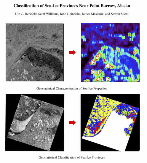
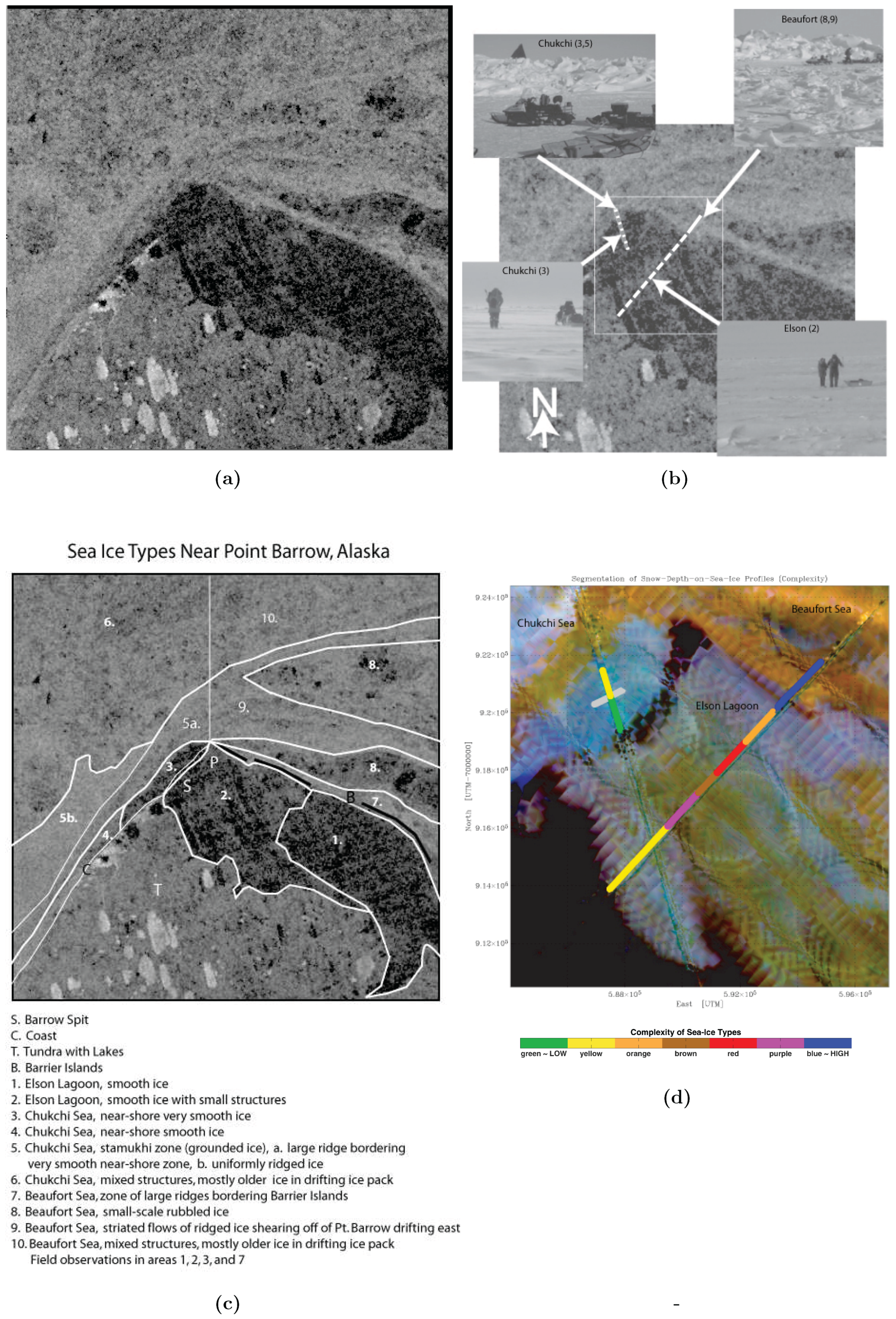
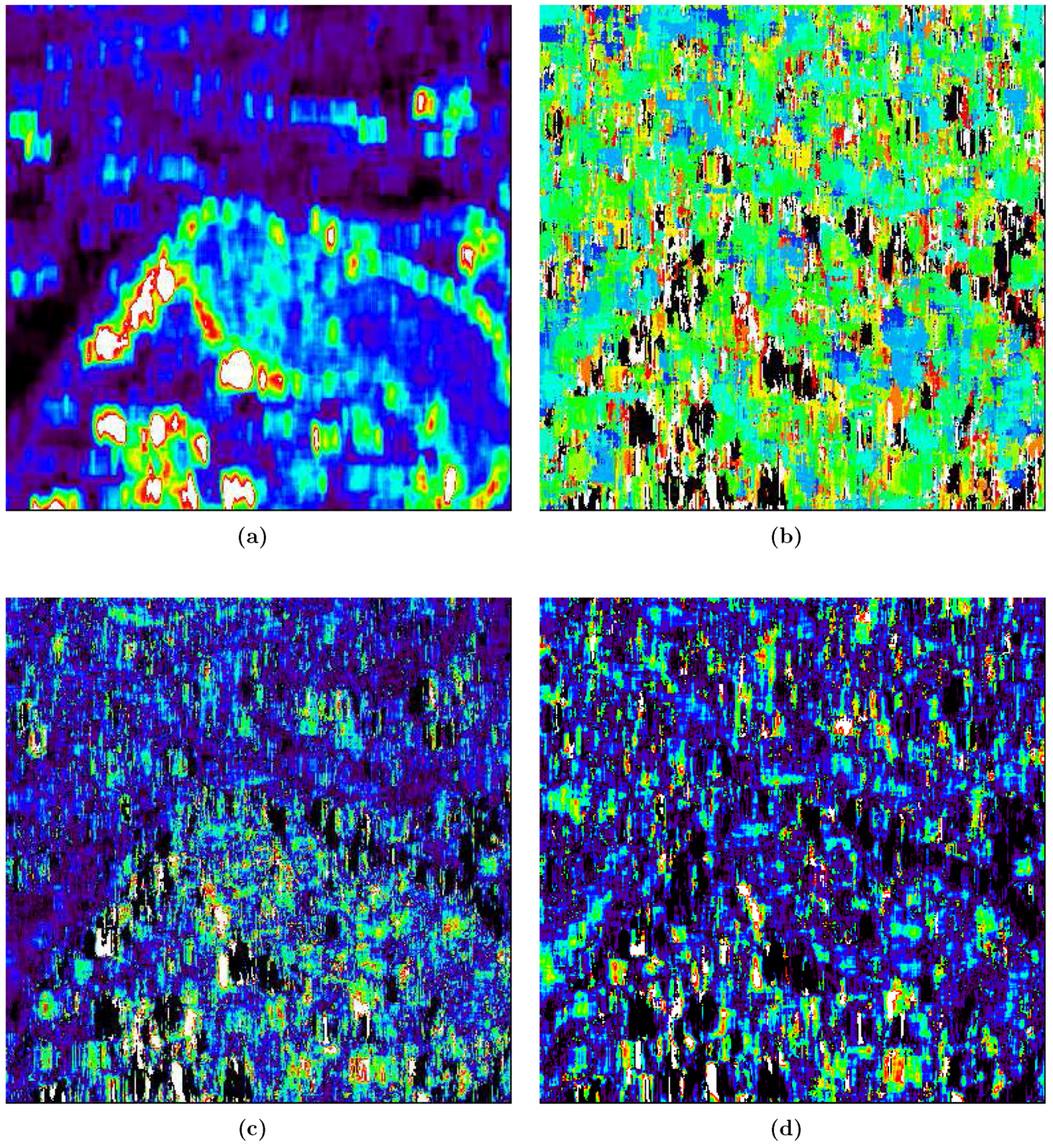
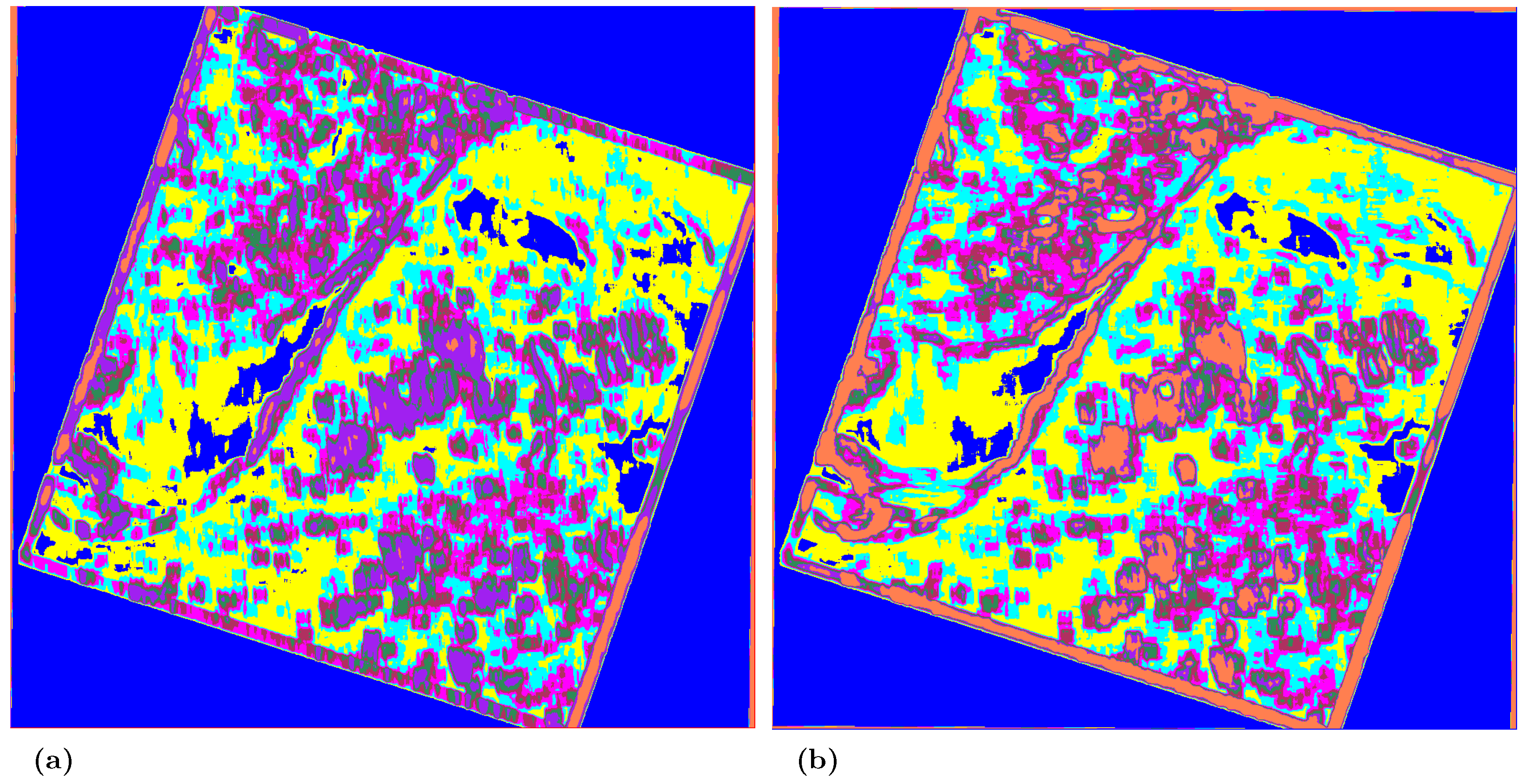