1. Introduction
Radar altimetry was designed to provide highly accurate measurements of sea surface heights over open ocean areas on a global scale. One important application of altimetry is still in the area of oceanography where the datasets help to improve our knowledge of ocean circulation, mesoscale variability, ocean tides, sea level change, etc. [
1,
2,
3]. However, since the launch of the TOPEX/Poseidon satellite in 1992 alternative application areas are grown and nowadays, satellite altimetry is also used for the determination of ice sheet elevations and inland water level monitoring (e.g., [
4,
5]).
In contrast to open ocean altimeter measurements, reflected radar echoes (so-called waveforms) from other surface types show different shapes depending on the reflectors within the altimeter footprint. A careful data editing and reprocessing is required in order to derive reliable and highly accurate range measurements from the received waveforms—a process called retracking. Within the last decade, various investigations on new retracking algorithms have been made in order to enhance the accuracy of coastal and inland water level estimation. In particular, progress has been made regarding lakes and reservoirs (e.g., [
6,
7]) and large rivers (e.g., [
8,
9,
10]). Actually, at least four global databases exist providing inland water level time series for a variety of water bodies based on several altimeter missions [
11,
12,
13,
14]. Their results are highly valuable for applications in continental hydrology, especially given that other data sources such as in situ gauge stations are rapidly declining since about 1980 [
15].
In addition to water levels, information on the reflectivity of the surface can be derived from satellite altimetry. Over open ocean, the sea state, e.g., wind and waves, can be observed [
16] and over land surfaces, the backscatter coefficient allows for the classification of different reflectors. For example, Papa et al. [
17] used TOPEX/Poseidon dual-frequency backscatter values to investigate different land surface types on a global scale. More recently, Le et al. [
18] extended this study by merging data from different missions (Jason-1, ENVISAT, and Jason-2). For both studies, the spatial resolution is sparse since only global or regional scales are examined.
Using radar altimetry for wetland water monitoring is both: (1) a great possibility for deriving hydrologic information in mostly remote areas where in large parts infrastructure is missing and no in situ observations are available and (2) a challenge for data processing as only small areas with open water exist that change rapidly with time. Investigations using radar altimetry to study water level variations of inundation areas and wetlands are rare. Smith and Berry [
19] presented selected water level time series for various wetlands, among them the Pantanal. Their results are promising but a comprehensive validation of the results is missing. Moreover, some dedicated studies exist for the Louisiana wetlands (e.g., Lee et al. [
20] and Khajeh et al. [
21]) and Poyang Lake watershed [
22]. Most of these studies do not provide satisfying results or lack comprehensive validations. In addition, some studies focused on rivers or river basins including inundation areas (floodplains) (e.g., Birkett et al. [
23] and Frappart et al. [
24], both using TOPEX/Poseidon data in the Amazon basin.). The backscatter of radar altimeters was already used to study the variability of wetland extent as shown for example by Zakharova et al. [
25] and Papa et al. [
26]. However, due to the measurement geometry along separate profiles a complete coverage of the area is not possible. Other remote sensing techniques such as optical or radar images are more straight forward. Nevertheless, the altimeter backscatter information is a valuable input for classifying inundation areas beneath the satellite track and may help in fine-tuning the processing parameters to derive water levels from altimetry.
Focusing on the example of Pantanal, the present study investigates the capability of radar altimetry to monitor water level variations of large inundation areas. The backscatter information is used to classify different inundation areas and to define water returns in order to perform a rigorous data editing. The Pantanal is one of the largest wetlands worldwide. It is located in South America, mostly in Brazil with smaller parts in Bolivia and Paraguay. Several interesting studies exist on this inundation area, mainly dealing with the extent of water areas and consequences for the ecosystem, among them Hamilton et al. [
27], Hamilton et al. [
28], Evans et al. [
29], Evans and Costa [
30], Girard et al. [
31], and Padovani [
32]. All these studies rely on sparse in situ gauging stations to derive water level time series. As far as the authors know, no dedicated and comprehensive study on using radar altimetry for estimating water levels within the Pantanal exists.
This study proposes an innovative processing method based on automated altimeter data selection by waveform classification and a dedicated waveform retracking. The results are carefully validated and analyzed region-wide in order to detect spatial patterns of water level changes. The paper provides the first comprehensive study on the use of radar altimetry for estimating water level variations within the Pantanal. However, the focus of the study is not on applications and management of the Pantanal region but on the methodology and assessment of ENVISAT quality in inundated regions.
The paper is structured into four main parts: First, the study area and the used datasets are introduced (
Section 2). Afterwards, the data in the study area are analyzed concerning their capability to detect inundation areas (
Section 3.1) as well as with respect to the spatial coverage (
Section 3.2).
Section 3 also presents the strategy for defining observation points (virtual stations).
Section 4 describes the method used for the computation of water level time series. The results are analyzed and discussed in
Section 5.
3. Inundation Patterns and Definition of Virtual Stations
Due to the satellite’s orbits a complete coverage of the whole area is not possible. Only a few dedicated profiles can be measured. However, the spatial resolution along these profiles is extremely high. A challenging task is the localization of open water areas and the definition of virtual stations. Since the inundation area changes significantly with time and most regions are not continuously covered by water it is difficult to define distinct measurement points. Moreover, the intention of this study is to catch as much information as possible and to derive water levels also for occasionally flooded locations.
Usually the definition of virtual stations is done manually or by using a map, e.g., Google Earth imagery [
8]. This is difficult or even impossible in wetland areas due to small-scale temporal water fluctuations. However, the altimeter instrument itself already provides some information on the reflectors within its footprint. The altimeter waveforms may be classified to separate different surface properties (e.g., Desai et al. [
41]). As an alternative, derived quantities such as the radar backscatter can be used.
3.1. Inundation Pattern Along the Satellite Ground Tracks
The radar echoes as measured by the altimeter can be used to extract information on the properties of the reflecting Earth surface. This can be done directly based on the waveforms or by interpretation of derived quantities such as the backscatter coefficient
. The latter method is the easiest way since one can use the given data sets and an own reprocessing is not required.
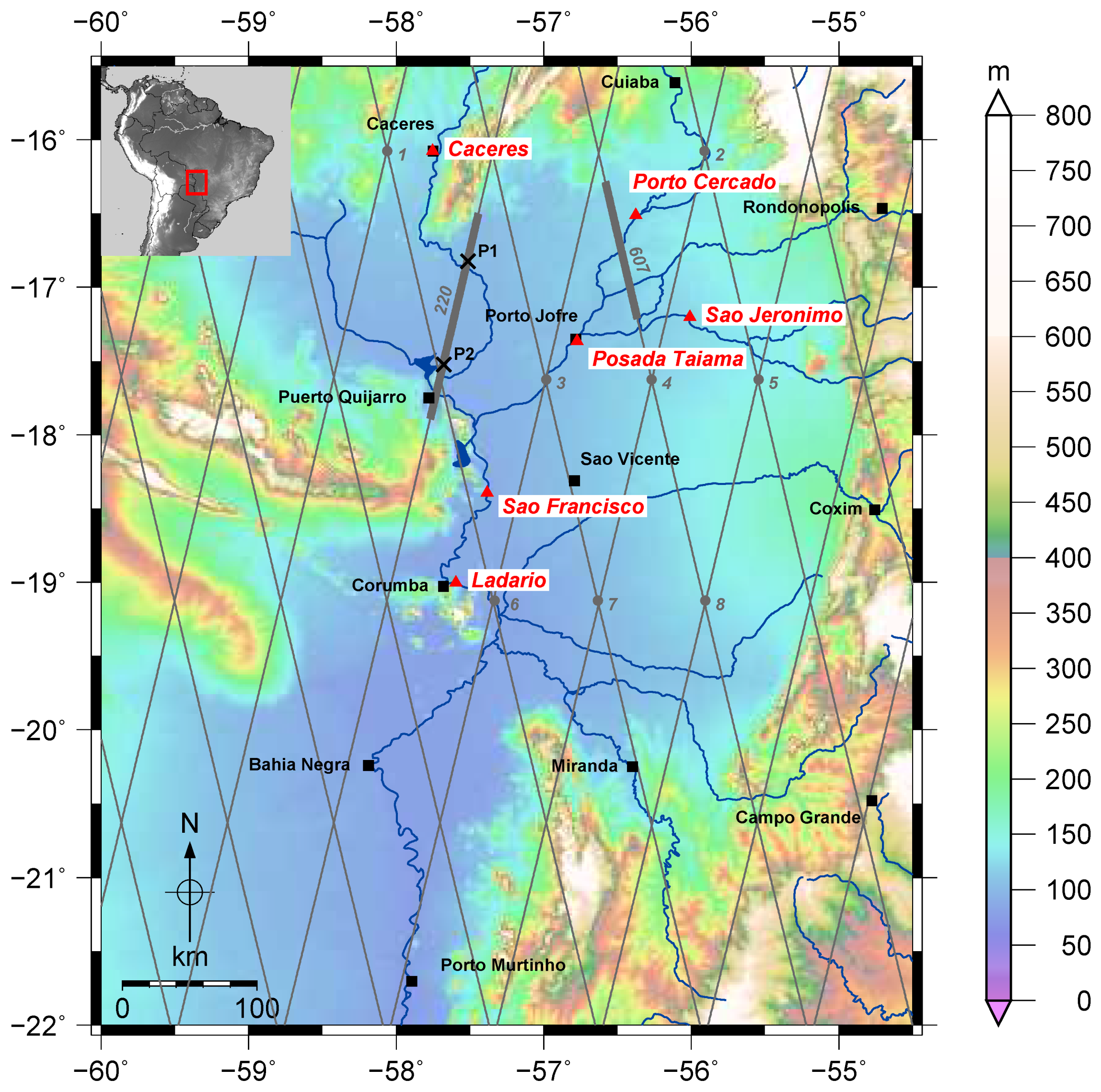
Figure 2 shows the Ku-band backscatter from ice-1 retracker for a short part (about 100 km) of one ENVISAT track (pass 607; location highlighted in
Figure 1). By defining a threshold (in this case 32 dB is used) one can classify measurements with large backscatters as water return with specular reflections [
23]. However, as can be seen from the negative values in the figure, the absolute level of the given values is not correct. Moreover, a direct comparison with other missions is not always possible. That is the reason for using waveform properties for the classification. In this paper, a combination of various waveform parameters (such as peakiness and maximum power) is used to define water returns (more details in
Section 4.1). The results are very similar to the backscatter-based classification.
In
Figure 2 one can define some points along the track with permanent open water (rivers), since they show high backscatters over the whole time span. For other areas periodic changes of backscatter can be seen indicating regions with seasonal flooding. The location of rivers classified by the altimetry backscatter is in good agreement with the rivers provided by HydroSHEDS [
42]. Only one river (at latitude −16.88 degree) cannot be seen by the altimeter. It is not located in a valley and probably very small. It is also not part of the CIA World data bank (WDB II) as used e.g., by Generic Mapping Tools (GMT) [
43]. However, this example illustrates that ENVISAT is able to detect rivers and small open water areas without additional external information.
Thus, radar altimetry can be used to map the temporal variability of water areas in wetlands and to provide information on flood frequency and flood duration. In hydrology, different (non-tidal) wetland types are defined based on their hydroperiods, i.e., the percentage of time that water is standing. In U.S. EPA [
44], seven types are listed based on the general relationship between wetland water levels and hydric states. It is difficult to group the altimetry results into the seven original classes as long as the flood duration is not analyzed in detail. In this study, a classification into four groups is performed based on the percentage of water returns per track segment over the whole time span. This defines the inundation frequency for the different areas. If altimetry detects water in less than 20% of the time, the segment is classified as “mostly dry”. In cases where water is in the segment for up to 50% of the time, the segment is “temporarily flooded”. This class also incorporates “intermittently flooded” areas. An area is defined as “seasonally flooded” when water is detected for 50% to 90% of the time. At last, a segment is “permanently flooded” in case water is present in more than 90% of the time. The definition of the four classes used is summarized in
Table 2. Naturally, the class limits are somehow arbitrary, since a distinct separation is hardly possible.
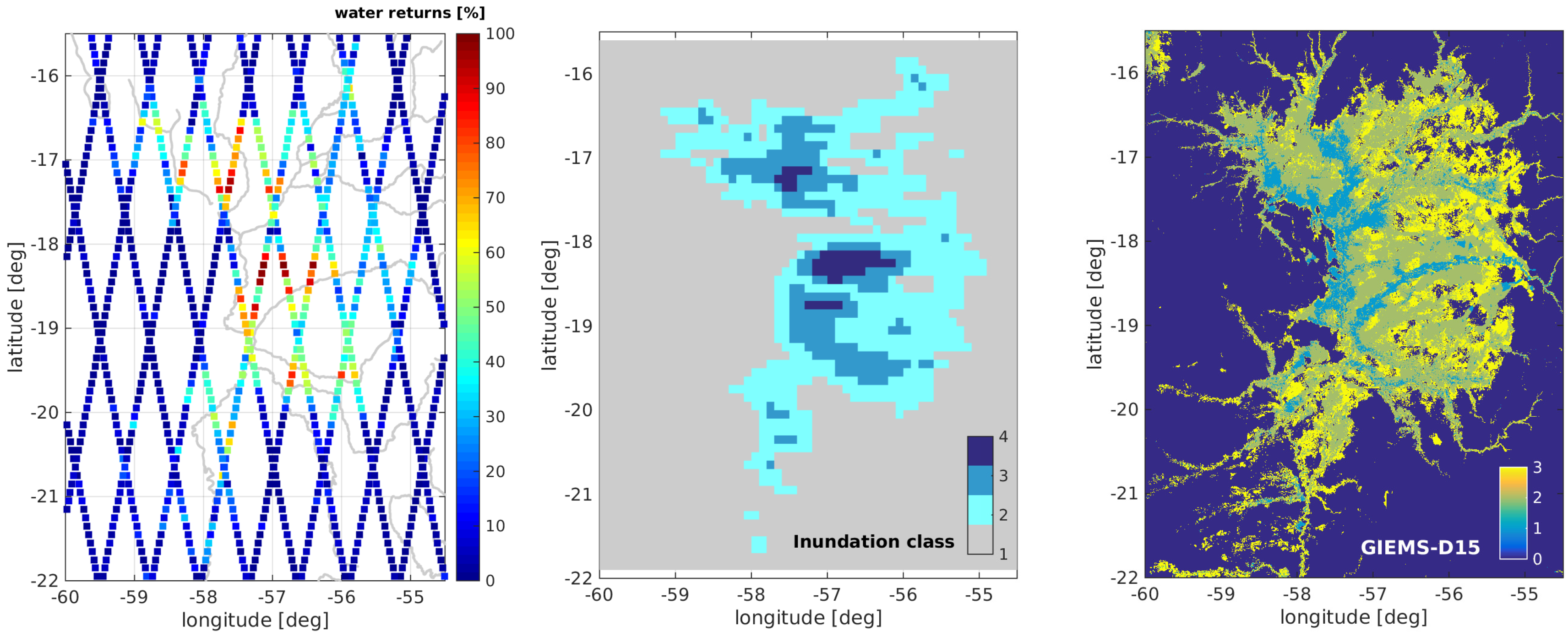
The corresponding classification results are shown in
Figure 3. The left part of the figure shows the percentage of water returns in small track segments and the middle part displays the derived inundation classes. One can clearly identify the extent of the wetland even if no external information on the boundaries are used to generate these plots. In addition, areas with open water throughout the whole years can be identified: one around the Rio Paraguay South of Caceres and another at the lower Rio Taquari around 100 km North-East of Corumba. On the right-hand side of
Figure 3 an external classification from GIEMS-D15 [
45,
46] is provided showing three states of inundation extent. As these results are mostly based on satellite images, they cover the whole Pantanal area. The spatial resolution of about 450 m is the same for both data sets, however, the time periods differ significantly: while GIEMS-D15 is based on data between 1993 and 2004 the altimetry data are from 2002–2011. Moreover, the inundation frequency is not necessarily directly connected to the inundation extent. This might explain some of the differences visible mainly in the central part of the Pantanal. ENVISAT classifies large parts west of Sao Vicente and north of Rio Taquari as open water whereas in GIEMS-D15 mainly the Rio Taquari itself is visible. Since this region is characterized by many small rivers and small areas of standing open water it is not clear why it is not visible in GIEMS-D15. Similar discrepancies can also be seen comparing GIEMS-D15 with MODIS-based results from Padovani [
32] as presented in Fluet-Chouinard et al. [
45] (
Figure 7, page 358). Moraes et al. [
47] also reported open water between Sao Francisco and Sao Vicente.
3.2. Definition of Virtual Stations: Track Segmentation Concept
Radar altimetry can only provide water levels when the satellite’s footprint covers open water. In order to derive water level times series of inland waters so-called virtual stations (e.g., [
48]) are defined at locations where the satellite track crosses a lake or a river. Classically, this is done using given time-independent water body maps or remote sensing images. Since the inundation pattern within wetlands changes rapidly from one location to the next, it is challenging to define virtual stations offside larger rivers and lakes. However, these are the most interesting regions since no in situ datasets exist.
Instead of selecting single virtual stations all satellite tracks are separated in regular pieces of 0.05 degree (corresponding to about 6 km) and each of these track segments define one virtual station. This ensures around 17 measurements per segment and overflight. The segmentation size is a compromise between a good data coverage and a high along-track spatial resolution. Small segments ensure homogeneous conditions within the single compartments, e.g., similar hydrological conditions and no terrain slope. Since clearly not all virtual stations will contain open water a careful data pre-processing is necessary in order to get rid of land-contaminated observations (see
Section 4.1).
Due to the sparse cross-track spatial resolution of satellite altimetry some regions will be missed even when using more than one repeat-track mission. This is related to the nadir measurement principle and the orbits of satellite altimetry and cannot be avoided.
The location of crossover points (where ascending and descending passes are crossing each other) can be used to perform a validation (see
Section 4.4.1).
4. Computation of Water Level Time Series
For each 0.05° track segment one time series of water level is computed. For this purpose, a careful data pre-processing is required since the data quality over inland water targets is not as good as over open ocean. Especially waveforms contaminated by land should be excluded from computations. Moreover, a dedicated retracking is recommended in order to increase the data quality.
For many applications the derivation of accuracies along with water levels is valuable. Thus, an error information for each water height is derived in addition to the water level itself.
4.1. Waveform Classification
Since the definition of virtual stations is done automatically and not only in permanently flooded areas, not all altimeter measurements are usable. Due to the diversity of reflecting surfaces (e.g., open water, swimming vegetation, flooded areas covered by vegetation, land,...) the altimeter waveforms show a rich variety and different qualities. The elimination of unusable data from the processing is realized by waveform classification.
This is done by applying selected thresholds on waveform-related statistical parameters such as skewness, kurtosis, peakiness, maximum power, and signal-to-noise ratio. The method divides the altimeter returns into four major classes, one of them called “single peak” containing pure quasi-specular waveforms as returned from small inland open water reflectors. This is the only class used in this study. Thus, the identification of the other classes is not discussed here. The identification of the quasi-specular waveforms is based on the normalized peakiness that is computed from the waveform power
for
and
by dividing the maximum power of the waveform by the sum of the waveform power following Equation (1).
A threshold of 0.5 is defined to identify inland water reflectors.
Figure 4 shows two waveform examples registered over inland. On the left-hand side a specular waveform with a peakiness of 0.53 is plotted. The right-hand side displays a corrupted waveform (peakiness of 0.04). In this study, only waveforms with peakiness parameters larger than 0.5 are used. This implies the rejection of ocean-like returns. Thus, larger water bodies such as major lakes cannot be covered by this approach.
4.2. Retracking
All remaining waveforms classified as inland water returns are retracked in order to derive precise altimeter ranges and water heights. For this purpose, the altimeter waveforms are analyzed in order to extract the travel time of the signal coming from the main reflector. For ocean waveforms this is defined by the mid point of the waveform’s leading edge. For specular waveforms it is the waveform’s peak location itself. In order to avoid the use of different retrackers and problems with unknown retracker biases [
49] only one retracker is used for all waveforms. To be more precise, an improved threshold retracker [
50] is applied. It uses the subwaveform with the most pronounced peak to derive the range and a threshold of 100%, i.e., the location of the peak itself. This is possible since only specular waveforms with one dominant peak pass the classification (cf.
Section 4.1).
Since the retracking is not performed analytically or by fitting a function to the waveform it is not possible to estimate an error information for each retracked range. Consequently, no range accuracy can be computed based on the retracking. Therefore, an alternative method for the generation of the water level error per overflight is necessary.
Before computing the water level time series, each retracked range has to be corrected by the ordinary geophysical corrections (cf.
Section 2.2). Moreover, normal heights are computed using the satellite’s height and a geoid model. The measurements and models used are listed in
Table 1.
4.3. Generation of Water Levels and Error Information
Since the pre-processing yields a precise and reliable dataset without many outliers the computation of water level time series can be done with a simple median approach. All pre-processed observations from one track segment are used to compute the median of heights as well as a standard deviation to represent the precision of the derived water level.
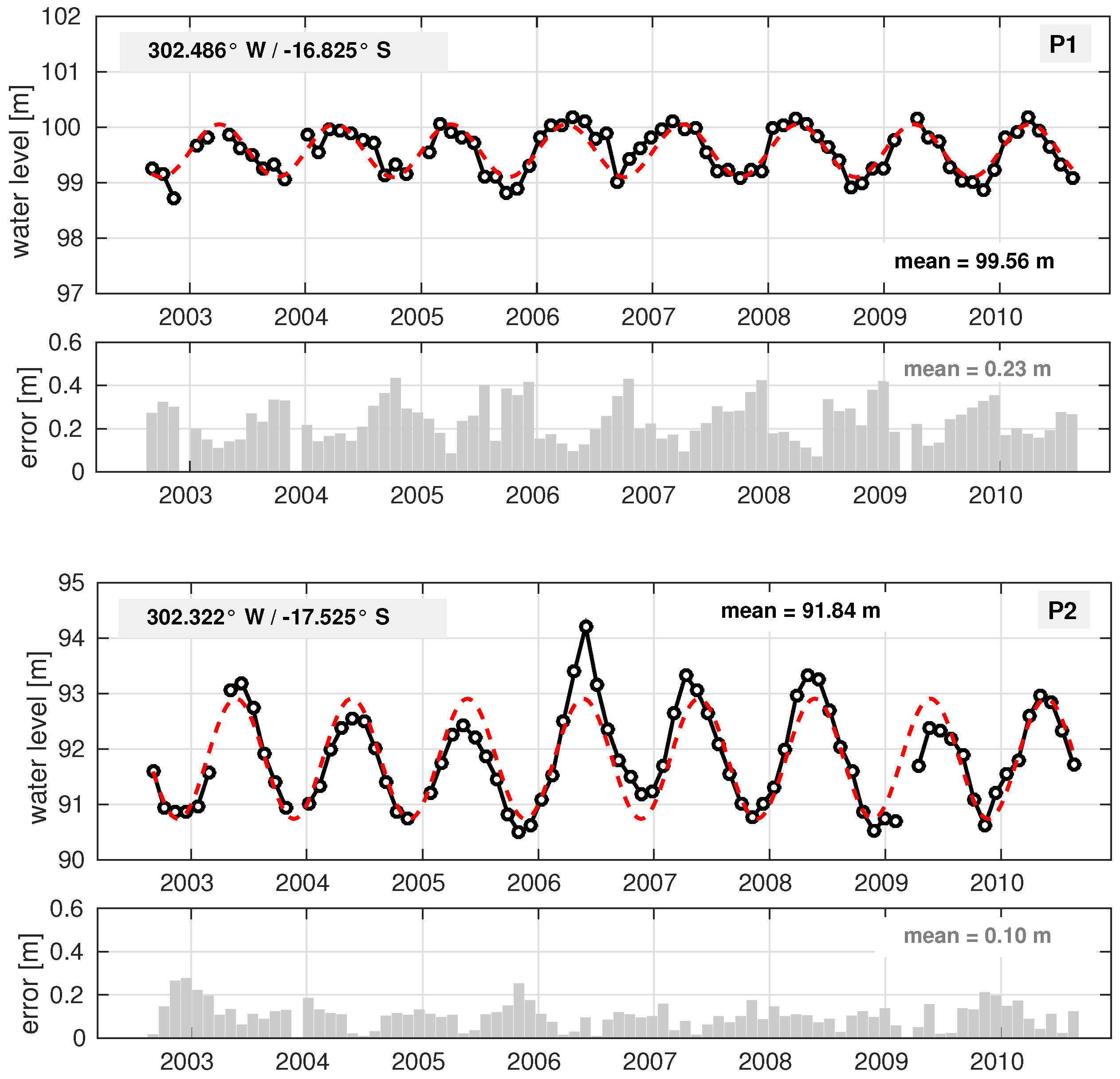
Figure 5 shows two example time series computed for two different locations along ENVISAT Pass 220, both classified as inundation class 3 or 4 (permanently or seasonally flooded). The northern station is located in the floodplains of Rio Paraguay whereas the southern station lies near a smaller river called Corixo do Guira. The locations of both stations are indicated by black crosses in
Figure 1.
Both stations show different flooding behavior. The first location shows a regular annual variation with an amplitude of 0.47 m and maximum water levels around February/March. The second station has larger variations with a mean annual amplitude of 1.08 m. Here, the epoch of the maximum water level differs significantly between years. In most years, the maximum water level is reached later than in the case of the northern station (around April). The standard deviations computed along with the median from all water heights within one track segment (denoted as error in
Figure 5) are larger for the northern station –probably due to smaller water extent. Both error time series show a negative correlation with the water level, thus, the errors are larger in the case of lower water levels.
The use of more advanced processing such as implemented in the DAHITI software [
14] can slightly improve the quality of the time series. However, for most track segments, this computation effort is not worthwhile.
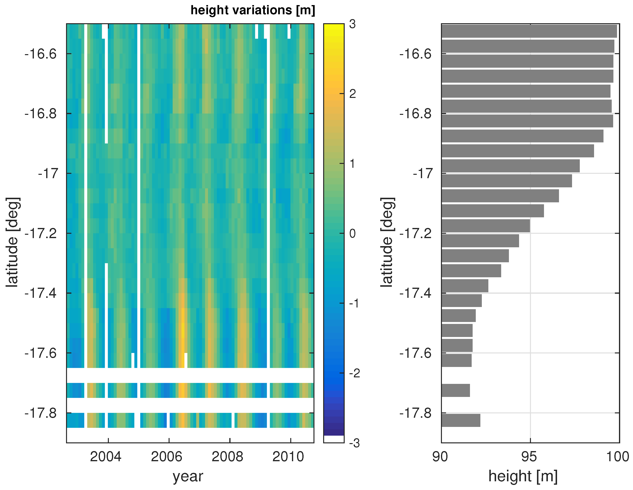
Figure 6 displays a part of Pass 220 between −17.9 degree and −16.5 degree latitude. The geographical location of the track can be seen in
Figure 1. The plot summarizes results of 28 track segments, 78.6% of them in inundation class 3 or 4. For a minority of stations, only land returns or no valid data is available and visible as white spots in the plot.
4.4. Validation
As described before, for each water level an error estimate is computed in order to provide information on the quality of the heights. The mean standard deviation of all time series at locations in inundation class 2–4 (at least temporarily flooded) yields 0.4 m with 94.6% of the values below 1 m. Neglecting the outliers an average precision of 0.3 m can be reached. The best time series shows a mean standard deviations of 7 cm. These error estimates are in the same order of magnitude with the quality documented for permanent inland water bodies [
14].
Now it has to be checked whether these formal errors really represent the accuracies of the time series. Usually this validation is done by a comparison to external and independent datasets. However, in remote areas such as the Pantanal only sparse coverage with in situ gauging stations exists.
Before doing the validation, the uncertainty of water levels will be evaluated by comparing time series at crossover points, thus, between ascending and descending passes of one mission. Even though these comparisons cannot reveal any information on the external accuracy of the time series, the internal accuracy (or precision) can be estimated.
4.4.1. Comparisons at Crossover Points
In the study area a few crossover points between satellite tracks are available. These locations can be used to compare the time series originating from different tracks or different missions. When doing so it has to be taken into account that the observations neither cover exactly the same locations (as they are measured on 6 km long inclined tracks) nor the same times. Nevertheless, the comparison reveals interesting information on the uncertainties of the time series.
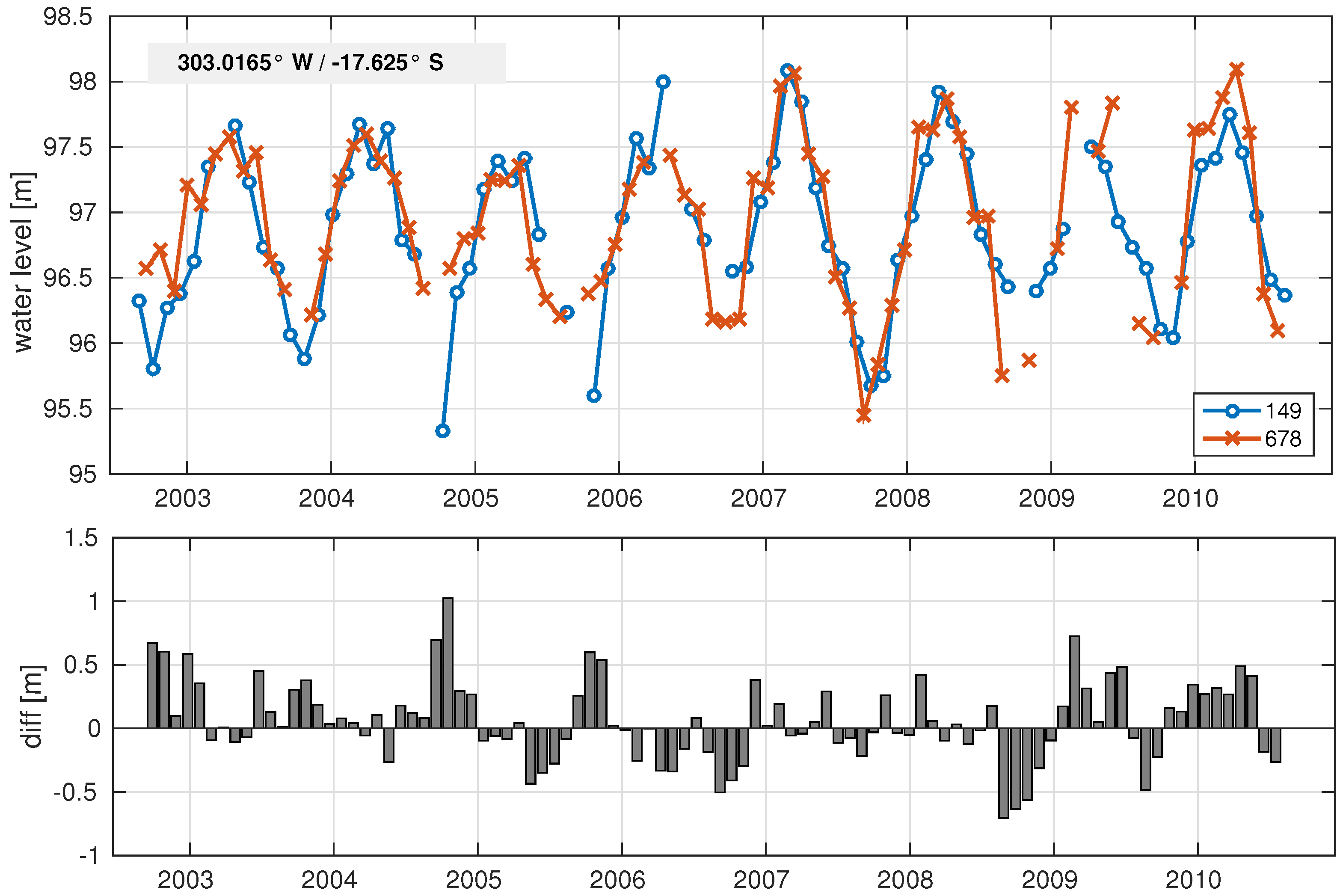
From the 18 ENVISAT passes within the study area 30 crossovers can be built. However, most of them are located in inundation class 1 (mostly dry). Only at eight crossover points both tracks have enough water returns to allow for reliable time series estimates. The locations of theses crossover points are highlighted in
Figure 1. Comparing the respective time series, correlation coefficients (R) between 0.42 and 0.94 are obtained with root mean square (RMS) differences between 0.7 m and 0.3 m. The results from all crossovers are given in
Table 3. The best agreement is reached at the crossover point 6 in inundation class 3, even if only 74 points of the time series can be used for the comparison (#, last column).
Figure 7 shows the two time series for crossover point 3 and their differences. Even if differences of about 1 m are visible, the RMS difference of 32 cm is acceptable and in the same order of magnitude with most river crossings [
14]. The mean standard deviation of the time series is 0.28 m for pass 678 and 0.25 m for pass 149, respectively. Thus, the standard deviation of the difference
can be computed with 0.38 m. This is similar to the RMS difference and this result shows that the formal errors of the time series well reflect the precision of the data. This holds for all validation points (cf.
Table 3).
4.4.2. Comparison with in Situ Gauging Stations
Since a comparison of time series in crossover points can only reflect the precision of the datasets and not their realistic uncertainty a comparison with external validation data is necessary. This is normally done by using in situ water level measurements of gauging stations. Unfortunately, the number of gauges in remote areas is limited. Moreover, gauges are only installed at permanent water bodies such as rivers or lakes and do therefore not reflect the water levels of inundation areas. However, due to a lack of alternatives, river gauges are used for the validation here. The comparison is done using the nearest ENVISAT track crossing of the same river and the track segment that covers most of the river. Thus, due to the segmentation concept (
Section 3.2), the altimetry data used for processing the time series is not directly located above the river and can also comprise river floodplains. Moreover, a validation of time series offside larger rivers is impossible.
Within the Pantanal, data of about 25 river gauging stations are provided by Ag
ência Nacional de
Águas [
51]. After rejecting all datasets that do not overlap with ENVISAT over more than one year only six stations remain in the central area of the Pantanal with measurements starting in 2005. They are distributed along three different rivers in the region. Since all six in situ time series are of minor quality (especially in the first years) and show a lot of outliers and unreliable data points a rigorous data screening is required. This is performed based on daily data sets by means of a 3
σ-outlier test (taking annual variations into account) and a manual post-processing. The amount of rejected outliers varies between 3.5% for station Posada Taiama and 23.8% for Porto Cercado.
Table 4 summarizes the comparison. In addition to information on the gauge (station name, river, and location), the distance to the altimetry target and the ENVISAT track number are provided. A large distance will for sure have a negative influence on the similarity of the time series since the conditions at the two locations cannot assume to be equal. It is worth mentioning, that the distance is computed from a straight line to the next ENVISAT crossing of the same river. The distance along the river will be much longer in most cases. The last three columns of the table show some statistics from the time series comparisons (RMS difference, correlation coefficient R, and number of points for the comparison). With one exception, the RMS differences are between 30 and 50 cm. These values are in the same order of magnitude with the results from the crossover analysis (
Section 4.4.1) and the formal errors of the altimetry time series.
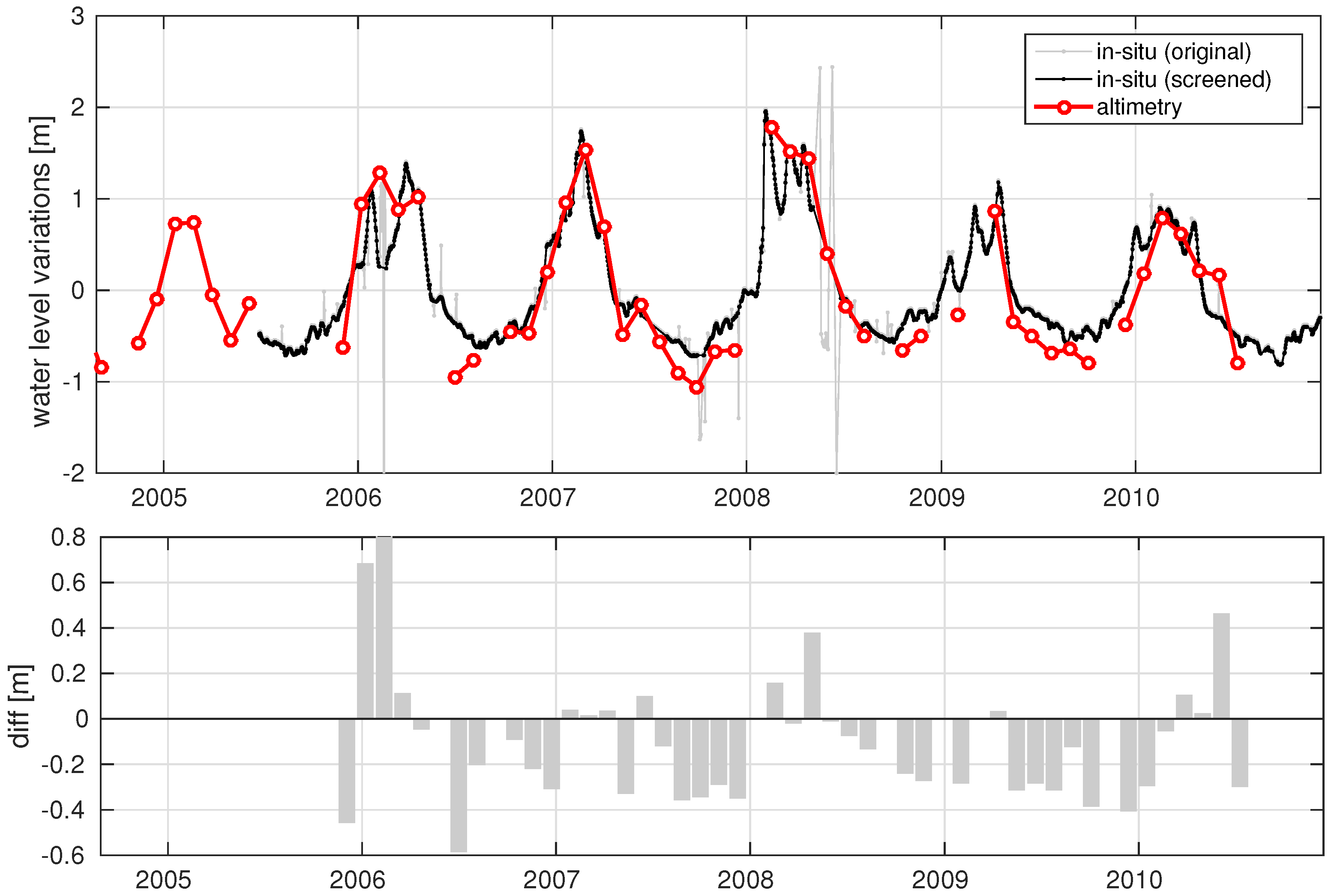
Good agreement between altimetry and in situ data is observed for station Sao Jeronimo at the Rio Piquiri. Here, the distance to the nearest altimeter track segment close to the river is around 17 km upstream. Moreover, there is almost no meander between the two locations and similar conditions can be assumed. The two time-series are shown in
Figure 8.
They have about five years overlapping time for comparison. Since the absolute level of the in situ data is unknown, both time series are reduced by their means and only height variations are compared. Due to the different temporal resolutions the in situ data were interpolated to the altimeter time tags and 42 data points are compared. The RMS differences yield 32 cm with the largest differences during the low water periods. This is in line with the formal errors of the altimeter time series (see
Section 4.3). It should be considered, that the altimetry time series is not computed directly over the river but at the nearest track segment defined in
Section 3.2. Thus, they cannot optimally represent the river. This will add an additional error contribution to the uncertainties of water level measurements of altimeter and gauging station. Keeping this in mind, an accuracy of 30 cm is very good, since it is in the same order of magnitude with results for dedicated river time series [
10,
14].
In order to evaluate the quality of the water level time series, the RMS should be related to the height variations itself. In case of larger variations, a higher RMS is acceptable since the variation is still well depicted. Thus, for the areas with small water level amplitudes of only a few decimeters the accuracies are within the range of the signal itself. Here, an interpretation of the results is difficult.
5. Interpretation and Discussion
In the previous section single water level time series and their accuracies have been analyzed. Now, all valid datasets will be exploited together in order to allow for an interpretation of the water dynamics within the whole Pantanal. However, in order to get reliable results it is important to use only those time series that are trustworthy and of high precision. Thus, for all further analysis only time series fulfilling three criteria will be used: (1) percentage of water returns larger than 20% (at least occasionally flooded); (2) number of valid points in time series larger than 50 (about half of the theoretically possible epochs); and (3) mean formal error
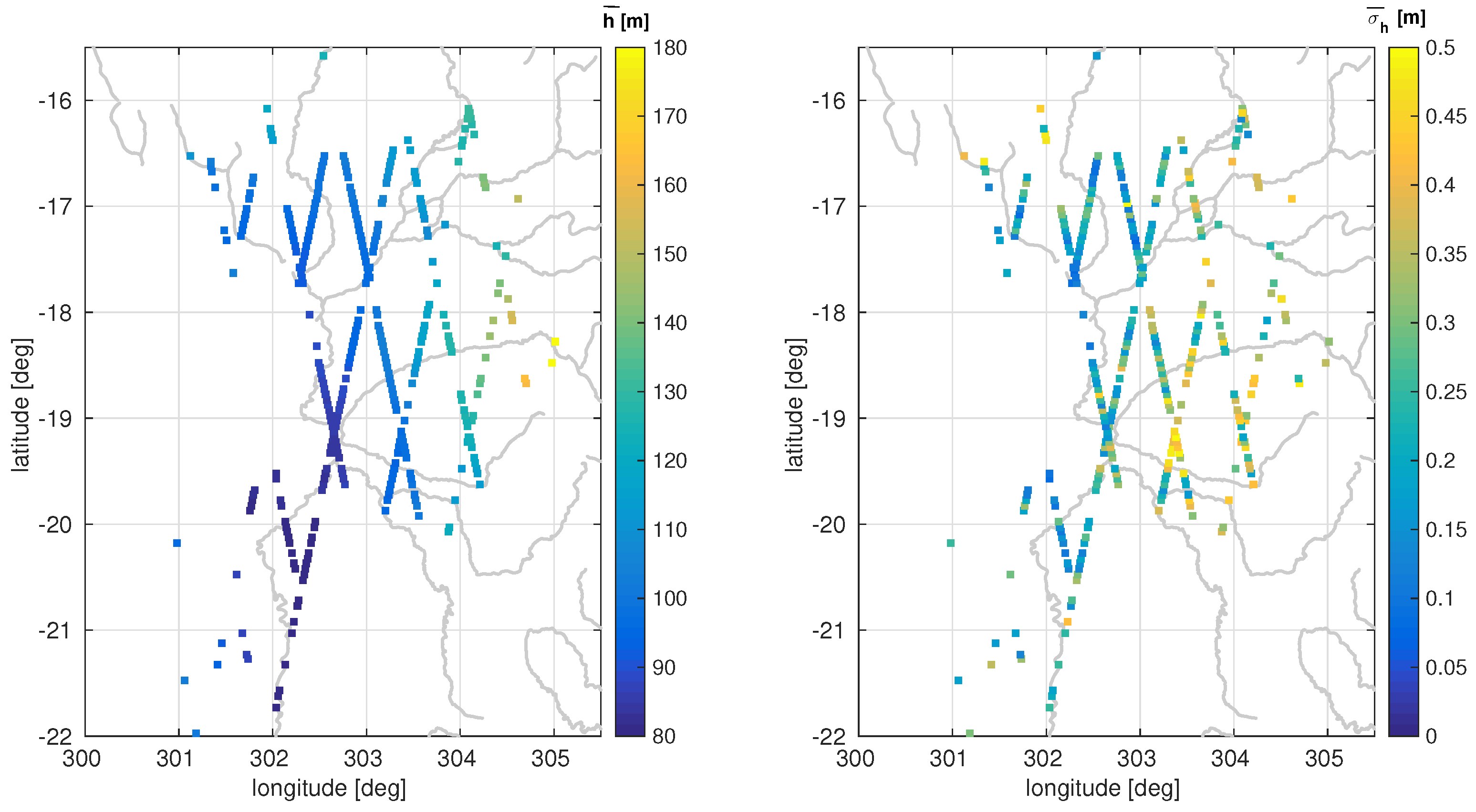
smaller than 0.5 m (78% of all valid time series). The remaining number of time series is 336, about 17% of all possible track segments in the study area. Most time series (70%) are rejected because they are located above mostly dry terrain (inundation class 1, first criteria). The averaged height of each point and its mean formal error is plotted in
Figure 9. On the left-hand side one can see the basic topography of the region with decreasing terrain from North-East to South-West and the lowest part around the Paraguay river. This structure can also be seen in the error estimates (right-hand side) but with much more noise due to local conditions.
5.1. Harmonic Fitting
The common interpretation of all time series is demanding since the local conditions differ significantly from each other and the time series show quite different behavior. In order to analyze the results the time series are represented by harmonic functions. A fitting by linear or spline interpolation is not used because they produce unreliable results in the case of data gaps that are frequent in the time series, especially in areas that are only occasionally flooded.
A Fourier Series is fitted to each time series using Equation (
2) with six terms (
), i.e., 13 unknown parameters are estimated representing one constant (describing the mean height), six amplitudes, and six phases. The fundamental period of the function is fixed to one year (
) in order to represent seasonal variations.
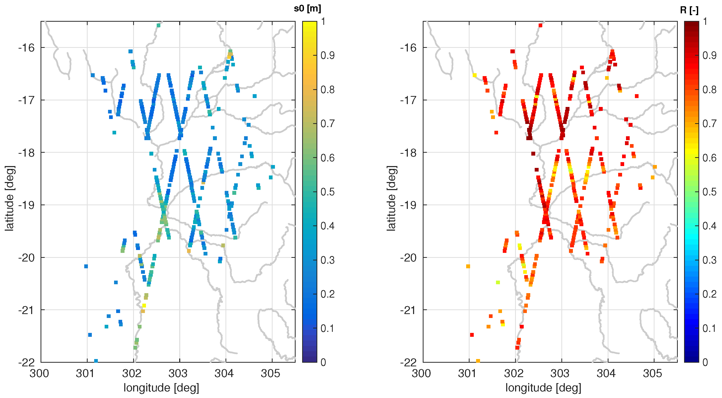
In order to judge the quality of the fitting and to decide if the water level can be described as a harmonic function, the standard deviation of the fit
and the correlation coefficient
R between time series and estimated fit are evaluated. Both quantities are plotted for all valid time series in
Figure 10.
288 (85.7%) time series can be fitted with
0.5 m and 302 (89.9%) reach a correlation coefficient larger than 0.7. When both criteria are fulfilled it is assumed that the signal can be well represented by the harmonic fit. This is the case for 255 (75.9%) time series, mainly located in the northern part of the Pantanal. For 232 of these stations, the main oscillation has a period of one year. The rest have other dominant periods. These stations are all located in the South of the Pantanal region.
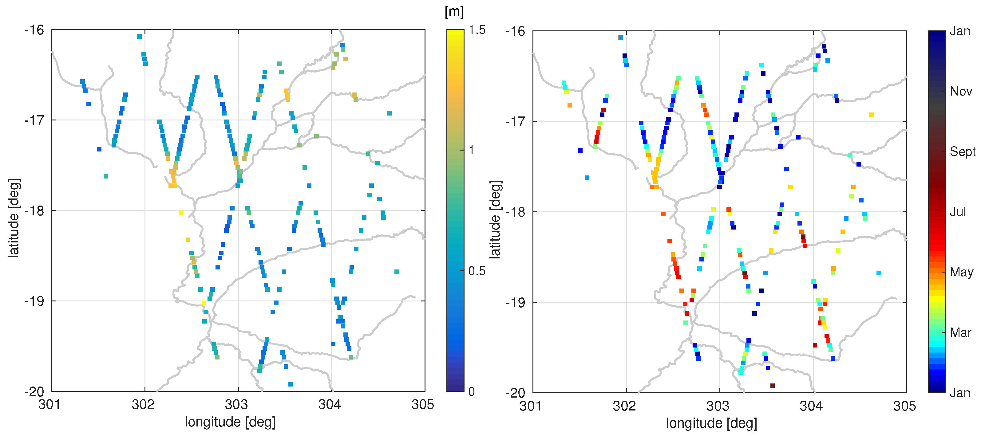
Figure 11 shows the amplitudes and phases of the annual signal (
in Equation (
2)) of each station with a reliable Fourier fit. The estimated amplitudes range between 0.1 and 1.5 m, reflecting only seasonal behavior. The month of maximum water level varies between January and June with only a few time series showing maxima later in the year. Near the Rio Paraguay (flowing from North to South between 302 and 302.5 degree longitude) neighboring track segments are nicely correlated with each other (for both parameters). However, in the East of the study area the phase of the fitted signal show larger point-to-point variations, probably due to the direction of the river flow in this region (nearly perpendicular to the satellite tracks).
Since the annual cycle is only one component of the water level variations a common interpretation of all coefficients of the Fourier fit is straightforward. This can be achieved by means of a principal component analysis (PCA).
5.2. Dominant Patterns
In order to analyze all time series together and to detect dominant modes in the variations a PCA (e.g., Jolliffe [
52]) is applied. For this purpose, the 255 Fourier series from
Section 5.1 are used as input in order to ensure the same time period and discretization for each time series. The mean value (i.e., the mean height, coefficient
c from Equation (
2)) is subtracted from the time series before using the data in PCA since only temporal variations shall be interpreted.
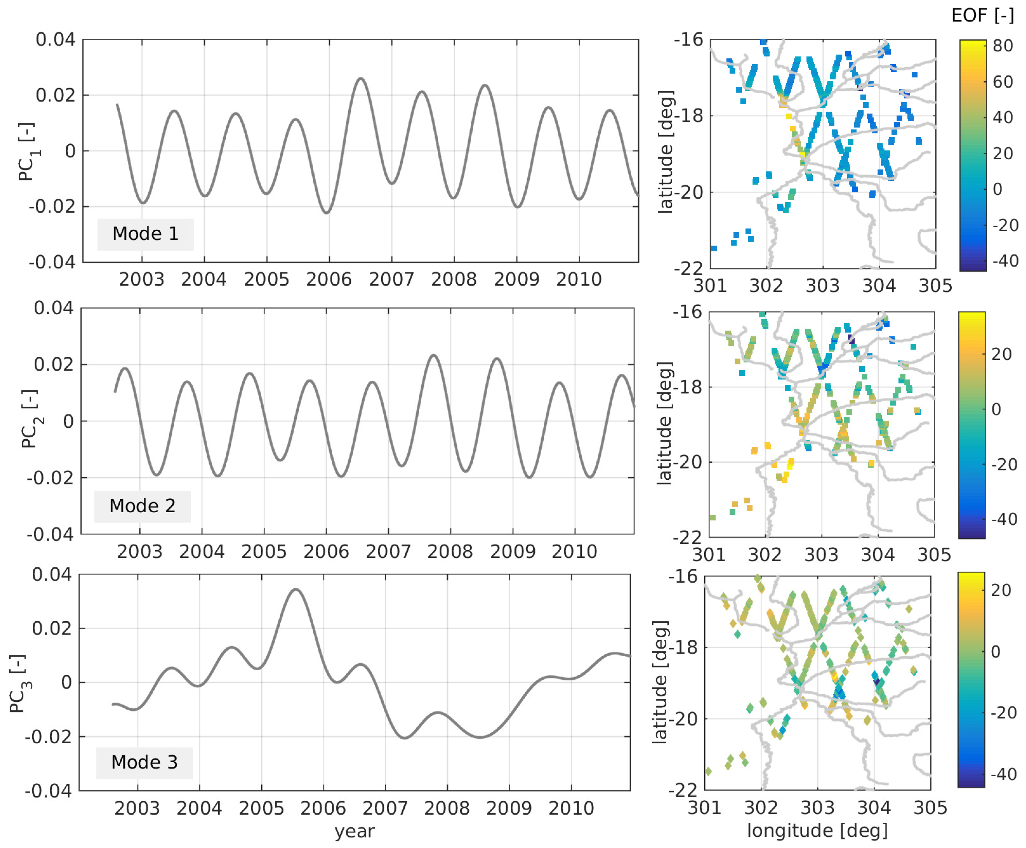
By PCA, spatial-temporal variations can be analyzed based on the covariances between the time series. For this dataset, three modes are required to explain nearly 80% of the allover variance of the system. The relative contribution per mode is given in
Table 5. In order to describe 95% of the signal variance at least 10 modes would be necessary. For this study, the first three modes are used for describing the main spatial and temporal structures of the water level variations of the Pantanal. The resulting temporal and spatial patterns are displayed in
Figure 12. The standard deviations of the residuals per time series remain smaller than 0.4 m, except for single outliers. The first two modes are dominated by annual variations with different phases. The first mode shows maxima in the mid of the year around June, mainly in the central west of the area (northern Rio Paraguay), whereas the second mode represents water maxima in spring (around March) along the Piquiri river (negative values in the spatial plot) and later in the year at the southern Paraguay (positive values). Mode 3 reflects exceptional events focused in the South of the Pantanal along the Rio Negro (mode 3). The stations along the Rio Negro show negative values (drought) before 2007, especially in 2005, and higher water in 2007 and 2008. However, the contribution of mode 3 to the overall signal is very small and should not be overvalued.
5.3. Comparison with Mass Changes Derived from Gravity Recovery and Climate Experiment (GRACE) Mission
In order to evaluate the altimetry-derived water level changes they are compared to mass changes observed by the GRACE mission [
53]. Monthly GRACE gridded land fields [
54] are used to compare liquid water equivalent thickness (LWE) variations with water level variations. The results are based on the solution of GFZ (Deutsches Geoforschungszentrum). However, no significant differences can be seen when analyzing one of the other two solutions.
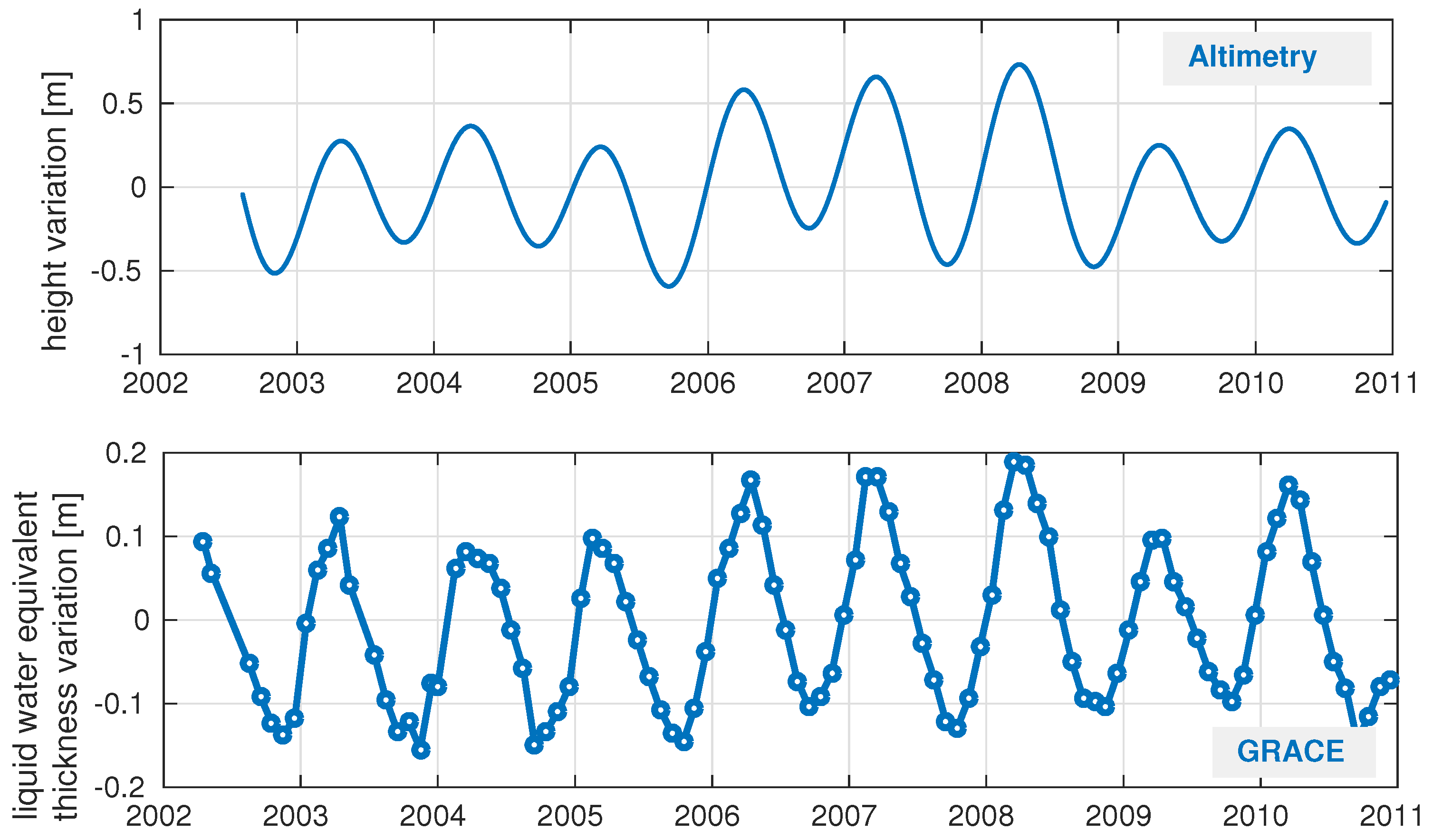
Figure 13 shows the altimetry-derived water level variations (top) and the GRACE-derived LWE (bottom) for the whole study area. The first plot is computed by averaging all time series from
Section 5.2 (as used for PCA). Both time series shows similar variations with a clear seasonality. For the years 2006 to 2008 larger amplitudes can be seen in both time series. The correlation coefficient R yields 0.95. However, the absolute amplitudes differ by a factor of about two. This may be related to two main facts: (1) the altimetry time series do not represent the whole area as they are only provided at dedicated stations; and (2) the GRACE time series is smoothed due to the data sampling and post-processing (e.g., de-striping and filtering) even though the recommended scale factor is applied. Moreover, the measured quantities of the two time series are not directly comparable: GRACE observes total mass changes whereas altimetry can only measure surface waters. Thus, a reasonable comparison is only possible on a relative level without taking the absolute values into account.
In a next step, a PCA is applied to the GRACE dataset (given on a 1-degree grid) in order to analyze the spatial variability of the data.
Figure 14 illustrates the result. The first PCA mode represents 90.8% of the signal, thus, all further modes are negligible and will not be interpreted. Comparing the spatial pattern to the altimetry result (
Figure 12) one can detect some congruences. The largest GRACE amplitudes can be seen in the northern part of the region and along the River Paraguay. This also holds for altimetry even though separated to different modes: mode 1 shows the largest amplitudes along the Paraguay and mode 2 in the northeast (Rio Cuiaba). However, the altimetry results indicate higher water level variations along the Paraguay than along the Rio Cuiaba. Moreover, only moderate amplitudes are visible in the north and northwest. Probably, the high GRACE amplitude in this region is due to other water reservoirs (such as groundwater or soil moisture). Moreover, GRACE seems not able to resolve the different phasing of the surface water since only one seasonal mode is detectable.
Thus, considering the different characteristics and qualities of both observation techniques, both datasets show a good agreement. A combination of both measurement techniques might provide additional information for analyzing different compartments of continental water storage and to separate liquid surface water variations from groundwater or soil moisture. However, this can only be done after transforming the datasets to comparable spatial scales.
6. Conclusions and Outlook
This study demonstrates the ability of radar altimetry for monitoring water levels of inundation areas. The example of the Pantanal region in South America is used to show the possibilities and limitations of this technique to monitor water heights of temporarily flooded areas. Within the test region, the formal errors of the derived water level time series yield about 40 cm on average with best results below 10 cm. The comparison at crossover points and with in situ gauging stations confirms the reliability of the formal errors and gives accuracies between 30 and 50 cm. These values are in the same order of magnitude with results reported for smaller rivers. Water level time series with this accuracy can only be achieved by using a rigorous data editing (by means of waveform classification) and a dedicated data retracking. It is worth mentioning that the results for the Pantanal are not necessarily representative for other wetlands. Since the accuracy of inland altimetry strongly depends on the characteristics of the reflecting surface, varying conditions such as ground level elevations and vegetation cover may lead to different accuracies and thus limit or increase the applicability of satellite altimetry for the monitoring of flooded areas.
Due to its measurement geometry along dedicated satellite ground tracks, satellite altimetry is not able to provide a complete data coverage of the Pantanal. Even though a high along-track resolution of a few km is possible, the cross-track resolution depends on the orbit of the mission(s) used. This study is limited to ENVISAT data. The use of additional missions such as Jason-2 or Sentinel-3 might improve the spatial (and temporal) data coverage. Of course, altimetry can only provide water levels if the area within the footprint is partly covered by water – at least for a certain period of time.
Since it is not possible to use a constant land-water mask to define flooded areas, external datasets are necessary. This study uses the altimetry returns themselves to identify open water returns: waveform classification or backscatter analysis show similar results and are both suitable for this purpose. A separation of the Pantanal in four inundation classes based on altimeter waveform classification shows a good agreement to classifications based on imaging data (GIEMS-D15).
Using altimetry, seasonal water level variations as well as particular events can be detected. It allows for analyzing floods in space and time. For the Pantanal, most areas show a clear annual cycle with maximum water levels between January (north/east of the region) and June (south). The amplitudes can reach up to about 1.5 m for larger rivers and their floodplains. However, substantial areas of the Pantanal show smaller water level variations (only a few decimeters), which are in the same order of magnitude with the accuracies of inland radar altimetry. For these parts of the Pantanal, no reliable water height information is extractable. Further investigations are necessary to improve the results in these areas. The usage of delay-doppler altimeter data (such as measured by the recently launched Sentinel-3 mission) might improve the along-track resolution and the extraction of water returns in vegetated areas.
A combination of altimeter-derived water levels with surface water extent from imaging sensors or databases will enable to estimate water storage and its variations solely based on remote sensing data. These information are very valuable for understanding the continental and global water cycle. This metric on water storage within the flooded area may be interpreted together with GRACE-derived mass changes and other external data (such as precipitation and evaporation) in order to derive and evaluate hydrological water balances.
