Bayesian Method for Building Frequent Landsat-Like NDVI Datasets by Integrating MODIS and Landsat NDVI

Abstract

Studies related to vegetation dynamics in heterogeneous landscapes often require Normalized Difference Vegetation Index (NDVI) datasets with both high spatial resolution and frequent coverage, which cannot be satisfied by a single sensor due to technical limitations. In this study, we propose a new method called NDVI-Bayesian Spatiotemporal Fusion Model (NDVI-BSFM) for accurately and effectively building frequent high spatial resolution Landsat-like NDVI datasets by integrating Moderate Resolution Imaging Spectroradiometer (MODIS) and Landsat NDVI. Experimental comparisons with the results obtained using other popular methods (i.e., the Spatial and Temporal Adaptive Reflectance Fusion Model (STARFM), the Enhanced Spatial and Temporal Adaptive Reflectance Fusion Model (ESTARFM), and the Flexible Spatiotemporal DAta Fusion (FSDAF) method) showed that our proposed method has the following advantages: (1) it can obtain more accurate estimates; (2) it can retain more spatial detail; (3) its prediction accuracy is less dependent on the quality of the MODIS NDVI on the specific prediction date; and (4) it produces smoother NDVI time series profiles. All of these advantages demonstrate the strengths and the robustness of the proposed NDVI-BSFM in providing reliable high spatial and temporal resolution NDVI datasets to support other land surface process studies.

1. Introduction

The Normalized Difference Vegetation Index (NDVI) derived from satellite imagery is an important vegetation index that represents vegetation greenness and vigor, which is employed widely in many significant areas of research [1,2,3], such as land cover classification and change detection [4,5,6], mapping land surface emissivity [7], and assessing ecological responses to environmental change [8].

However, a trade-off must be made between spatial and temporal resolutions in remote sensing instruments [9]. At present, no sensor provides NDVI data sets with both adequate spatial resolution and frequent coverage to satisfy the needs of most environmental applications. The well-known economically accessible Landsat mission provides 30-m resolution datasets, which can successfully capture spatial details [10,11], but the revisit time of 16 days and frequent cloud cover make it very difficult to obtain sufficient high-quality data, which severely limit its application to the detection of rapid changes in ecosystems [12]. Furthermore, the Moderate Resolution Imaging Spectroradiometer (MODIS) imagery has a daily revisit cycle, but its coarse-resolution restricts its effectiveness in heterogeneous areas.

In order to generate high spatial and temporal resolution images, many methods have been developed by blending MODIS and Landsat data, which have similar spectral channel, into new synthetic data [9,13,14,15,16,17,18,19,20,21,22,23]. Among these methods, the Spatial and Temporal Adaptive Reflectance Fusion Model (STARFM) [13] is a representative data fusion model as well as the first to be developed. STARFM implementation includes four steps. First, Landsat pixels that were spectrally similar to the central pixel within a moving window were searched, and these pixels were filtered to be used as samples in the second step. Then, spectral difference, temporal difference and location distance were considered to determine the weights of the samples in the third step. Finally, the predicted value of the central Landsat pixel is computed using the weighted correspondence between the Landsat and MODIS values of each sample. Thus far, STARFM is the most widely used data fusion model in applications such as phenology analysis and change detection [13,14,24], and several studies have aimed to address its shortcomings and to improve its accuracy [14,15,17,18,19,20]. As a result, many new data fusion models based on STARFM have emerged, such as the Spatial Temporal Adaptive Algorithm for mapping Reflectance Change (STAARCH) [14], the Enhanced Spatial and Temporal Adaptive Reflectance Fusion Model (ESTARFM) [15] and other modified STARFM-like models [17,18,20]. Among these improved versions, ESTARFM introduced a conversion coefficient parameter based on the original STARFM, improving the accuracy of predicted fine-resolution reflectance for heterogeneous landscapes. Hence, ESTARFM became popular and further developed in other studies [17,18]. At present, STARFM series is well developed, and the robustness of these models has been demonstrated [9]. However, these data fusion models can never achieve satisfactory precision if the coarse-resolution image acquired on the prediction date was of poor quality. The high dependence on coarse-resolution data quality to ensure effectiveness is a severe drawback for STARFM-like model series, which reduce its suitability for mass NDVI production.

Unmixing-based algorithms are also a common downscaling approach for creating high spatial resolution images. In the coarse spatial resolution image, each pixel covers a large area and generally contains more than one type of land cover class, constituting a mixed pixel [25]. Mixed-pixel unmixing techniques have been studied for decades to extract detailed information on land-cover types within mixed pixels with the help of fine spatial resolution classification images. These techniques have already been used in applications such as change detection [26]. Settle and Drake [27] used the area-weighted linear unmixing method to produce sub-pixel scale images, but the images created using this type of method are not high spatial resolution in a real sense because all the sub-pixels with the same classification type within a coarse-resolution pixel share the same value. However, heterogeneity within the same land-cover type is universal due to the diversity of environmental situations and biotic characteristics [28], even at a very small scale. In addition, there is usually an obvious pitchy effect [21], which detrimentally affects the appearance of the unmixed image. An effective approach for addressing these issues is to blend other models and the unmixing based method to obtain a new model to obtain better results [9,21,22,23]. Such models include the Flexible Spatiotemporal DAta Fusion (FSDAF) method, which integrates ideas from unmixing-based methods, spatial interpolation, and STARFM into one framework [23], and the NDVI Linear Mixing Growth Model (NDVI-LMGM), which is a combination of unmixing model and STARFM [21]. However, similar to STARFM, these models are also limited by the quality of the coarse-resolution images. The NDVI-LMGM uses the Savitzky–Golay algorithm to filter the MODIS NDVI time series to reduce the influence of the poor-quality MODIS NDVI values, but it is weak in humid areas where the cloud contamination continuously exists. Furthermore, a previous study showed that unmixing may result in unrealistic endmember values [29]. To solve this problem, Gevaert and García-Haro [9] presented an alternative Bayesian unmixing method, which describes data fusion uncertainties in a clear probabilistic framework, in the Spatial and Temporal Reflectance Unmixing Model (STRUM). Compared with STARFM, STRUM is computationally less intensive, but it uses only one pair of images for prediction, resulting in insufficient accuracy in some cases because the difference between Landsat NDVI and MODIS NDVI changes with vegetation growth.

In addition to the methods mentioned above, some approaches synthesize high spatial and temporal resolution datasets in the field of data assimilation. For example, a Kalman filter-based method was proposed to generate continuous time series of Landsat images and further used for regional winter wheat yield estimation [30,31]. Moreover, a previous study [16] presented by our research group took the multi-year average NDVI calculated from MODIS “pure” (homogeneous) pixels for each land-cover type within the application region as the background value, and the Landsat NDVI as the observations, where NDVI time series images with Landsat spatial details and MODIS temporal resolution could be generated by applying a Continuous Correction (CC) method. The background value used in the CC method was stable and independent of the MODIS NDVI on the prediction date, thereby contributing to better results compared with other models when the MODIS NDVI acquired on the prediction date were of poor quality, but normally, this also causes significant losses of detailed information contained in the MODIS NDVI on the prediction date. The operational efficiency of the CC method is impressive, but the precision is restricted by the inflexible background values, which should vary from spatial and temporal positions.

In summary, improvements are necessary at present to generate frequent high spatial resolution NDVI datasets. Thus, to build high spatial and temporal NDVI datasets with high accuracy and universal applicability, we propose a Bayesian unmixing based method called NDVI-Bayesian Spatiotemporal Fusion Model (NDVI-BSFM), which employs MODIS NDVI to predict Landsat-like NDVI images. We demonstrated the effectiveness and accuracy of the proposed approach by comparing the predicted results with real Landsat NDVI images, field measurements, and estimators from STARFM, ESTARFM and FSDAF.

2. Data Processing

2.1. Data Preperation

This study used the Landsat 8/OLI surface reflectance product with 30-m resolution, which was download from the United States Geological Survey [32], as high spatial resolution input data. This product is atmospherically corrected using a program called L8SR [33].

The MODIS MOD09A1 product with 463-m resolution in the Integerized Sinusoidal projection composited every eight days download from Reverb [34] was utilized as coarse-resolution input data. It should be noted that some studies have utilized other medium-resolution MODIS product such as MOD09GQ [21] and MCD43A4 [9], but the MOD09 daily reflectance products, including MOD09GQ and MOD09GA, suffer from heavy cloud contamination, while the 16-day acquisition period makes the MCD43A4 Nadir BRDF (Bidirectional Reflectance Distribution Function)-Adjusted Reflectance product less valid because the NDVI value of a vegetation pixel can vary by a significant amount over 16 days. Thus, the eight-day MOD09A1 product was selected to balance between the data quality and data effectiveness in the present study. Meanwhile, we employed the MODIS Pixel Quality Filter (PQF) service on Reverb, which was released by the Land Processes Distributed Active Archive Center (LP DAAC), to obtain quality information for the red band and the near-infrared (NIR) band of the MOD09A1 reflectance, thereby allowing us to identify the unreliable MODIS NDVI values due to cloud contamination and other factors.

In addition, we required land cover maps at both the Landsat scale and MODIS scale for this study. We utilized the MODIS MCD12Q1 Land_Cover_Type_5 to flag the land-cover type of each MODIS pixel. We also obtained a Landsat scale land cover map by converting vector land use data based on Landsat TM/ETM+ images [35] to a 30-m grid image. In fact, the Landsat scale land cover map can be replaced by supervised classification or unsupervised classification images based on fine-resolution images.

To make the datasets consistent, all the datasets used in the current study were re-projected onto the UTM (WGS84) projection. For the MODIS datasets, the images were reprojected and resampled to 480-m resolution using the MODIS Reprojection Tools (MRT), after that one MODIS pixel could be divided into 16 × 16 Landsat pixels. Next, the NDVI index was calculated from MODIS and Landsat 8 reflectance measurements by Equation (1):

$$NDVI=\frac{{\mathsf{\rho }}_{NIR}-{\mathsf{\rho }}_R}{{\mathsf{\rho }}_{NIR}+{\mathsf{\rho }}_R}$$

(1)

where ${\mathsf{\rho }}_R$ and ${\mathsf{\rho }}_{NIR}$ are the reflectance of red and NIR, respectively.

Moreover, geometrical registration was conducted between MODIS and Landsat. Due to disparities in the spatial resolution, routine geometric registration methods had difficulty achieving the accuracy required in this study. Thus, we employed a method similar to the moving window approach [20]. To begin with, a Landsat NDVI image within the study area was prepared, and its corresponding MODIS NDVI image was reprojected and resampled to the same status as the Landsat image. Then the MODIS NDVI and Landsat NDVI images were geometrically overlaid according to their geographic information. Later, the Landsat NDVI image was shifted in each cardinal direction, and the correlation coefficient between the new overlapped Landsat NDVI image and MODIS NDVI image was computed for each movement. The position with the maximum correlation coefficient between Landsat and MODIS was checked and treated as the best matching position. Figure 1 shows a three-dimensional plot of the correlation coefficients. The maximum coefficient (0.79) was found for the shift corresponding to i = 0 and j = 1 in the study area, thereby indicating that the Landsat image was to the north of the MODIS image by one Landsat pixel.

2.2. Obtaining Prior NDVI Information

It is known that the NDVI represents the vegetation status and that NDVI time series with different land-cover types exhibit different growth cycles and trends, which are related to the biological characteristics of plants [36,37]. In general, the trends in NDVI time series with a specific land-cover type are relatively stable over different years, and thus the trend information in NDVI time series for each land-cover type summarized from multiple years can be utilized as prior information.

In the present study, we determined the prior MODIS NDVI time series in eight-day intervals throughout a year (including 46 DOY (Day of Year) samples) for each land-cover type beforehand, so it could be used as input data for the next stage. As shown in Figure 2, the 30-m resolution classification image and the 480-m resolution MCD12Q1 were geometrically overlaid to determine the MODIS “pure” (homogeneous) pixels for each land-cover type in the first step. A 480-m resolution MODIS pixel was regarded as a MODIS pure pixel of land-cover type “X” if it was marked with “X” in the MCD12Q1 data, and more than 90% of the 30-m resolution pixels within this MODIS pixel were also flagged with the land-cover type “X” in the 30-m resolution classification data. Next, the MOD09A1 reflectance dataset from 2008 to 2014, as well as its PQF data, was used to calculate the average NDVI of good-quality pure MODIS pixels within the study area for each land-cover type at each DOY sample. Thus, a multi-year average NDVI time series, which consists of 46 NDVI values in eight-day intervals, for each land-cover type was built (shown in Figure 3). Finally, the Savitzky–Golay algorithm [38] was applied to filter and optimize the multi-year average NDVI time series, before generating the prior MODIS NDVI time series for each land-cover type. In brief, the prior MODIS NDVI time series for one land-cover type represents the average NDVI dynamic trend of this land-cover type within the study area.

3. Methods

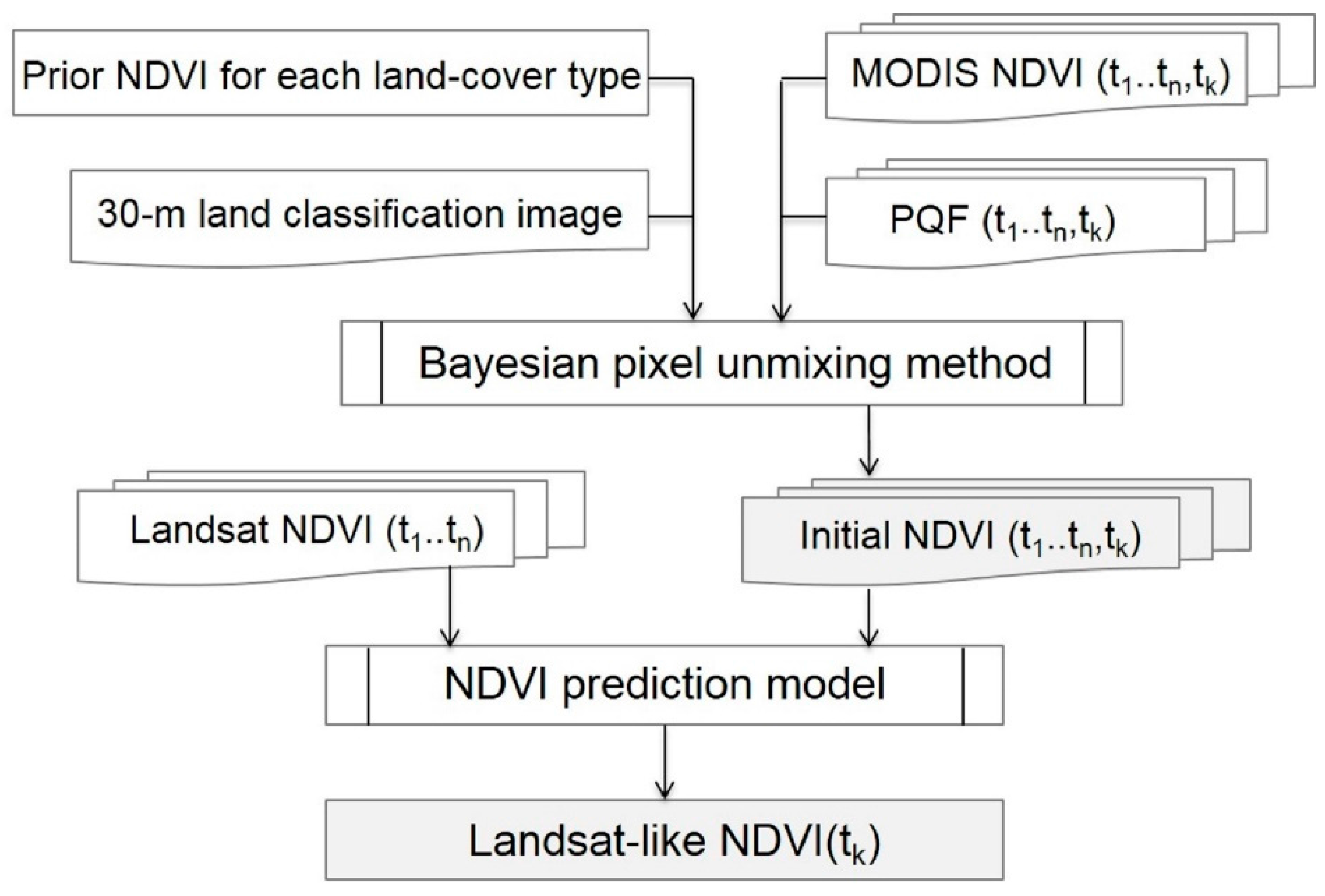
Using the 30-m resolution land classification image, the NDVI-BSFM first employed the prior MODIS NDVI datasets, the MODIS NDVI (on the paired dates $t_1$…$t_n$ and the prediction date $t_k$, i.e., $t_1$…$t_n$, $t_k$) calculated from the MOD09A1 reflectance, as well as the PQF ($t_1$...$t_n$, $t_k$), to obtain the initial NDVI ($t_1$...$t_n$, $t_k$) at 30-m resolution. This step was performed by the Bayesian pixel unmixing process, which blends the information of the prior MODIS NDVI into the traditional unmixing process. For example, the output initial NDVI on DOY = 206 in 2014 is a combination of the prior MODIS NDVI on DOY = 206 (calculated from 2008 to 2014) and the MODIS NDVI on DOY = 206 in 2014. It has the same spatial resolution as the Landsat image, but its spectral features are MODIS-like. Subsequently, an NDVI rebuilding model was applied to combine the initial NDVI ($t_1$...$t_n$, $t_k$) and Landsat NDVI ($t_1$...$t_n$) observations to predict the Landsat-like NDVI on the prediction date $t_k$. 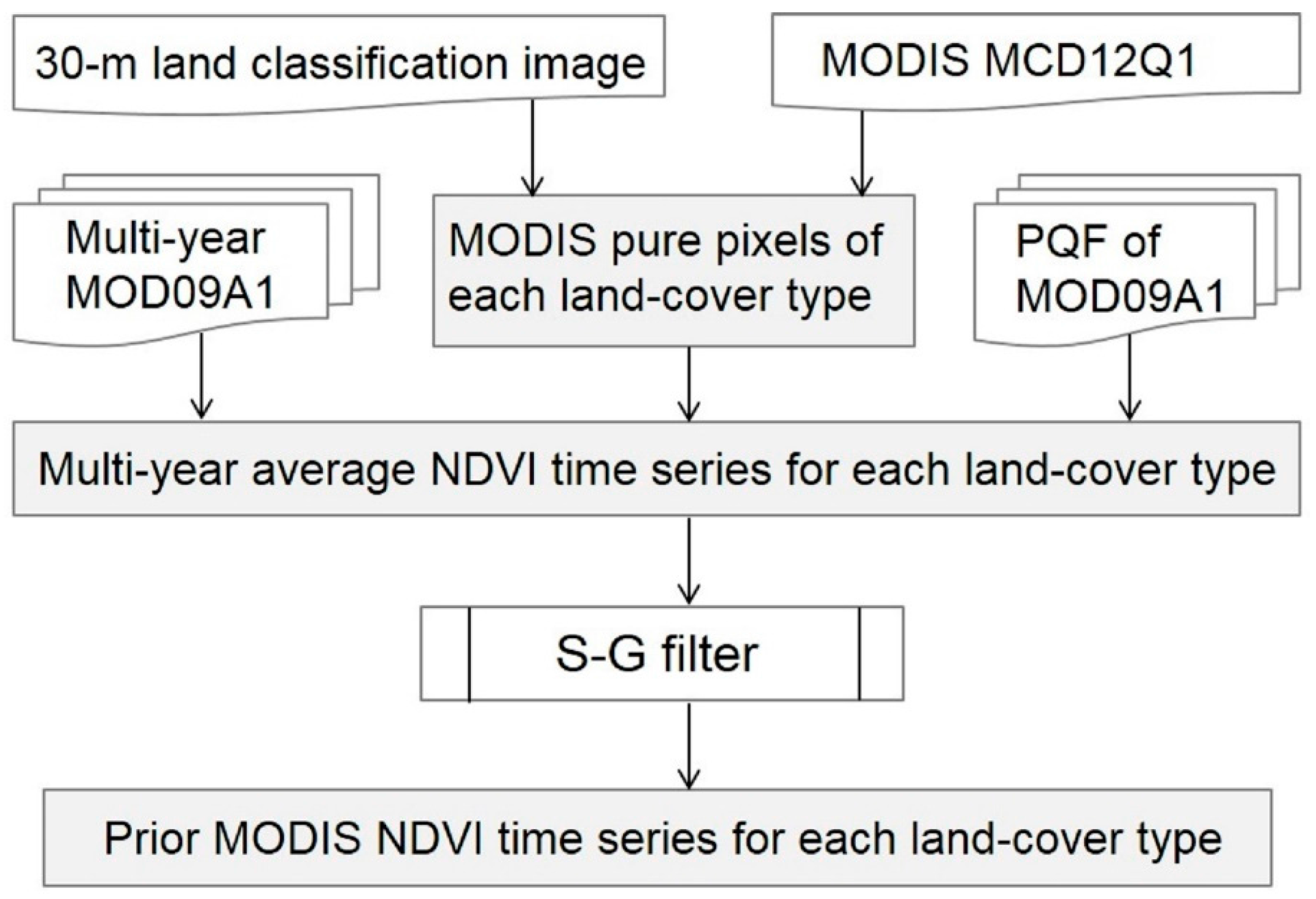Figure 4 shows a flowchart that illustrates the proposed method, and the main steps of the implementation are described in detail in the following sections.

3.1. Bayesian Pixel Unmixing Method

Unmixing-based algorithms are among the most commonly used methods for generating high spatial resolution images from coarse-resolution images based on high spatial resolution land cover classification images. Busetto et al. proposed a Weighted Linear Mixing model for downscaling MODIS NDVI, which assumes that the NDVI value of a coarse pixel can be calculated as the area fraction weighted average of the NDVI values for several land-cover endmembers at a fine spatial scale within the coarse pixel [27,28]. If there are $i$ land-cover endmembers within a MODIS pixel, then at least $i$equations should be available to avoid the inversion of ill-posed matrices. It is reasonable to employ spatially neighboring coarse pixels to provide extra information because the same land-cover endmember with a similar vegetation type in a small area can be assumed to share a similar NDVI value at a specific time according to Tobler’s First Law of Geography [39]. In general, a sliding window of (n × n) MODIS pixels is applied, where n² must equal the number of classes i or be larger than i. Thus, the neighboring pixels within the sliding window can be used to obtain a linear model, and unmixing is performed by solving the linear mixing model described by Equation (2).

$${\text{NDVI}}_{coarse}=\mathrm{A}NDV{I}_e+\mathsf{\epsilon }$$

(2)

In Equation (2), ${\text{NDVI}}_{coarse}$ is an (n² × 1) column vector containing the NDVI of each MODIS pixel in the n × n moving window that is currently being unmixed. The endmember fraction matrix A is an (n² × i) matrix, which is calculated from the 30-m resolution classification image, and $NDV{I}_e$ is an (i × 1) column vector that contains the NDVI of each land-cover types at Landsat scale, where the aim of Equation (2) is to obtain $NDV{I}_e$ by minimizing the residuals ($\mathsf{\epsilon }$) introduced by the linear mixing model.

However, it is known that unmixing may yield unrealistic estimates of the endmember values, and several studies have aimed to address this problem [9,29,40]. In addition, it should be considered that the decomposition results are totally dependent on the quality of the coarse-resolution image, so decomposition based on a coarse-resolution image that contains large amounts of noise would never get the correct results. Therefore, there is still room for improving the accuracy of traditional decomposition strategies. In this study, we employed a Bayesian theory based solution, which is based mainly on a previous method [9], to constrain the estimation of the endmembers.

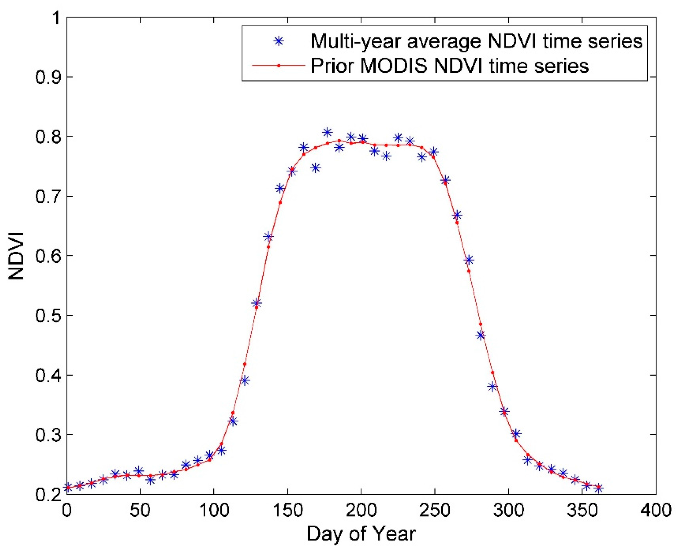
We treated the filtered multi-year average NDVI time series of pure MODIS pixels for each land-cover type as prior information, where this process is described in Section 2.2. Furthermore, we assumed a Gaussian distribution for the prior probability with mean $NDV{I}_p$ and covariance matrix ${\mathsf{\Sigma }}_p$. We also assumed that the MODIS NDVI observations ($NDV{I}_o$) were noisy within the sliding widow, where they followed a Gaussian distribution with covariance matrix ${\mathsf{\Sigma }}_o$. In these conditions, the posterior distribution follows a Gaussian distribution with expectation value ${\mathsf{\mu }}_e$ and covariance matrix ${\mathsf{\Sigma }}_e$. Finally, the following expressions can be obtained according to Bayes’ theorem of conditional probabilities [41]:

$${\mathsf{\Sigma }}_e={[{\mathsf{\Sigma }}_p^{-1}+A^T{\mathsf{\Sigma }}_o^{-1}A]}^{-1}$$

(3)

$${\mathsf{\mu }}_e={\mathsf{\Sigma }}_e\left[A^T{\mathsf{\Sigma }}_o^{-1}NDV{I}_o+{\mathsf{\Sigma }}_p^{-1}NDV{I}_p\right]$$

(4)

Note that ${\mathsf{\mu }}_e$ is the expectation value for the posterior probability, which is also the minimum mean squared estimator of the endmembers. According to the equations given above, we can conclude that the expectation value for the endmembers comes from a combination of prior knowledge and the MODIS NDVI observations.

It is important to define the covariance matrices, so we employed spherical covariance matrices, as described in a previous study [9], to define ${\mathsf{\Sigma }}_p$ and ${\mathsf{\Sigma }}_o$ as follows:

$${\mathsf{\Sigma }}_p={\mathsf{\sigma }}_p^{2}I\left(i\right)$$

(5)

$${\mathsf{\Sigma }}_o={\mathsf{\sigma }}_o^{2}I\left(n^2\right)$$

(6)

where I(i) and I(n²) represent the (i × i) and (n² × n²) identity matrices, respectively, and ${\mathsf{\sigma }}_p^2$ and ${\mathsf{\sigma }}_o^2$ represent the variances assigned to the prior $NDV{I}_p$ and the observation $NDV{I}_o$, respectively. The individual values of ${\mathsf{\sigma }}_p^2$ and ${\mathsf{\sigma }}_{\mathrm{o}}^2$ are not remarkable, but the ratio ${\mathsf{\sigma }}_{ratio}={\mathsf{\sigma }}_p/{\mathsf{\sigma }}_o$ is the key index for controlling the relative importance of the prior information and the observations. If the observations are of poor quality according to the PQF, then after reducing the ${\mathsf{\sigma }}_{ratio}$, more stress is placed on the prior information, thereby decreasing the influence of the observation noise on the estimators, and vice versa. Therefore, better results can be obtained by optimizing${\mathsf{\sigma }}_{ratio}$.

It should be noted that, the fixed window is moved pixel by pixel, so the equations and results obtained differ from the MODIS pixels. Following the steps described above, each MODIS pixel yielded a set of expected NDVI values for the posterior probability for each class. Finally, the pixels at Landsat scale within a MODIS pixel were assigned the corresponding class’s expected NDVI value, which we refer to as the so-called “initial NDVI” in the next section, according to the 30-m resolution classification image.

3.2. High Spatial and Temporal NDVI Rebuilding Model

The initial NDVI images at Landsat resolution synthesized from the MODIS data, as described in the previous section, were not Landsat-like images, but instead they were MODIS-like images. For one thing, the spectral features of the initial NDVI images were inherited from MODIS. For another thing, the initial NDVI images contained no spatial details similar to those in Landsat images. Moreover, in the initial NDVI images, the within-class variations in a MODIS pixel were totally ignored. In order to build Landsat-like NDVI images, the relationships between observations of real Landsat NDVI images acquired on the paired dates and their corresponding initial NDVI were required in a rebuilding model to adjust the initial NDVI on the prediction date to Landsat-like NDVI, this step was done pixel by pixel.

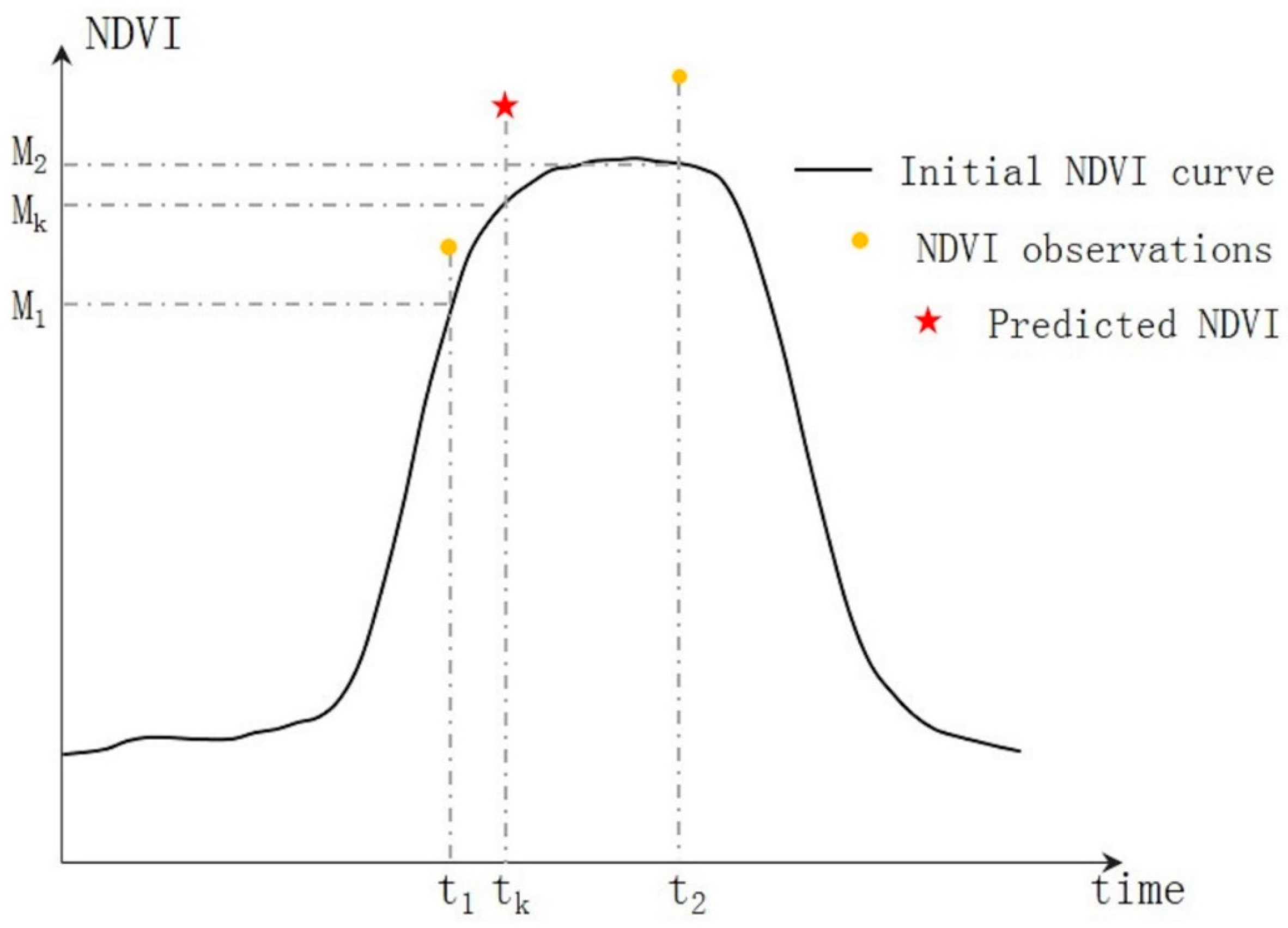
We assumed that the initial NDVI growth of a vegetation pixel followed a pattern, such as the one shown in Figure 5. Mainly due to the sensor differences and other uncertainties, the relationship between the NDVI derived from Landsat data (L_t) and the initial NDVI calculated from MODIS data ($M_t$) on date t can be expressed as follows.

$$L_t=M_t+{\mathsf{\epsilon }}_t$$

(7)

In Equation (7), the difference term ${\mathsf{\epsilon }}_t$, which was regarded as a constant in most previous studies [13,14], would actually change over time duo to phenology. For example, it is reasonable for the difference term ${\mathsf{\epsilon }}_t$ to equal 0.2 in summer when the vegetation is at its most luxuriant, whereas it would impossible for it to reach 0.2 in winter when the plants are withered and the NDVI is close to 0. If we assume two distinguishable dates $t_1$ and $t_k$, then the relationship between the Landsat NDVI and the initial NDVI on the two dates can be accordingly expressed by Equations (8) and (9), respectively.

$$L_1=M_1+{\mathsf{\epsilon }}_1$$

(8)

$$L_k=M_k+{\mathsf{\epsilon }}_k$$

(9)

In general, the initial NDVI, which is downscaled from MODIS NDVI, can represent the vegetation status and the range of ${\mathsf{\epsilon }}_t$ will be larger when the initial NDVI ($M_t$) is higher. Hence, we assumed a positive correlation between ${\mathsf{\epsilon }}_t$ and $M_t$. Combining Equations (8) and (9), the relationship between $L_1$ and $M_1$ on date $t_1$ and $L_k$ and $M_k$ on date $t_k$ can be described as follows.

$$\frac{L_1-M_1}{M_1}=\frac{L_k-M_k}{M_k}$$

(10)

If we take the predicted Landsat NDVI $L_k$ as the variable that needs to be solved, then Equation (10) can be translated into the following form.

$$L_k=M_k+\frac{M_k\times \left(L_1-M_1\right)}{M_1}$$

(11)

Thus, if we determine the initial NDVI and the Landsat NDVI for the pair on date t₁, and the initial NDVI on date t_k in advance, then we can obtain the Landsat NDVI on date t_k by applying Equation (11). In addition, from Equation (11), we can find that the predicted Landsat NDVI is based on the initial NDVI on the prediction date, as well as being adjusted by the relationship between the initial NDVI and Landsat NDVI paired on another date. However, an adjustment that relies on only one pair of images is not always valid and the real situation is complicated by several factors, including the intricate dynamics of vegetation growth, changes in the land-cover type, atmospheric impacts, and various other factors. If more than one Landsat images within a region can be acquired during one year, the extra information with multiple temporal phases can be highly beneficial, thereby contributing to more reliable results. Equation (12) provides a method for combining n pairs of initial NDVI and Landsat NDVI on dates from $t_1$ to $t_n$ to predict the Landsat NDVI on date $t_k$:

$$L_k=M_k+\frac{{{\displaystyle \sum }}_{j=1}^n\mathsf{\omega }\left(t_k,t_j\right)\times \frac{M_k\times \left(L_j-M_j\right)}{M_j}}{{{\displaystyle \sum }}_{j=1}^n\mathsf{\omega }\left(t_k,t_j\right)}$$

(12)

where j is a variable that ranges from 1 to n, $L_j and M_j$ are the Landsat NDVI and the initial NDVI on date $t_j$, respectively, and the weight $\mathsf{\omega }(t_k,t_j$) determines the contribution of the NDVI pair on date $t_j$ to the adjustment.

To define the weight $\mathsf{\omega }(t_k,t_j$), two features need to be considered. First, paired data on closer dates can provide a more accurate indication of the estimator because plants grow gradually. Second, paired data for which the initial NDVI has a greater correlation coefficient with respect to the initial NDVI on the prediction date can be more representative of the status of the NDVI on the prediction date. To consider both features, the weighting factor $\mathsf{\omega }(t_k,t_j$) was defined as follows.

$$\mathsf{\omega }\left(t_k,t_j\right)=\frac{1}{t_k-t_j}\times \frac{1}{M_k-M_j}$$

(13)

In Figure 5, $t_1$ is nearer to $t_k$, and $M_2$ is closer to $M_k$, so the paired data on dates $t_1$ and $t_2$ both play important roles in adjusting the estimator on date $t_k$.

In conclusion, the proposed model first uses a Bayesian based method to introduce the prior MODIS NDVI into the unmixing process to yield a more accurate initial NDVI at the Landsat scale, before combining the initial NDVI and Landsat NDVI image pairs acquired on other dates to rebuild the Landsat-like NDVI on prediction date. This model can predict a single Landsat-like NDVI image as well as building a Landsat-like NDVI time-series dataset.

4. Experiments and Results

In this research, experiments over two study areas were conducted. On the one hand, a small area in Huailai, Hebei Province, China, was used to demonstrate the performance from different aspects by comparison with STARFM and ESTARFM predictions. On the other hand, a Landsat tile in Yunnan Province, China, was also used to test the effectiveness of the proposed method when applied to large areas.

The parameter ${\mathsf{\sigma }}_{ratio}$ was demonstrated to significantly reduce the prediction errors when equal variance was assigned to prior information and measurements (${\mathsf{\sigma }}_{ratio}$ = 1) compared with an almost unconstrained estimate in a previous study [9]. In the present study, we optimized the ${\mathsf{\sigma }}_{ratio}$ to obtain better results, which we set to 0.5 when the MODIS NDVI measurements had ideal quality and 4 for poor quality empirically, according to the MODIS PQF. Hence, if the MODIS NDVI measurements that needed to be unmixed had ideal quality, more importance was placed on the MODIS NDVI measurements, whereas if the MODIS NDVI measurements were noisy signals, they had to be highly restricted by the prior information, therefore more importance was placed on the prior information.

We also conducted evaluations and different comparisons to comprehensively confirm the robustness of the proposed method. We calculated four statistics between the predictions and the Landsat observations to quantify the global accuracy, i.e., the Average Absolute Difference ($\text{AAD}$, Equation (14)), the Average Absolute Relative Difference ($\text{AARD}$, Equation (15)), the correlation coefficient ($r$, Equation (16)), and the Root Mean Square Error ($\text{RMSE}$, Equation (17)), as follows:

$$\text{AAD}=\frac{1}{n}{{\displaystyle \sum }}_{i=1}^n|NDV{I}_i^p-NDV{I}_i^o|$$

(14)

$$\text{AARD}=\frac{1}{n}{{\displaystyle \sum }}_{i=1}^n|(NDV{I}_i^p-NDV{I}_i^o)/NDV{I}_i^o|$$

(15)

$$r=\frac{{\displaystyle {\sum }_{i=1}^n\left(NDV{I}_i^p-\overline{NDV{I}^p}\right)\left(NDV{I}_i^o-\overline{NDV{I}^o}\right)}}{\sqrt{{\displaystyle {\sum }_{i=1}^n{\left(NDV{I}_i^p-\overline{NDV{I}^p}\right)}^2}}\cdot \sqrt{{\displaystyle {\sum }_{i=1}^n{\left(NDV{I}_i^o-\overline{NDV{I}^o}\right)}^2}}}$$

(16)

$$\text{RMSE}=\sqrt{\frac{{{\displaystyle \sum }}_{i=1}^n{\left(NDV{I}_i^p-NDV{I}_i^o\right)}^2}{n}}$$

(17)

where $NDV{I}_i^p$ and $NDV{I}_i^o$ are the predicted and observed values for pixel i, respectively.

4.1. Performance Comparison over a Small Region

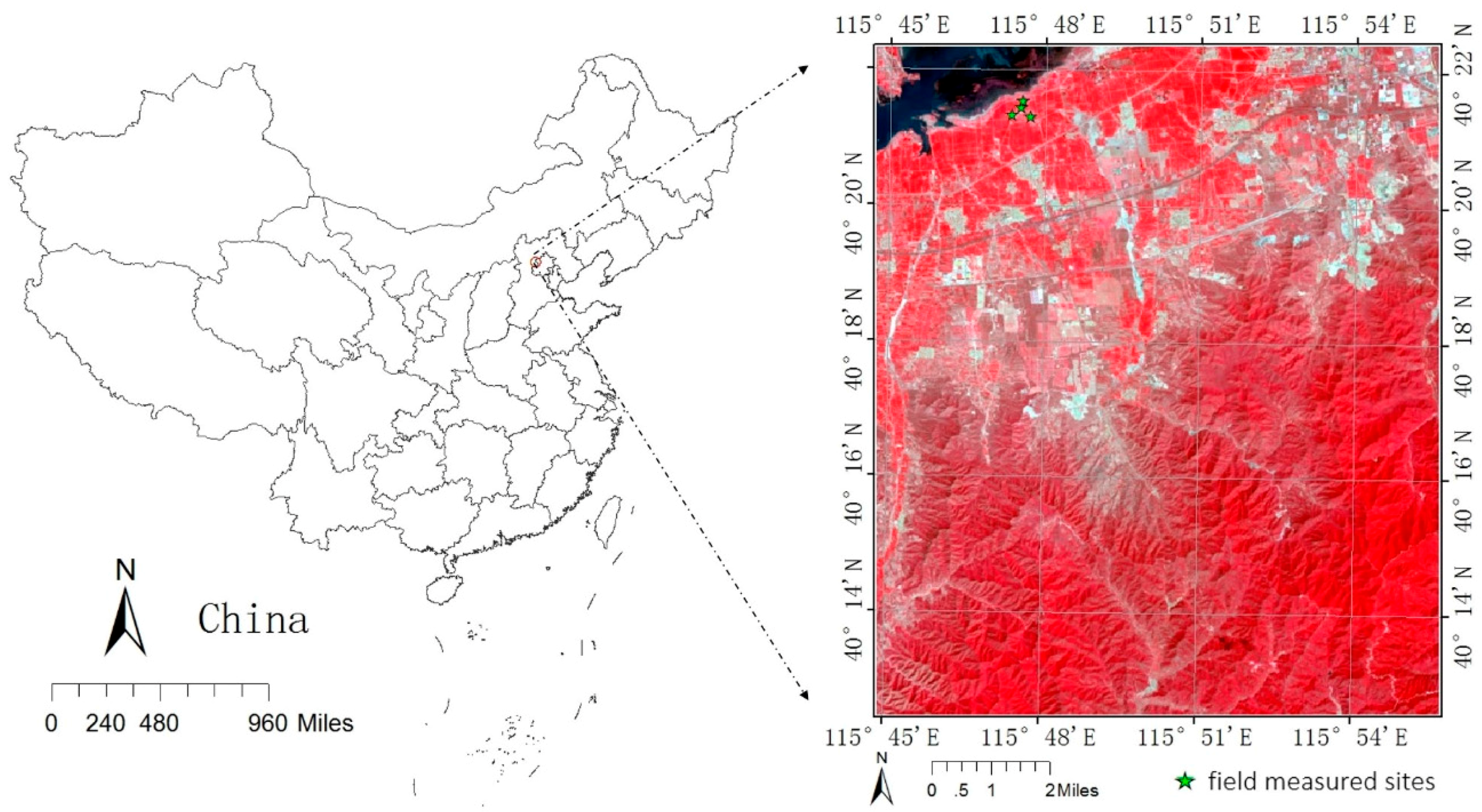
4.1.1. Study Area of Huailai

The Huailai area is located around the experimental station of the Institute of Remote Sensing and Digital Earth, Chinese Academy of Sciences (40°21′ N, 115°47′ E) in Huailai County, Hebei Province, China. The site consists of a rectangular area of 280 km², which corresponds to 608 × 512 Landsat pixels. The typical elevation of the site is about 480 m and it has a temperate continental climate. The study area is mainly made up of forests, farmland predominantly planted with corn, and shrubland. Figure 6 shows the location and survey of the Huailai area.

The Huailai area was covered by two Landsat scenes (WRS-2 path 123 and row 32, path 124 and row 32), so there was a high probability of obtaining cloud-free Landsat images. In fact, we obtained 14 cloud-free Landsat 8 surface reflectance imageries (DOY = 14, 30, 94, 119, 142, 206, 222, 238, 247, 270, 279, 286, 318, and 359) in 2014, ensuring abundant validation data for the proposed approach. Furthermore, field experiments were performed at this site throughout 2014, when in-situ NDVI datasets were collected. The availability of suitable data motivated the selection of the Huailai site as a study area.

In this part of the work, a total of three Landsat and MODIS image pairs of the Huailai area from 2014 (DOY = 94, 206, and 286), as shown in Figure 7, were used as input datasets. Among them, only two image pairs (DOY = 94 and 206) were used in Section 4.1.2 to retrieve single Landsat-like NDVI images. In the work described in Section 4.1.3, the three image pairs were all used to build Landsat-like NDVI images for all of 2014.

4.1.2. Retrieving Single Landsat-Like NDVI Images

In general, the MODIS NDVI on the date upon which the predicted Landsat-like NDVI is based has a crucial impact on the predicted result. In this section, we describe the performance of the proposed method using both ideal and poor quality MODIS NDVI data on the prediction date. As noted, two input NDVI image pairs on DOY = 94 and 206 were used in the work described in this section.

First, we tested the NDVI-BSFM in an ideal situation, where the MODIS NDVI image on the prediction date was of ideal quality, to retrieve a Landsat-like NDVI image on the date DOY = 238. In addition, STARFM and ESTARFM were used to obtain the NDVI for comparison by indirectly predicting the red and NIR bands using the same input datasets.

Figure 8 shows that the three methods all produced excellent results. However, NDVI-BSFM yielded more realistic and detailed spatial information compared with STARFM, because the neighboring pixels were used to obtain a weighted average prediction of the center pixel in STARFM, which produces more reliable predictions but it also loses small spatial characteristics to give a hazy appearance. In contrast, NDVI-BSFM does not consider the neighborhood information during the prediction step and it is based only on the predicted pixel itself, thereby preserving its specific characteristics. In this experiment, ESTARFM successfully preserved spatial details, thereby demonstrating its advantage compared with STARFM.

The overall accuracy of NDVI-BSFM was higher than that of STARFM and ESTARFM according to the global assessment indices shown in

Table 1. AAD, AARD, r and RMSE between the predicted NDVI values obtained using the three methods and actual Landsat NDVI observations on DOY = 238.

Method	AAD	AARD	r	RMSE
STARFM	0.0574	15.42%	0.9144	0.0904
ESTARFM	0.0469	12.31%	0.9342	0.0802
NDVI-BSFM	0.0459	11.85%	0.9663	0.0648

. The values of AAD, AARD, and RMSE for the predictions obtained using NDVI-BSFM were lower than those for the predictions made using STARFM and ESTARFM. The correlation coefficient ($r$) for NDVI-BSFM was 0.9663, which was much higher than that for STARFM and ESTARFM, i.e., 0.9144 and 0.9342, respectively, thereby indicating better agreement with the actual Landsat NDVI values calculated directly from the Landsat 8/OLI reflectance image acquired on the prediction date.

The errors in the predicted NDVI obtained using NDVI-BSFM had several causes. First, the eight-day composite cycle of MOD09A1 made the MODIS NDVI more reliable, but it also led to mismatches and further increasing the uncertainty of the relationship between the paired initial NDVI and Landsat NDVI data. Second, uncertainties in the Landsat and MODIS datasets, errors in the 30-m resolution land cover map, and surface disturbances that occurred over the paired and prediction dates all introduced deviation into the final estimators.

For most downscaling strategies, including STARFM, the effects of noisy signals in paired images can be reduced in an effective manner by a weighted mechanism, but the quality of the coarse-resolution data on the prediction date, from which the predicted results are mainly inherited, is a fatal constraint on prediction accuracy. In fact, even the eight-day composited MODIS MOD09A1 datasets, which have better data quality than MODIS daily reflectance products, still inevitably contain bad pixels. If the bad pixels were joined into patches or blocks, local estimators could never eliminate these effects. In this study, bad pixels were detected by the MODIS PQF and corrected using prior information by applying a Bayesian framework. Therefore, in theory, the proposed method was expected to perform well routinely, regardless of the MODIS NDVI data quality.

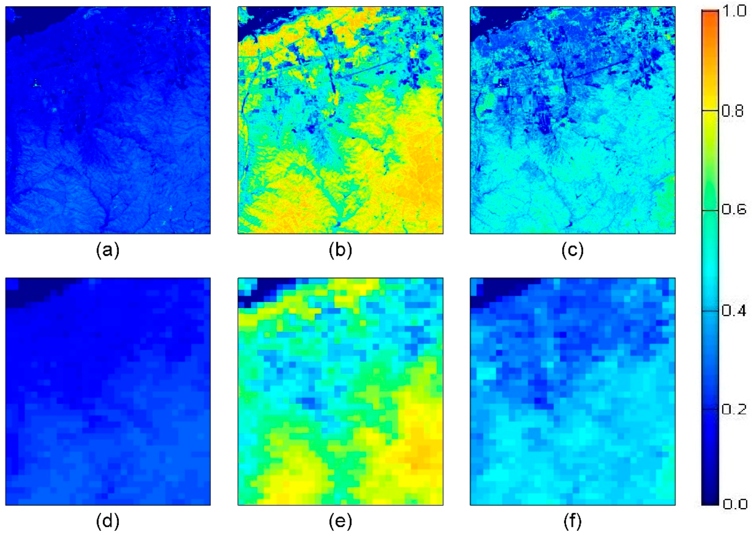
Within the Huailai area, the MODIS NDVI image on DOY = 217 was of poor quality, and hence experiments was conducted to retrieve the Landsat-like NDVI image on DOY = 217 in this case. Figure 9 and

Table 2. Values of AAD, AARD, r and RMSE between the predicted NDVI values produced using the two methods and the actual Landsat NDVI observations on DOY = 217.

Method	AAD	AARD	r	RMSE
STARFM	0.1184	24.79%	0.7830	0.1535
ESTARFM	0.1435	29.89%	0.7306	0.1899
NDVI-BSFM	0.0544	13.62%	0.9457	0.0706

show that STARFM was incapable of capturing the spatial details and barely reflected the ground truth, and ESTARFM yield incorrect spatial characteristics, that were deeply affected by the MODIS bad pixels on DOY = 217. In contrast, NDVI-BSFM successfully built realistic NDVI estimators, which were highly correlated with the real Landsat NDVI image. The values of AAD, AARD, and RMSE for NDVI-BSFM were less than half those for STARFM and ESTARFM, but $r$ remained at a high level of 0.9457, thereby demonstrating that NDVI-BSFM could routinely perform better than STARFM with very poor-quality MODIS data on the prediction dates. Nevertheless, NDVI-BSFM over-estimated the results at the lower right part of the image because of the abnormally high values in MODIS NDVI, which were omitted by MODIS PQF.

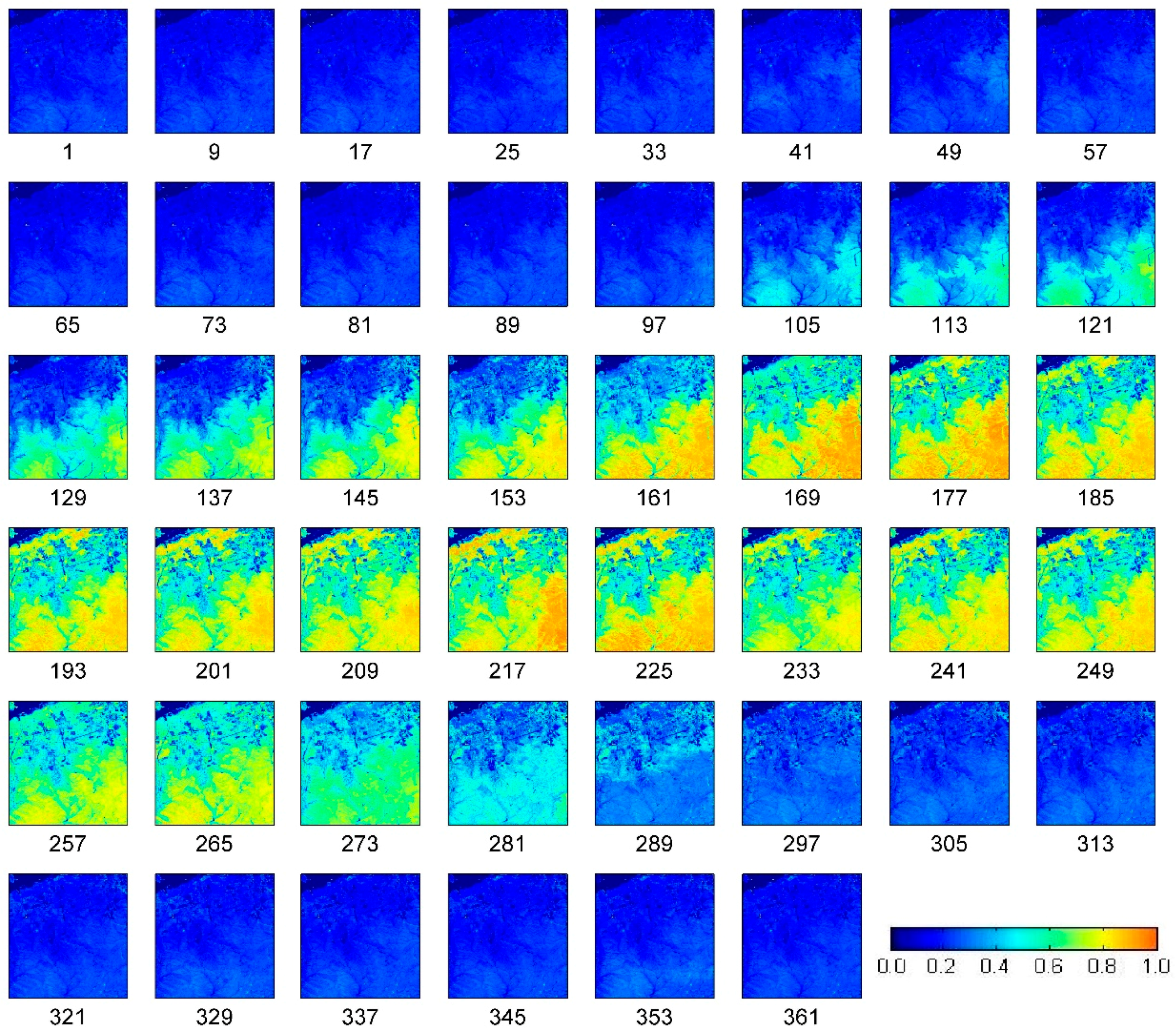
4.1.3. Retrieving Landsat-Like NDVI Time Series

During the development of NDVI-BSFM to retrieve Landsat-like NDVI time series, we aimed to address two main issues. First, the accuracy of NDVI-BSFM was tested repeatedly with different inputs, thereby allowing the general performance of NDVI-BSFM to be summarized. Second, building high-quality Landsat-like NDVI time series was an important goal of this study, because high spatial resolution NDVI datasets with frequent coverage are required to extract and separate information on vegetation change due to phenological cycles, inter-annual climatic variability, and long-term trends [24]. In this study, in addition to predicting single NDVI images, as described in Section 4.1.2, we retrieved all the eight-day Landsat-like NDVI images throughout 2014 using the same three paired NDVI images. Figure 10 shows that the phenology of the vegetation was clearly visible, where the NDVI of the vegetation region within the study area started to increase in the spring before peaking during the summer and then declining in the winter. Nevertheless, discontinuities were also visible in the predicted NDVI time series. These were basically inherited from the corresponding MODIS NDVI images and were mainly due to cloud contamination, errors in the atmospheric correction process and angle effects.

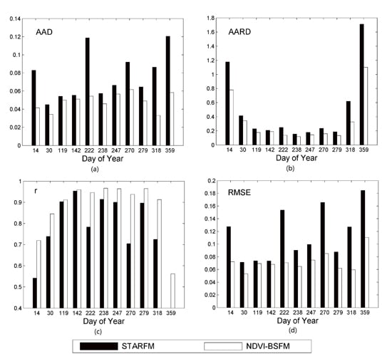
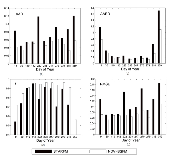
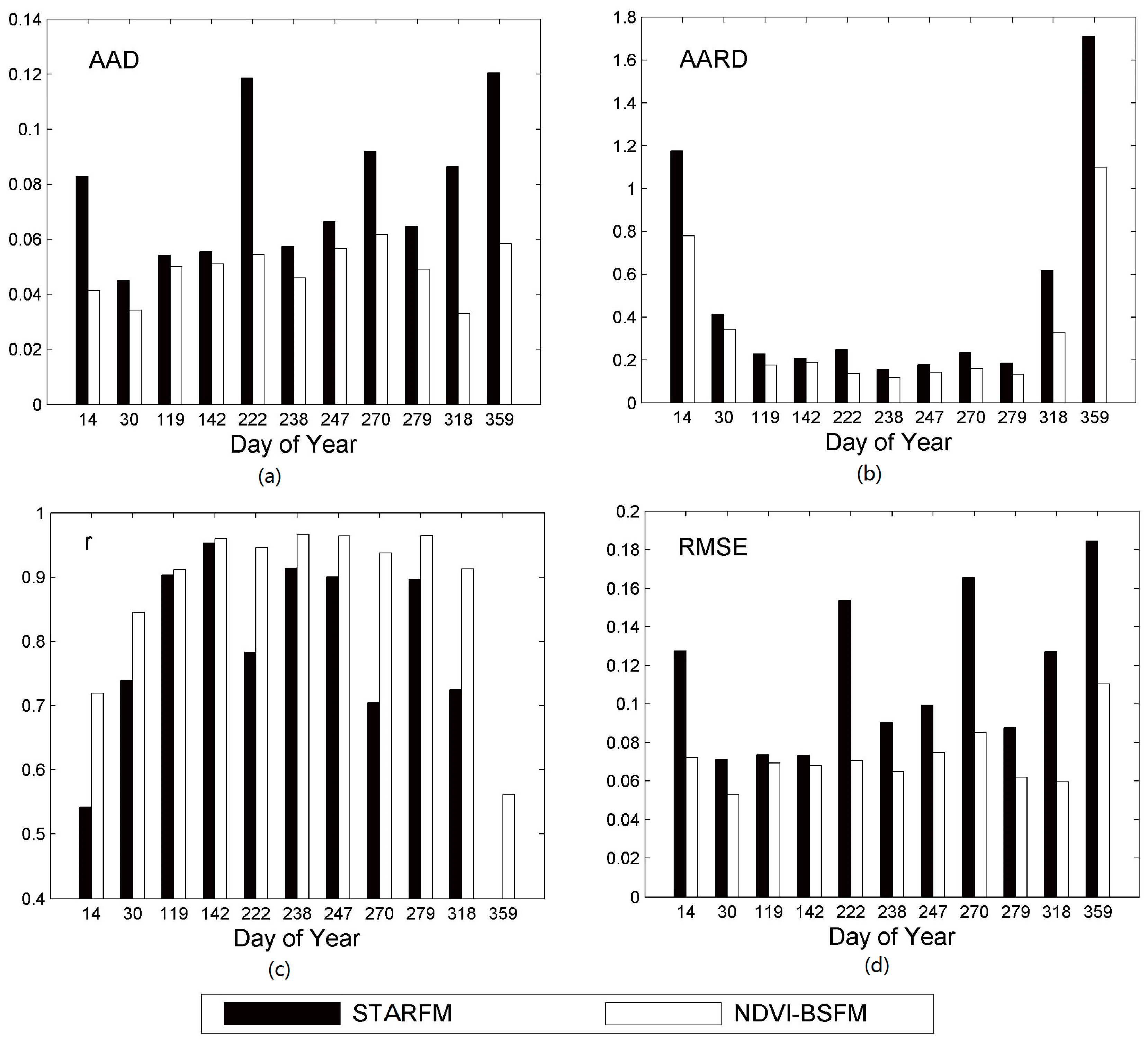
We employed the AAD, AARD, $r$, and RMSE indices to quantitatively evaluate the accuracy of the estimators. When excluding the three paired Landsat acquisitions, the remaining 11 Landsat observations of the 14 cloud-free Landsat images acquired during 2014 were used as the true values to check the performance of the method. As shown in Figure 11, for each prediction, the values of AAD, AARD, and RMSE obtained using NDVI-BSFM were stably and considerably lower than those produced with STARFM, and the value of $r$ was persistently higher using NDVI-BSFM. In addition,

Table 3. Comparison of the average accuracy assessments by the two methods for each prediction.

Methods	Average AAD	Average AARD	Average r	Average RMSE
STARFM	0.0767	48.66%	0.7685	0.1140
NDVI-BSFM	0.0487	32.78%	0.8808	0.0718

shows the average assessments for the 11 evaluations, where the average values of AAD, AARD, $r$, and RMSE (0.0487, 0.3278, 0.8808, and 0.0718, respectively) were excellent for NDVI-BSFM. Overall, we can conclude that NDVI-BSFM obtained superior performance compared with STARFM, and hence it is a powerful new approach for the construction of NDVI time series.

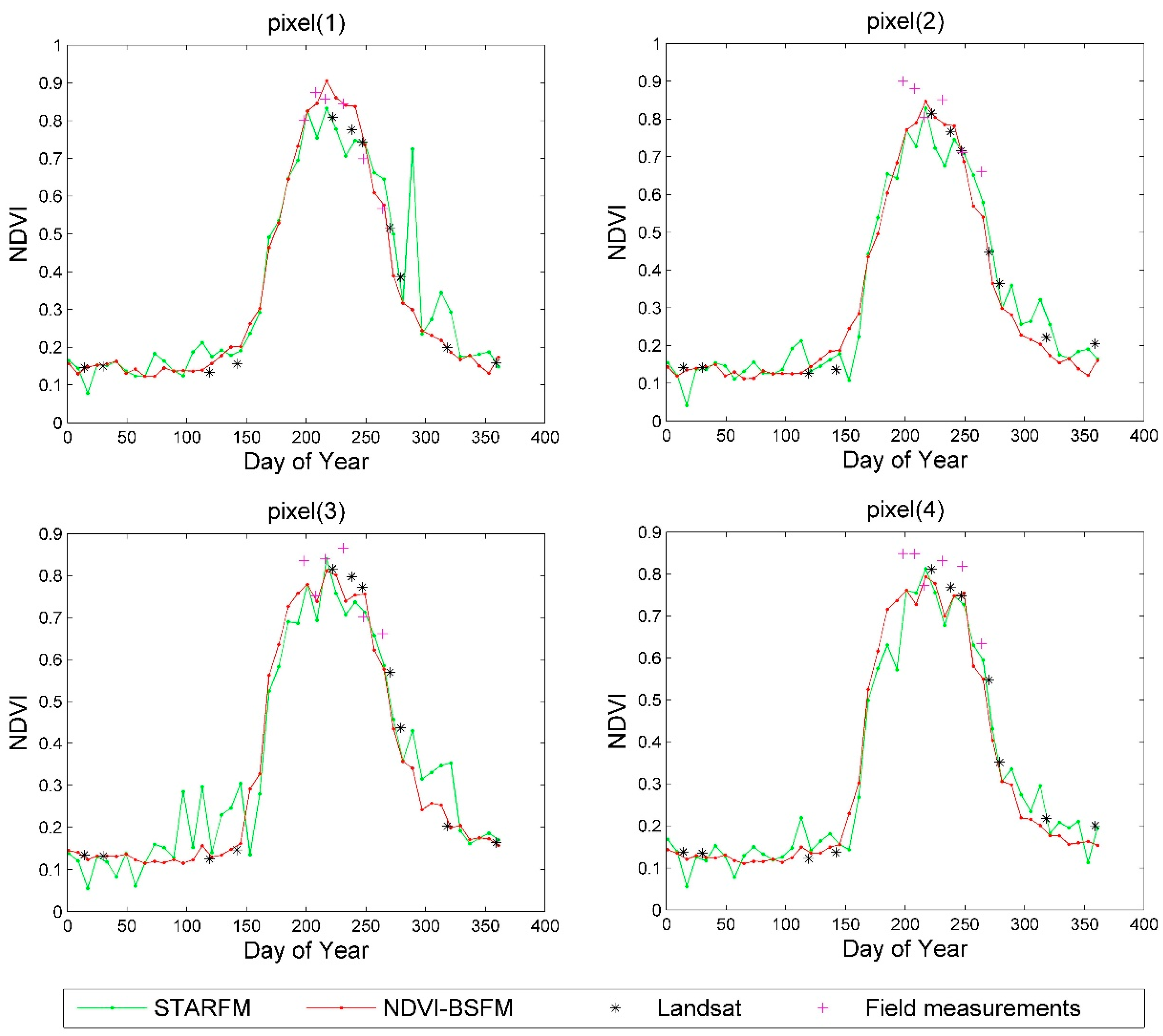
In addition, during 2014, experiments were performed to collect the spectrum reflectance at several locations in the study area using the SVC HR-1024 field spectroradiometer. Next, the reflectances of the red and NIR bands, which were employed to calculate the measured NDVI directly, were generated using the Landsat 8/OLI spectral response function. Finally, the field measurements of some pixels and their corresponding Landsat 8/OLI observations were utilized as reference values to assess the temporal NDVI profiles. Thus, NDVI time series profiles of four vegetated pixels with field measurements produced by NDVI-BSFM and by STARFM were both compared with the references, and the results are shown in Figure 12.

According to Figure 12, the NDVI time series curves produced by NDVI-BSFM were closer to the references than those produced by STARFM, thereby demonstrating the greater accuracy and suitability of the proposed method. In particular, the field measurements were comparatively higher, which was mostly due to scale effects because the experiments were fixed at points, whereas the Landsat pixels were made up of polygons with a spatial extent of 30 m, thereby causing some unavoidable disagreements. In addition, the major fluctuations in STARFM NDVI curves were mainly due to accumulated errors when predicting the reflectance of the red and NIR bands, whereas the regularities in the NDVI time series for a vegetation pixel should increase and decrease gradually. In contrast, the NDVI time series profiles produced by NDVI-BSFM were smoother, thereby demonstrating that NDVI-BSFM is more effective in retrieving NDVI time series.

4.2. Application over a Large Area

Note that the Huailai test site may be too small to draw comprehensive and credible conclusions from the comparison. In addition, obtaining several cloud-free Landsat observations within a year in some humid areas is usually difficult, and therefore it is sometimes necessary to predict with only one input image pair. Among the existing methods, STARFM is regarded as able to predict with only one input image pair, but ESTARFM was designed to work with two or more input image pairs. Recently, a new data fusion method FSDAF, was demonstrated to achieve better results with higher accuracy, more spatial details, and better retrieval of land-cover type changes with only one input image pair [23]. Therefore, for a case where only one input image pair was used, the proposed method was quantitatively compared with STARFM and FSDAF in a larger area with varying land-surface characteristics, i.e., a Landsat tile in Yunnan Province, China.

4.2.1. Study Area in Yunnan

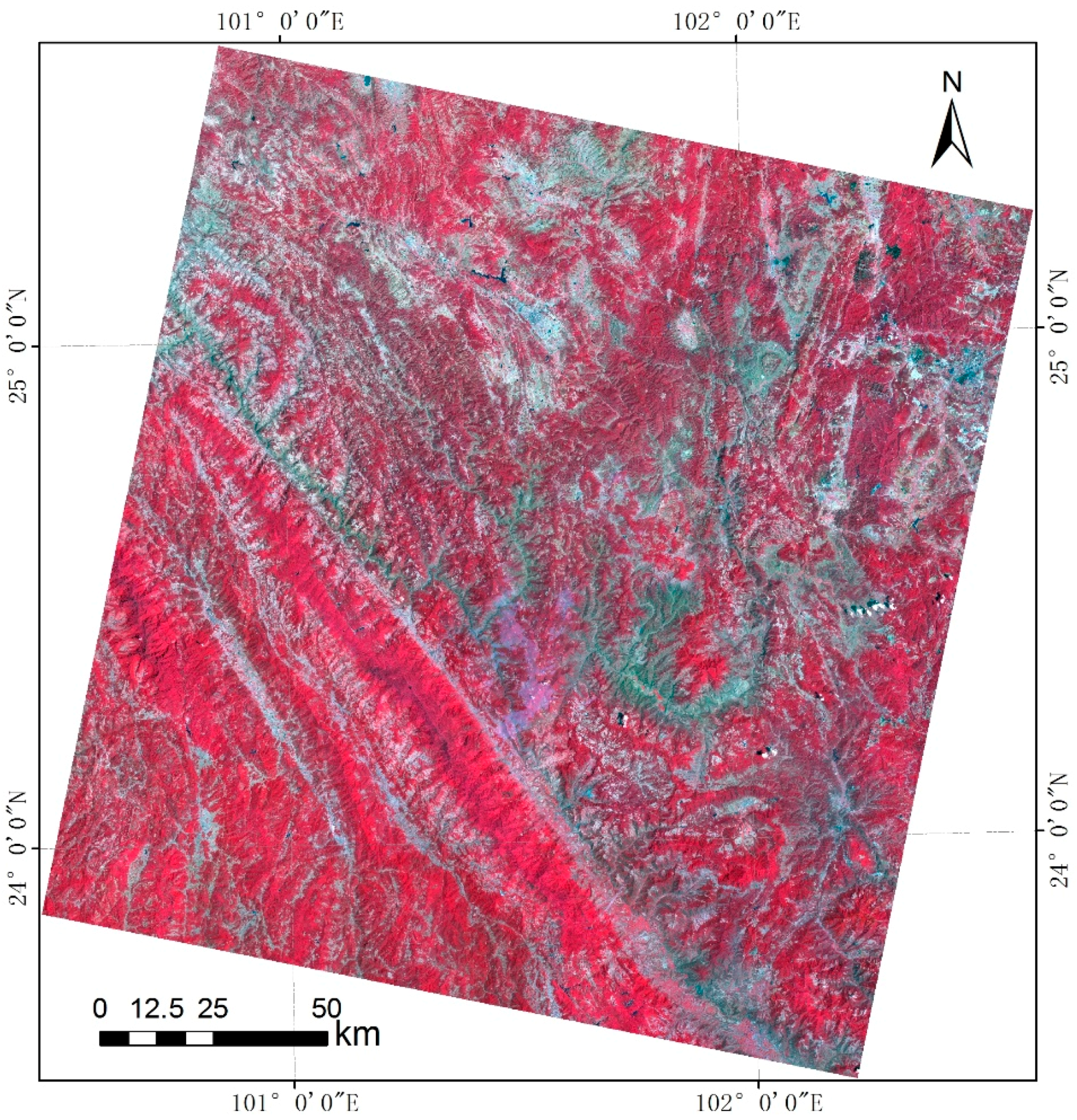
This site is a Landsat tile (WRS-2 path 130 and row 43) located in the center of Yunnan Province, China. The tile is 7278 × 7585 pixels in extent at 30-m scale, and is centered at 24°33′ N and 115°33′ E, close to the tropic of cancer. The species is rich, and multiple cropping is predominant due to the subtropical monsoon climate. The land cover in this area consists of forests, shrubland, and farmland. Figure 13 shows the location and survey of the Yunnan area.

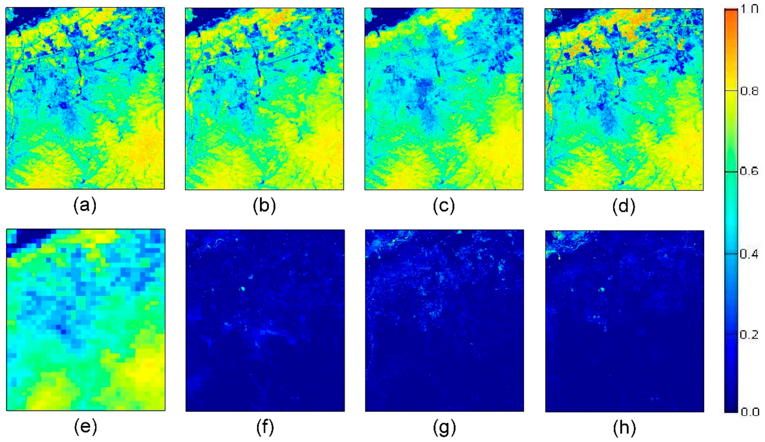
4.2.2. Retrieving NDVI Image of a Landsat Tile

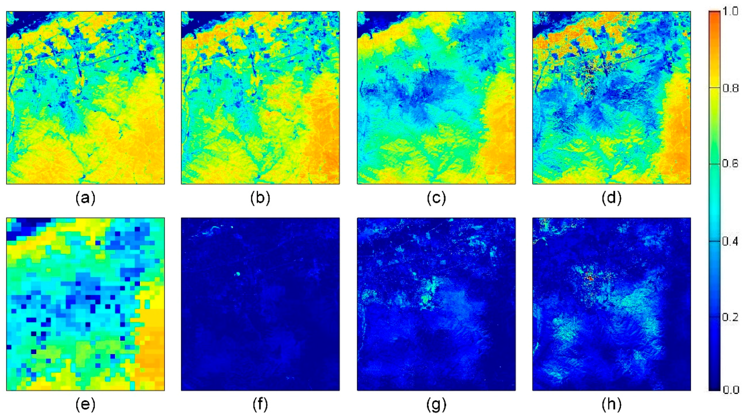
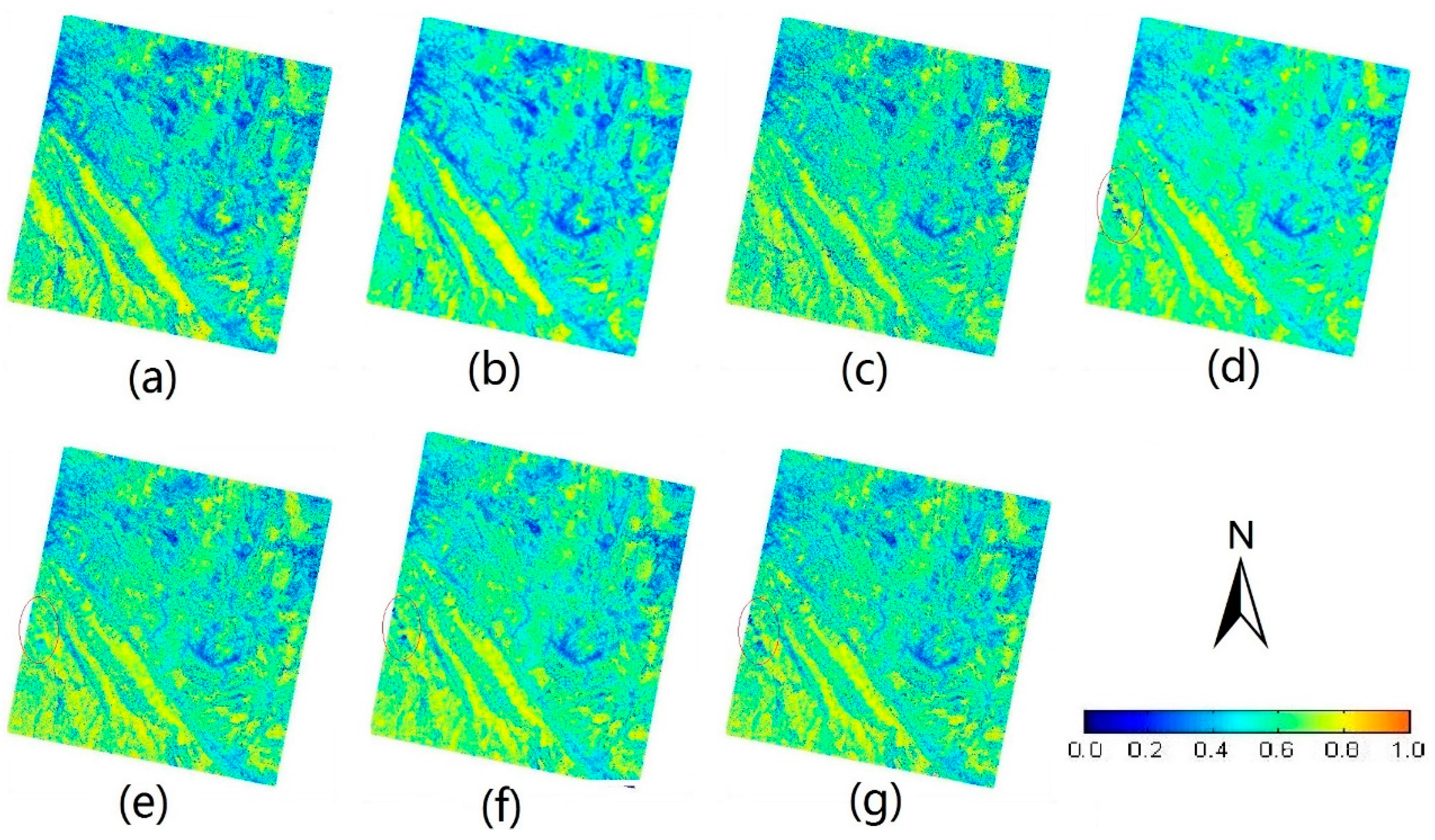
In the Yunnan area, we obtained two less cloudy Landsat 8 surface reflectance imageries (DOY = 56 and 104) in 2014. We used NDVI image pair on DOY = 104 to predict a Landsat-like NDVI image on DOY = 56, and the actual Landsat NDVI pixels with good quality (after removing bad pixels) on DOY = 56 were used as the criterion to evaluate the performance of NDVI-BSFM, STARFM and FSDAF. The results are shown in Figure 14, and the quantitative assessments are presented in

Table 4. Values of AAD, AARD, r and RMSE between the predicted NDVI values produced using the three methods and the actual Landsat NDVI observations in Yunnan area.

Methods	AAD	AARD	r	RMSE
STARFM	0.0608	13.12%	0.8461	0.0911
FSDAF	0.0582	13.21%	0.8758	0.0806
NDVI-BSFM	0.0563	12.21%	0.8847	0.0793

.

In Figure 14, NDVI images produced by NDVI-BSFM (Figure 14e), by FSDAF (Figure 14f) and by STARFM (Figure 14g) are all highly correlated with the actual Landsat NDVI image (Figure 14c). Clearly, there are larger errors in the left-hand part of the images (in the red circles) predicted by FSDAF and by STARFM. These are mainly inherited from the corresponding bad pixels in the MODIS NDVI image on the prediction date (Figure 14d). On the other hand, NDVI-BSFM worked better in this case because the bad pixels in the MODIS NDVI image were detected by the MODIS PQF and then compensated for by prior information. In fact, bad pixels in MODIS data pose a serious problem, especially in humid areas.

The comparison results shown in Table 4 determined that the three methods had comparable overall accuracy in this experiment. However, NDVI-BSFM (AAD: 0.0563, AARD: 12.21%, r: 0.8847 and RMSE: 0.0793) performed slightly better than FSDAF (AAD: 0.0582, AARD: 13.21%, r: 0.8758 and RMSE: 0.0806) and STARFM (AAD: 0.0608, AARD: 13.12%, r: 0.8461 and RMSE: 0.0911). In addition, it should be noted that STARFM and NDVI-BSFM both cost less than half an hour of computing time in this test, whereas FSDAF consumed 16 h and 44 min. Above all, it was demonstrated that NDVI-BSFM is also suitable for working with only one pair of Landsat and MODIS data as input, as well as operating a large area.

5. Discussion

Our experiments demonstrated that NDVI-BSFM performed better than STARFM, ESTARFM, and FSDAF. The superior performance of the proposed method may be attributed to the following advantages: (1) combination of the prior NDVI and unmixed MODIS NDVI; (2) accurate geometrical registration; (3) more appropriate assumptions; and (4) excluding interference from neighboring pixels. These strengths are described in detail in the following.

In particular, the NDVI-BSFM creatively utilizes the filtered multi-year average NDVI time series of the pure MODIS pixels for each land-cover type as prior information and the MODIS measurements as observations, before incorporating the prior information to constrain the unmixing process for the MODIS observations based on a Bayesian framework. The relative importance of the prior information can be optimized according to the quality flags for the MODIS observations. If the MODIS observations are noisy values that can represent reality only poorly, then more emphasis is placed on the prior, and vice versa. Using this strategy, the good quality of the prior and the advantages of the observations are associated in an organic manner to obtain the superior NDVI-BSFM. On the one hand, introducing prior information into the unmixing process can be highly beneficial. Initially, it can avoid somewhat unrealistic estimates [9] to improve the unmixing accuracy. Next, it can compensate for errors in the observed MODIS NDVI measurements by placing relatively correct prior information in a superior position, thereby decreasing the dependence on the quality of the MODIS NDVI and expanding the applicability of the NDVI-BSFM. Finally, it can make the NDVI time series profiles smoother because the prior NDVI curve of each land-cover type has already been filtered in advance. Thus, by introducing prior information into the unmixing process, NDVI-BSFM addresses many of the difficulties that affect STARFM-like data fusion models as well as the ineffectiveness of the traditional unmixing-based methods. On the other hand, the unmixing estimators can also enhance the prior information. The prior information forms a constant NDVI time series for each land-cover type, but there are substantial variations within the same land-cover type at different locations due to the diverse genetic traits of vegetation and environmental variation [21]. This is why the CC method [16], which uses the prior information directly as background values, can seldom obtain high accuracy. Thus, from this perspective, using the unmixed estimators to update the prior information has a significant effect. In summary, the combination of prior information and the unmixed MODIS observations using a Bayesian framework helps to obtain more reliable predictions.

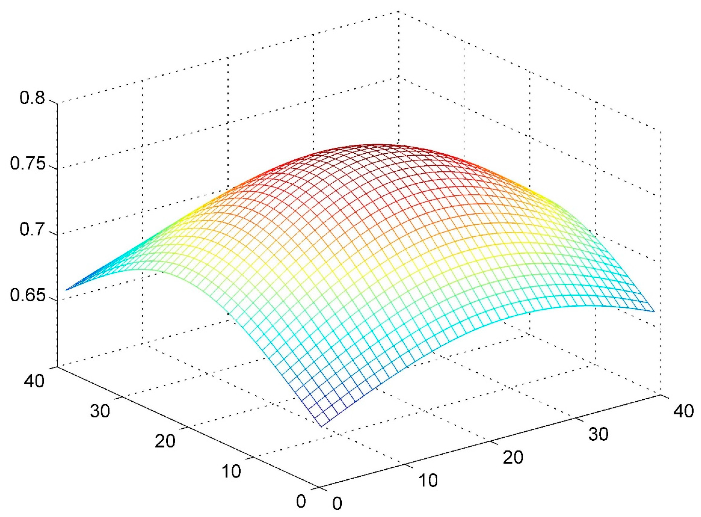
In addition, the geometrical registration between the MODIS and Landsat data is logical. Most data fusion models ignore mismatches or they simply aggregate the fine-resolution image to the coarse-resolution scale, before registration at the coarse-resolution scale, which introduces errors because the unmixing process and the prediction step are both conducted at the fine-resolution scale. In the proposed method, we employ a correlation coefficient to evaluate the agreement of the two datasets and the shifted location with the maximum correlation coefficient is regarded as the final registration result. The proposed registration method helps to improve the global accuracy.

Moreover, the assumptions of the NDVI-BSFM are more appropriate. STARFM and other models assumes that the difference between a Landsat measurement and its corresponding MODIS measurement is constant, but this assumption is tenable only when the paired DOY is very close to the predicted DOY. Therefore, nearby fine-resolution observations are required when using STARFM and similar models. In the proposed method, the differences between MODIS and Landsat data are assumed to change with time, where the difference is greater when the NDVI is larger. Under this assumption, paired NDVI on a distant date can also be used to obtain effective predictions. Therefore, the theoretical basis of the NDVI-BSFM allows the selection of paired data on a distant date. When nearby observations are not available, the NDVI-BSFM can obtain better results than other models. In addition, if nearby observations are available, then the nearby pairs are assigned greater weight compared with the distant pairs according to the definition of the weight.

Finally, in the prediction step, unlike STARFM, which uses weighted similar pixels in a neighborhood to predict the value of the central pixel, NDVI-BSFM only uses the predicted pixel, thereby retaining the individual characteristics of each pixel and protecting the predicted image from fuzziness. STARFM-like models need to employ neighboring pixels because the value of a Landsat pixel is not usually a constant distance from the value of its corresponding MODIS pixel as most MODIS pixels are heterogeneous; therefore, it is essential to obtain the regression relationship between the central Landsat pixel and the local MODIS pixels depending on many other similar Landsat pixels in the surrounding area. When the neighboring pixels are considered, the estimators are more reliable and continuous but also hazier. However, the original MODIS NDVI in STARFM is replaced by the initial NDVI in NDVI-BSFM. The initial NDVI at Landsat scale is obtained by Bayesian unmixing using the surrounding MODIS pixels, it is a type of downscaled NDVI product with patchy effects, where the difference between the real NDVI of a Landsat pixel and the corresponding initial NDVI is relatively small and regular, and hence the relationship between the Landsat NDVI and the initial NDVI summarized on the paired dates for a Landsat pixel is sufficient to predict the NDVI of the pixel itself. The NDVI image estimated by NDVI-BSFM appears to be much clearer without employing weighted averaging of the neighborhood, which acts as a spatial filter. To ensure spatial continuity, the proposed method uses prior information to constrain the unmixing process and to decrease the patchy effects at MODIS scale, where the paired NDVI datasets are then used to adjust the estimators, and the patches are barely visible after applying these two strategies.

The NDVI-BSFM also has several limitations and constraints. First, the NDVI-BSFM is fairly computationally intensive and should be simplified in future studies. Second, several parameters need to be set in the NDVI-BSFM, including the unmixing window size and the ${\mathsf{\sigma }}_{ratio}$, which indicates the relative importance of the prior information and the observations when the Bayesian unmixing process is conducted. These non-automatic parameters might limit the automation of the process during mass production. Third, similar to other data fusion models, the NDVI-BSFM cannot accurately detect short-term or tiny objects that are not recorded in the MODIS image at the prediction time or in any Landsat observations, and extra care should be taken if it is applied to other datasets where the coarse-resolution and fine-resolution sensors have a nonlinear relationship in the spectral band passes. Fourth, the angle effect of the MOD09A1 data will introduce a slight bias, and hence a semi-empirical kernel-driven bidirectional reflectance model [42] should be applied later to produce a nadir BRDF-adjusted surface reflectance product, which is more consistent with the Landsat surface reflectance product. Finally, the proposed method relies on quality control for MODIS NDVI data, so an auxiliary quality control method needs to be developed based on the fact that inaccuracy exists in the MODIS PQF. Moreover, the need for an accurate and comprehensive land cover map that differentiates all main NDVI classes is also a critical issue in complex environmental situations.

Note that the prediction accuracy varies with the selection of input image pairs because different input image pairs can have different MODIS-to-Landsat relationships, which are crucial for the Landsat-like NDVI predictions. To investigate the influence of input data pairs with different temporal distribution on NDVI-BSFM performance, various numbers and combinations of input data pairs in the Huailai area were used as base images to predict Landsat-like NDVI images on DOY = 238. Comparison of Test 1, Test 2, Test 3 and Test 4 in

Table 5. RMSE of the NDVI-BSFM predictions using different temporal distribution of input image pairs when predicting a Landsat-like NDVI image on DOY = 238 in the Huailai area.

Test Name	DOY of Input Image Pairs				RMSE
	94	206	286	318
Test 1	√				0.1330
Test 2		√			0.0665
Test 3			√		0.1274
Test 4				√	0.1345
Test 5		√		√	0.0654
Test 6	√			√	0.1268
Test 7	√	√	√		0.0647
Test 8	√	√	√	√	0.0646

shows that input image pairs with different temporal attributes bring different knowledge to the model, thus contributing to different accuracy. The input image pair on DOY = 206 provided the most accurate knowledge because the RMSE of Test 2 was much smaller than those of Test 1, Test 3 and Test 4, indicating that an input image pair which is temporally closer to the prediction date is more reliable. In Table 5, it is obvious that tests involving the input image pair on DOY = 206 (Test 2, Test 5, Test 7 and Test 8) consistently achieve high accuracy because indicators on DOY = 206 played decisive roles according to the weighting formula. Moreover, from Test 2, Test 5, Test 7 and Test 8, it is apparent that RMSE decreased slightly as the number of input image pairs increased. However, a comparison between Test 2 and Test 6 reveals that the selection of the input image pairs is more important than the number of these pairs. In brief, the acquisition of temporally close observations can provide substantial benefits, not only in NDVI-BSFM, but also in other data fusion models, including STARFM.

6. Conclusions

In this study, we described the theoretical basis, implementation, and performance of a new NDVI fusion algorithm called NDVI-BSFM for building frequent Landsat-like NDVI datasets by integrating MODIS and Landsat NDVI data. The multi-year average MODIS NDVI time series for each land-cover type is used to constrain the unmixing process for the MODIS NDVI observations in a Bayesian framework to obtain the initial downscaled NDVI, before applying a rebuilding model, which uses the relationships between the paired initial NDVI and Landsat NDVI on other dates to generate high spatial and temporal resolution Landsat-like NDVI datasets. Compared with existing methods, including the well-regarded STARFM, ESTARFM and FSDAF, NDVI-BSFM has four main advantages according to the experiments. First, the NDVI-BSFM can produce more accurate synthetic fine-resolution NDVI products (with the average absolute difference less than 0.05) in general conditions. Second, the NDVI-BSFM has a mechanism for resisting error propagation from coarse-resolution NDVI with poor quality on the prediction date, which makes the NDVI-BSFM more robust with wider adaptability. Third, the NDVI-BSFM can preserve the contrast between neighboring pixels, so the NDVI images produced using this method are always clear with rich spatial details. Finally, the NDVI values produced by NDVI-BSFM are usually smooth in the time dimension, which makes the images appear more natural in agreement with vegetation phenology. Given these advantages, we conclude that the NDVI-BSFM can obtain better results than existing methods.

In summary, the NDVI-BSFM proposed in the present study has various advantages and improves the capability for producing frequent Landsat-like NDVI datasets. This capability may contribute greatly to applications that require NDVI products with both high spatial resolution and frequent coverage, such as the monitoring of ecological dynamics, land cover mapping and change detection, and biogeochemical parameter estimation. Moreover, the concepts employed by NDVI-BSFM should provide inspiration for further studies in the future. Like other methods, the NDVI-BSFM is not only designed for fusing NDVI data from MODIS and Landsat 8/OLI sensors, but can also be applied to other sensors and products such as reflectance data and leaf area index, although extra attention should be paid to factors such as angle effect and linear additivity in space. In future research, more effort should be made to simplify the model as well as to reduce the influence of the angle effect and the quality control bias of the MODIS NDVI.