Improving Multiyear Sea Ice Concentration Estimates with Sea Ice Drift

Abstract

Multiyear ice (MYI) concentration can be retrieved from passive or active microwave remote sensing observations. One of the algorithms that combines both observations is the Environmental Canada Ice Concentration Extractor (ECICE). However, factors such as ridging, snow wetness and metamorphism can cause significant changes in brightness temperature and backscatter, leading to misidentification of FYI as MYI, hence increasing the estimated MYI concentrations suddenly. This study introduces a correction scheme to restore the MYI concentrations under these conditions. The correction utilizes ice drift records to constrain the MYI changes and uses two thresholds of passive microwave radiometric parameters to account for snow wetness and metamorphism. The correction is applied to MYI concentration retrievals from ECICE with inputs from QuikSCAT and AMSR-E observations, acquired over the Arctic region in a series of winter seasons (October to May) from 2002 to 2009. Qualitative comparison with the Radarsat-1 SAR images and quantitative comparison against results from previous studies show that the correction works well by removing the anomalous high MYI concentrations. On average, the correction reduces the estimated MYI area by 5.2 × 10⁵ km² (14.3%) except for the April–May time frame, when the reduction is larger as the warmer weather prompts the condition of the anomalous snow radiometric signature. Due to the long-lasting (i.e., from one to several weeks) effect of the warm spells on FYI, the correction could be important in climatological research and operational applications.

1. Introduction

Arctic sea ice extent has decreased by over 4% per decade from 1979 to 2010 [1], while the declining rate for the multiyear ice (MYI), ice that survives at least one summer melt, is much larger, 9%–15% per decade in the past three decades [2,3,4,5,6,7]. In late 1970s, MYI occupied two thirds of the Arctic Basin. In comparison, over two thirds of the Arctic Basin is now covered by first-year ice (FYI) [8,9]. This reversal proportion of ice cover impacts the weather and climate through different radiation and dynamic properties [10,11,12].

After every summer in the Arctic, seasonal ice that is thick enough can survive the melt and turn to MYI. This ice replenishes the reservoir of MYI that was depleted by ice export and summer melt. From 2005 to 2008, the Arctic MYI area has decreased by 42%, but the decline is not monotonic during the past decade [13]. The reduction of MYI area leads to increases in heat and mass exchanges between the ocean and the atmosphere. When MYI melts, it releases freshwater to the ocean, which alters the ocean stratification. More replenishment of thinner ice (young ice(YI) and FYI) is expected in areas that render void of MYI. Thinner ice is more liable to deform and melt and therefore allows larger heat and moisture flux exchange with the atmosphere [14]. This ice also allows greater mobility of the ice in the Arctic Basin. It was found that positive trends of ice drift speed were common in regions with decreased MYI cover [15]. Today, in years with enhanced MYI export out of the Arctic the exported MYI cannot be replenished during the following winters and this, in turn, allows more opening and mobility of the remaining ice. This positive feedback mechanism results in even less MYI coverage over years in the northern polar seas [16,17,18]. In addition, thinner ice is easier to fracture under wind forcing, giving rise to formation of leads and cracks. All these factors may lead to different composition of the Arctic sea ice as the trend of MYI decrease and its replenishment with FYI continues. From the climate point of view, it has become critical to estimate the ratio of these two sea ice categories accurately. A physically consistent MYI time series is needed to ascertain trends of climate change.

Accurate information of MYI at small and meso-scale is also important for marine operational applications. As marine activities are expected to increase along the legendary Northwest Passage that passes through the Canadian Arctic Archipelago (CAA) and the Beaufort Sea, information about MYI in these regions is becoming increasingly desirable for oil and gas exploration as well as other natural resources exploitation. Based on the results presented in [19], the MYI flow in the CAA has increased since 2005 due to the increase of open water area in the region, which provided more leeway for the MYI inflow from the central Arctic. This should also lead to more migration of MYI from the central Arctic to lower latitudes, and that would be another reason, in addition to the warming trend of the Arctic environment, to decrease the MYI area in the central region. From a climatic point of view, a physically consistent MYI time series is needed to ascertain trends of climate change.

Several algorithms have been developed to calculate sea ice concentrations from microwave remote sensing observations, e.g., radiometers and scatterometers. Radiometers measure emitted radiation (in terms of brightness temperature), while scatterometers measure the backscattered radar signal after reflection of the surface (in terms of backscatter coefficient). A partial list of the sea ice concentration retrieval algorithms is provided in [20] with comparisons of their performances. Among them, only a few algorithms are able to distinguish different ice types and estimate their partial concentrations, e.g., MYI concentration. The methods [21,22,23,24,25,26,27] allow deriving concentrations of MYI and FYI, the method of [28] estimates thin ice and ice with snow layering types, and the method of [29] determines concentration of any given set of ice types based on the provided characteristics. The latter is known as the Environment Canada’s Ice Concentration Extractor (ECICE). It requires a priori probability distribution functions for each radiometric parameter (e.g., brightness temperature and backscatter coefficient) and each surface type. The number of radiometric parameters must be equal to or larger than the number of specified surface types.

In a validation study of ECICE [30] using combined input from passive and active microwave observations, it was found that during warm spells in spring, caused by large cyclones that brought warm air to the region, the algorithm identifies FYI as MYI. The authors attributed this anomaly to a melt-refreeze cycle over the snow-covered FYI surface. The resulting snow metamorphism and layering within the snow modifies the dielectric constant and the volume scattering. The net result is an increase in backscatter and a decrease in brightness temperature from the snow-covered FYI to values similar to those from the MYI. This leads to a sudden and wrong increase of the retrieved MYI concentration from ECICE. This observation was confirmed in [31] under similar conditions using the NASA Team algorithm based on radiometer measurements. The anomalies of the radiometric and backscatter observations make it impossible to rely solely on microwave observations to identify ice types under these conditions. Certain physical conditions should be incorporated in the ice concentration algorithm to account for the effect of warm spells.

This study suggests a correction scheme to compensate for the overestimated MYI concentrations due to the aforementioned reasons. In addition to looking at sudden radiometric changes, it utilizes ice drift to constrain the MYI concentrations within a feasible contour. The ice drift product [32,33] is derived from multi-satellite and in-situ measurements. Furthermore, the scheme examines two parameters derived from the passive microwave observations to identify and account for the effects of snow wetness and metamorphism. Although the correction is applied to MYI concentration obtained from the ECICE algorithm, it can be equally applied to the results from any other MYI concentration algorithm. Section 2 presents a short reference to the ECICE algorithm and the description of the data sets. Section 3 provides representative cases and physical interpretations of the misclassification of FYI as MYI in late winter, and Section 4 presents the correction scheme. Results and discussions are offered in Section 5, and the conclusions in Section 6.

2. The ECICE Algorithm and Data Sets

The ECICE algorithm is used to derive concentration of three ice types: MYI, FYI and YI. The algorithm starts with a linear mixing model that decomposes each radiometric observation into contributions from each surface type (in this case YI, FYI, MYI, and open water (OW)) weighted by the concentration of the surface type within the sensor’s field of view. The set of linear equations (shown as Equation (1) in [30]) is incorporated with a set of constraints to construct a cost function, in which the partial concentration of each ice type is an explicit parameter. The constraints include an equality condition, which stipulates that the sum of all partial concentrations must be 100%, and a set of inequality constraints, which stipulate that partial concentration of each surface type must be between 0% and 100%. The optimal solution minimizes the cost function [29]. Instead of using a single set of tie points (typical radiometric values for each surface type of each radiometric parameter) in the linear mixing model, the algorithm uses a large number of sets of characteristic values (typically 1000), and each set represents a possible (but not necessarily a typical) value of the given radiometric parameters for each surface type (the input radiometric parameters are described below). A random number generator is used to generate each set of characteristic values with the known distribution, which is based on sampling each parameter over homogeneous areas of the relevant surface type. The set of characteristic values are then used to obtain a possible optimal solution. The final optimal solution (concentration of ice types for each pixel) is generated from the 1000 possible solution using a weighted average of all solutions.

The ECICE algorithm is used in this study with four input observations: backscatter coefficients ${\sigma }_{hh}^0$ and ${\sigma }_{vv}^0$ from the SeaWinds Ku-band scatterometer onboard QuikSCAT, along with brightness temperatures at the 36.5 GHz horizontal and vertical polarization channels ($T{b}_{37h}$ and $T{b}_{37v}$) from the Advanced Microwave Scanning Radiometer/EOS (AMSR-E). Seawinds/QuikSCAT is a 13.4 GHz (Ku-band) conically scanning pencil-beam scatterometer, operating from July 1999 to November 2009. It has two beams, each with a wide range of azimuth angles. The inner beam is horizontally polarized at an incidence angle of 46°, whereas the outer beam is vertically polarized at an incidence angle of 54° [34]. The sensor measures normalized cross section or backscatter values in dB over a swath width of 1800 km. AMSR-E on board the NASA Aqua satellite is a six-frequency dual-polarized radiometer, operating from May 2002 to October 2011. Brightness temperature of different channels from AMSR-E has been widely used in deriving sea ice information [35,36,37,38]. In addition to $T{b}_{37h}$ and $T{b}_{37v}$, which are input to ECICE, a linear combination of brightness temperature from the 18.7 GHz and 23.8 GHz channels is used to filter the open water pixels.

Both data sets were obtained from the Microwave Earth Remote Sensing (MERS) laboratory of Brigham Young University (BYU). The data are enhanced and reconstructed using the Scatterometer Imager Reconstruction (SIR) resolution enhancement algorithm. The technique is presented in [39] for the scatterometer data and in [40] for the passive microwave data. It takes advantage of the spatial overlap made at different times of one day to enhance the imaging resolution, which is equivalent to the antenna-pattern deconvolution [40,41]. It also uses the multiple passes from different orbits during one day to reduce pixel noise. The resampled resolution for both datasets is 4.45 × 4.45 km². Two products from SIR-enhanced QuikSCAT exist: “slice” and “egg”. “slice” are the 12 individual radar normalized backscatter measurements for each footprint as the QuikSCAT scans over an 1800 km wide swath, which are 4–6 km long by 20 km wide. The summed measurements of the “slice” are called “egg” measurements. The descending (evening) passes “egg” product is used in this study due to its lower sensitivity to noise during the SIR process. The enhanced AMSR-E data include ascending (mid-day) and descending (mid-night) passes products. The descending passes product is used to be consistent with the QuikSCAT data. The data set used in this study covers the winter months (October-May) from October 2002 to May 2009, which is the winter overlapping period between the two sensors.

Polar Pathfinder Daily 25 × 25 km² resolution Equal Area Scalable Earth Grid (EASE-Grid) Sea Ice Motion Vectors, Version 2 [32,33] from the National Snow and Ice Data Center (NSIDC) is used in this study. It is one of the most comprehensive ice drift products for the Arctic Ocean, providing daily gridded ice motion vectors and the estimated error variance from November 1978 to December 2012. The vectors are obtained from a variety of satellite-based radiometers such as the Advanced Very High Resolution Radiometer (AVHRR), the Scanning Multichannel Microwave Radiometer (SMMR), the Special Sensor Microwave Imager (SSM/I) and AMSR-E. The observations are merged with the buoy data from the International Arctic Buoy Program (IABP) and wind data from the National Centers for Environmental Prediction (NCEP) analysis, using a co-kriging estimation method described in [42]. The AVHRR data is only used until December 2004 and all passive microwave remote sensing data are used during their operation time (SMMR 1978–1987, SSM/I 1987–2006, SSMIS 2007–2012, AMSR-E 2002–2012). For this study, the ice drift data were resampled to the same grid spacing as the QuikSCAT and AMSR-E data (4.5 × 4.5 km²).

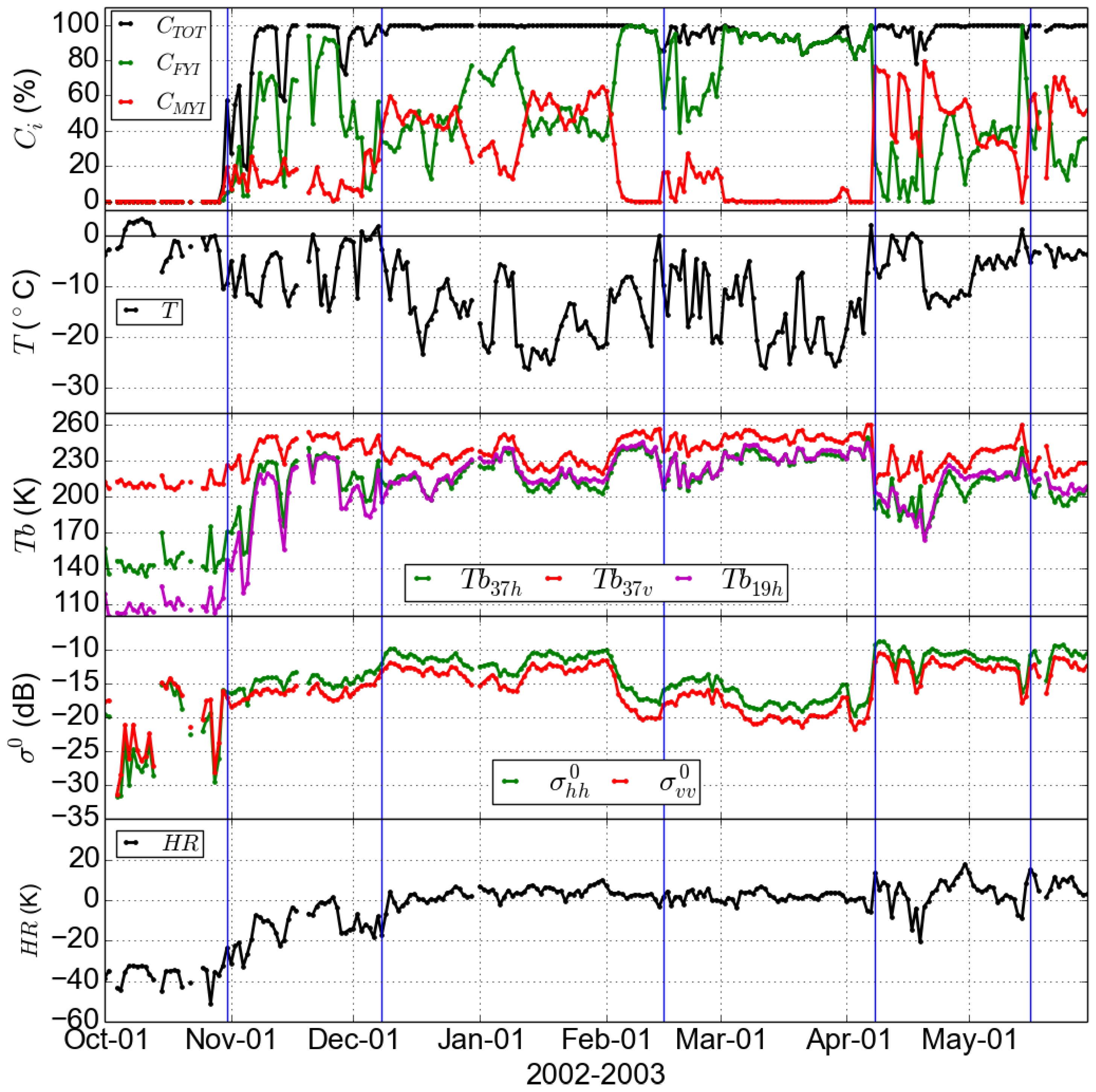
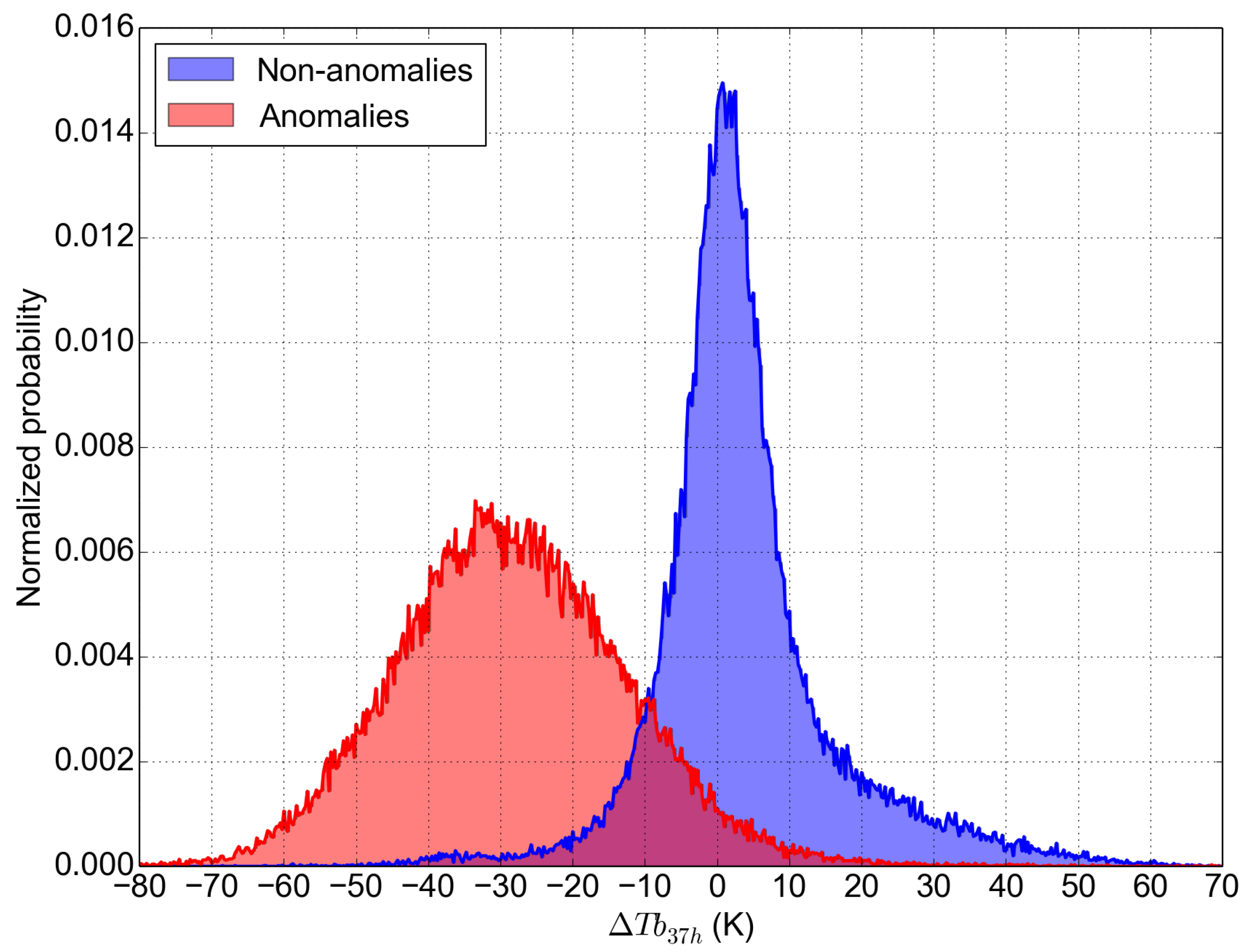
3. Misclassification of FYI as MYI

As described in [30], when the atmospheric temperature approaches the melting point, the MYI concentration retrieval from ECICE shows a sharp increase. Moreover, sudden appearance of MYI near the ice edge is frequently observed in the output maps. These observations cannot be explained by the motion of MYI because the large distance renders it infeasible. Formation of MYI in new locations is also not possible in the spring. Hence, the sharp increase of MYI concentration (accompanied with an equal drop in FYI concentration) is regarded as misclassification. These anomalies are observed mainly in late winter and early spring (from February to May) and may last for a few days or weeks or sometimes for the rest of the season. During such periods, the brightness temperature from FYI decreases and the backscatter increases to values close to those of MYI. Unlike the radiometric effect of warm spells on the snow-covered MYI [30,43,44], which ends after the low temperature returns, the effect on the snow-covered FYI shows long-term or irreversible behaviour even when the warm spell abates. One explanation can be that the snow on FYI retains some salty solute, which is partly or totally drained when the snow becomes wet. Such irreversible processes renders the misclassification of FYI as MYI in winter/spring more durable even when the warm spell abates. A correction scheme based on ice motion is suggested and described in the next section.

An example of the described anomaly is presented in Figure 1. On 7 April 2003, warm air is advected over the Barents Sea. On 8 April, non-zero MYI concentration appears suddenly west of Novaya Zemlya and the concentration approaches 100% on 9 April, whereas the corresponding FYI concentration decreases to near 0%. The identification of MYI in this region is not correct since it can not have grown locally or been advected from the main pack to such a far distance in two days. Thus the increasing MYI concentrations from 8 April to 21 April west of Novaya Zemlya must be incorrect. This anomaly stays in the region for over three weeks and disappears until 13 May.

Figure 2 shows the daily records of MYI and FYI concentrations, air temperature, brightness temperature and backscatter from all pixels within an area bounded by 76.75°–77°N latitude and 29°–30°E longitude (red start in Figure 1a) in the Barents Sea from 1 October 2002 to 31 May 2003. The five vertical blue lines in the figure correspond to the days with sudden increases of MYI concentration. The first case occurs at the end of October, when concentration of MYI and FYI both increases from 0% to about 20%. This increase is not caused by misclassification but ice advection from nearby regions. From 1 December to 9 December, the MYI concentration increases by about 50%. Shortly before this MYI increase event, air temperatures rise above 0 °C and drop to cold temperatures again when the event starts. This melt-refreeze cycle leads to persistently increasing QuikSCAT backscatters, while the AMSR-E brightness temperatures strongly increase from one day to the next before the event but return to values similar to the ones before the event on 9 December. A potential explanation for this situation is the combined effect of ice deformation and snow melt-refreeze cycle. As confirmed from the daily sea ice drift product of NSIDC, direction of ice drift changes abruptly from one day to the next, which is likely to cause ice deformation in the studied area and can be considered as an evidence for the hypothesis. The third case happens on 15 February, when the MYI concentration increases from 0% to 20% and the total ice concentration keeps unaltered. Again, the air temperature rises to near zero shortly before the event and is followed by cold temperatures (about −10 °C), which indicates a melt-refreeze episode on FYI. This results in decreased brightness temperatures and increased backscatters, which causes the false MYI concentration increase. Similar conditions can be found in the cases of 8 April and 16 May.

The described increase of MYI concentration is expected to be replicated by other MYI concentration retrieval algorithms. For example, [31] noted that increased volume scattering after the melt-refreeze episodes in late winter results in unrealistic high estimates of MYI concentration from the NASA Team algorithm, which uses radiometer measurements only. The radiometric responses to the melt-refreeze events lead to overestimates of MYI concentration from other microwave-based ice retrieval algorithms as well. Hence the suggested correction in the current study is also suitable for applications of any other microwave-based ice retrieval algorithm.

Microwave emission and scattering from snow is affected by snow density, salinity, temperature, wetness and grain morphology [46]. Snow on FYI is characteristically (and therefore radiometrically) different from snow on MYI. The FYI surface is usually saline, and the overlain snow wicks up the brine through capillary action. When air temperature approaches sub-zero values during the freezing season, snow becomes wet. If the temperature decreases again, liquid water in the snow will aggregate small crystals to coarsely grained clusters with larger voids between the grains. These are permanent changes. On the other hand, snow on MYI is saline-free and has mostly metamorphosed into crystalline structure since it has been exposed to cycles of high and low temperatures. In this case, the effect of a warm spell will be manifested in measurable wetness, and if the temperature decreases again the snow will retain its physical structure and composition. This makes it easier to account for the effect of warm air temperature on snow on MYI as described in details in [44].

The impact of air temperature changes (warm/cold cycles) on the microwave observations is complex and remains unclear. Findings from the many studies of snow on sea ice continue to raise questions more than providing answers [47]. A few guiding notions to assist in the interpretation of the above-mentioned anomalies of microwave-based ice concentration retrieval are summarized below. Two factors are addressed: snow wetness and snow metamorphism into larger grain size.

When there is wet snow on sea ice, the emitted radiation is less at the horizontally-polarized channel of 19 GHz than 37 GHz [48,49]. The difference can be used as an indicator of the amount of snow wetness [50,51]. For radar backscatter, snow wetness affects both surface and volume scattering. Surface scattering increases and volume scattering decreases as snow wetness increases. The net effect is a significant decrease of backscatter as the snow wetness increases to about 3% then it stabilizes [52]. A study presented in [53], however, shows that the melt onset of FYI is marked by a rapid increase in backscatter as the wet snow becomes more reflective of the microwave energy. Therefore, the observed misidentification of FYI as MYI would probably be attributed to wet snow with its combined effect on both emitted microwave and radar backscatter signal (recall that both observations are used in the retrieval). Snow metamorphism increases the volume scattering, resulting in decrease of emissivity (and therefore brightness temperature) and increase of radar backscatter. The effect of snow grain size on radar backscattering has been studied by [54] using a multiple scattering model. The authors showed an increase of backscatter coefficient at vertical polarized Ku-band from −15 dB to −2 dB as the radius of snow grains increases from 0.5 mm to 1.5 mm. This brings the backscatter up to typical values of MYI and that is what triggers the observed anomalies. The correction scheme accounts for the effects of snow wetness and metamorphism with two different parameters as will be shown in the next section.

4. The Correction Scheme

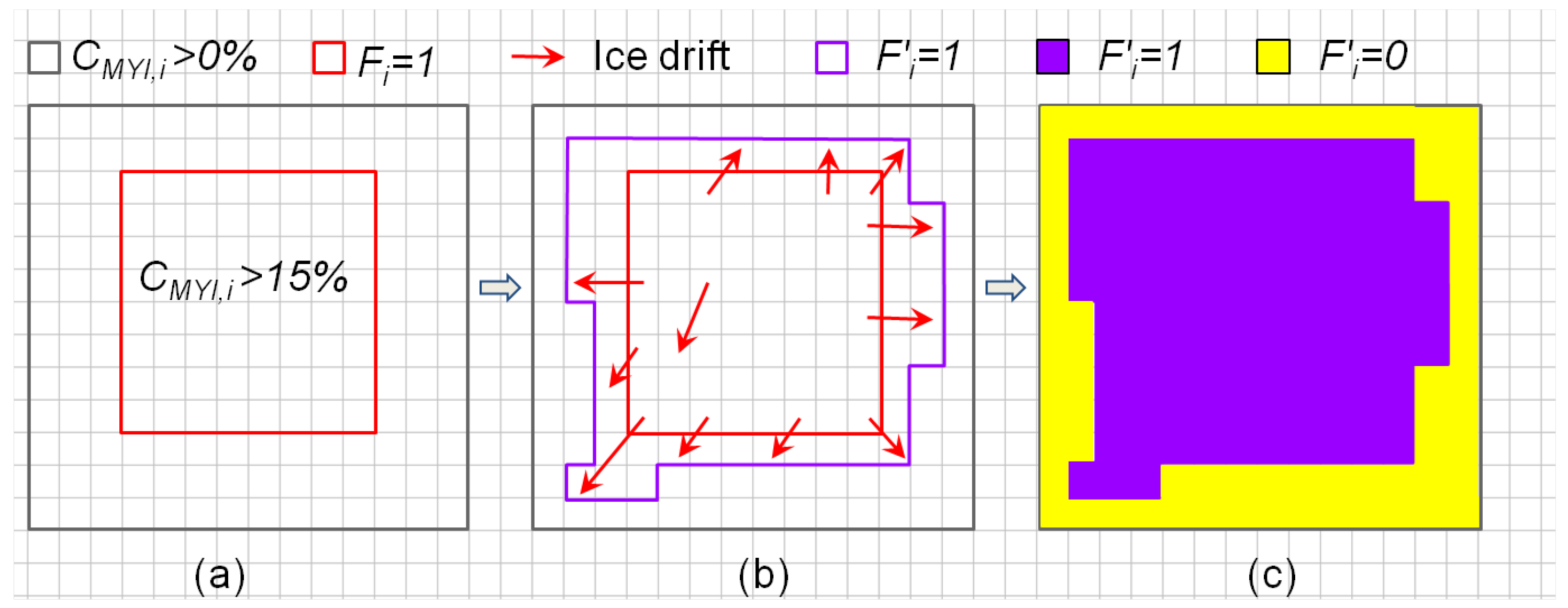
4.1. Outline of the Correction Scheme

As described in Section 3, ice deformation, snow wetness and metamorphism can cause significant changes in microwave brightness temperature and backscatter, leading to misidentification of FYI as being MYI, the effects of which are considered here. In many situations the affected pixels are found to be located far from the main pack ice, particularly in the eastern Arctic such as the Laptev Sea, the Barents Sea, and the Greenland Sea. This is expected because near- or above-freezing temperatures are more frequently encountered in these regions. Warm temperatures enhance the possibility of the anomalous microwave signatures. For a given day, pixels with MYI concentration over 15% are identified. These pixels constitute the so-called MYI domain (the red box in Figure 3a) of the given day. With the daily ice motion vector, this MYI domain is expanded accordingly to produce a new MYI domain (the purple contour in Figure 3b). For pixels that are located outside the new domain (the yellow region in Figure 3c), MYI concentrations of the second day are corrected without checking any radiometric indicator of snow wetness and metamorphism (described later in this section). For pixels within the new domain (the purple region in Figure 3c), the indicators should be checked to confirm that the originally-estimated concentrations (in our case from the ECICE algorithm) are indeed anomalous (pixels have abrupt increases of MYI concentrations on the two successive days) and therefore needs correction. The correction proceeds as follows.

First, for each pixel, a flag, $F_i$, is defined. $F_i=1$ when the MYI concentration is over 15% on day i. Otherwise, $F_i=0$. Pixels with $F_i=1$ constitute the originally-estimated MYI domain of day i (the red box in Figure 3a). For pixels within the domain, daily ice drift is used to calculate the expected displacement after one day (i.e., on day i + 1). The MYI domain is expanded according to the displacement, consequently generating a new MYI domain. It should be noted that the MYI domain is only expanded when the examined pixel inside the original MYI domain is advected out of it. Pixels within the new domain are indicated with $F_i^{\prime }=1$ (the purple region in Figure 3c), whereas those outside the domain have $F_i^{\prime }=0$ (the yellow region in Figure 3c). $F_i^{\prime }=0$ means that there should be no MYI on day i + 1, whereas $F_i^{\prime }=1$ implies that there could be MYI on the next day (i.e., day i + 1) based on the estimation from ice motion and previous concentrations. The explicit correction procedures for pixels with $F_i^{\prime }=0$ and $F_i^{\prime }=1$ are described in the second and third step, respectively.

Second, for pixels outside the new MYI domain ($F_i^{\prime }=0$), the correction starts with the examination of the distance from the pixel to the boundary. We calculate the distances from this pixel to all the pixels within the estimated domain ($F_i^{\prime }=1$). If the minimum distance is more than 4.45 km (one pixel), presence of MYI is not allowed and the MYI concentration on day i + 1 is replaced with 0%. If the minimum distance equals to 4.45 km, the MYI concentration is replaced with that of the previous day but only if the difference between the concentration from day i + 1 and day i ($\Delta C_{MYI}=C_{MYI,i+1}-C_{MYI,i}$) exceeds a certain threshold ($\Delta C_M$). The value of $\Delta C_M$ will be determined in Section 4.2. This margin is introduced to account for uncertainties of the ice drift product from NSIDC, which range from 1–2 cm/s (about 1–2 km/day) [55,56].

Third, for pixels that are located within the expected MYI domain ($F_i^{\prime }=1$), a correction that accounts for snow wetness and metamorphism is applied to the pixels that have $\Delta C_{MYI}>\Delta C_M$. In [51,57], the authors used a spectral difference, the horizontal range ($HR=T{b}_{19h}-T{b}_{37h}$), to detect snow melt onset on sea ice. When HR is below −10 K, liquid water is assumed to be present in the snowpack, leading to overestimation of MYI concentration. In the correction procedure, the MYI concentration is replaced with that of the previous day when HR < −10 K. In addition, as mentioned before, larger grain size in the snowpack causes decreases of brightness temperature. In previous studies [50,51], the authors interpreted an abrupt decrease in brightness temperature from one day to the next ($\Delta T{b}_{37h}$) as being caused by snow metamorphism. In the present correction scheme, if the decrease in $T{b}_{37h}$ exceeds another threshold ($\Delta T{b}_0$), the MYI concentration is replaced with that of the previous day when $\Delta C_{MYI}>\Delta C_M$.

The correction scheme involves two phases. The first phase modifies the anomalous MYI concentration when the pixel is located far enough outside the expected MYI boundary. This is referred to as correction prompted by ice drift. The second phase is applied to pixels inside the expected boundary and referred to as correction prompted by snow wetness/metamorphism. The relative weight of these two components is presented in Section 5.1. It should be mentioned that the scheme is applied to the MYI concentration retrieval from ECICE after the application of an earlier correction [44] that accounts for sudden drop of MYI concentration (i.e., negative MYI concentration anomaly). These two correction schemes are independent regarding the different MYI anomalies that are accounted for: negative anomaly for the earlier one and positive anomaly for the correction presented here. In the earlier correction [44], it has been found that this negative MYI anomaly occurs mainly in September-October, which is triggered by the atmospheric temperature that approaches the melting point of snow and is restored by interpolation of the concentrations before and after the anomaly events.

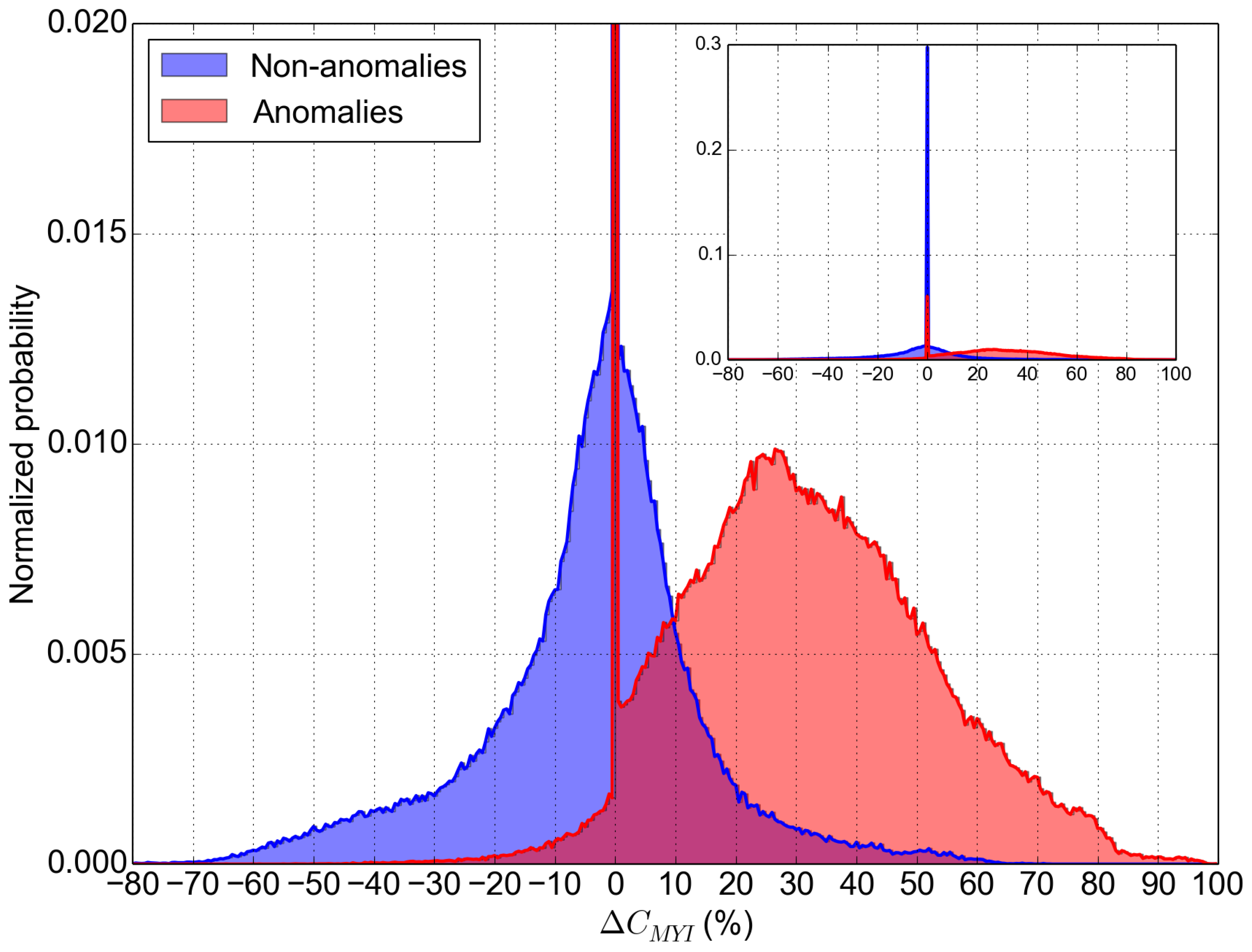
4.2. Threshold Adjustment

Two thresholds, $\Delta C_M$ and $\Delta T{b}_0$, are used in the correction procedure. $\Delta C_M$ indicates the sudden increases of MYI concentrations beyond which the increase can probably be anomalous, whereas $\Delta T{b}_0$ is the value above which the sudden decreases in $T{b}_{37h}$ is considered to be caused by snow metamorphism.

In order to determine the thresholds, we selected samples for anomalies under the condition of unrealistic large increases of MYI concentration along with abrupt decreases of brightness temperatures (about 260,000 data points in total). The selection is based on visual interpretation for maps of MYI concentration and brightness temperature. For comparison, the same pixels were selected from the adjacent days outside the anomalies period. Probability distributions of $\Delta C_{MYI}$ and $\Delta T{b}_{37h}$ from these samples from 2002 to 2009 are shown in Figure 4 and Figure 5, respectively. Red curves represent the distribution of the anomalies, and blue of the non-anomalies.

In Figure 4, the value best separating the two clusters of anomalies and non-anomalies is approximately 10 percent ($\Delta C_{MYI}$). In the second step of the correction procedure, $\Delta C_M$ is used to account for uncertainties of the MYI concentration retrieval and the ice drift product. Uncertainty of the MYI retrieval from ECICE can reach 5–10 percent, which asserts that $\Delta C_M$ should be larger than 10 percent. Among the non-anomalies, 11.9% of the samples have $\Delta C_{MYI}$ over 10 percent, while only 5.0% of them have $\Delta C_{MYI}$ more than 20 percent. We consider 5% of the non-anomaly values to be falsely corrected (false positives) by the scheme to be acceptable. Therefore, 20 percent is selected as the threshold $\Delta C_M$.

The same anomalies and non-anomalies samples are analyzed in Figure 5 to determine the threshold $\Delta T{b}_0$. It is found that −10 K is the value that best distinguishes the anomalies from non-anomalies. Among the non-anomalies, 7.42% of the samples have decreases of $T{b}_{37h}$ more than 10 K from one day to the next, whereas only 2.17% of them have $\Delta T{b}_{37h}$ below −20 K. Again, in order to constrain the amount of non-anomalies to be misidentified as anomalies and over-corrected by the correction (false correction), −20 K is selected as the threshold $\Delta T{b}_0$.

5. Results and Discussions

5.1. General Observations

As described in Section 4, the majority of the anomalous MYI pixels are found to be located far from the main MYI pack. The correction of these pixels is performed using the ice drift data. On the other hand, anomalous pixels within the ice pack are corrected based on the snow wetness/metamorphism radiometric conditions. The percentage of each correction phase is given in

Table 1. Relative weight (%) of the two components involved in the correction scheme.

Correction Phase	Oct	Nov	Dec	Jan	Feb	Mar	Apr	May
Ice drift	98.64	99.52	99.69	99.73	99.80	99.85	99.78	99.74
Snow wetness/metamorphism	1.36	0.48	0.31	0.27	0.20	0.15	0.22	0.26

, averaged for each month over the seven studied years. It is apparent that most of the affected (anomalous) pixels are located far from the expected MYI boundary and can be corrected with the ice drift data. However, it should be noted that the ice drift correction is applied before the snow wetness/metamorphism correction, thus higher percentage values can be expected.

Examples of the anomalies and the results after correction are presented in Figure 6. The top and bottom panels show the estimated MYI concentration before and after correction, respectively. For the days shown in the figure, the MYI concentration maps after applying the temperature-based correction [44] are almost identical to those generated from ECICE. This means that the radiometric anomalies that cause erroneous identification of MYI as FYI as discussed in [44] are rarely encountered in the shown dates. The figure shows anomalous estimates of MYI (high concentration) in areas that should contain FYI only (based on observations from successive daily MYI concentration maps). The increase occurs usually suddenly between one day and the next (as demonstrated in Figure 1) and is attributed to the reasons explained in Section 3. In the first example of 9 April a pocket of high MYI concentration is shown between Novaya Zemlya and Svalbard islands. Same anomalies appear in the map of 26 April in addition to other anomalies along the southern coast of Greenland and the Asian coast (east of Scandinavia). The map of 9 May shows the anomalous MYI concentrations in the Chukchi Sea and around the southern area of the Baffin Island, while similar anomalies are apparent in the map of 18 May in the Barents Sea and Bering Strait. Many of such anomalies remain for several days and some continue for the rest of the season. Most of them are removed by the correction scheme presented here as shown in the bottom panel.

The correction preserves some MYI along the ice drift routs, from the central Arctic (where the core volume of MYI exists) to southern latitudes. One such route is Transpolar Drift Stream (TDS), which moves ice from the Siberian coast across the Arctic basin to drift along the east coast of Greenland. Other routes through the Canadian Arctic Archipelago are also revealed in Figure 6. MYI remains also after correction in the Nares Strait between Greenland and Ellesmere Island (a well-known area usually blocked by MYI, leading to formation of the North Water Polynya [58,59]. Qualitatively speaking, these observations substantiate the reliability of the correction scheme. The correction scheme introduces a few scattered adjustments of MYI concentration in the central Arctic to account for the radiometric effects of snow metamorphism as explained before. These, however, are few and not readily visible when comparing the uncorrected against the corrected maps. In general, the correction is most pronounced in peripheral seas of the Arctic Basin. It is worth mentioning that the spatial distribution pattern of MYI concentration is preserved on all the dates in Figure 6, and the concentration decreases gradually towards the edge of the ice cover.

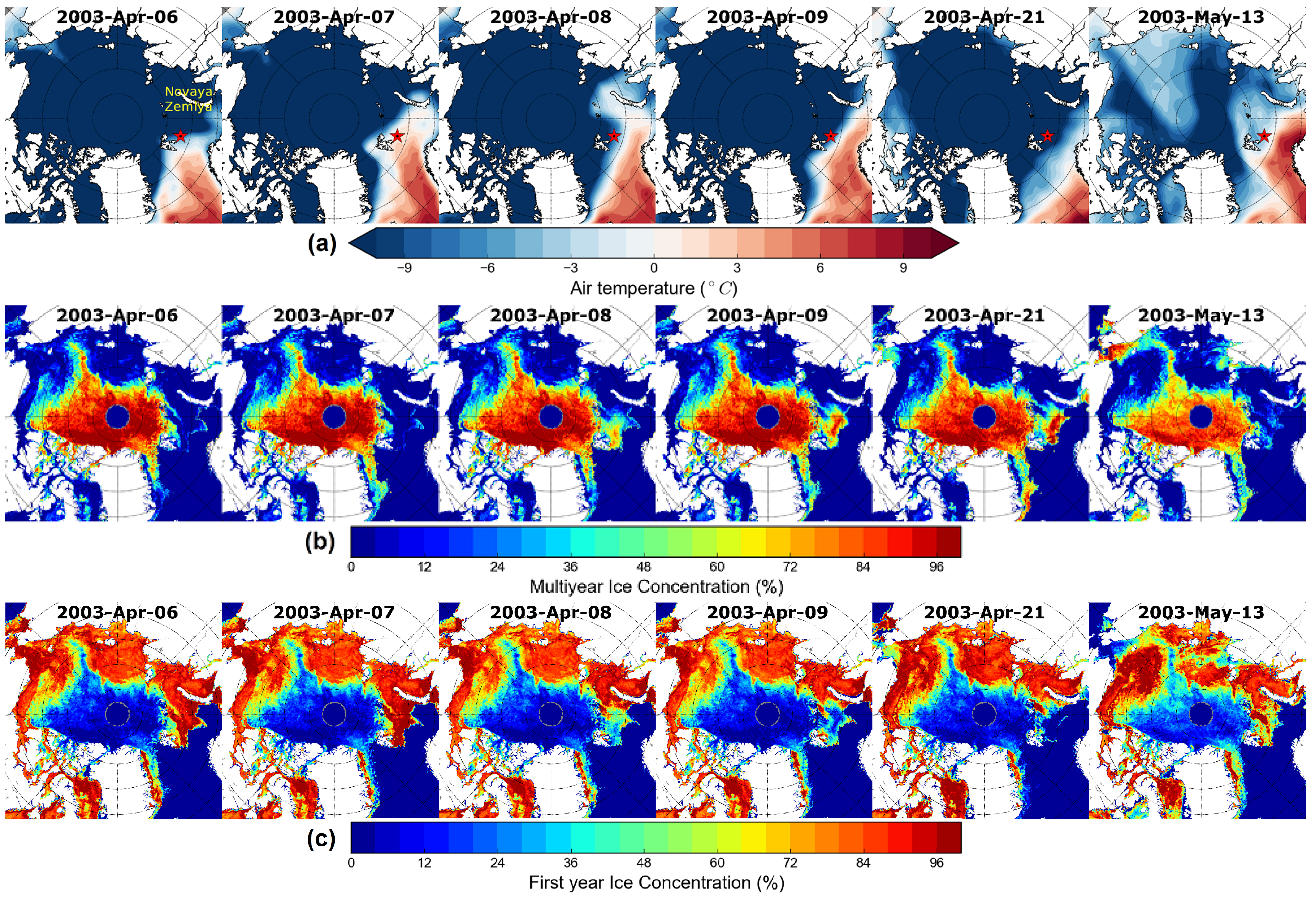
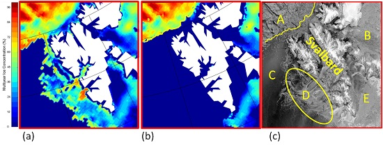
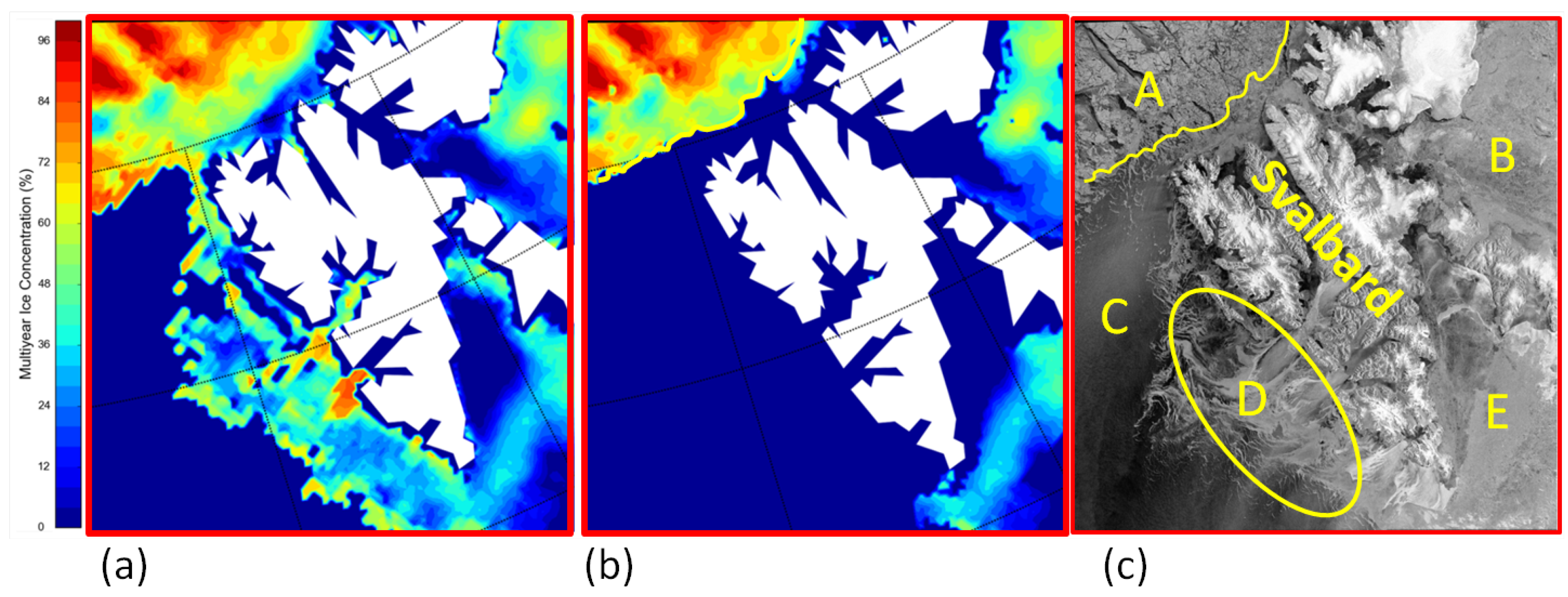
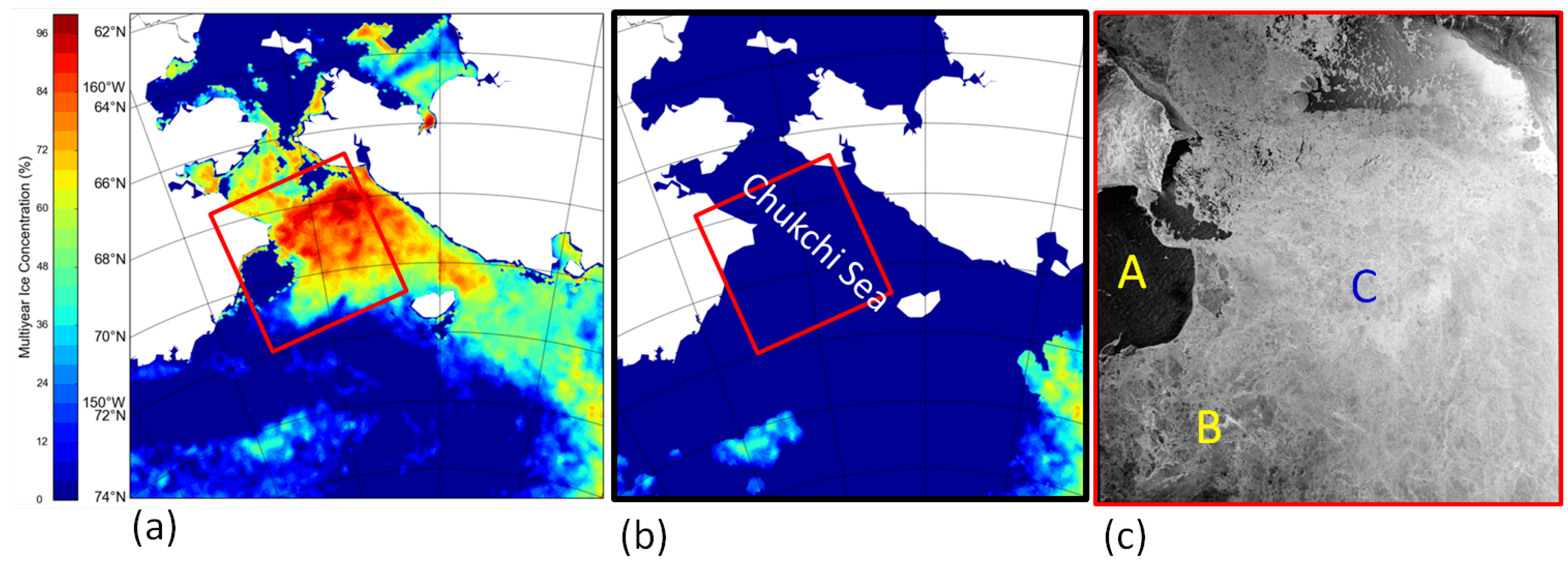
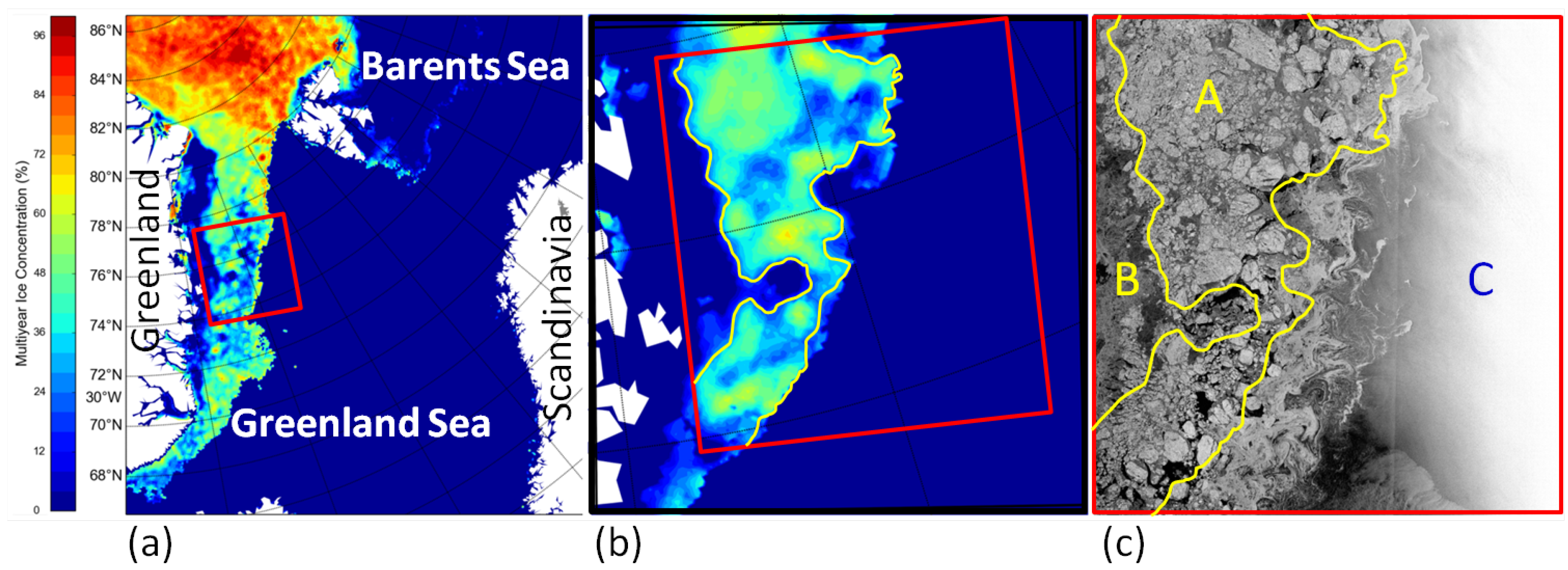
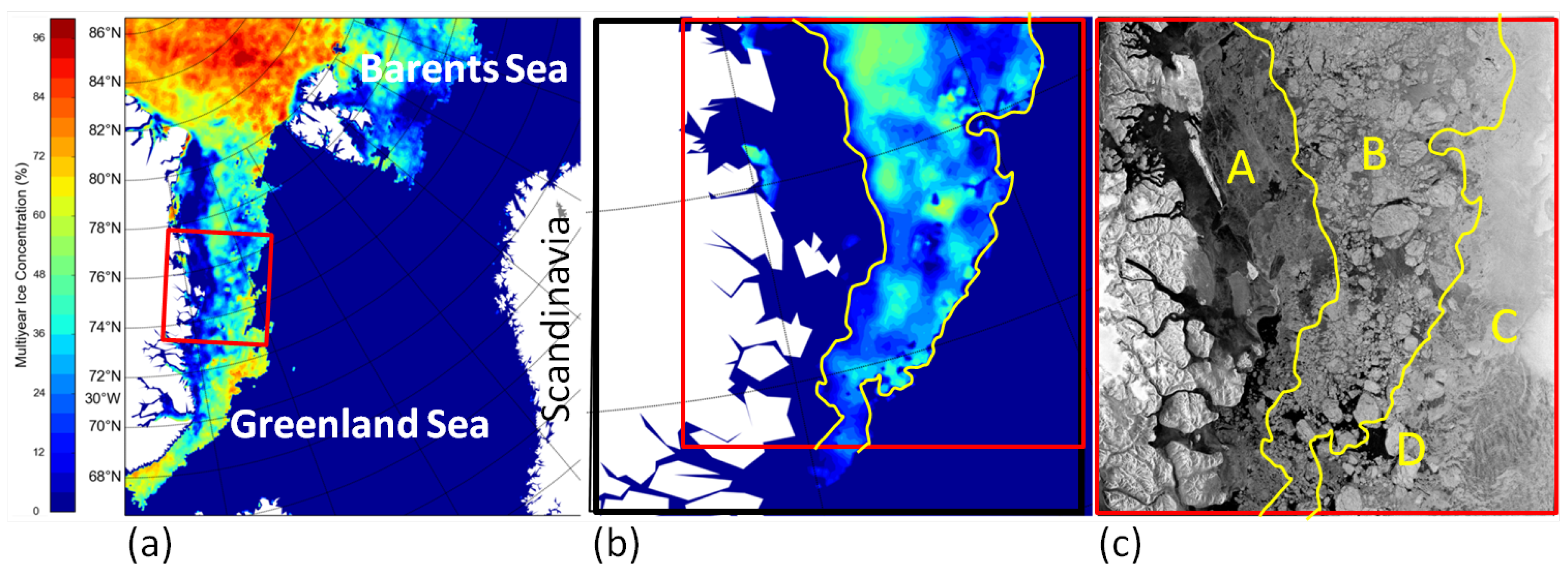
5.2. Inter-Comparison with SAR Images

This section presents qualitative comparisons of the MYI concentrations before and after corrections against information from the visual analysis of Radarsat-1 SAR images. Four case studies are presented.

Case study (1): Ice around Svalbard 

Data of 2 April 2003 are shown in Figure 7. On this day, the winds were blowing from the north and northeast to the south of Svalbard (the archipelago in the middle of Radarsat-1 frame overlaid on the MYI concentration map in Figure 7a) through the Barents Sea (about 5–10 cm/s), and the air temperatures were below −7 °C. Five areas are marked in the accompanying Radarsat-1 image. Area A contains MYI with its visible floe structure and relatively high backscatter. Areas B and E feature ice surface with relatively high backscatter and smooth texture, which appears to be FYI. Given the southward winds and the low temperatures, these three areas are most likely made up of ice that is advected from the Central Arctic. The MYI concentration maps after correction show values of 20%–90% in area A and of 10%–60% in areas B and E. These concentrations remain almost unchanged after correction (comparing Figure 7a,b in the figure). Area C appears to have open water, and it remains unaffected by the correction. The remarkable change resulted from application of the correction is visible in area D. Here, the Radarsat-1 image reveals high backscatter with streaks of low values, a typical signature of young ice streaks, which was probably generated locally due to low temperature and wind in this area. The passive microwave signature of young ice can be as low as that of MYI. Therefore, both passive and active microwave observations favored identification of MYI in this area (wrongly). This is removed after correction (Figure 7b) based on the fact that MYI in this area is found at far enough distance from the main pack ice.

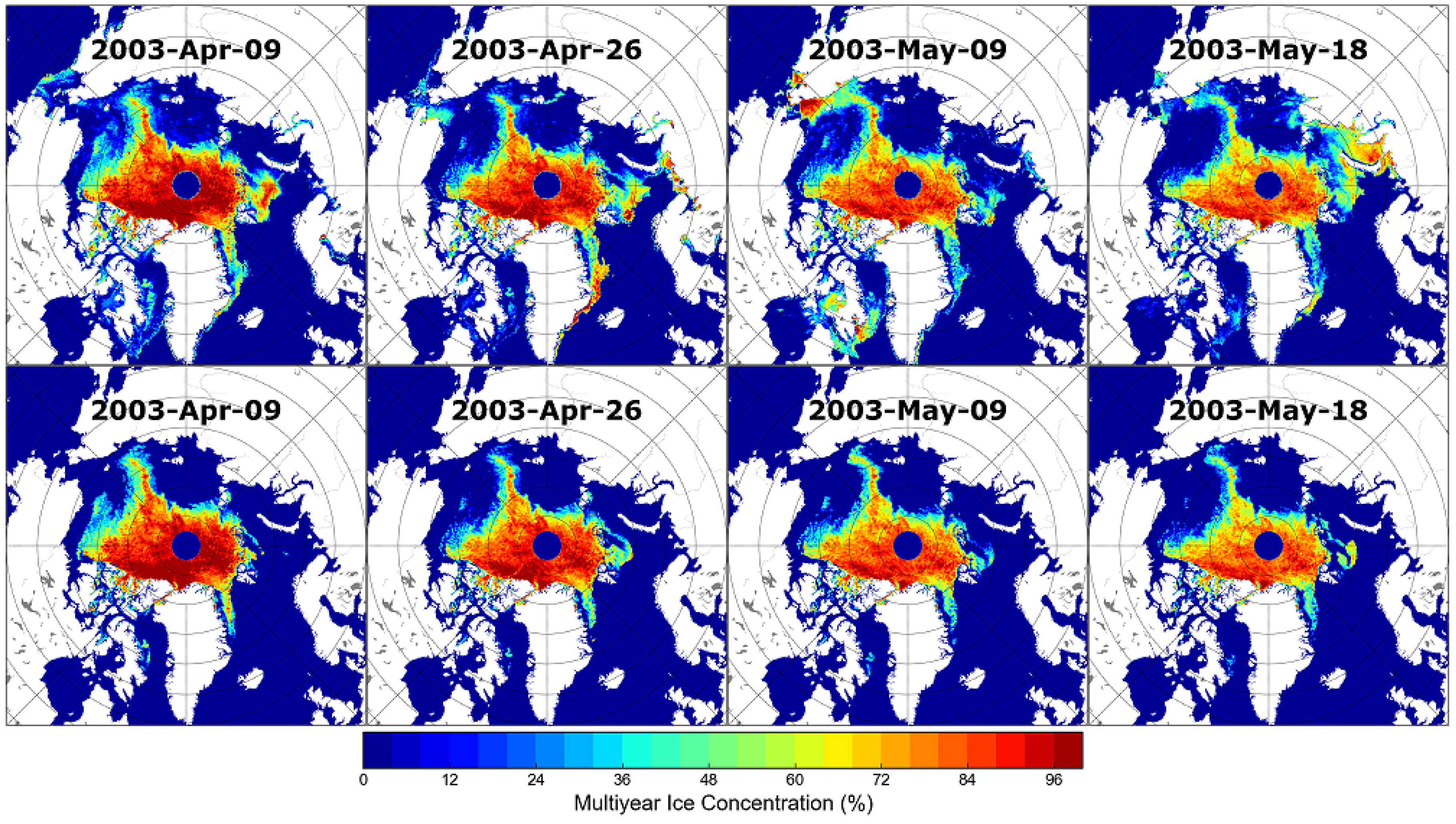
Case study (2): Ice in the Chukchi Sea 

MYI concentration maps before and after corrections, along with a corresponding Radarsat-1 image of the Chukchi Sea are shown in Figure 8. Data are generated from observations of 6 May 2003. The high MYI concentrations in the Chukchi Sea (Figure 8a) appeared suddenly on 29 April and continued with varying concentration levels until they abated on 17 May. The sudden appearance raises doubt about the authenticity, especially as the area is located far from the main MYI pack in the central Arctic. On 6 May, the temperatures were near 0 °C and the winds were generally blowing from the southeast with low wind speeds (<5 cm/s). The Radarsat-1 scene (Figure 8c) does not show any MYI with its typical attributes of high backscatter, texture and ice floe structure. Except for what appears to be a quasi-steady water surface with its dark backscatter signature (area A), the rest of the scene emerges as being of consolidated FYI sheet yet with different backscatters. Some linear pressure ridges appear against a background of darker signature in area B. The relatively high backscatter that covers the main scene (area C) can be linked to the wet snow as explained in Section 3. This area coincides with the high (and wrong) estimate of MYI concentrations from ECICE, an understandable consequence of the anomalous backscatter. Given the relative high temperatures and the minimum sea ice extent of the previous summer being distant from the Chukchi Sea, the only explanation for the possible appearance of MYI in this region is ice advection from the central Arctic. Yet, the sudden appearance of such high MYI concentration (as mentioned above) refutes this explanation. The correction scheme retained the zero MYI concentration in the region on account of its remoteness from the main MYI pack in the central Arctic.

Case study (3) and (4): ice in the Greenland Sea 

These two cases are most crucial because they present results from a highly dynamic ice regime, namely the Greenland Sea along the east coast of Greenland. This is a major route of sea ice drift from the Laptev Sea and East Siberian Sea southward, driven by the Transpolar Drift Stream (TDS) [60,61]. Since the speed of ice motion is employed in the correction scheme, the results should clearly be sensitive to its accuracy. Assessment of this accuracy in the Arctic region can be found in [56]. The study presented uncertainties of ice drift for different ice concentrations and drift vectors. The latter were derived from two algorithms: KIMURA [62] and the National Snow and Ice Data Center (NSDIC). Uncertainty of monthly mean ice drift during May–July 2005 is found to be around 2 cm/s in the central Arctic, where the ice drift vector is 2–6 cm/s and ice concentration is above 90%. No assessment is provided for the ice drift route along the east coast of Greenland but uncertainties are expected to be larger due to the reduced ice concentration and therefore the higher ice drift. The present algorithm adds one grid cell of 4.45 km to the ice drift advection mask in order to account for the ice drift uncertainties (see Section 4.1). This corresponds to an uncertainty of about 5 cm/s for the ice drift product. However, assessment of the correction scheme in this area remains crucial because of the possibility of a higher uncertainty of the ice motion.

MYI concentration maps and the Radarsat-1 image of the Greenland Sea on 14 May 2003 are shown in Figure 9. On this day, air temperatures were below −5 °C within the region. The strong ice drift in the East Greenland Current that originates from the central Arctic was coming from the North. Area A in the Radarsat-1 scene encloses the distribution of MYI concentration as appears in the corrected map (Figure 9b). MYI floes are visible with their weathered contours and relatively high backscatter in this area. The correction reduces the MYI area, which is verified in the Radarsat-1 image. Area B feature ice surface with lower backscatter and smoother texture compared to area A, which appears to be FYI. Area C in the Radarsat-1 image features OW with remarkably high backscatter in near range of the satellite view (the right edge of the image). These near-zero MYI concentrations remain unchanged in areas B and C after correction.

A less promising case study is presented in Figure 10 (data of 20 May 2003). Here, the correction reduces much MYI concentration compared to the original ECICE output. The MYI distribution as enclosed in Figure 10b is confirmed in area B in the Radarsat-1 image with nearly the same average concentration (around 40%). However, some MYI floes are observed in area D, which are removed by the correction scheme. Areas A and C include FYI with relatively smooth texture, where the MYI concentration after correction can be well verified with the Radarsat-1 image in Figure 10c.

To conclude this section, it is worth noting that errors in the sea ice drift dataset can be the cause for some of the false removal of MYI (e.g., the case on 20 May 2003). Estimation of the ice drift from passive microwave observations is challenging in the East Greenland Current (EGC) due to the low resolution of the data. The grid resolution of the ice drift dataset is 25 km. Due to high drift speeds in the EGC and high amount of broken up ice without structure, it is, however, more challenging to identify ice patterns from successive images here, which is used for the ice drift retrieval. The resulting gaps are interpolated in the ice drift dataset and therefore have higher uncertainties. This is happening more frequently in the Greenland Sea than in other areas of the Arctic Basin with lower ice drift speeds. For all the other three examples (Figure 7, Figure 8 and Figure 9), the correction scheme provides a clear improvement of the accuracy of MYI concentration estimates.

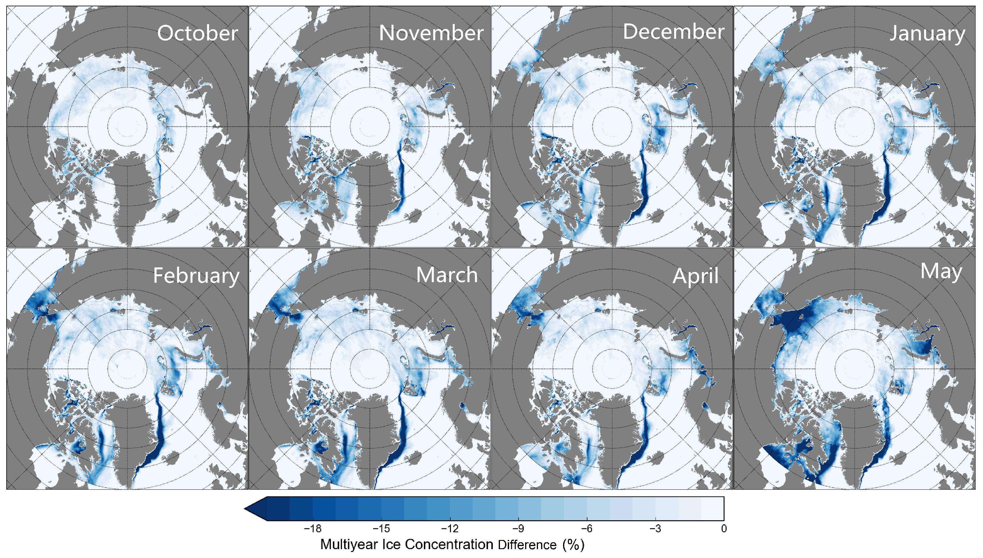
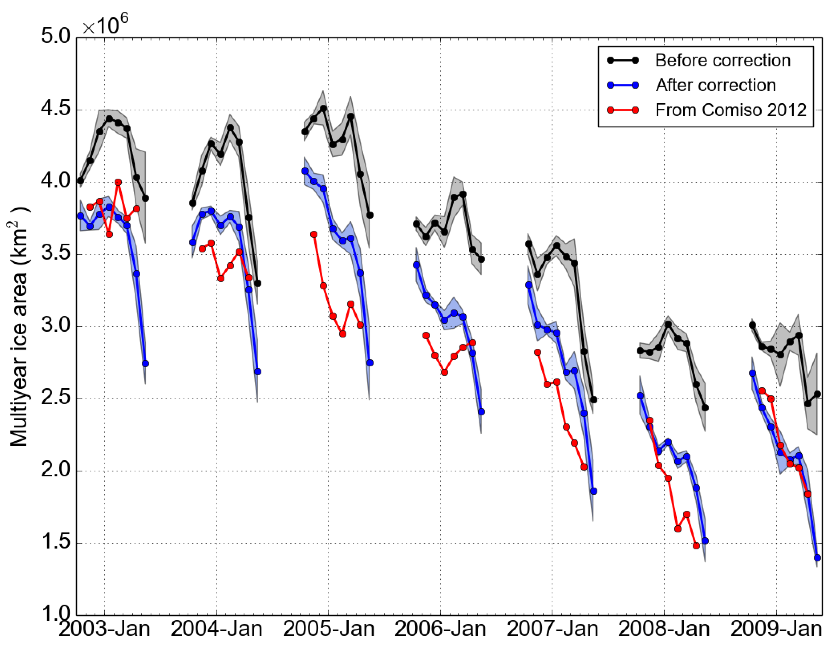
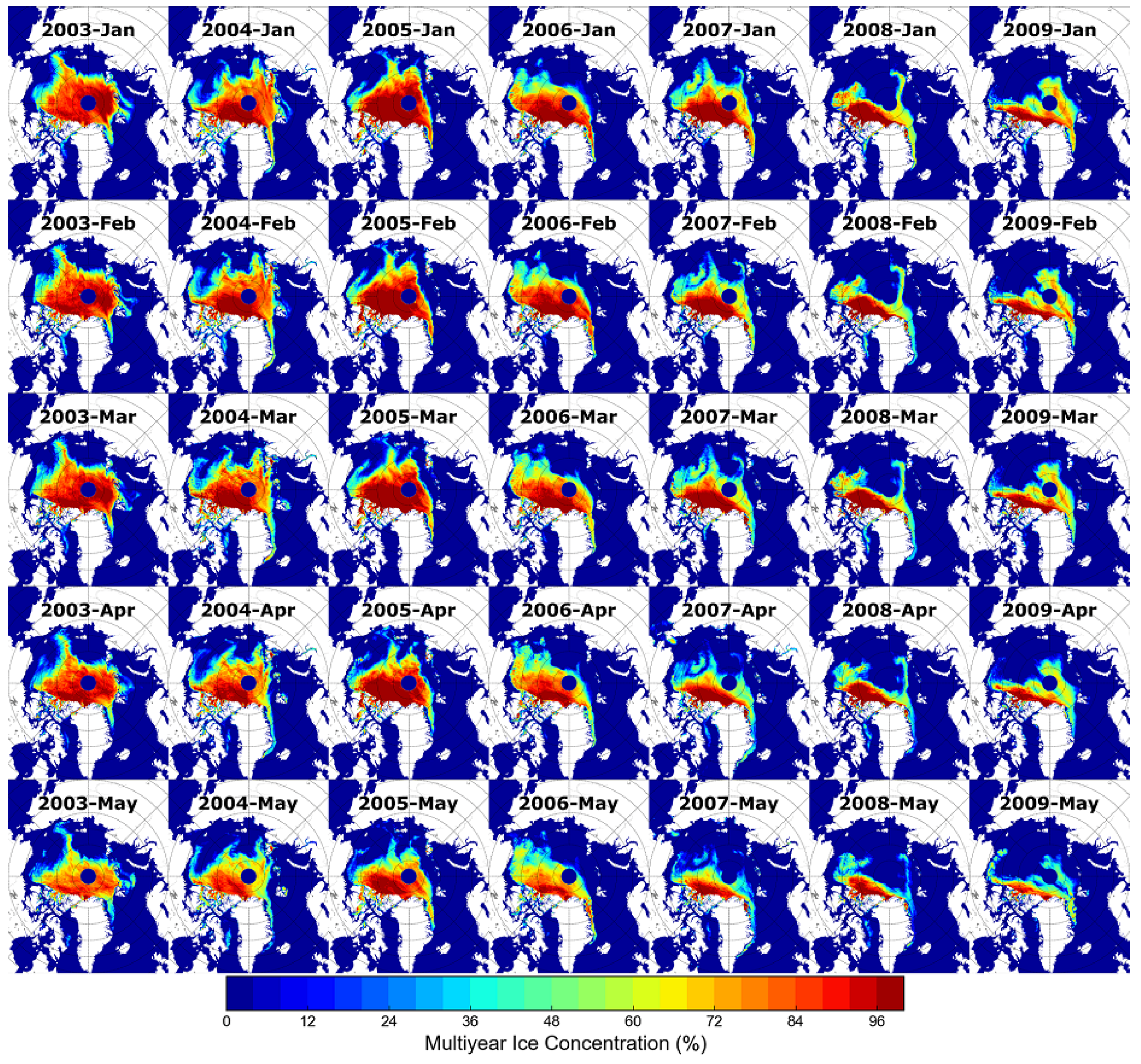
5.3. Inter-Annual Variability over the Entire Arctic

The inter-annual variability of MYI within the Arctic region is presented here as a piece of evidence to support the validation of the correction scheme. Physically speaking, the presence of MYI in the Arctic is governed by two processes, the aging of FYI to second-year ice and the ice export to southern regions through a few known routes. The first process dominates during September-November and the second continues throughout the year. Therefore, it is expected that MYI area in winter increases in the first two or three months, followed by continuous decreases. This criterion can be used to evaluate MYI area product from different methods.

Figure 11 shows the MYI area over the entire (over latitude 60°N) Arctic before and after correction in winter months (October–May) for the period 2002–2009. As described in Section 3, the correction suggested in this study leads to a reduction of MYI, which is obvious in the figure. On average, the reduction is about 5.2 × 10⁵ km² (14.3%) but it exceeds this value in April–May as the warmer weather prompts the conditions of the anomalous snow radiometric signature (see Section 3). The data before correction reveals an increase in the MYI area during October-March before it decreases in April–May. This is unrealistic because the transformation of FYI to MYI is limited to October–November. The correction replaces this trend with a nearly constant value in October–January (about 3.75 × 10⁶ km² in 2003–2004) or a drop in the area starting immediately in October. The latter is a manifestation of the dominant effect of ice export. It should be noted that the correction produces a larger drop in MYI area from October to May. It also results in less fluctuations (i.e., better monotonic decrease) of the MYI area, which is physically more conceivable and a sign of success as explained above. The standard deviations of the estimated MYI area after correction are smaller than the corresponding values before correction in all the winter months except for May. Besides, the correction produces much higher standard deviation in April–May (1.7 × 10⁵ km²) than the rest of the season (0.77 × 10⁵ km²), which can be linked to the higher mobility of the ice cover during the spring months. The results of the MYI retrieval for May should also be treated with more caution, as melting conditions start in parts of the Arctic which hampers reliable MYI retrieval. Potentially, this can lead to an exaggerated drop in MYI area in May.

Comiso [2] studied trends of the Arctic MYI during the winters of 1979–2011 using passive microwave observations. The study detected a rapid rate of decline of MYI area (−17.2% per decade). Part of the results is included in Figure 11 to compare with the results from this study. These two datasets confirm the inter-annual decay of MYI area at nearly the same rate. It should be noted that the results from [2] are not corrected for anomalous brightness temperature. However they are closer to the corrected results than the uncorrected ones from the present study. The underestimation of the [2] except for the winter of 2008–2009 should be attributed to the following two reasons: exclusion of the MYI with concentrations below 30% in [2], and the differences between the two algorithms. The retrieval in [2] is based on solving the linear equations that decompose each observation into components from different surface types, weighted by the concentration of the surface within a resolution cell. A set of monthly varying tie points is used to account for the intra-winter variation of the MYI signature. This is conceptually different than the ECICE method as explained in Section 2.

MYI drifts away from the pack ice in the Arctic to lower latitudes through a few routes but mainly through the Fram Strait located between the Greenland and Svalbard. During winter, the MYI area can only decrease due to ice export and ice deformation, i.e., rafting/ridging. Therefore, it can be expected that on first-order the MYI area variability can be associated with sea ice export through the Fram Strait.

Sea ice export from the Fram Strait is compared to the variability of the MYI decrease in the Arctic Basin during winter. The area export is calculated by multiplying sea ice concentration and sea ice drift along a transect at about 79°N and 20°W–5°E similar to [63], for area but not volume fluxes. The sea ice concentrations are calculated from SSM/I (the Special Sensor Microwave Imager) data using the ASI algorithm [38,64]. For sea ice drift, the 3-daily QuikSCAT-SSM/I dataset from IFREMER/Cersat, Brest, France [65] is used. Both datasets were brought onto the same polar stereographic grid, and gaps in the ice drift dataset were interpolated before the sea ice area flux is calculated. The monthly Fram Strait sea ice export was calculated from the daily area fluxes.

Figure 12 shows the difference in MYI area between November and March (the area in November minus that in March) for the winters from 2002–2003 to 2008–2009, along with the ice area export through the Fram Strait for the same period. The MYI area difference is obtained for the Arctic Basin only by excluding the area between 45°W and 0°W and below 80°N. As investigated in [44], warm air spells leading to misidentification of MYI as FYI occur mostly in September and October. In order to exclude the impact of the temperature correction suggested in [44], the data of these two months are not included in the comparison. Data of April and May are not included also because of their large variations as discussed above.

In the seven winters, the MYI area before correction exhibits increases from November to March except for the winter of 2004–2005. This is physically not realistic because large areas of MYI can be formed during winter and it negates the ice export through the Fram Strait. The correction scheme reverses this wrong trend and produces a decrease of the MYI area which fairly well agrees with the outflow through the Fram Strait, which makes up about 90% of the Arctic sea ice export. It is worth noting that the ice area flux is calculated regardless of ice type but the ice drifting from the central Arctic through the Fram Strait includes a high percentage of MYI. MYI export is the major cause for changes in MYI area during winter time. The only other possible mechanism is sea ice ridging, which also can reduce the MYI area but to a much smaller degree. Therefore some correspondence but no perfect match should be expected between the winter MYI area decrease and the winter Fram Strait ice area export. The two time series (blue and red curves in Figure 12) show good correspondence for several years. For example the above average decrease of MYI area in winter 2004–2005 is also visible in an enhanced ice export. The MYI decrease in winter 2006–2007 is the third highest of the seven-year time series but not very pronounced. The ice export in winter 2006–2007 is even the second lowest of the time series. Both hinting to the loss of MYI in the previous winter was not the major driver for the sea ice minimum in 2007. We consider the much better agreement of the winter MYI area decrease with the Arctic ice export after the correction as another evidence for the improvement, which can be attributed to the present correction scheme.

Figure 13 shows the monthly average MYI concentration maps from January to May for the years from 2003 to 2009. Within each year, the MYI coverage decreased as the freezing season progressed after January. This is mainly due to ice advection and a much less degree because of ridging. For the MYI area decrease from one year to the next, melt across the Beaufort Sea can also be an explanation. Kwok et al. [66] studied the contribution of melt in the Beaufort Sea to the decline of sea ice area. It is found that the net melt area in the Beaufort Sea between 2005 and 2008 accounts for nearly 32% of the net loss of Arctic MYI coverage over the same period. Figure 13 shows two notable decreases of MYI area in January 2006 and January 2008 compared to the same month in the previous years. These should be linked to the findings of the first and second minima of the Arctic ice extent, observed in September 2005 (5.56 × 10⁶ km²; a 0.94% drop relative to 1981–2010 average) and 2007 (4.29 × 10⁶ km²) (National Snow and Ice Data Center, NSIDC, [67]). Please cite it as a new reference This figure confirms the trend established in previous studies (e.g., [68]) that MYI continues to be pushed against northern Greenland, Ellesmere Island and Queen Elizabeth Island, where it is either deformed or advected further southwards through passages in the Canadian Arctic Archipelago.

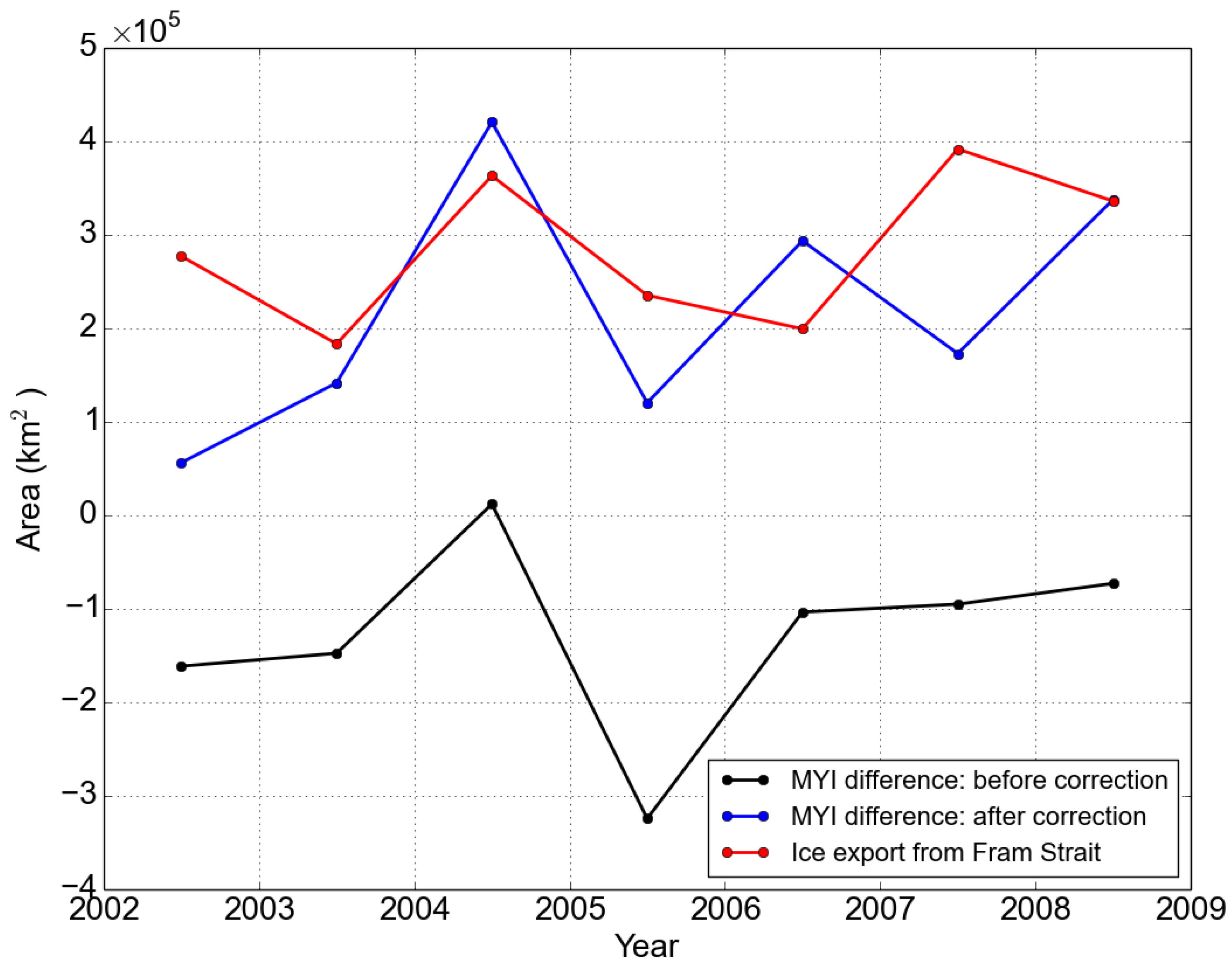
5.4. Regional Sensitivity to the Correction

As mentioned in Section 5.1, the correction incorporates two schemes. The first, which is based on records of atmospheric temperature, is used mainly to correct anomalies observed in September-October [44]. The second, which accounts for snow wetness/metamorphism and employs ice drift data, is the one described in Section 3 and Section 4. Results from the second scheme only are presented in Figure 14. The figure shows maps of the difference between the corrected and uncorrected MYI concentration. Each panel represents the average over the given month using all the available months from October 2002 to May 2009. The regional distribution where the correction scheme is applied can be clearly seen from the figure.

Minor differences are observed in the data of October and to some extent November before the differences become more pronounced in late winter and spring months. The differences are always restricted to the peripheral of the Arctic Basin, where atmospheric temperatures are higher than those in the central Arctic and ice deformation due to waves and storms is more prevalent. These areas usually feature FYI and YI that can be misidentified as MYI when snow conditions lead to anomalous radiometric signature. More differences are found along the ice drift routes in the Greenland Sea and the Baffin Bay. Lower latitudes of the Chukchi Sea and Bering Sea (associated with relatively higher winter temperature) reveal also larger differences after January when the region is covered with thick snow over FYI that will metamorphose under favourable meteorological conditions. The largest differences are observed in May, which marks common dates of pre-melt and melt onset conditions [69], hence extensive snow metamorphism. The dark blue color in the map of May indicates where discrimination between FYI as MYI can be problematic using microwave observations. This is noticeable in the Chukchi Sea, Bering Sea, Kara Sea, as well as the Baffin Bay and Hudson Bay. These areas should be carefully considered when evaluating performances of different MYI retrieval algorithms, which do not work during summer months and already can show degrading performance in May. It should be noted that the false estimate of MYI is common in the Barents Sea between Novaya Zemlya and Svalbard during the entire freezing season, though at a noticeably lower level in May when most of the ice has already melted or drifted away.

6. Conclusions

When the atmospheric temperature approaches the melting point, physical properties of snow on FYI change, triggering anomalous brightness temperatures and backscatters, which deviate from the typical values. These values from FYI become very similar to those from MYI. Deformation and roughening of the ice surface can have a similar effect. These radiometric observations lead to misidentification of FYI as MYI, resulting in erroneous high MYI concentration retrievals. A correction utilizing ice drift records, along with thresholds on the derived parameters from the passive microwave observations, is suggested and applied to the MYI concentration retrieval from ECICE. The correction is applied on the retrieval between October and May for the seven years from 2002 to 2009. The retrieval is preprocessed by another correction suggested in [44] to account for a different radiometric anomaly that leads to misidentification of MYI as FYI.

It is worth mentioning that the corrections presented here and in [44] take the spatial and temporal continuity of MYI into account, which was not considered in the MYI concentration retrieval algorithms.

The correction presented here, which leads to a reduction of the MYI area, is designed to constrain the MYI concentration changes within a plausible contour on a given day, when ice drift data is used to expand the contour of the previous day. On average, the reduction is about 5.2 × 10⁵ km² (14.3%) but it exceeds this value in April–May as warmer weather prompts the conditions of the anomalous snow radiometric signature. In October–March, the MYI area without correction increases, which is physically not realistic. After correction, the MYI area stays fairly constant in October–January or decreases immediately in October. The corrected MYI time series shows a realistic decrease of MYI area during winter, which can be expected as MYI continues to be exported out of the Arctic Basin. The loss in MYI area between November and March is of the same magnitude and shows similar variability as the observed sea ice export through the Fram Strait. The much better agreement of the winter MYI area decrease with the Arctic ice export after the correction gives evidence of the improvement, which is attributed to the present correction scheme.

Maps of the difference between the corrected and uncorrected MYI concentrations show that the difference is most pronounced in months between January and May, and prominent in the peripheral seas of the Arctic. Areas where the differences are larger and atmospheric temperatures are higher, e.g., the Greenland Sea, the Baffin Bay, the Kara Sea, the Chukchi and Bering Seas, should be carefully considered when evaluating performances of different MYI retrieval algorithm.

The comparison with Radarsat-1 SAR images shows that the correction works well by removing unexpected anomalous high MYI concentrations in the peripheral seas of the Arctic except for one case in the Greenland Sea, where assessment of the correction remains crucial because of the possibility of a higher uncertainty of the ice drift product.

To conclude, the correction works well by constraining the MYI concentrations from increasing suddenly and unrealistically in the peripheral seas of the Arctic. It can be applied as a post-processing to all the microwave-based MYI retrieval algorithms, such as the NASA Team algorithm [22,27], the NORSEX algorithm [70], the UMass-AES algorithm [71], and the ECICE algorithm [29]. As warm air spells frequently occur in late winter and spring months and in the peripheral Arctic Seas, it is crucial to consider this situation when retrieving partial ice concentrations. The derived MYI time series after correction is more consistent and fluctuates less, therefore the correction can be important in climatological research and operational applications.

The fundamentally new aspect of the correction suggested here is the insight that instantaneous observations alone of sea ice may lead to ambiguities in determination of the concentration of sea ice types. Instead, the development in time, here of the ice motion, is also crucial for the retrieval. This approach may be applicable to the retrieval of other sea ice parameters, too, especially to sea ice emissivity. In principle, for the retrieval, a forward model combined with an inversion procedure would be preferable, as it has been done over open ocean to retrieve surface and atmospheric parameters for many years [72]. Similar procedures have also been suggested over sea ice (e.g., [73]). However, their results are much less reliable. The reason is that we cannot predict sea ice emissivity at the scale of satellite sensor footprints due to the high horizontal and vertical variability of the sea ice microphysical properties, which are required as input for sea ice emissivity models but are difficult to measure. As long as this flaw persists, the approach forwarded in this paper may be the best possibility to more accurately determine the Arctic multiyear ice concentration, which in turn is required for a more accurate description of the radiative and dynamic processes in the sea ice covered Arctic.

References

1. Cavalieri, D.; Parkinson, C. Arctic sea ice variability and trends, 1979–2010. Cryosphere 2012, 6, 881–889. [Google Scholar] [CrossRef]
2. Comiso, J.C. Large Decadal Decline of the Arctic Multiyear Ice Cover. J. Clim. 2012, 25, 1176–1193. [Google Scholar] [CrossRef]
3. Comiso, J.C.; Parkinson, C.L.; Gersten, R.; Stock, L. Accelerated decline in the Arctic sea ice cover. Geophys. Res. Lett. 2008, 35, L01703. [Google Scholar] [CrossRef]
4. Stroeve, J.; Holland, M.M.; Meier, W.; Scambos, T.; Serreze, M. Arctic sea ice decline: Faster than forecast. Geophys. Res. Lett. 2007, 34, L09501. [Google Scholar] [CrossRef]
5. Comiso, J.C. Abrupt decline in the Arctic winter sea ice cover. Geophys. Res. Lett. 2006, 33, L18504. [Google Scholar] [CrossRef]
6. Comiso, J.C. A rapidly declining perennial sea ice cover in the Arctic. Geophys. Res. Lett. 2002, 29. [Google Scholar] [CrossRef]
7. Johannessen, O.M.; Shalina, E.V.; Miles, M.W. Satellite evidence for an Arctic sea ice cover in transformation. Science 1999, 286, 1937–1939. [Google Scholar] [CrossRef] [PubMed]
8. Kwok, R. Near zero replenishment of the Arctic multiyear sea ice cover at the end of 2005 summer. Geophys. Res. Lett. 2007, 34, L05501. [Google Scholar] [CrossRef]
9. Kwok, R.; Untersteiner, N. The thinning of Arctic sea ice. Phys. Today 2011, 64, 36–41. [Google Scholar] [CrossRef]
10. Perovich, D.K.; Richter-Menge, J.A. Loss of sea ice in the arctic. Ann. Rev. Mar. Sci. 2009, 1, 417–441. [Google Scholar] [CrossRef] [PubMed]
11. Vihma, T. Effects of Arctic Sea Ice Decline on Weather and Climate: A Review. Surv. Geophys. 2014, 35, 1175–1214. [Google Scholar] [CrossRef]
12. Petrie, R.E.; Shaffrey, L.C.; Sutton, R.T. Atmospheric response in summer linked to recent Arctic sea ice loss. Q. J. R. Meteorolog. Soc. 2015, 141, 2070–2076. [Google Scholar] [CrossRef]
13. Kwok, R.; Cunningham, G.; Wensnahan, M.; Rigor, I.; Zwally, H.; Yi, D. Thinning and volume loss of the Arctic Ocean sea ice cover: 2003–2008. J. Geophys. Res. Oceans 2009, 114, C07005. [Google Scholar] [CrossRef]
14. Stroeve, J.C.; Serreze, M.C.; Holland, M.M.; Kay, J.E.; Malanik, J.; Barrett, A.P. The Arctic′s rapidly shrinking sea ice cover: a research synthesis. Clim. Change 2012, 110, 1005–1027. [Google Scholar] [CrossRef]
15. Kwok, R.; Spreen, G.; Pang, S. Arctic sea ice circulation and drift speed: Decadal trends and ocean currents. J. Geophys. Res. Oceans 2013, 118, 2408–2425. [Google Scholar] [CrossRef]
16. Notz, D. The future of ice sheets and sea ice: Between reversible retreat and unstoppable loss. Proc. Natl. Acad. Sci. USA 2009, 106, 20590–20595. [Google Scholar] [CrossRef] [PubMed]
17. Shokr, M.; Dabboor, M. Interannual variability of young ice in the Arctic estimated between 2002 and 2009. IEEE Trans. Geosci. Remote Sens. 2013, 51, 3354–3370. [Google Scholar] [CrossRef]
18. Haas, C.; Howell, S.E. Ice thickness in the Northwest Passage. Geophys. Res. Lett. 2015, 42, 7673–7680. [Google Scholar] [CrossRef]
19. Howell, S.E.; Wohlleben, T.; Dabboor, M.; Derksen, C.; Komarov, A.; Pizzolato, L. Recent changes in the exchange of sea ice between the Arctic Ocean and the Canadian Arctic Archipelago. J. Geophys. Res. Oceans 2013, 118, 3595–3607. [Google Scholar] [CrossRef]
20. Ivanova, N.; Johannessen, O.M.; Pedersen, L.T.; Tonboe, R.T. Retrieval of Arctic sea ice parameters by satellite passive microwave sensors: A comparison of eleven sea ice concentration algorithms. IEEE Trans. Geosci. Remote Sens. 2014, 52, 7233–7246. [Google Scholar] [CrossRef]
21. Cavalieri, D.J.; Gloersen, P.; Campbell, W.J. Determination of sea ice parameters with the Nimbus 7 SMMR. J. Geophys. Res. Atmos. 1984, 89, 5355–5369. [Google Scholar] [CrossRef]
22. Steffen, K.; Schweiger, A. NASA team algorithm for sea ice concentration retrieval from Defense Meteorological Satellite Program special sensor microwave imager: Comparison with Landsat satellite imagery. J. Geophys. Res. Oceans 1991, 96, 21971–21987. [Google Scholar] [CrossRef]
23. Lomax, A.S.; Lubin, D.; Whritner, R.H. The potential for interpreting total and multiyear ice concentrations in SSM/I 85.5 GHz imagery. Remote Sens. Environ. 1995, 54, 13–26. [Google Scholar] [CrossRef]
24. Comiso, J.C.; Cavalieri, D.J.; Parkinson, C.L.; Gloersen, P. Passive microwave algorithms for sea ice concentration: A comparison of two techniques. Remote Sens. Environ. 1997, 60, 357–384. [Google Scholar] [CrossRef]
25. Kwok, R. Annual cycles of multiyear sea ice coverage of the Arctic Ocean: 1999–2003. J. Geophys. Res. Oceans 2004, 109, C11004. [Google Scholar] [CrossRef]
26. Wang, H.; Heygster, G.; Shouzong, H.; Cheng, B. Arctic multiyear ice concentration retrieval based on AMSR-E 89GHz data. Chin. J. Polar Res. 2009, 21, 186–196. [Google Scholar]
27. Ye, Y.; Heygster, G. Towards an Interdisciplinary Approach in Earth System Science: Advances of a Helmholtz Graduate Research School; Chapter Arctic Multiyear Ice Concentration Retrieval from SSM/I Data Using the NASA Team Algorithm with Dynamic Tie Points; Springer International Publishing: Cham, Germany, 2015; pp. 99–108. [Google Scholar]
28. Markus, T.; Cavalieri, D.J. An enhancement of the NASA Team sea ice algorithm. IEEE Trans. Geosci. Remote Sens. 2000, 38, 1387–1398. [Google Scholar] [CrossRef]
29. Shokr, M.; Lambe, A.; Agnew, T. A new algorithm (ECICE) to estimate ice concentration from remote sensing observations: An application to 85-GHz passive microwave data. IEEE Trans. Geosci. Remote Sens. 2008, 46, 4104–4121. [Google Scholar] [CrossRef]
30. Shokr, M.; Agnew, T.A. Validation and potential applications of Environment Canada Ice Concentration Extractor (ECICE) algorithm to Arctic ice by combining AMSR-E and QuikSCAT observations. Remote Sens. Environ. 2013, 128, 315–332. [Google Scholar] [CrossRef]
31. Voss, S.; Heygster, G.; Ezraty, R. Improving sea ice type discrimination by the simultaneous use of SSM/I and scatterometer data. Polar Res. 2003, 22, 35–42. [Google Scholar] [CrossRef]
32. Tschudi, M.; Fowler, C.; Maslanik, J.; Stroeve, J. Tracking the movement and changing surface characteristics of Arctic sea ice. IEEE J. Selected Topics Appl. Earth Obs. Remote Sens. 2010, 3, 536–540. [Google Scholar] [CrossRef]
33. Fowler, C.; Emery, W.; Tschudi, M. Polar Pathfinder Daily 25 km EASE-grid Sea Ice Motion Vectors; Version 2; NASA National Snow and Ice Data Center Distributed Active Archive Center: Boulder, CO, USA, 2013. [Google Scholar]
34. Hoffman, R.N.; Leidner, S.M. An introduction to the near-real-time QuikSCAT data. Weather Forecast. 2005, 20, 476–493. [Google Scholar] [CrossRef]
35. Comiso, J.C.; Cavalieri, D.J.; Markus, T. Sea ice concentration, ice temperature, and snow depth using AMSR-E data. IEEE Trans. Geosci. Remote Sens. 2003, 41, 243–252. [Google Scholar] [CrossRef]
36. Meier, W.N.; Dai, M. High-resolution sea-ice motions from AMSR-E imagery. Ann. Glaciol. 2006, 44, 352–356. [Google Scholar] [CrossRef]
37. Comiso, J.C.; Parkinson, C.L. Arctic sea ice parameters from AMSR-E data using two techniques and comparisons with sea ice from SSM/I. J. Geophys. Res. Oceans 2008, 113, C02S05. [Google Scholar] [CrossRef]
38. Spreen, G.; Kaleschke, L.; Heygster, G. Sea ice remote sensing using AMSR-E 89-GHz channels. J. Geophys. Res. Oceans 2008, 113, C02S03. [Google Scholar] [CrossRef]
39. Early, D.S.; Long, D.G. Image reconstruction and enhanced resolution imaging from irregular samples. IEEE Trans. Geosci. Remote Sens. 2001, 39, 291–302. [Google Scholar] [CrossRef]
40. Long, D.G.; Daum, D.L. Spatial resolution enhancement of SSM/I data. IEEE Trans. Geosci. Remote Sens. 1998, 36, 407–417. [Google Scholar] [CrossRef]
41. Long, D.G.; Hardin, P.J.; Whiting, P.T. Resolution enhancement of spaceborne scatterometer data. IEEE Trans. Geosci. Remote Sens. 1993, 31, 700–715. [Google Scholar] [CrossRef]
42. Isaaks, E.H.; Srivastava, R.M. An Introduction to Applied Geostatistics; Oxford University Press: New York, NY, USA, 1989; p. 561. [Google Scholar]
43. Tonboe, R.; Andersen, S.; Toudal, L. Anomalous Winter Sea Ice Backscatter and Brightness Temperatures; Danish Meteorological Institute Technical Report 03-13; Danish Meteorological Institute: Copenhagen, Denmark, September 2003; pp. 3–13. [Google Scholar]
44. Ye, Y.; Heygster, G.; Shokr, M. Improving multiyear ice concentration estimates with reanalysis air temperatures. IEEE Trans. Geosci. Remote Sens. 2016, 54, 2602–2614. [Google Scholar] [CrossRef]
45. Dee, D.; Uppala, S.; Simmons, A.; Berrisford, P.; Poli, P.; Kobayashi, S.; Andrae, U.; Balmaseda, M.; Balsamo, G.; Bauer, P.; et al. The ERA-Interim reanalysis: Configuration and performance of the data assimilation system. Q. J. R. Meteorolog. Soc. 2011, 137, 553–597. [Google Scholar] [CrossRef]
46. Fuhrhop, R.; Grenfell, T.C.; Heygster, G.; Johnsen, K.P.; Schlüssel, P.; Schrader, M.; Simmer, C. A combined radiative transfer model for sea ice, open ocean, and atmosphere. Radio Sci. 1998, 33, 303–316. [Google Scholar] [CrossRef] [Green Version]
47. Shokr, M.; Sinha, N. Sea Ice: Physics and Remote Sensing; John Wiley & Sons: Hoboken, NJ, USA, 2015. [Google Scholar]
48. Comiso, J.; Ackley, S.; Gordon, A. Antarctic sea ice microwave signatures and their correlation with in situ ice observations. J. Geophys. Res. Oceans 1984, 89, 662–672. [Google Scholar] [CrossRef]
49. Shokr, M.; Asmus, K.; Agnew, T.A. Microwave emission observations from artificial thin sea ice: The ice-tank experiment. IEEE Trans. Geosci. Remote Sens. 2009, 47, 325–338. [Google Scholar] [CrossRef]
50. Anderson, M.R. Determination of a melt-onset date for Arctic sea-ice regions using passive-microwave data. Ann. Glaciol. 1997, 25, 382–387. [Google Scholar]
51. Drobot, S.D.; Anderson, M.R. An improved method for determining snowmelt onset dates over Arctic sea ice using scanning multichannel microwave radiometer and Special Sensor Microwave/Imager data. J. Geophys. Res. Atmos. 2001, 106, 24033–24049. [Google Scholar] [CrossRef]
52. Koskinen, J.; Pulliainen, J.; Hallikainen, M. Effect of snow wetness to C-band backscatter-a modeling approach. In Geoscience and Remote Sensing Symposium, 2000, Proceeding of the IEEE 2000 International IGARSS, 24–28 July 2000; IEEE: Honolulu, HI, USA; Volume 4, pp. 1754–1756.
53. Barber, D.G. Microwave remote sensing, sea ice and Arctic climate. Phys. Can. 2005, 61, 105–111. [Google Scholar]
54. Du, J.; Shi, J.; Rott, H. Comparison between a multi-scattering and multi-layer snow scattering model and its parameterized snow backscattering model. Remote Sens. Environ. 2010, 114, 1089–1098. [Google Scholar] [CrossRef]
55. Sumata, H.; Lavergne, T.; Girard-Ardhuin, F.; Kimura, N.; Tschudi, M.A.; Kauker, F.; Karcher, M.; Gerdes, R. An intercomparison of Arctic ice drift products to deduce uncertainty estimates. J. Geophys. Res. Oceans 2014, 119, 4887–4921. [Google Scholar] [CrossRef] [Green Version]
56. Sumata, H.; Kwok, R.; Gerdes, R.; Kauker, F.; Karcher, M. Uncertainty of Arctic summer ice drift assessed by high-resolution SAR data. J. Geophys. Res. Oceans 2015, 120, 5285–5301. [Google Scholar] [CrossRef]
57. Anderson, M.R. The onset of spring melt in first-year ice regions of the Arctic as determined from scanning multichannel microwave radiometer data for 1979 and 1980. J. Geophys. Res. Oceans 1987, 92, 13153–13163. [Google Scholar] [CrossRef]
58. Mundy, C.; Barber, D. On the relationship between spatial patterns of sea-ice type and the mechanisms which create and maintain the North Water (NOW) polynya. Atmosphere-Ocean 2001, 39, 327–341. [Google Scholar] [CrossRef]
59. Barber, D.G.; Massom, R.A. The role of sea ice in Arctic and Antarctic polynyas. Elsevier Oceanogr. Ser. 2007, 74, 1–54. [Google Scholar]
60. Hilmer, M.; Harder, M.; Lemke, P. Sea ice transport: A highly variable link between Arctic and North Atlantic. Geophys. Res. Lett. 1998, 25, 3359–3362. [Google Scholar] [CrossRef]
61. Rigor, I.G.; Wallace, J.M.; Colony, R.L. Response of sea ice to the Arctic Oscillation. J. Clim. 2002, 15, 2648–2663. [Google Scholar] [CrossRef]
62. Kimura, N.; Nishimura, A.; Tanaka, Y.; Yamaguchi, H. Influence of winter sea-ice motion on summer ice cover in the Arctic. Polar Res. 2013, 32, 20193. [Google Scholar] [CrossRef]
63. Spreen, G.; Kern, S.; Stammer, D.; Hansen, E. Fram Strait sea ice volume export estimated between 2003 and 2008 from satellite data. Geophys. Res. Lett. 2009, 36, L19502. [Google Scholar] [CrossRef]
64. Kaleschke, L.; Lüpkes, C.; Vihma, T.; Haarpaintner, J.; Bochert, A.; Hartmann, J.; Heygster, G. SSM/I sea ice remote sensing for mesoscale ocean-atmosphere interaction analysis. Can. J. Remote Sens. 2001, 27, 526–537. [Google Scholar] [CrossRef]
65. Girard-Ardhuin, F.; Ezraty, R. Enhanced Arctic sea ice drift estimation merging radiometer and scatterometer data. IEEE Trans. Geosci. Remote Sens. 2012, 50, 2639–2648. [Google Scholar] [CrossRef]
66. Kwok, R.; Cunningham, G. Contribution of melt in the Beaufort Sea to the decline in Arctic multiyear sea ice coverage: 1993–2009. Geophys. Res. Lett. 2010, 37, L20501. [Google Scholar] [CrossRef]
67. NSIDC. State of the Cryosphere: Sea Ice. Available online: https://nsidc.org/cryosphere/sotc/sea_ice.html (accessed on 19 April 2016).
68. Kwok, R. Exchange of sea ice between the Arctic Ocean and the Canadian Arctic Archipelago. Geophys. Res. Lett. 2006, 33, L16501. [Google Scholar] [CrossRef]
69. Markus, T.; Stroeve, J.C.; Miller, J. Recent changes in Arctic sea ice melt onset, freezeup, and melt season length. J. Geophys. Res. Oceans 2009, 114, C12024. [Google Scholar] [CrossRef]
70. Svendsen, E.; Kloster, K.; Farrelly, B.; Johannessen, O.; Johannessen, J.; Campbell, W.; Gloersen, P.; Cavalieri, D.; Mätzler, C. Norwegian remote sensing experiment: Evaluation of the nimbus 7 scanning multichannel microwave radiometer for sea ice research. J. Geophys. Res. Oceans 1983, 88, 2781–2791. [Google Scholar] [CrossRef]
71. Swift, C.; Fedor, L.; Ramseier, R. An algorithm to measure sea ice concentration with microwave radiometers. J. Geophys. Res. Oceans 1985, 90, 1087–1099. [Google Scholar] [CrossRef]
72. Wentz, F.J.; Meissner, T. AMSR Ocean Algorithm, Algorithm Theoretical Basis Document (ATBD); Version 2; RSS Tech. Proposal 121599A-1; Remote Sensing Systems: Santa Rosa, CA, USA, 2000. [Google Scholar]
73. Melsheimer, C.; Heygster, G.; Mathew, N.; Pedersen, L.T. Retrieval of sea ice emissivity and integrated retrieval of surface and atmospheric parameters over the Arctic from AMSR-E data. J. Remote Sens. Soc. Jpn. 2009, 29, 236–241. [Google Scholar]
Figure 1. (a) Surface air temperature from the ERA-Interim reanalysis [45]; (b) multiyear ice concentration; and (c) first-year ice concentration retrieved from Environmental Canada Ice Concentration Extractor (ECICE) from 6 April to 13 May 2003. The red stars indicate the sample region that will be mentioned in Figure 2.
Remotesensing 08 00397 g001
Figure 2. Averaged multiyear (CMYI), first-year ice concentration (CFYI) and total sea ice concentration (CTOT), surface air temperature (T), brightness temperature (Tb37h, Tb37v and Tb19h), backscatter ( σ h h 0 and σ v v 0 ) and horizontal range (HR = Tb19hTb37h) of a selected region in the Barents Sea (latitude: 76.75°–77°N, longitude: 29°–30°E, as the red stars shown in Figure 1a) from October 2002 to May 2003. The five vertical blue lines correspond to the five events of sudden increases in MYI concentration as described in the text.
Remotesensing 08 00397 g002
Figure 3. Flowchart of the correction procedure. (a) The originally-estimated MYI domain; (b) expansion accordingly to ice drift; (c) regions outside and inside the expanded MYI domain.
Remotesensing 08 00397 g003
Figure 4. Probability distribution of ΔCMYI for the non-anomalies and anomalies from 2002 to 2009.
Remotesensing 08 00397 g004
Figure 5. Probability distribution of daily changes of brightness temperature at vertical polarized 37 GHz (ΔTb37h) for the non-anomalies and anomalies from 2002 to 2009.
Remotesensing 08 00397 g005
Figure 6. Multiyear ice concentrations from the ECICE algorithm (top) and those after the correction (bottom) on selected days in April–May 2003.
Remotesensing 08 00397 g006
Figure 7. (a) MYI concentration map from ECICE for 2 April 2003 before correction; (b) the MYI concentration map after correction; (c) the Radarsat-1 image.
Remotesensing 08 00397 g007
Figure 8. (a) MYI concentration map from ECICE for 6 May 2003 before correction, with the frame of Radarsat-1 image overlaid; (b) the same frame with the MYI concentration map after correction; (c) the Radarsat-1 image. The red box indicates frame of the Radarsat-1 image.
Remotesensing 08 00397 g008
Figure 9. (a) MYI concentration map from ECICE for 14 May 2003 before correction, with the frame of Radarsat-1 image overlaid; (b) MYI concentration map after correction, with the same frame of the Radarsat-1 image; (c) the Radarsat-1 image. The red box indicates frame of the Radarsat-1 image.
Remotesensing 08 00397 g009
Figure 10. (a) MYI concentration map from ECICE for 20 May 2003 before correction, with the frame of Radarsat-1 image overlaid; (b) MYI concentration map after correction, with the same frame of the Radarsat-1 image; (c) the Radarsat-1 image. The red box indicates frame of the Radarsat-1 image.
Remotesensing 08 00397 g010
Figure 11. Monthly averaged Arctic multiyear ice area before and after correction in winters (October–May) from 2002 to 2009. The red line represents the monthly averaged multiyear ice area adapted from [2] (November–April). © American Meteorological Society. Used with permission. The gray and light blue areas indicate the standard deviation of the multiyear ice area of each month.
Remotesensing 08 00397 g011
Figure 12. The MYI area difference between November and March (the area in November minus that in March) and the ice export through the Fram Strait from 2002–2003 to 2008–2009. The black and blue lines depict the decreases of the MYI area before and after correction, respectively. The calculation of MYI area excludes the Greenland Sea south of the Fram Strait (latitude: 60°N–80°N, longitude: 45°W–0°W).
Remotesensing 08 00397 g012
Figure 13. Monthly average concentration of multiyear ice after correction for January–May of the years 2003–2009.
Remotesensing 08 00397 g013
Figure 14. Corrected minus uncorrected MYI concentration maps resulting from the presented correction scheme. Data for each month are averaged over the winter months available from 2002–2003 to 2008–2009.
Remotesensing 08 00397 g014