Abstract
This work introduces a new classification method in the remote sensing domain, suitably adapted to dealing with the challenges posed by the big data processing and analytics framework. The method is based on symbolic learning techniques, and it is designed to work in complex and information-abundant environments, where relationships among different data layers are assessed in model-free and computationally-effective modalities. The two main stages of the method are the data reduction-sequencing and the association analysis. The former refers to data representation; the latter searches for systematic relationships between data instances derived from images and spatial information encoded in supervisory signals. Subsequently, a new measure named the evidence-based normalized differential index, inspired by the probability-based family of objective interestingness measures, evaluates these associations. Additional information about the computational complexity of the classification algorithm and some critical remarks are briefly introduced. An application of land cover mapping where the input image features are morphological and radiometric descriptors demonstrates the capacity of the method; in this instructive application, a subset of eight classes from the Corine Land Cover is used as the reference source to guide the training phase.
1. Introduction
Since the 1970s, Earth observation or remote sensing (RS) data have been acknowledged as relevant sources of information for a long list of disciplines, including (but not limited to) Earth sciences and geology, environmental sciences, water and coastal management, territorial planning, forestry and agriculture [1,2]. Nowadays, digital Earth observation data and geo-spatial information are considered key assets for understanding the processes shaping the planet Earth [3,4,5]. They can provide fundamental inputs needed for improving global evidence-based decision-making processes, as the ones envisaged in the United Nations Sustainable Development Goals (https://sustainabledevelopment.un.org/sdgs), the Post-2015 Framework for Disaster Risk Reduction (http://www.unisdr.org/we/coordinate/hfa-post2015) and the United Nations Framework Convention on Climate Change (http://newsroom.unfccc.int/).
In our current age, data are abundant, exponentially growing in volume, but only partially structured and harmonized. Generated by different agents and serving diverse objectives over time, the accumulated data compose a rich source of information, yet are difficult to effectively explore and analyze globally. Furthermore, the increasing need to collect new data establishes advanced standards regarding the capacity to organize collective volunteer efforts in geographical information gathering [6] and the capacity to design and operate new automatic satellite sensors and platforms improving the spatial, spectral, and temporal resolution of the available remotely-sensed data. In 2008, the U.S. Geological Survey (USGS) released for free to the public its Landsat archive, historical records of Earth observation technology dating back to the 1970s [5,7]; this progression dramatically increases the scale detail and the amount of remote sensing data available for scientific purposes. Moreover, the EU Copernicus space program, started in 2014, is expected to increase the global open and free data collection capacity even more by some orders of magnitude [8].
As a corollary of the above trend, and given the fact that the planet surface is of finite dimensions, a general increase of spatial information redundancy can be expected: nowadays, the chance to find alternative and only partially-harmonized descriptions of the same piece of land made by different geo-spatial information products at different scale, time and thematic technical specifications is much higher than in the very recent past.
Furthermore, our capacity to process and extract significant global information from this exponentially-increasing volume and detail of an only partially-structured and rapidly-changing mass of data is not developing with the same rapidity and effectiveness [9]. The standard causal-deterministic remote sensing data classification models require large amounts of human resources (data experts, domain experts) dedicated to tune, test and adapt the image information extraction models to the specific and rapidly-changing set of data, sensors and target classes. Supervised data classification and machine learning techniques can contribute to mitigating some of these issues by the automatic generation of the inferential models linking the image data with the high abstraction information required by the analytical tasks. However, today’s state of the art machine learning techniques employed in remote sensing applications show severe drawbacks in scenarios where large training sets are used together with large input data. These algorithms have been designed and tested on small to medium data instances (if compared to fine-scale global RS data scenarios) with a moderate to large number of attributes or features and are difficult to scale to geo-spatial big data machine learning problems [10]. These drawbacks are largely amplified in the case of complex and ill-defined target classes’ analytics and in the case of partially-inconsistent, global fine-scale data scenarios.
This manuscript introduces in the remote sensing domain a new generic supervised classification framework that may contribute to solving geo-spatial big data problems. It is based on symbolic machine learning (SML) techniques. As introduced here, the SML consists of two basic processes, namely: (i) input image data reduction sequencing; and (ii) association analysis. During the sequencing stage, the input data are reduced to a set of sequences represented in a symbolic, compact and multidimensionally-sparse mode. The subsequent association analysis stage is used as an automatic inferential engine constructing the rules that are associating the data sequences with a given high-abstraction information layer (the terms reference set, supervisory signal and high-abstraction information layer are used with the same meaning to denote the class set). In the SML name, the term symbolic refers to the fact that the input data are represented by a finite set of symbols, the alphabet of sequences. The term machine learning is used in the general sense introduced in computer science as the field of study that gives computers the ability to learn without being explicitly programmed [11].
The SML framework shows some analogies with data analytics tools already developed and largely applied in other disciplines, such as the genetic association techniques. The association rules in genes (or genetic association) are extensively used in bio-informatics to reveal biologically-relevant associations between different genes or between environmental effects and gene expression [12,13,14,15]. By analogy with the genetic association applied in bio-informatics, the SML association classifier searches for relevant, systematic relationships between sequenced image data instances and supervisory (spatial) information encoded in selected reference sets.
So far, these paradigms have been very rarely applied in the remote sensing community that is dominated by continuous numeric representation of the input signal, which is typically postulated by physical causal-explanatory paradigms [9,16,17].
From the use domain perspective, the SML supervised approach has been formulated as a contribution to tackle the challenges posed by the geo-spatial big data processing and analytics framework [9,16,17]. In this new approach, analogously as argued by [18], causal deterministic models are largely complemented by data-driven inductive inferential reasoning. Moreover, the whole data volume (samples = all available data) is typically used for making the inferences.
This is in contrast to other approaches focusing on the search of laws (or continuous functions in the model-fitting perspective) explaining the relationships among a few carefully-sampled points in the same data universe. In the SML, the goal is the identification of the association rules among parts of comprehensive data series that fully describe the whole universe.
Our goal herein is limited to firstly introduce the SML classifier and then to provide some didactic use examples, helping the reader to understand the basic features of the new general supervised classification framework. The purpose of the manuscript is not to present an application of remote sensing data classification aiming to detect specific land use or land cover classes using specific data as the input. Furthermore, the purpose is not to benchmark or compare the SML with respect to other known supervised classification methods. These points related to the application and benchmarking of SML have been developed in other publications presenting experiments of the automatic recognition of built-up areas from satellite imagery. In [19], SML classifiers are tested in the frame of the Global Human Settlement Layer (GHSL) production workflow. In that experiment, more than 30,000 individual Landsat satellite scenes have been automatically classified using SML for the discrimination of the land vs. water and built-up vs. not built-up target classes. The experiment included satellite data collected by the Landsat platform in the past 40 years with MSS, ETM, and ETM+ sensors, producing data with different spectral characteristics and spatial resolutions of 75 m, 30 m and 15 m. According to the quality tests developed in that experiment, the discrimination of the built-up class in the GHSL product is superior to any other global product available today and generated exclusively by automatic classification techniques. In [20], the SML techniques are tested for the update of the GHSL using Sentinel satellite data input. Finally, in [16], the SML was benchmarked with other well-known parametric and non-parametric classifiers as regards the capacity to discriminate ill-defined information in a controlled experiment connoted by constant input and test data, but considering three scenarios of increasing noise modifying the supervisory signals. According to these experiments, at the parity of data conditions (same input image features and same quality or same noise level of the reference set), the SML approach was generally outperforming both parametric and non-parametric classifiers. For example, considering the average performance of all of the tests elaborated, in terms of informedness (average ± standard deviation), the SML classifier achieved the highest result (0.6098 ± 0.0567). Other classifiers attained inferior average performance (e.g., maximum likelihood: 0.5842 ± 0.0252; support vector machine: 0.5588 ± 0.0678; and random forest: 0.4451 ± 0.1046). For a detailed description of the obtained results, the reader can refer to [16]. Moreover, as related to non-parametric methods, the SML achieved this performance with a computational cost decreased by one to two orders of magnitude.
The remainder of the paper is organized as follows: The basic components of the new symbolic machine learning approach are presented in Section 2. The adopted data reduction-sequencing procedure is detailed in Section 2.1. Section 2.2 introduces the stage of association analysis based on the evidence-based normalized differential index (ENDI). A computational complexity analysis of the algorithmic modules is presented in Section 2.3. Section 3 contains an application of the SML in a specific showcase using multi-spectral Spot 5 data pan-sharpened at a spatial resolution of 2.5 m; as already remarked above, the purpose of these examples is purely didactic in order to show an example of the use of the general SML framework. The data and the target classes used in the experiments are largely arbitrary and selected for didactic purposes: they are not representative of all of the applications that can be developed by the use of the SML classifier. Discussions and conclusions are included in the last Section 4.
2. Basic Components
The method is based on the concept of the empirical multidimensional histogram. Briefly, associations among class labels and tuples of features are defined; feature values have been derived from the grouping/binning of the multidimensional histogram that describes the data under consideration. Then, a normalized measure scores these tuples according to the number of their occurrences in each class. The analysis of the cumulative distribution of the estimated scores results, at the end, in their reclassification. Contiguous concepts have been used in the past, such as the histogram distance index (HDI) [21] and the ‘wave hedges’ [22,23]; more recently, in [24], a similar approach has been employed for the objective evaluation of the information merit in the case of input imagery provided by different sensor platforms.
The SML schema is based on two relatively independent steps:
- Reduce the data instances to a symbolic representation;
- Evaluate the association between the symbolic data instances subdivided into two parts: X (input data) and Y (known class memberships).
The first step can also be called data reduction, and it is mostly required when the input data have a quantitative nature; typically, it involves a grouping/aggregation technique. The second step regards the application of a frequency-based supervised classification. As already mentioned, the two steps are relatively independent: different techniques can be chained in the two components.
Figure 1 shows the specific implementation of an SML classifier as proposed in this manuscript. The features (attributes; in our context, the terms attribute and feature are used interchangeably) of the input dataset are all descriptors of the spatial samples. The pre-processing stage for data reduction consists of three main phases. The first one implies generating a taxonomy (in the case of numerical values, this process usually takes the form of a quantization or discretization); in the second, data sequences are constructed; in the last one, the unique sequences are identified, and their frequencies of occurrence are calculated (frequency analysis). The last action is equivalent to the determination of the support set. If the input data have a symbolic nature, they can be used directly in the association analysis stage. Optionally, taxonomies in the form of recoding tables can be applied on the symbolic data input depending on knowledge-driven reasoning. For example, integrating a specific already available land cover class as the input of a given image classification workflow could be useful.
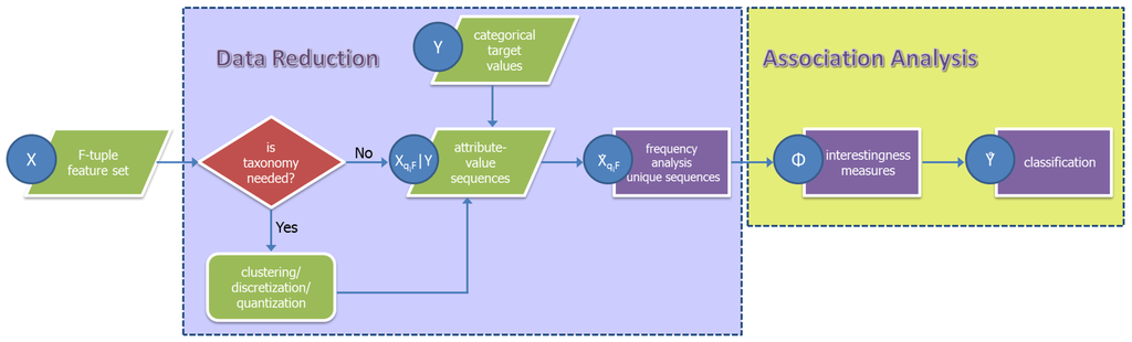
Figure 1.
The general workflow of the symbolic machine learning (SML) classifier.
Remote sensing data are digitized by a process of sampling and quantization of the electro-magnetic energy that is detected by a remote sensor. Usually, these data are available as quasi-continuous numeric values quantized in a given number of levels. Some sensors can collect the information about the energy reflected/emitted by targets in different wavelengths. Consequently, they can produce a string of values associated with each sample (pixel). Moreover, some second-order features can be extracted from the pixel values. Band ratios or combinations implemented in the spectral domain or textural and morphological filtering applied in the spatial domain are typical examples of image transformations in remote sensing. Finally, all of these data may have a multi-temporal nature, producing remote sensing data cubes (an approach for analyzing and visualizing massive datasets used, for instance, by Geoscience Australia (Australian Geoscience Data Cube project http://www.ga.gov.au/about/what-we-do/projects/earth-observation-and-satellite-imagery/australian-geoscience-data-cube) and Google Earth Engine (platform for environmental data analysis https://earthengine.google.com/). All of these features may contribute to the formation of attribute-value sequences and used as input to the SML classifier.
The results of the input data reduction stage, that is the attribute-value sequences , are the antecedent of the following association analysis stage. The consequent in this stage is constituted by data originating from available high-abstraction semantic layers Y. In the typical use scenarios of the SML classifier, Y are proxies of the target categorical information describing the whole data universe under analysis or a large portion of it. For example, they may include land cover data approximating thematically and/or, in the space-time domains, the information to be extracted from the satellite data. Finally, the output of the association analysis is the Φ values given by an interestingness measure; these values are mapped to the single spatial sample (pixel) and used as the decision criterion translating the feature space into the final classification output.
2.1. Data Reduction Sequencing
Numerous methods are available in literature to approach the issues of data reduction, cluster analysis and taxonomy. It is a main task of exploratory data mining, which has appeared in many fields, including remote sensing data analysis, information retrieval and bio-informatics. An extensive introduction and overview to the topic can be found in [25,26].
In this work, the approach of data quantization followed by data sequencing has been chosen. Two main criteria were used to select the proposed data quantization sequencing method. The first criterion comes from the exigency of an objective method, as much as possible independent from assumptions about specific statistical distributions of the input data. This is important in real big remote sensing data scenarios (rBrsDs), because just the analysis of the statistical distribution of specific input data volumes may become computationally very expensive or even prohibitive. This is especially true in rapidly-changing and highly heterogeneous rBrsDs, including continuous streams of image data, which would force the application of ad hoc data reduction approaches. The second criterion is linked to the necessity of adopting a sparse representation of the input data features. Such coding allows the compression of the feature space and increases the computational efficiency in rBrsDs. Recently, in the computer vision community, such representations have been successfully proposed to solve image compression, pattern recognition and image classification tasks: see, for example, [27,28,29,30].
Let be a dataset with spatial samples or pixels and F features or descriptors. Let be a two-dimensional data matrix, , with F expressing the number of used features and . Let be the set of all of the unique data instances of X, having as cardinality ; this magnitude depends on the specific number of symbols used to encode the values and on the number of features F. The average support of can be estimated as:
The influences both the computational and generalization performance of the classifier. Too small of a may lead to over-fitting issues at the successive phase of association analysis. Thus, very often, a re-discretization of x values must be considered in order to keep this issue under control.
Several quantization or discretization methods, including uniform, adaptive and statistical approaches, may be found in the literature as reviewed by [31]. They are all compatible with the general SML framework. In the application presented later on, a uniform quantization approach was implemented, with the quantized data instances defined as follows:
with and . Accordingly, the respective quantized unique data sequences are denoted by . The justification of this choice relies on the fact that it is the computationally least expensive and the most objective method, being independent from the specific statistical data distributions found in the different datasets under processing. The number of eligible symbols per each descriptor is derived by the combination of the raw digital number encoding the specific data D and the quantization parameter .
2.2. Association Analysis
Let be a set of distinct attributes. For any two disjoint attribute-value subsets {X} and {Y} of A, the patterns of the form X → Y are called association rules, where . The attribute-value sets X and Y are called the antecedent and consequent of the association rule, respectively. In the associative classification (AC) framework started by [32], the class association rules are the association rules with a class label attribute as the only consequent ( and , where C is the attribute set containing the class labels).
The proposed method consists of using AC to quantify the association X → Y between multi-attribute data sequences ( in our case) and the available high-abstraction semantic layers Y, using a measure inspired by probability-based objective interestingness measures. The objective measures are those that are not application-specific or user-specific and depend only on the data.
A large set of interestingness measures exists in literature: extensive reviews can be found in [33] and [34]. In this manuscript, a new measure with the name of evidence-based normalized differential index (ENDI) is introduced. It is a generalization of a measure from the confidence family to the case in which a set of positive/negative not-mutually-exclusive examples is provided. The main properties of this index that make it a sound solution in the proposed framework are the following: (1) it is an objective measure; (2) it is algorithmically fast; (3) it is a descriptive measure that does not vary with the cardinality expansion; and (4) it belongs to the measures of deviation from equilibrium [35] taking a fixed value with equilibrium (equiprobability, equal number of positive and negative examples), a necessary property for applications that involve decision- or prediction-making about the consequent. Three variations of the ENDI measure () are proposed herein: they are named , and .
The ENDI confidence measure of the (antecedent) data instances , provided the positive and negative (consequent) data instances, is defined as follows:
where and are the frequencies of the joint occurrences among X (antecedent) data instances and the positive and negative Y (consequent) reference instances, respectively. If only one mutually-exclusive binary training set is provided, the index can be reduced to the measure known as the Charade/Ganascia index proposed by [36] or descriptive confirmed-confidence, as renamed by [37]. The ENDI confidence measure is analogously defined as by substituting the frequencies and with the empirical probabilities and calculated as and , with , denoting, respectively, the numerosity of the positive and negative training samples. The ENDI confidence measure is defined as the median decision between the and the indices, .
With the balanced distribution of the target class (foreground information to be detected in the image data) and its inverse (the background), the different formulations of the , and indices will produce the same or very similar results. They will diverge for increasing unbalance on the classes’ appearance. In particular, assuming the target class referring to the foreground information is very rare in the specific data under analysis, the index will provide a very conservative decision function, minimizing commission error, while on the opposite side, the index will provide a very optimistic decision function, minimizing the omission error. The index provides an intermediate solution of compromise in the case of an unknown prior distribution of the target class.
2.3. Computational Complexity
In this section, m denotes the number of data instances/examples/observations, n the number of features/dimensions/variables, v the number of distinct values per variable, (for simplification reasons, we assume and ) and the number of classes. The total time complexity for the SML training is composed of: (1) the taxonomy of the dataset values; and (2) the data frequencies’ computation, giving a cost of . The brute-force approach yields a worst-case upper bound of order . However, in satellite imagery, the practical dynamic range is reaching the level of 16 bits at most; in addition and after the taxonomy application, the range of values can be reduced considerably. Exploiting techniques like bit arrays and hash tables, a pragmatic time complexity can reach the order of , with integer v ≤ 65,535. In terms of memory requirements, the worst case scenario is realized when all of the data instances of the initial dataset are unique, ; the extra structure of size contains the occurrences of every unique data instance observed in each of the classes. According to the previous analysis, the pragmatic space complexity is . At the classification stage, a new n-datum receives a score based on its frequency in every class and gets a class label depending on the threshold applied over the score, resulting in ; there is also an additional cost to match the n-datum with an element of the unique data instances matrix, a cost that becomes in the case of hashing; the space complexity remains the same, .
2.4. Critical Remarks
There is a sharp difference in the way SML and other formal machine learning techniques are operating. With the standard classifiers, there is a small, representative training set over which the model is being adapted (divided often into the training and validation set) and a different testing set where the generalization capacity of the model is tested. The hypothesis for the training set is that it represents at the micro-scale the ideal partitioning of the complete universe of events. SML as it is employed in rBrsDs directly encounters the complete universe of events in the following way:
- De jure, X and Y cannot be associated directly due to their dissimilarity in terms of their spatial scale. The reference set Y is downscaled (usually via a brute force interpolation technique, like nearest neighbor) to match the finer spatial resolution of the X set; in that way, every member of X obtains an approximate class label.
- Instead of sub-sampling the initial dataset, adapting a classification model to the subspace and then generalizing back on the initial dataset, SML is using associative analysis in order to identify the strong (confident) relationships between X and Y; in fact, SML re-classifies/corrects the reference set Y or, putting it in another way, it downscales the low resolution reference set in a more sophisticated and robust way.
3. Practical Considerations: An Application of Land Cover Mapping
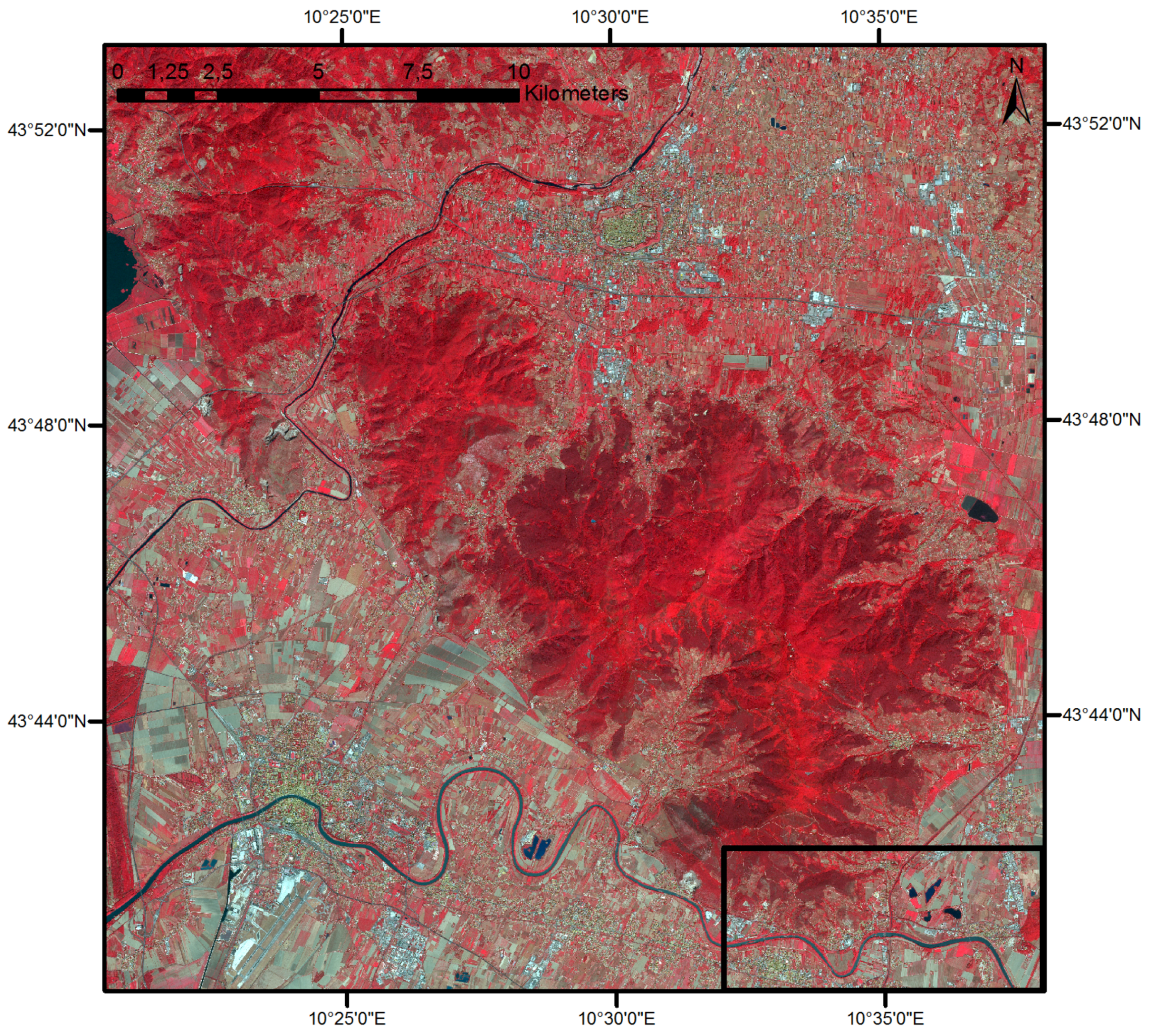
In this section, an example of the application of SML information extraction is provided. The purpose is purely demonstrative and didactic. Figure 2 shows the selected data sample in an RGB “false-color” composite image. The selected data sample was available through the Copernicus program [38].

Figure 2.
The Spot 5 input image employed in the example, in an RGB “false-color” composite representation (the marked zone from the bottom right corresponds to the area presented in Figure 3).
The data were collected in 2012 by the Spot 5 satellite that is equipped with a panchromatic and a multispectral sensor (supporting 2.5 and 10 m of spatial resolution, respectively), covering the towns of Pisa and Lucca in the Tuscany region of Italy. The images were available as pan-sharpened products with three multispectral channels (green, red and near infrared) sharpened at the resolution of the panchromatic one. No detailed metadata regarding the pre-processing procedure, including the exact parameters used for image data calibration and pan-sharpening, were available at the time of the test. De facto, this would have prevented the application of any physical-deterministic information retrieval tasks. In this showcase, the image data are ingested as-is in the feature extraction and classification processes. The rules linking image features to the target information are discovered by automatic inference in the SML procedure.
Morphological multiscale and radiometric image descriptors have been used as input for the SML showcase in the example. A brief description of their derivation follows. A luminance channel was calculated as the point-wise maximum of the red and green visible channels . The luminance was used as the input of a multi-scale morphological decomposition based on the characteristic saliency leveling (CSL) model [39]. The CSL model used lambda = [0, 80, 800, 8000] pixels corresponding to the scales of 0, 500, 5000, and 50,000 m2, with 2.52 = 6.25 m2 to be the surface of the pixel. Thus, the sequencing was made using six image descriptors: three of them derived from the CSL and the other three from the radiometric information stored in the green (G), red (R) and near infrared (NIR) image channels. The characteristic (C) layer of the CSL was not quantized, because it has inherently a symbolic representation, coded in seven symbols (3 + 3 scales in the concave and convex signal domains, plus the flat code 0). The saliency (S), leveling (L), G, R and NIR layers were quantized into eight levels.
The high-abstraction semantic layer Y used in the example as the reference set was derived from the Corine Land Cover (CLC) 2006 database (available at http://www.eea.europa.eu/data-and-maps/data/clc-2006-vector-data-version-3). The data were accessed at 100 m × 100 m of spatial resolution. As already mentioned in the Introduction, this is the typical scenario of the SML classifier. A redundant description of the same land surface is provided by different geo-spatial information sources. The link between the two sources is exclusively the spatial encoding. No harmonization of scale and thematic contents is postulated for the exercise. In this showcase, the image features extracted from the Spot 5 data to be classified and the classification of other satellite data embedded in the CLC final product are available and are describing the same land surface. CLC is considered a proxy of the information contained in the Spot 5 satellite image that must be detected. This proxy describes the whole universe of data with a given abstract thematic content (in both spatial and temporal domains). In this example, the spatial scale difference between the two sources is equal to 1002/2.52 = 1600 image samples for each reference sample, and the temporal difference is six years. In the showcase, the expert selects in the reference data the positive and negative examples to provide to the SML according to the specific classification needs. After that, the reference data are downscaled via nearest neighbor interpolation to reach the spatial resolution of the input features. Then, the machine automatically analyzes the relationships between the data instances (sequences) and the reference instances through association analysis and calculates the ENDI measure that may be used for the classification purposes.
For the purpose of this example, the original encoding (Corine Land Cover Legend http://sia.eionet.europa.eu/CLC2006/CLCLegeng.pdf) was re-coded into eight classes according to the classes grid codes (z) as follows: , , , , , , , , .
3.1. On Sequencing
Figure 4 shows the quantization sequencing obtained in the data example: for each row (in total, 2268 rows in the figure), the values of the input features and of for the selected land cover classes are represented column-wise. In this case, the ENDI measure is used; analogous observations can be derived from the and indices. From left to right, the first six columns represent the input image features: (1) the morphological characteristic C; (2) the saliency S; and (3) the leveling L; and the spectral bands: (4) green G; (5) red R; and (6) near infrared NIR. The data sequences are the rows consisting of the values of these first six columns. The next columns show the values of ENDI for each sequence, measuring the association between the image data instances and eight different CLC classes: water (7); agricultural (8); generic forest (9); broad-leaved forest cover (10); coniferous forest cover (11); generic urban (12); industrial areas (13); and residential areas (14). The used color code rises from black (lowest level) to dark-red (highest level). The color map was applied per column; that means, there is not a straightforward connection between the colors of adjacent columns. The coding of the first six columns denotes the quantized values of the input features, while for the remaining columns, it represents the ENDI values.
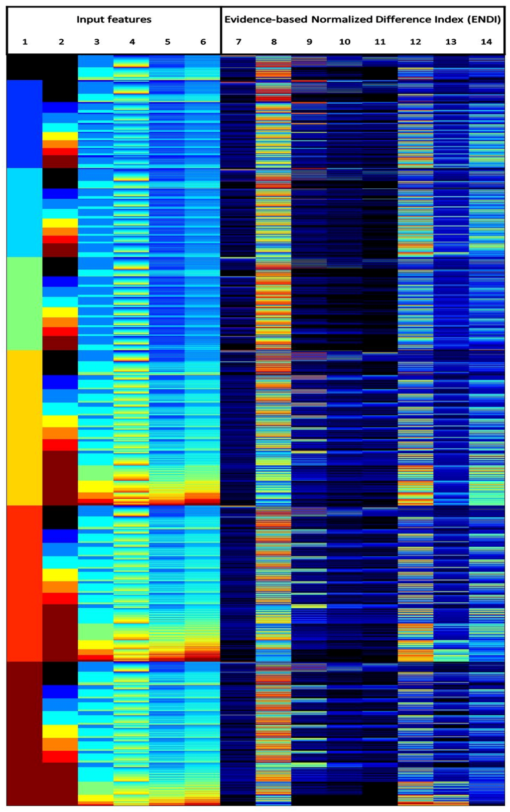
Figure 4.
Sequences obtained using the Spot 5 data and the Corine Land Cover (CLC) reference. From left to right, the first six columns represent the quantized values of the input image features: (1) C, (2) S, (3) L, (4) G, (5) R and (6) NIR. The following columns show the ΦE values for eight CLC classes: water (7), agricultural (8), generic forest (9), broad-leaved forest cover (10), coniferous forest cover (11), generic urban (12), industrial areas (13) and residential areas (14).
In general, very sharp boundaries of the can be observed in Figure 4. This means that, in some cases, very small variations in the image feature values may generate quite large effects on the decision about class membership based on learned confidences. Such a sharp and detailed behavior of the decision map is very difficult to obtain using continuous discriminant functions in the image feature space. It is worth noting that most of the standard classifiers (both parametric and non-parametric) used in remote sensing postulate the continuity of the discriminant functions: consequently, they are expected to produce much more simplified or blurred decision boundaries. Some classes (such as water (7), forest (9), broad-leaved (10) and coniferous (11)) show a more compact distribution in the feature space, as compared to agricultural (8) and urban (12), for example, which seem much more spread in the sequence list and, consequently, in the feature space. This compact distribution can be explained by the fact that they are pure classes describing almost the same physical characteristics in the same abstraction, then translated into a specific set of sequences delimiting a compact region in the feature space. On the other hand, classes, such as agricultural and urban, typically aggregate in the same abstraction very different physical characteristics, especially if observed in only one arbitrary point in time, as in the proposed example. Thus, they are translated into a discriminant function assuming complex and spread patterns in the whole feature space. While the pure classes are relatively easy to describe with continuous functions, the latter would be much more difficult. Finally, a kind of complementarity can be observed between the classes: if, in a specific data sequence and in a specific class, high values are observed, then the other classes generally show lower values. The other way around also applies. This characteristic allows one to apply the HDI techniques for the estimation of inter-class separability.
3.2. On Class Separability
The can be used to estimate the class separability given a set of data sequences. The more the classes are complementary regarding their distribution, the more they are separable based on the specific set of data sequences in use. This principle can be generalized and quantified using the HDI translated into the data sequences and domains. The HDI between two classes characterized by their probability density functions is defined as the complement of the ratio between the integral of the intersection and the integral of the union of the two histogram frequency density functions [21]. The HDI is a number in the range of [0, 1], having the zero value in the case of complete overlapping of the different probability density functions and the value of “1” in the case of complete separation. Table 1 presents the inter-class separation capability of the discriminant function as defined by in the feature space using the sequencing as shown in Figure 4.

Table 1.
Class separability by the histogram distance index (HDI) of the ΦE on data sequences generated from Spot 5 satellite data. Top: mutual class separability based on joint sequencing of morphological multiscale (characteristic saliency leveling (CSL)) and radiometric image descriptors. Bottom: average class separability for different sequencing options. CSLRAD joint morphological and radiometric descriptors; CSL morphological descriptors only; RAD radiometric descriptors only.
The table is produced by calculating the HDI values for each pair of CLC classes adopted in the example. Some class-specific considerations can be extracted from the table. For example, it can be noticed that the water class is well separated from all of the other classes showing generally high HDI values, while the agricultural class shows a relatively low separability score with the urban class (0.6902): this may be empirical evidence of the scattered rural settlement pattern existing in the area used as an example, and it should be further analyzed for improvement of the specific classification scheme. Similar considerations can be extracted regarding the other classes and are not included here.
These HDI measures can be helpful for the general evaluation of the goodness of the SML information extraction model, the suitability of the quantization scheme applied and the suitability of the image features used as input for discrimination of the target classes. Moreover, they can be used in the feature selection phase for the evaluation of the overall discrimination performances of different sets of input features. For example, at the bottom of Table 1, the total average HDI inter-class scores for three alternative sequencing approaches are reported. CSLRAD, CSL and RAD options select the integrated morphological and radiometric, morphological only and radiometric only features, respectively. It can be observed that the integrated CSLRAD option appears the best, separating the target classes with a total HDI of 0.8716 as compared to the CSL and RAD options that get a total HDI of 0.8546 and 0.8542, correspondingly, if used separately. Going deeper into the analysis, it could be interesting to notice that in the data used as an example, the CSL-only sequencing option seems to best separate the classes related to the urban fabric, while the RAD-only sequencing option works better in separating coniferous and broad-leaves forest classes. This can be supported by empirical evidence on known characteristics of the target classes. Urban fabric is made of heterogeneous materials with various mixing spatial patterns, but it is also made of the structures included in a specific range of scales (sizes), as compared to the other structures present in the image. Thus, at the input resolution of the sensor considered in the example, the CSL features better separate them compared to the RAD ones. On the other hand, broad-leaves and coniferous classes, if observed in only one point in time, are mostly distinguishable from the background because of their specific radiometric characteristics, and this is translated into the HDI values of the RAD-only sequencing option. Remarkable is also the fact that the industrial class is best separated by the integrated CSLRAD sequencing option (0.8840) scoring better than the CSL-only option (0.8723). This confirms the observation that the specific class is made by structures having unique morphological characteristics and the explicit reflectance signature generated by more uniform building practices, compared to the residential and urban classes in general.
3.3. On Classification
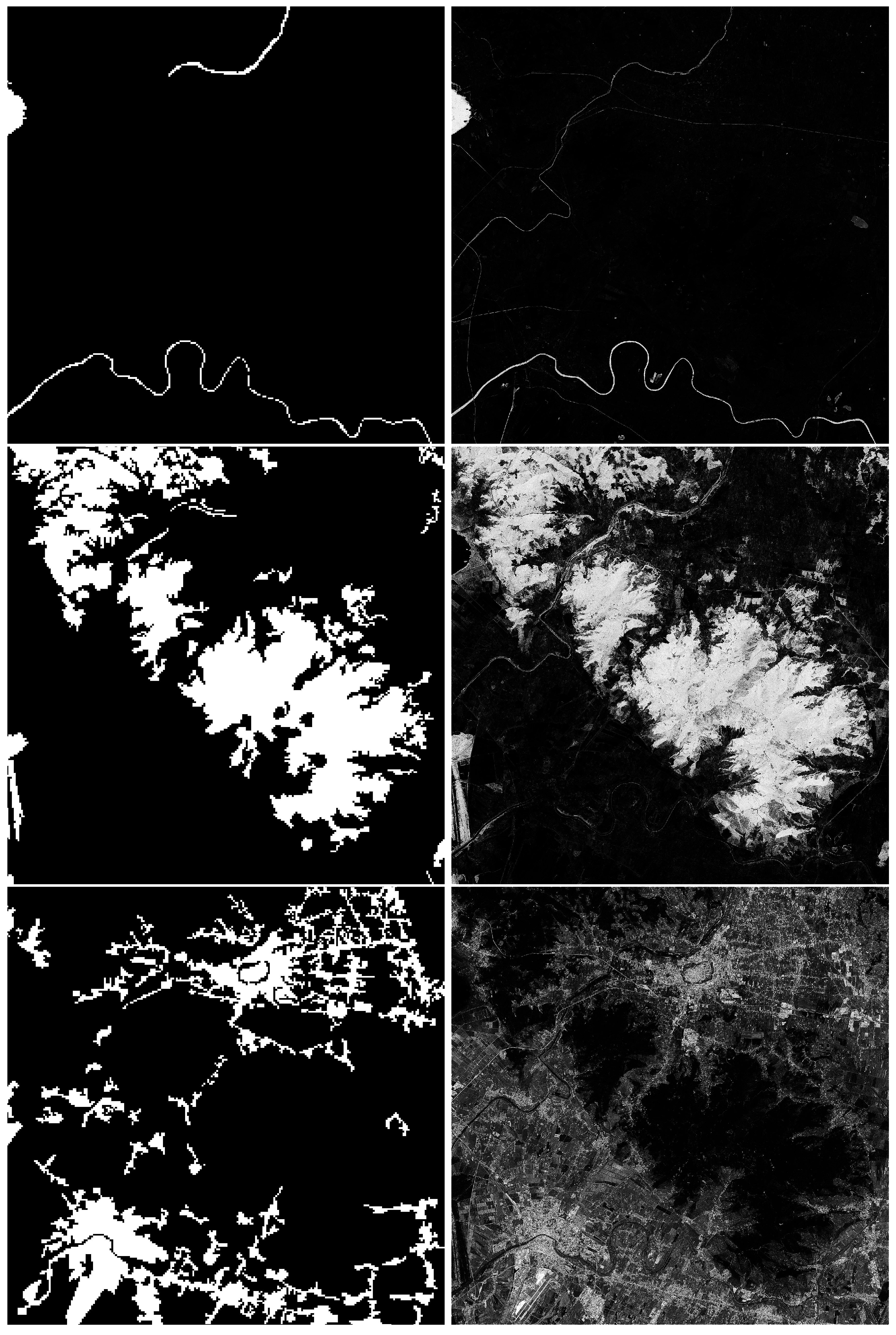
Figure 5 shows some examples of the mapped to the spatial domain of the image, for some of the CLC classes discussed here. The left column contains the high-abstraction semantic layers C (C ≡ Y), while on the right column, there are the corresponding of the image data sequences. In the images, the color code is from black () to white (). In these images, the zero level of the corresponds to 50% gray. From top to bottom; the reference set and the related to the classes of water, generic forest and generic urban are displayed. From these examples, we can see that the SML classifier output may significantly contradict the information provided by the reference set if the evidence collected from the image data sufficiently supports this decision; for instance, thin water channels and small water bodies have been identified and classified accordingly. Similarly, for the generic urban CLC class, several scattered settlements, thin structures or open spaces are identified even if neglected by the reference.

Figure 5.
The reference images (left) and the respective images of ΦE values (right) for water (top), generic forest (center) and generic urban (bottom) classes.
As already introduced, the output maps report the association between image data instances and high-level abstraction semantics or supervisory signals. They can be used as input for subsequent steps of classification in several ways. If a binary classification is required by the specific application, it can be derived by thresholding the outputs. Both single and multiple-class approaches can be designed as in [19,20]. A large variety of unsupervised or supervised techniques can be applied when searching for the optimal thresholding in the single or multiple , but they are not discussed in this manuscript. In [16], some supervised techniques are introduced and evaluated for classification accuracy and robustness against noise.
The outputs can also be interpreted as memberships to the target classes when using fuzzy or continuous logic multi-criteria frameworks. A simple application follows: let be the membership to the class c ∈ C = {other, water, generic forest, generic urban} obtained by a simple linear rescaling of the in the range [0, 1]. Let be the memberships to the classes water, generic forest and generic urban as estimated using the CLC land cover reference data and the satellite input data instances sequenced in their morphological and radiometric features. Let the membership be the complement of the union (calculated as the point-wise maximum) of the three considered class memberships expressing the background information or the anything else membership class. Then, the class of the data X can be estimated by maximization of the memberships as: .
Figure 6 displays the classification output by considering input data shown in Figure 2. The applied sequencing uses morphological and radiometric image features, as shown in Figure 4. The pixels that are classified to the four classes—other, water, generic forest and generic urban—are represented in black, blue, green and white colors, respectively. The classification was made through the ranking of their memberships to these four classes and derived from the estimated ENDI values.
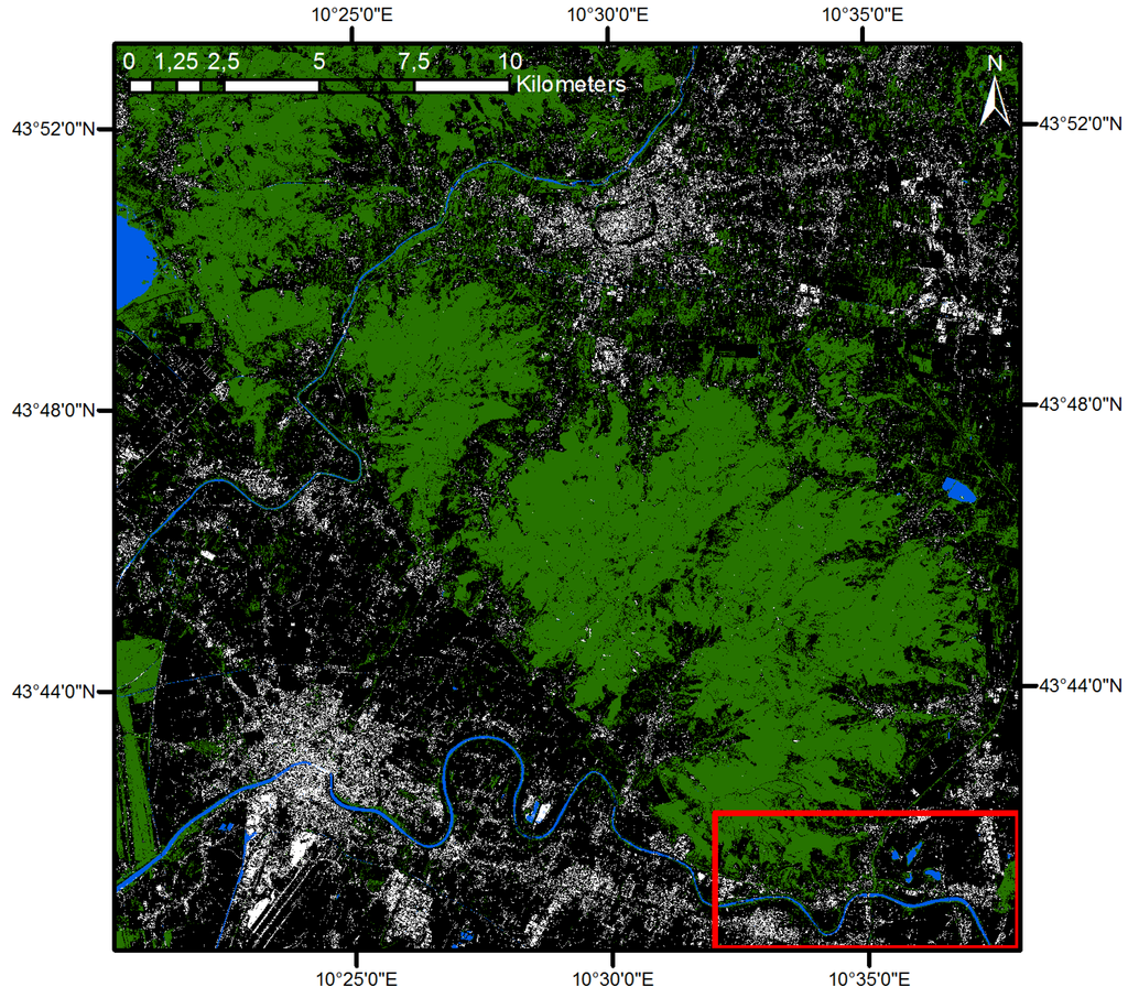
Figure 6.
The classification result when considering the following target classes: water (blue), generic forest (green), generic urban (white) and other (black).
Figure 3 illustrates the same classification exercise in a subset of the data corresponding to the region marked in Figure 2 and Figure 6: (top) the “false color” composite representation of the input data, (center) the classes used as the reference set for the SML, extracted from the CLC source having 100 m of spatial resolution, (bottom) the output of the classification procedure at 2.5 m of spatial resolution. The color coding is the same as in Figure 6. We can notice the increased detail of the classification output based on image data instances with a finer scale than the land cover data used as the supervisory signal by the SML. Furthermore, the presence of large fields with bare soil can be noticed in the input image. In standard classifiers, these targets are often confused with urban surfaces because of their similarity with the reflectance of roofing materials, road pavements and similar. The reasons why the proposed approach performs better in the discrimination of complex targets, like urban surface from bare soil, as shown in the specific example, are: (i) the capacity of SML to include seamlessly symbolic (morphological multiscale) and quantitative (radiometric multi-band reflectance) input features permitting the estimation of their joint contribution directly; and (ii) the distribution-free approach of SML that makes inferences in a pure data-driven way turns out in practice to partition the feature space effectively and decompose the intermixed signals accurately.
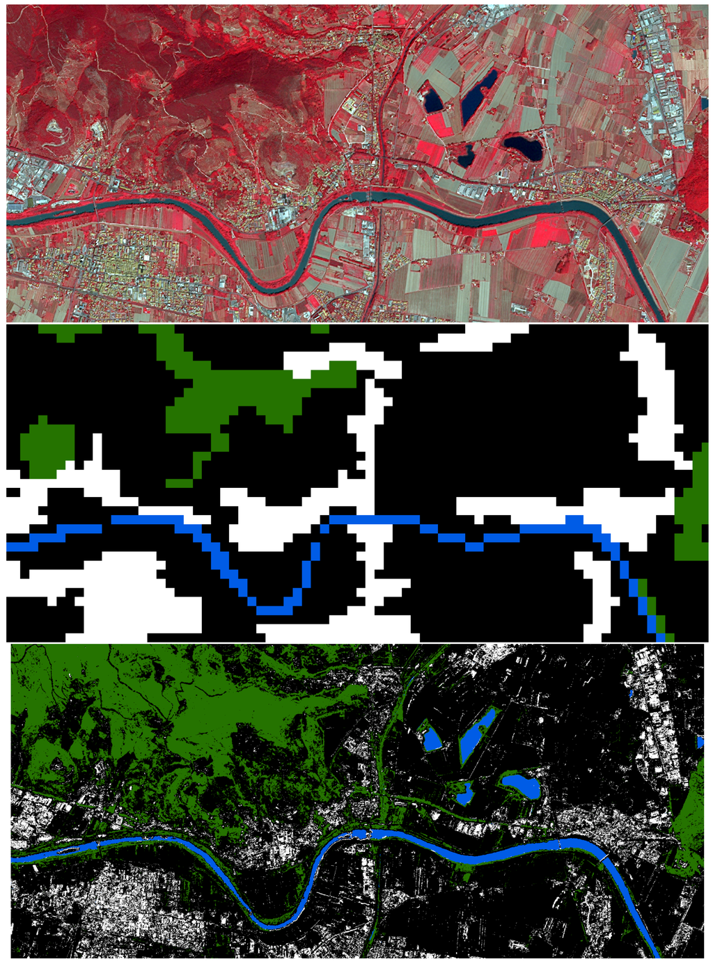
Figure 3.
The SML classification. Top: input data in “false color” composite; center: classes of the reference set extracted from the CLC source at a 100-m spatial resolution: water (blue), generic forest (green), generic urban (white) and other (black); bottom: result of SML classification at a 2.5-m spatial resolution.
4. Conclusions
A new method for supervised classification of remotely-sensed data was presented by analogy with the classification techniques used in bioinformatics and genome expression analysis. The method is defined in the frame of symbolic learning, and it is based on two main steps (i) data quantization-sequencing; and (ii) association analysis. In the application presented here, the quantization-sequencing process employs a uniform quantization, and it is independent from assumptions about specific statistical distributions. These choices allow the increase of computational efficiency and classification performance. The association analysis quantifies the associations between multi-attribute data sequences and available high-abstraction semantic layers used as a reference. The quantification takes place through ENDI (evidence-based normalized differential index), a new measure inspired by probability-based objective interestingness measures.
A land cover mapping application of SML techniques to 2.5-m resolution satellite data was presented, as well. The input image features were morphological multi-scale (CSL) and radiometric (G, R, NIR) descriptors. A subset of eight classes from the Corine Land Cover (CLC) available at 100 m of spatial resolution was used as the reference source for the training phase. Some considerations related to the data sequencing, the class separability and possible options for solving the final classification step were also presented.
The competitive characteristics of the proposed method for satellite data analytics are briefly listed below:
- The input data values are treated as symbols and not as numbers, a feature that facilitates the data fusion with nominal and categorical variables.
- It is a non-parametric technique. The learning is driven by the data and in particular by the pattern appearance frequency in each class. This feature facilitates the data fusion of heterogeneous sources having different statistical distributions that are not known or it is very difficult to approximate.
- The workflow is controlled by very few, easily tunable parameters and can be modulated effortlessly and smoothly to any low to moderate computing machinery.
- The algorithm’s computational complexity turns out to be adequate in the context of big data analytics.
- Given a specific quantization parameter set and the same input data, the SML classification provides a fully automatic and repeatable result.
- The method provides inferential rules easily understandable by humans.
The strength of the SML classifier consists in the fact that it is largely agnostic both with respect to the statistical distribution of the input data and to the relationships between the image data and the information to be detected. It can constitute an efficient candidate for large-scale processing that runs smoothly within the big data context [17]. Furthermore, it has proven to be robust and able to extract complex information in the presence of noisy reference sets [16].
Finally, it is worth noting that the last two items of the list above (full repeatability and easy interpretation of the detected rules) facilitate the use of satellite-derived information products in evidence-based decision support processes.
On the other hand, weak points related to the new method as proposed in this manuscript are related to the combinatorial nature of the approach. The risk of over-fitting the data increases by augmenting the number of features or by increasing the length of the data sequences. A trade-off between the number of features and the number of encoded symbols must be taken into account in order to avoid such risk. Another weak point is its dependence on the quality of the data. Even if experiments exhibit a good level of robustness against noisy data, the fact that the inferences are drawn through a pure data-driven mechanism makes the validation of the results complex. Mitigation measures can be taken to reduce this risk by including tests on class separability based on observation of ΦE distributions and by including knowledge-driven reasoning in the general classification design, as proposed, for example, in [19].
The next interesting research topics related to SML classifier will be the testing of inter-scene model transferability and generalization, the development of adaptive feature selection and quantization sequencing techniques, the testing of alternative measures in the association analysis phase and the experimentation with supervised and unsupervised thresholding techniques and other classification indices.
Acknowledgments
The work was supported by the European Commission’s Joint Research Centre institutional work program relative to the Global Human Settlement Layer (GHSL) project. The authors would like to thank the whole GHSL team for the substantial help provided during all of the phases of the experimental activities reported in this manuscript.
Author Contributions
Martino Pesaresi designed and made the first prototype of the SML method. Andreea Julea assessed the method in the association analysis and interestingness measures frameworks. Vasileios Syrris engineered the SML prototype and assessed the method from the perspective of the computational complexity and memory load. All of the authors equally contributed to the drafting of the results included in the manuscript and to the related data processing activities.
Conflicts of Interest
The authors declare no conflict of interest.
References
- Campbell, J.B.; Wynne, R.H. Introduction to Remote Sensing; Guilford Press: New York, NY, USA, 2011. [Google Scholar]
- Avery, T.E.; Berlin, G.L. Fundamentals of Remote Sensing and Airphoto Interpretation; Macmillan: New York, NY, USA, 1992. [Google Scholar]
- Verstraete, M.M.; Pinty, B.; Myneni, R.B. Potential and limitations of information extraction on the terrestrial biosphere from satellite remote sensing. Remote Sens. Environ. 1996, 58, 201–214. [Google Scholar] [CrossRef]
- Craglia, M.; de Bie, K.; Jackson, D.; Pesaresi, M.; Remetey-Fülöpp, G.; Wang, C.; Annoni, A.; Bian, L.; Campbell, F.; Ehlers, M.; et al. Digital Earth 2020: Towards the vision for the next decade. Int. J. Digit. Earth 2012, 5, 4–21. [Google Scholar] [CrossRef]
- Yang, J.; Gong, P.; Fu, R.; Zhang, M.; Chen, J.; Liang, S.; Xu, B.; Shi, J.; Dickinson, R. The role of satellite remote sensing in climate change studies. Nat. Clim. Chang. 2013, 3, 875–883. [Google Scholar] [CrossRef]
- Goodchild, M.F. Citizens as sensors: The world of volunteered geography. GeoJournal 2007, 69, 211–221. [Google Scholar] [CrossRef]
- Woodcock, C.E.; Allen, R.; Anderson, M.; Belward, A.; Bindschadler, R.; Cohen, W.; Gao, F.; Goward, S.N.; Helder, D.; Helmer, E.; et al. Free access to Landsat imagery. Science 2008, 320. [Google Scholar] [CrossRef] [PubMed]
- Soille, P.; Burger, A.; Rodriguez, D.; Syrris, V.; Vasilev, V. Towards a JRC Earth Observation Data and Processing Platform. In Proceedings of the Conference on Big Data from Space (BiDS’16), Santa Cruz de Tenerife, Spain, 15–17 March 2016.
- Pesaresi, M. Global Fine-Scale Information Layers: The Need of a Paradigm Shift. In Proceedings of the Conference on Big Data from Space (BiDS’14), Esrin, Italy, 12–14 November 2014; pp. 8–11.
- Van Zyl, T. Machine Learning on Geospatial Big Data. In Big Data: Techniques and Technologies in Geoinformatics; Karimi, H.A., Ed.; CRC Press: Boca Raton, FL, USA, 2014; pp. 133–148. [Google Scholar]
- Samuel, A.L. Some studies in machine learning using the game of checkers. IBM J. Res. Dev. 1959, 3, 210–229. [Google Scholar] [CrossRef]
- Becquet, C.; Blachon, S.; Jeudy, B.; Boulicaut, J.F.; Gandrillon, O. Strong-association-rule mining for large-scale gene-expression data analysis: A case study on human SAGE data. Genome Biol. 2002, 3, 1–16. [Google Scholar] [CrossRef]
- Creighton, C.; Hanash, S. Mining gene expression databases for association rules. Bioinformatics 2003, 19, 79–86. [Google Scholar] [CrossRef] [PubMed]
- Georgii, E.; Richter, L.; Rückert, U.; Kramer, S. Analyzing microarray data using quantitative association rules. Bioinformatics 2005, 21, ii123–ii129. [Google Scholar] [CrossRef] [PubMed]
- Anandhavalli, M.; Ghose, M.K.; Gauthaman, M. Association Rule Mining in Genomics. Int. J. Comput. Theory Eng. 2010, 2, 269–273. [Google Scholar] [CrossRef]
- Pesaresi, M.; Syrris, V.; Julea, A. Benchmarking of the Symbolic Machine Learning Classifier with State of the Art Image Classification Methods—Application to Remote Sensing Imagery; JRC Technical Report; European Commission, Joint Research Centre, Institute for the Protection and Security of the Citizen: Ispra, Italy, 2015. [Google Scholar]
- Pesaresi, M.; Syrris, V.; Julea, A. Analyzing big remote sensing data via symbolic machine learning. In Proceedings of the 2016 Conference on Big Data from Space (BiDS’16), Santa Cruz de Tenerife, Spain, 15–17 March 2016.
- Mayer-Schönberger, V.; Cukier, K. Big Data: A Revolution That Will Transform How We Live, Work, and Think; Houghton Mifflin Harcourt: New York, NY, USA, 2013. [Google Scholar]
- Pesaresi, M.; Ehrlich, D.; Ferri, S.; Florczyk, A.; Freire, S.; Halkia, M.; Julea, A.; Kemper, T.; Soille, P.; Syrris, V. Operating Procedure for the Production of the Global Human Settlement Layer from Landsat Data of the Epochs 1975, 1990, 2000, and 2014; JRC Technical Report; European Commission, Joint Research Centre, Institute for the Protection and Security of the Citizen: Ispra, Italy, 2015. [Google Scholar]
- Pesaresi, M.; Corbane, C.; Julea, A.; Florczyk, A.J.; Syrris, V.; Soille, P. Assessment of the Added-Value of Sentinel-2 for Detecting Built-up Areas. Remote Sens. 2016, 8, 299. [Google Scholar] [CrossRef]
- Pesaresi, M. Texture Analysis for Urban Pattern Recognition Using Fine-resolution Panchromatic Satellite Imagery. Geogr. Environ. Model. 2000, 4, 43–63. [Google Scholar] [CrossRef]
- Hedges, T. An empirical modification to linear wave theory. Proc. Inst. Civ. Eng. 1976, 61, 575–579. [Google Scholar]
- Cha, S.H. Comprehensive Survey on Distance Similarity Measures between Probability Density Functions. Int. J. Math. Models Methods Appl. Sci. 2007, 1, 300–307. [Google Scholar]
- Pesaresi, M.; Huadong, G.; Blaes, X.; Ehrlich, D.; Ferri, S.; Gueguen, L.; Halkia, M.; Kauffmann, M.; Kemper, T.; Lu, L.; et al. A Global Human Settlement Layer From Optical HR/VHR RS Data: Concept and First Results. IEEE J. Sel. Top. Appl. Earth Observ. Remote Sens. 2013, 6, 2102–2131. [Google Scholar] [CrossRef]
- Bailey, K.D. Typologies and Taxonomies: An Introduction to Classification Techniques. In Quantitative Applications in the Social Sciences; SAGE Publications, Inc.: Thousand Oaks, CA, USA, 1994; Volume 102. [Google Scholar]
- Everitt, B.S.; Landau, S.; Leese, M.; Stahl, D. An Introduction to Classification and Clustering. In Cluster Analysis, 5th ed.; John Wiley & Sons, Ltd.: Chichester, UK, 2011; pp. 1–13. [Google Scholar]
- Zepeda, J.; Guillemot, C.; Kijak, E. Image Compression Using Sparse Representations and the Iteration-Tuned and Aligned Dictionary. IEEE J. Sel. Top. Signal Process. 2011, 5, 1061–1073. [Google Scholar] [CrossRef]
- Wright, J.; Ma, Y.; Mairal, J.; Sapiro, G.; Huang, T.S.; Yan, S. Sparse representation for computer vision and pattern recognition. Proc. IEEE 2010, 98, 1031–1044. [Google Scholar] [CrossRef]
- Zhang, L.; Zuo, W.; Zhang, D. LSDT: Latent Sparse Domain Transfer Learning for Visual Adaptation. IEEE Trans. Image Process. 2016, 25, 1177–1191. [Google Scholar] [CrossRef] [PubMed]
- Mairal, J.; Ponce, J.; Sapiro, G.; Zisserman, A.; Bach, F.R. Supervised Dictionary Learning. In Advances in Neural Information Processing Systems 21: 22nd Annual Conference on Neural Information Processing Systems 2008; Curran Associates, Inc.: Red Hook, NY, USA, 2008; pp. 1033–1040. [Google Scholar]
- Liu, H.; Hussain, F.; Tan, C.; Dash, M. Discretization: An Enabling Technique. Data Min. Know. Discov. 2002, 6, 393–423. [Google Scholar] [CrossRef]
- Liu, B.; Hsu, W.; Ma, Y. Integrating Classification and Association Rule Mining. In Proceedings of the International Conference on Knowledge Discovery and Data Mining (KDD’98), New York, NY, USA, 27–31 August 1998; pp. 80–86.
- Tew, C.; Giraud-Carrier, C.; Tanner, K.; Burton, S. Behavior-based clustering and analysis of interestingness measures for association rule mining. Data Min. Know. Discov. 2014, 28, 1004–1045. [Google Scholar] [CrossRef]
- Geng, L.; Hamilton, H.J. Interestingness Measures for Data Mining: A Survey. ACM Comput. Surv. 2006, 38, 9. [Google Scholar] [CrossRef]
- Blanchard, J.; Guillet, F.; Briand, H.; Gras, R. Assessing rule interestingness with a probabilistic measure of deviation from equilibrium. In Proceedings of the 11th International Symposium on Applied Stochastic Models and Data Analysis, Brest, France, 17–20 May 2005; pp. 191–200.
- Ganascia, J. Charade: Apprentissage de bases de connaissances. In Induction Symbolique et Numérique à Partir de Données; Cépaduès Editions: Toulouse, France, 1991; pp. 309–326. [Google Scholar]
- Kodratoff, Y. Comparing Machine Learning and Knowledge Discovery in DataBases: An Application to Knowledge Discovery in Texts. In Machine Learning and Its Applications: Advanced Lectures; Paliouras, G., Karkaletsis, V., Spyropoulos, C., Eds.; Springer-Verlag: London, UK, 2001; pp. 1–21. [Google Scholar]
- Burger, A.; Di Matteo, G.; Åstrand, P.J. Specifications of View Services for GMES Core_003 VHR2 Coverage; JRC Technical Report; European European Commission, Joint Research Centre, Institute for Environment and Sustainability: Ispra, Italy, 2012. [Google Scholar]
- Pesaresi, M.; Ouzounis, G.K.; Gueguen, L. A new compact representation of morphological profiles: Report on first massive VHR image processing at the JRC. In Proceedings of the SPIE 8390, Algorithms and Technologies for Multispectral, Hyperspectral, and Ultraspectral Imagery XVIII, Baltimore, MD, USA, 8 May 2012.


© 2016 by the authors; licensee MDPI, Basel, Switzerland. This article is an open access article distributed under the terms and conditions of the Creative Commons Attribution (CC-BY) license (http://creativecommons.org/licenses/by/4.0/).