Abstract
Several frequency-based spectral similarity measures, derived from commonly-used ones, are developed for hyperspectral image classification based on the frequency domain. Since the frequency spectrum (magnitude spectrum) of the original signature for each pixel from hyperspectral data can clearly reflect the spectral features of different types of land covers, we replace the original spectral signature with its frequency spectrum for calculating the existing spectral similarity measure. The frequency spectrum is symmetrical around the direct current (DC) component; thus, we take one-half of the frequency spectrum from the DC component to the highest frequency component as the input signature. Furthermore, considering the fact that the low frequencies include most of the frequency energy, we can optimize the classification result by choosing the ratio of the frequency spectrum (from the DC component to the highest frequency component) involved in the calculation. In our paper, the frequency-based measures based on the spectral gradient angle (SAM), spectral information divergence (SID), spectral correlation mapper (SCM), Euclidean distance (ED), normalized Euclidean distance (NED) and SID × sin(SAM) (SsS) measures are called the F-SAM, F-SID, F-SCM, F-ED, F-NED and F-SsS, respectively. In the experiment, three commonly-used hyperspectral remote sensing images are employed as test data. The frequency-based measures proposed here are compared to the corresponding existing ones in terms of classification accuracy. The classification results by parameter optimization are also analyzed. The results show that, although not all frequency-based spectral similarity measures are better than the original ones, some frequency-based measures, such as the F-SsS and F-SID, exhibit a relatively better performance and have more robust applications than the other spectral similarity measures.
1. Introduction
Hyperspectral data can provide hundreds of contiguous bands for spectral analysis simultaneously, and in a hyperspectral image, more details are available to describe the spectral information of ground objects than in a multi-spectral image. The hyperspectral data can be regarded as a spectral cube where the third dimensionality is the spectral domain due to the capability of continuous spectral capture. However, a problem arises in hyperspectral image classification (e.g., the Hughes phenomenon [1]). As the high dimensionality of hyperspectral data increases, the number of training samples for the classifier also increases.
In order to mitigate the influence of the Hughes phenomenon, dimensionality reduction is usually adopted before image classification. Feature extraction is important to dimensionality reduction for hyperspectral image analysis. Principal component analysis (PCA) [1,2] is still the commonly-used feature extraction algorithms. The main reason is that PCA can solve a linear and convex problem and is invertible. Independent component analysis (ICA) is also applied in the hyperspectral image analysis and presentation. Tu indicated that the noise-adjusted version of fast ICA offers a new approach for unsupervised signature extraction and separation in hyperspectral images [3]; Wang and Chang [4] developed an ICA-DRfor endmember extraction and data compression. Furthermore, Villa et al. [5] applied the ICA technique to hyperspectral classification. Farrell and Mersereau [6] and Li et al. [7] proposed local Fisher’s linear discriminant analysis (LDA) for dimensionality reduction in hyperspectral data before employing the Gaussian mixture model and support vector machine (SVM) classifier.
Furthermore, there are some more impressive algorithms. Zhang et al. used the tensor discriminative locality alignment [8] to remove the redundant information for hyperspectral image classification. Minimum noise fraction (MNF), which is a linear transform, projects data into a new space in order to split these data into two parts, one of which is associated with the original signal and another of which is considered as the noise. Thus, this method is used for band selection of the hyperspectral image [9,10]. Meanwhile, projection pursuit [11,12], clonal selection theory [13], and the random forest model [14,15] are applied to feature extraction for hyperspectral image.
Band selection is also an important tool for hyperspectral image analysis, except for the feature extraction technique. Guo et al. [16], and Sotoca and Pla [17] used mutual information to select bands from the hyperspectral image. Marin et al. [18] used genetic algorithm (GA) to select the band from a hyperspectral image. The experimental result by comparing it to the end-member and spectral unmixing approach shows that the GA is a promising method. Additionally, there is band add-on (BAO) [19] for band selection for hyperspectral image analysis.
After dimensionality reduction, traditional multi-spectral remote sensing image classification methods, such as maximum likelihood (ML) [20,21] and the Bayes classification method [22], are used to complete the subsequent classification.
Other advanced and popular approaches are kernel-based algorithms, such as SVMs [23], kernel Fisher discriminants (KFDs) [24,25], support vector clustering [26] and the regularized AdaBoost algorithm [27,28]. The advantage is that kernel-based approaches can be used to analyze hyperspectral data directly, without dimensionality reduction and band selection. SVMs, in particular, have been widely applied in the hyperspectral remote sensing image classification community [29,30,31]. The training time, although much smaller than that of other kernel-based algorithms, quadratically depends on the size of the training sample. Thus, it increases significantly, when a large number of labeled samples is available. Furthermore, there are other learning machine techniques, such as extreme learning machine [32,33].
Furthermore, extensive studies on spectral-spatial classification, which incorporate the spatial contextual information into pixel-wise classifiers, have been performed in the hyperspectral remote sensing community. These methods include segmentation based [34,35], morphological profile filtered [36], Markov random field [37,38] graph-cut [39,40] and many other ones. Additionally, researchers have also proposed other advanced methods, such as dictionary learning [41,42] and the Gaussian process [43], for hyperspectral data classification.
Meanwhile, metric-based algorithms that measure spectral similarity and discrimination between a target and reference spectral signature are popular in hyperspectral remote sensing image classification. The spectral similarity measurement is valuable and important for hyperspectral image analysis. In addition, it is extensively applied to ground-object identification and classification of hyperspectral remote sensing images. Richards and Jia [44] used the Euclidean distance (ED) to calculate as the spectral similarity using the Euclidean distance between two spectral vectors. Because ED only takes into account the brightness difference between two vectors, the ED is not sensitive to the shape and scaling of the spectral signature. Subsequently, the normalized Euclidean distance (NED) [45] is proposed to calculate the Euclidean distance between two spectra divided by the mean of the spectral signatures. Meanwhile, there are more efficient spectral similarity measures, such as spectral gradient angle (SAM) [46,47], spectral information divergence (SID) [48] and spectral correlation mapper (SCM) [49]. Especially, SAM, which is used to measure spectral similarity by retrieving the angle between two spectral signatures portrayed as vectors, is a commonly-used measure in this application. Furthermore, Du et al. [50] proposed two mixture spectral similarity measures based on the SID and SAM measures, namely SID × sin(SAM) (SsS) and SID × tan(SAM) (StS), which considerably increase spectral discriminability.
Fourier transform is an important tool in signal processing. In the research on hyperspectral image analysis, Salgado and Ponomaryov [51] proposed feature selection based on coefficients obtained via discrete Fourier transform (DFT). Furthermore, two-dimensional (2D) Fourier transform is applied for sharpening HSIdata [52].
The differences among the spectral signatures of different ground objects result in the discrepancy in the distribution of the frequency component’s magnitudes, namely the frequency spectrum, of these spectra. Thus, it indicates that we can use the frequency spectrum to analyze the availability of the existing spectral similarity measures. Based on this conclusion, Wang et al. [53,54] proposed two spectral similarity measures based on the frequency domain. Wang et al. [53] previously used the first few low-frequency components to produce the measure. To balance the difference between the low- and high-frequency components, the Canberra distance is introduced to increase the contribution from the higher frequencies. In the following research [54], the frequency spectrum of the target spectral signature is taken as the normalized factor to balance the lower and higher frequency components. In this paper, we use the frequency spectrum of the spectral signatures to calculate the spectral similarity measures based on the existing measures, including the SAM, SID, SCM, ED, NED, StS and SsS measures. First, the spectral signatures are Fourier transformed to obtain the frequency spectrum. Second, the transformed frequency spectrum is used for calculating the existing spectral similarity measure. Because the frequency spectrum is symmetric with respect to the direct current (DC) component, half of the frequency spectrum is involved in the calculation. Finally, the existing spectral similarity measures computed by using the frequency spectrum are compared to these original ones, in order to analyze the effectiveness of the frequency spectrum applied to obtain the spectral similarity measure for hyperspectral image classification and object recognition.
2. Methodology
2.1. Fourier Analysis of the Spectral Signature
Fourier analysis is one of the most frequently-used tools for signal processing, and its application is involved in many other scientific fields, such as physical science, engineering and pattern recognition. It is pointed out that a real-valued periodic period-p function can be expressed as the sum of sinusoidal oscillations of various frequencies, magnitudes and phase shifts [55]. Additionally, the process of calculating the Fourier coefficient is defined as the Fourier transform. A signal can be given by a complete description with sines and cosines. Let be a discrete signal; the Fourier transform of can be given by:
where u is the frequency. After the Fourier transform, a result of complex frequency is retrieved. The expression of polar coordinates can be defined by:
where and are the frequency spectrum (magnitude spectrum) and phase spectrum, respectively, and are given by:
Furthermore, the power spectrum can be given by:
In this paper, we use the frequency spectrum to analyze the spectral signature of each pixel in hyperspectral data. Because the signature is discrete, the frequency spectrum can be obtained by using the discrete Fourier transform (DFT) defined by:
where N is the length of the spectral signature. The inverse discrete Fourier transform (IDFT) is defined as:
2.2. Fourier Analysis of the Simulated Discrete Signal
Before the measurement of spectral similarity can be obtained using the frequency spectrum, the distribution of the simulated discrete signal is analyzed. Here, we focus on the analysis of the frequency and power spectrum for the representation of the optical spectral signature from the hyperspectral data. The frequency and power spectrum, which is the square function of the frequency spectrum, are different in physical significance, even though they seem similar. The frequency spectrum presents another distribution of the change intensity of the original signal strength, and it is arranged from low to high frequency components, in which the DC component has zero frequency. The power spectrum, which is arranged like the frequency spectrum, mainly describes the distribution of the original signal energy. The relation between the power spectrum and the original signal is expressed by:
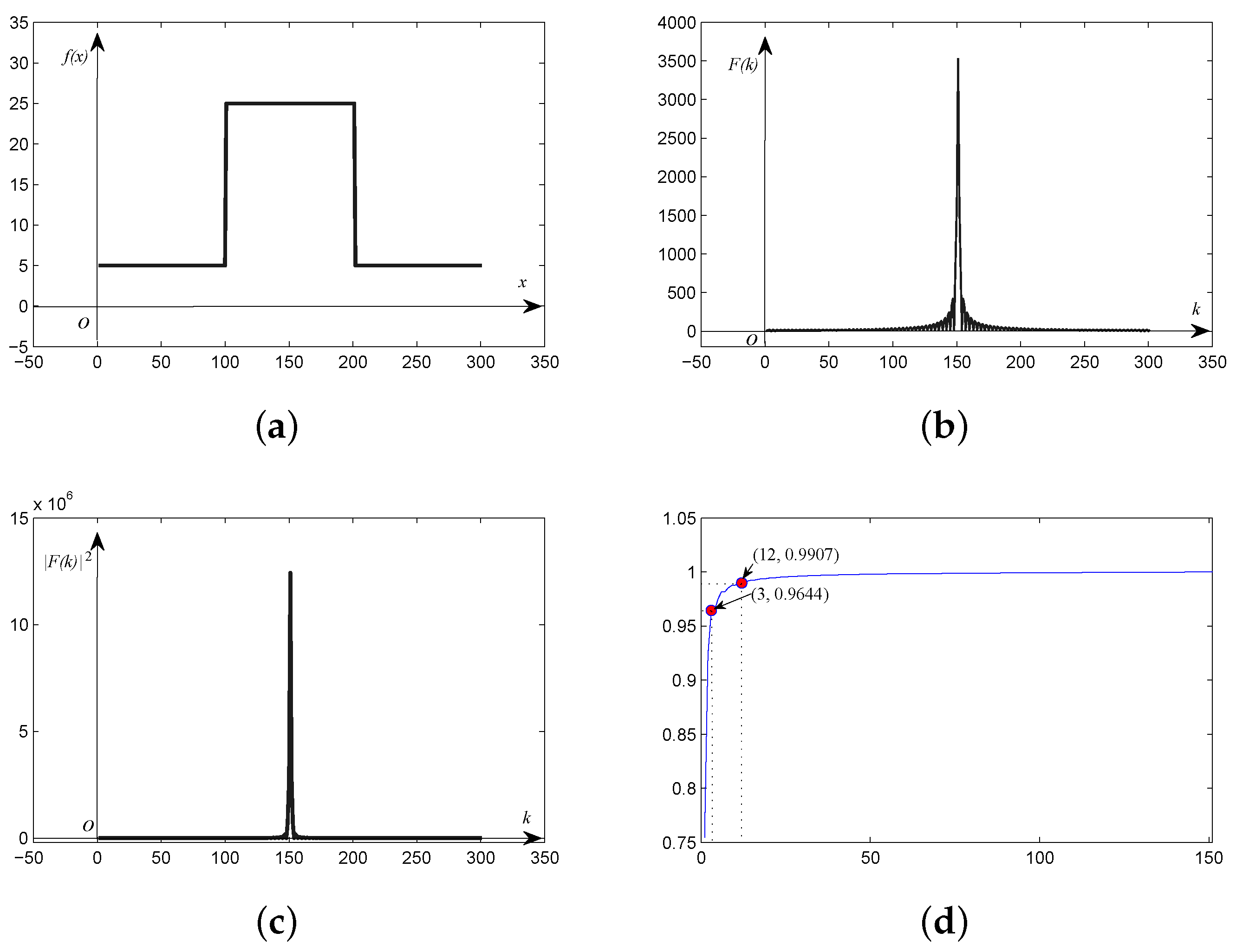
The one-dimensional simulated square wave discrete signal plotted in Figure 1a is taken as an example for frequency and power spectrum analysis. The frequency and power spectrum of the original signal are illustrated in Figure 1b,c, respectively. As shown in Figure 1b, we can see that the magnitude of the DC component is much higher than the other frequency components. Meanwhile, the magnitude of these frequency components decreases sharply with distance from the DC component. The tendency of the power spectrum is more distinct than that of the frequency spectrum, indicating that the energy of the spectral signature concentrates around the DC component. The curve shown in Figure 1d is the ratio of the frequency energy of the harmonics between the DC component and every other frequency component, to all frequency energy. It can be seen that the energy of the first three harmonics is up to 95%, and the energy of the first twelve harmonics is over 99%.

Figure 1.
(a) Square wave discrete signal; (b) frequency; and (c) power spectrum of the square wave signal; (d) ratio of frequency energy from the power spectrum.
To analyze the frequency spectrum of the real spectral signature, five typical spectral signatures, including water, anorthite, roscoelite, jarosite and lawn grass in the United States Geological Survey (USGS) reflectance spectral library, are taken as samples for experimental frequency spectrum analysis. Figure 2 shows that the five spectral signatures are markedly different from each other.
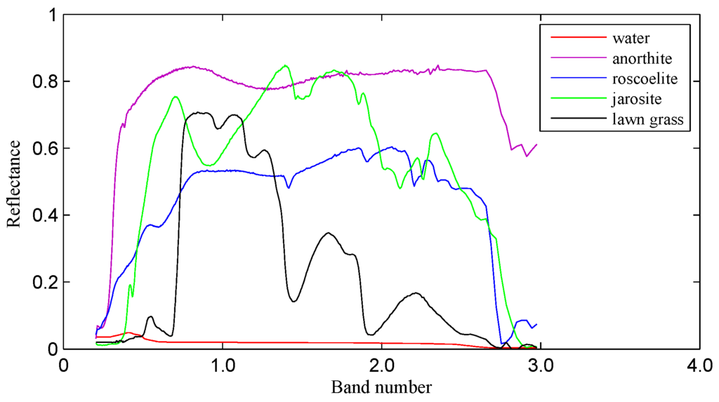
Figure 2.
Spectral signatures of water, anorthite, roscoelite, jarosite and lawn grass in the USGS spectral library.
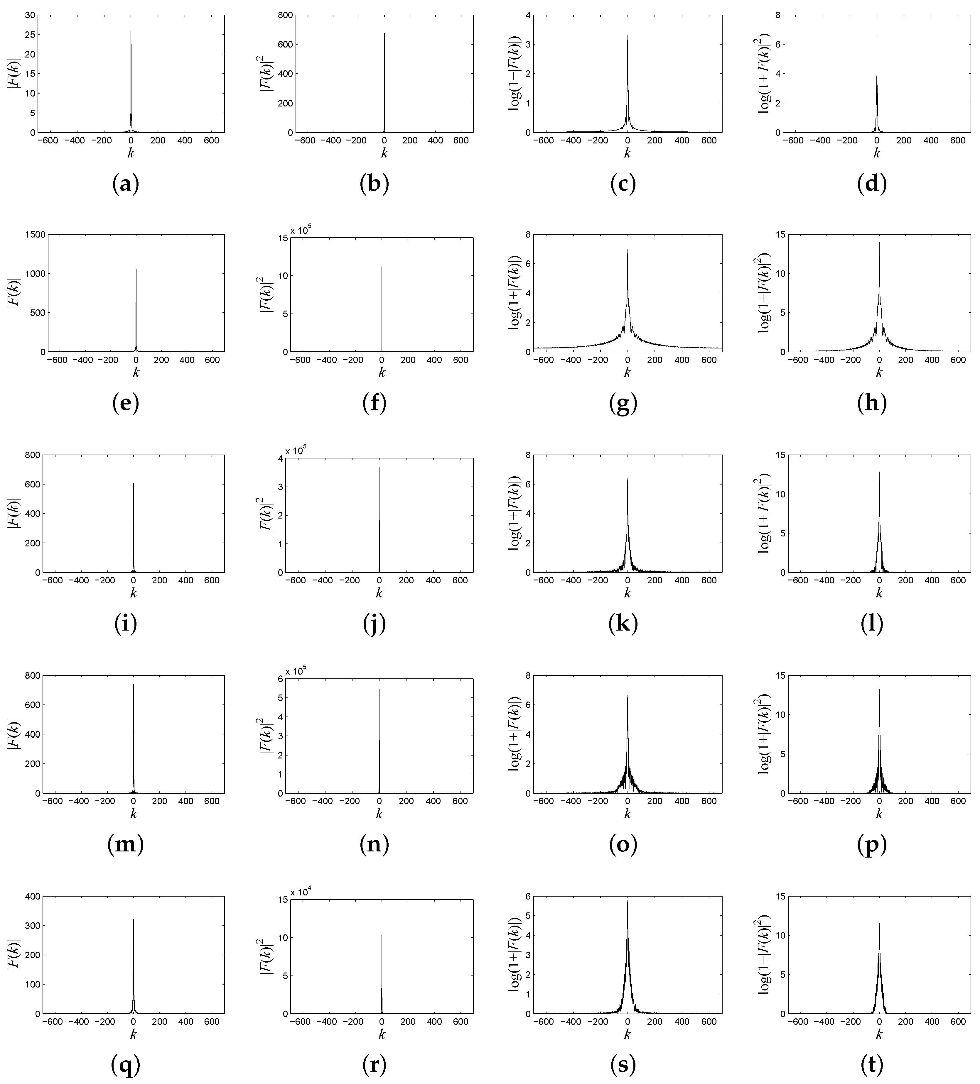
These five original spectral signatures are resampled to objectively analyze the distribution of the frequency spectrum and the power spectrum. As shown in Figure 2, the resampled interval is 0.02 m, and the final length of the resampled signature is 1385. Frequency spectrums of these spectral signatures are shown in the first column of Figure 3; power spectrums are shown in the second column of Figure 3. In order to clearly illustrate the difference between the frequency spectrum energy distribution from different ground objects’ spectral signatures, we plot the logarithmic form of the frequency spectrum and the power spectrum, which are shown in the third and fourth column of Figure 3, according to Equations (9) and (10). Note that most of the frequency energy is concentrated around the DC component, and the frequency spectrum energy of the high frequencies is much less.
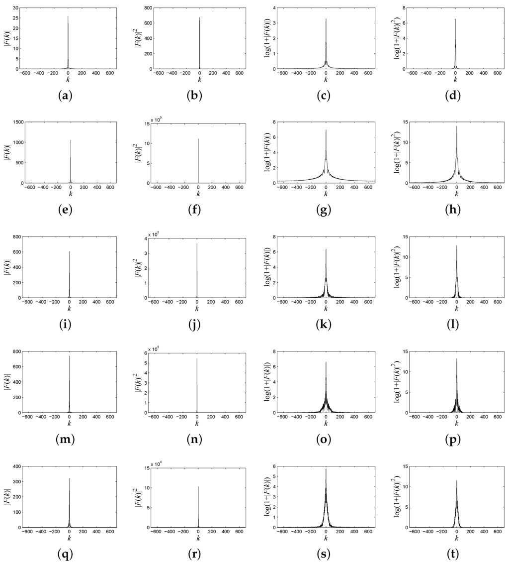
Figure 3.
(a) The frequency spectrum of the spectral signature of water; (b) the power spectrum of the spectral signature of water; (c) the logarithmic form of the frequency spectrum of the spectral signature of water; (d) the logarithmic form of the power spectrum of the spectral signature of water; (e) the frequency spectrum of the spectral signature of anorthite; (f) the power spectrum of the spectral signature of anorthite; (g) the logarithmic form of the frequency spectrum of the spectral signature of anorthite; (h) the logarithmic form of the power spectrum of the spectral signature of anorthite; (i) the frequency spectrum of the spectral signature of roscoelite; (j) the power spectrum of the spectral signature of roscoelite; (k) the logarithmic form of the frequency spectrum of the spectral signature of roscoelite; (l) the logarithmic form of the power spectrum of the spectral signature of roscoelite; (m) the frequency spectrum of the spectral signature of jarosite; (n) the power spectrum of the spectral signature of jarosite; (o) the logarithmic form of the frequency spectrum of the spectral signature of jarosite; (p) the logarithmic form of the power spectrum of the spectral signature of jarosite; (q) the frequency spectrum of the spectral signature of lawn grass; (r) the power spectrum of the spectral signature of lawn grass; (s) the logarithmic form of the frequency spectrum of the spectral signature of lawn grass; (t) the logarithmic form of the power spectrum of the spectral signature of lawn grass.
Evidently, as shown in Figure 3, there are remarkable differences of the frequency and power spectrum characteristics among the five typical spectral signatures. For example, the DC component of water’s spectral signature in Figure 3a–d is much lower than that of the other ground objects. Since most of frequency energy concentrates about the DC component, the declines of these five signatures are similar to each other. However, the rate of decline in the frequency spectrum from the DC component to high frequency components is different among these five typical ground objects’ spectral signatures.
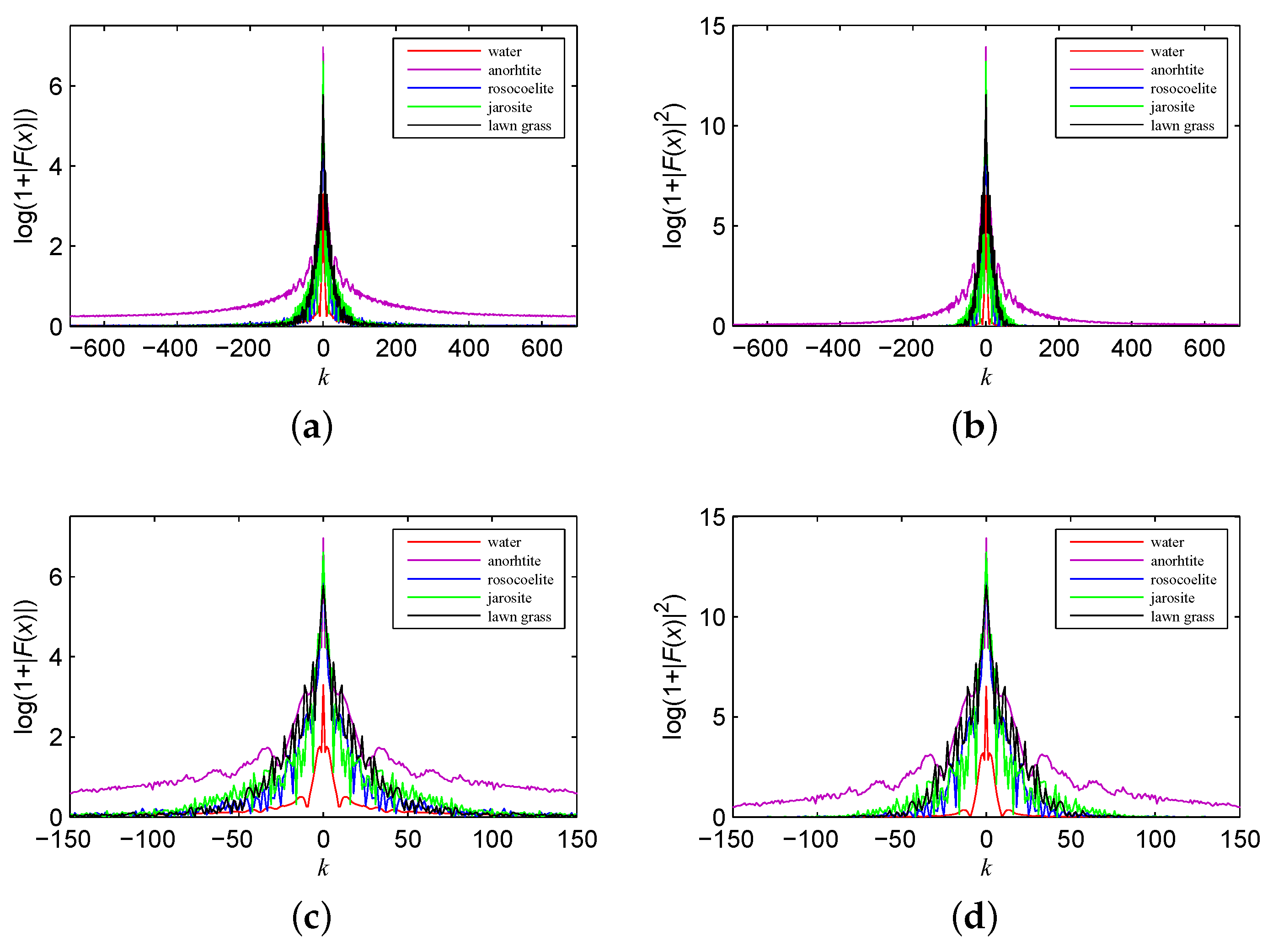
In Figure 4, we plot the frequency and power spectrum of all ground objects’ spectral signatures in the same figure to illustrate the differences. The value of the frequency and power spectrum of anorthite is significantly higher than that of the other ground objects, whereas the frequency and power spectrum of water is mostly lower than that of the others, especially around the DC component. As shown in Figure 4c,d, which shows the local region around the DC component, the crest and valley of the frequency and power spectrum appear at different locations for different ground objects. Therefore, we conclude that the frequency and power spectrum from the spectral signatures of different ground objects can be quite different from each other.
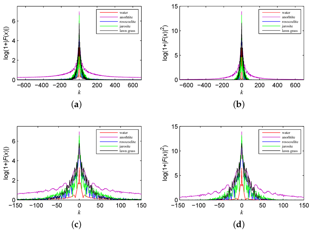
Figure 4.
Comparison of the (a) frequency and (b) power spectrum; details of the (c) frequency and (d) power spectrum.
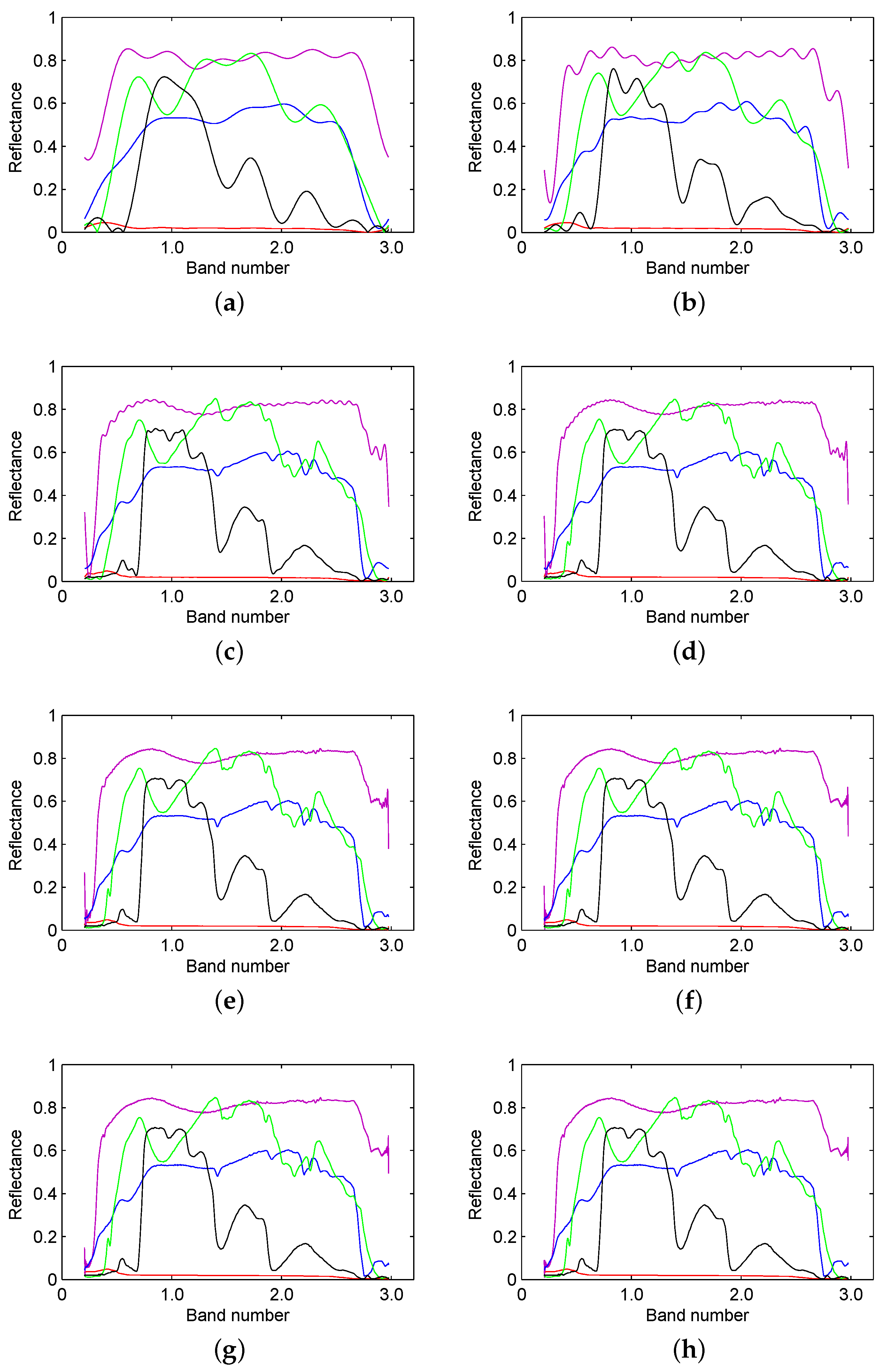
The work in [53,54] indicates that a certain amount of low frequencies is enough to describe the original spectral signature. Using Equation (7), the discrete signal can be expressed as the sum of harmonics, namely the frequency components. Therefore, in order to show the contribution from different frequency components, different ratios of harmonics are used to reconstruct the original signal. Figure 5 shows the reconstruction results from different ratios of the low frequency spectrum, namely 1%, 2%, 5%, 10%, 20%, 40%, 60% and 80%.
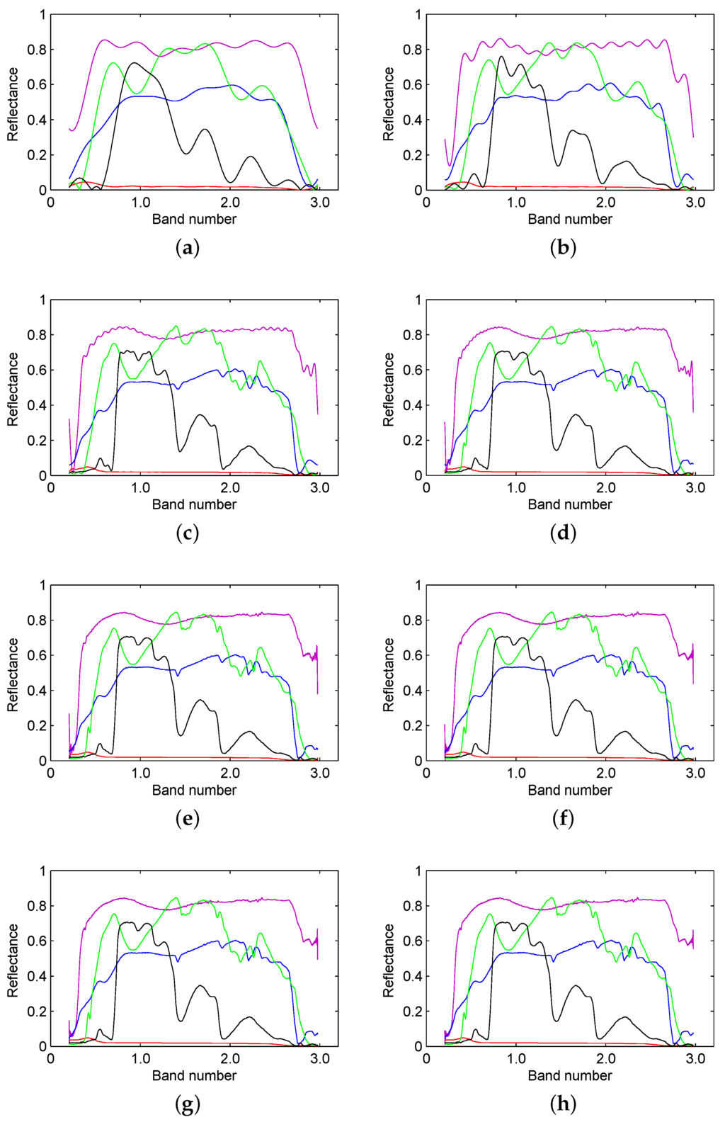
Figure 5.
Reconstruction results from (a) 1%; (b) 2%; (c) 5%; (d) 10%; (e) 20%; (f) 40%; (g) 60% and (h) 80% of the low frequency spectrum from the spectral signatures of water, anorthite, roscoelite, jarosite and lawn grass.
We can see that the reconstruction result becomes more similar to the original spectral signature as the ratio of the frequency spectrum (from low frequency to high frequency) increases. However, when this ratio is greater than 20%, the reconstruction is extremely close to the original signature. Therefore, a portion of the frequency spectrum can be used to describe the original spectral signature. We can use different ratios of the frequency spectrum to calculate the spectral similarity on the basis of the existing measure, in order to optimize the result.
2.3. Frequency-Based Measures from the Existing Measures
In this paper, we take the SAM, SID, SCM, ED, NED and SsS method for calculating the spectral similarity measures based on the frequency domain. Given the target and reference spectral curve (hyperspectral vector) and , each component and is a pixel of the i-th acquired at a particular wavelength . The SAM, SID, SCM, ED, NED and SsS methods are defined as follows:
(1) SAM:
(2) SID:
where the vector is the desired probability vector resulting from A; is the desired probability vector resulting from B.
(3) SCM:
where and are the mean values of the vectors A and B.
(4) ED:
(5) NED:
where and are the mean values of the vectors A and B.
(6) StS and SsS:
In our proposed measures, we take the frequency spectrum of the spectral signatures as the vector for calculating the existing measures, including the SAM, SID, SCM, ED, NED and SsS measures, and we call these measures frequency-based measures. Thus, F-SAM, F-SID, F-SCM, F-ED, F-NED and F-SsS are frequency-based measures from SAM, SID, SCM, ED, NED and SsS, respectively.
3. Experiment and Results
3.1. Dataset
3.1.1. AVIRIS Data on the Salinas Valley
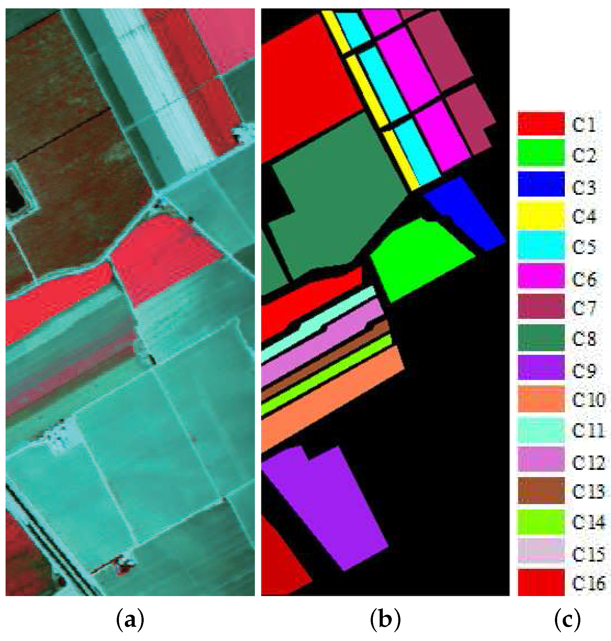
This dataset was acquired by the Airborne Visible/Infrared Imaging Spectrometer (AVIRIS) over Salinas Valley, California, in 1998. The original data contains 217 × 512 pixels and 220 spectral channels, which range from 0.4 to 2.45 m, covering the visible and infrared spectra. In our experiment, we discarded the 20 water absorption bands. The data were taken at a low altitude with a spatial resolution of 3.7 m. The dataset shown in Figure 6a, which is the false color composite image of Bands 18, 30 and 68, presents a vegetation scenario, including broccoli, corn, fallow, stubble, celery, vineyard and romaine lettuce. The main advantage of this dataset is that there is a ground truth map, shown in Figure 6b, including 16 land cover classes prepared at the time of image acquisition. The details of the land cover classes and sample number is listed in Table 1.

Figure 6.
(a) False color hyperspectral remote sensing image over the Salinas Valley (using Bands 68, 30 and 18); (b) ground truth of the labeled area with sixteen classes of land cover: Broccoli Green Weeds 1, Broccoli Green Weeds 2, fallow, fallow rough plow, fallow smooth, stubble, celery, grapes untrained, soil vineyard developed, corn senesced green weeds, romaine lettuce 4 wk, romaine lettuce 5 wk, romaine lettuce 6 wk, romaine lettuce 7 wk, vineyard untrained and vineyard vertical trellis. Note that wk here means week; (c) the legend of the classes for land cover of ground truth

Table 1.
Ground truth classes for the Salinas Valley scene and their respective sample number.
3.1.2. AVIRIS Data on the Indian Pines
The Indian Pines hyperspectral image is a dataset gathered by the AVIRIS sensor over the Indian Pines test site in northwestern Indiana and consists of 145 × 145 pixels with 224 bands. This dataset is commonly used for classification experiments because of the high similarity between spectral signatures of different classes and heavily mixed pixels. The data and ground truth map are shown in Figure 7a,b. The number of bands is initially reduced to 200 by removing water absorption bands and noisy bands. The original ground truth has actually 16 land cover classes, but some classes have a very small number of samples; therefore, 12 classes that have a higher number of samples were used in the experiment. The samples corresponding to each of these classes are shown in Table 2.
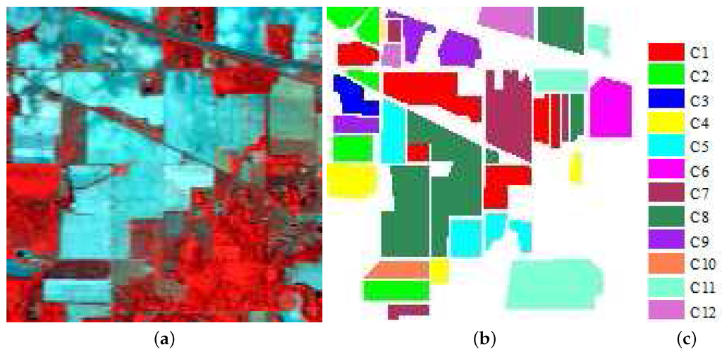
Figure 7.
(a) False color hyperspectral remote sensing image over the Indian Pines (using Bands 50, 27 and 17); (b) ground truth of the labeled area with twelve classes of land cover: corn-no till, corn-min till, corn, grass-pasture, grass-trees, hay-windrowed, soybean-no till, soybean-min till, soybean-clean, wheat, woods and buildings-grass-trees-drives; (c) the legend of the classes for land cover of ground truth

Table 2.
Ground truth classes for the Indian Pines scene and their respective sample number.
3.1.3. Hyperion Data on Botswana
The third experimental image is of Okavango Delta, Botswana, collected by the Hyperion sensor on EO-1. The hyperspectral data are 1476 × 256 pixels, with a spatial resolution of 30 m per pixel. We, here, took a sub-scene (1011 × 256 pixels) of this image as the experimental data. The number of spectral channels in the original data is 242 (with a spectral range between 0.5 and 2.5 m). The uncalibrated and noisy bands that cover water absorption features are removed, and only 145 bands remained for experiment. The ground truth information is available for partial areas of the scene, including 14 identified classes representing the land cover types, which are shown in Table 3. Figure 8 is the color composite image of the hyperspectral data.

Table 3.
Ground truth classes for the Botswana scene and their respective sample number.
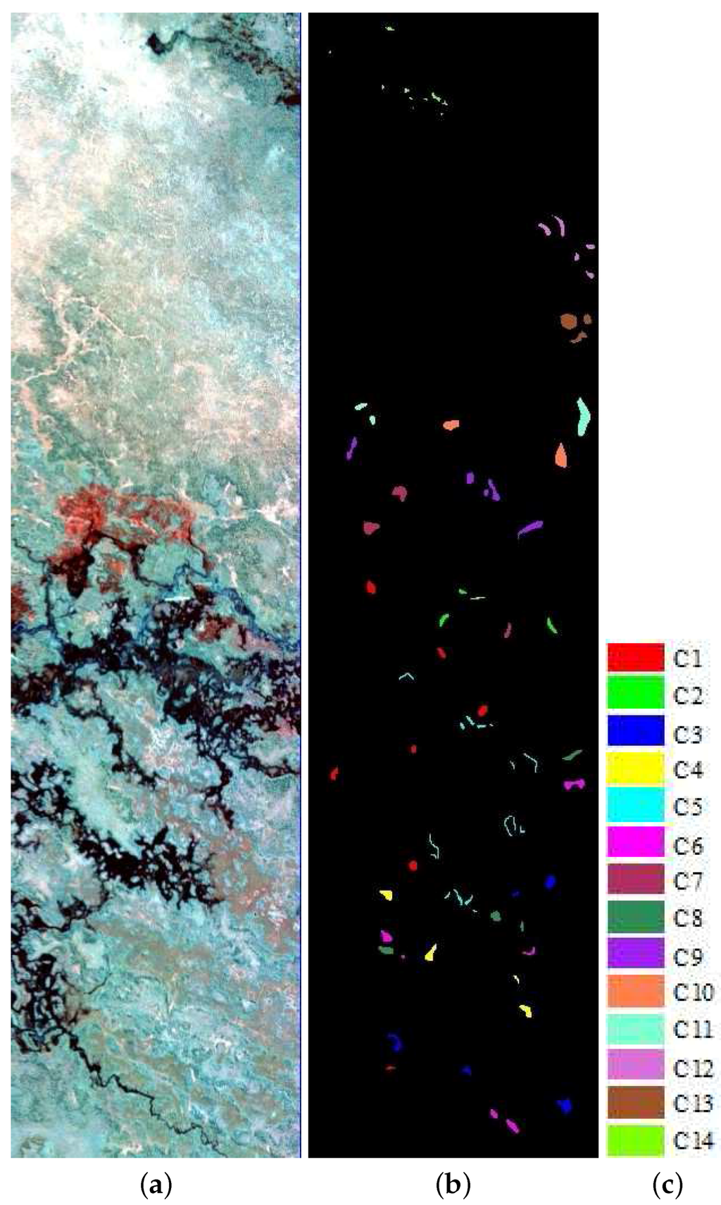
Figure 8.
(a) False color hyperspectral remote sensing image over Okavango Delta, Botswana (using Bands 149, 51 and 31); (b) ground truth of the labeled area with twelve classes of land cover: water, hippo grass, floodplain grasses 1, floodplain grasses 2, reeds 1, riparian, firescar 2, island interior, acacia woodlands, acacia shrublands, acacia grasslands, short mopane, mixed mopane and exposed soils; (c) the legend of the classes of land cover for ground truth
3.2. Experimental Setup
In these three experiments, the average of each class’s spectral signature from all labeled pixels in the ground truth data was taken as the reference spectral signature. In the class’s assignment of the unknown pixel, we first calculate the spectral similarity measure between this pixel and the reference spectral signature of all labeled class. The class’ label is assigned to the unknown pixel when the spectral similarity measure between this class and the unknown pixel is the highest value. We evaluated the classification accuracy of the proposed frequency-based measures, including F-SAM, F-SID, F-SCM, F-ED, F-NED and F-SsS (since the classification accuracies are extremely close between F-SsS and F-StS, we present only the accuracies of F-SsS.) and further compared these with the commonly-used measures, including SAM, SID, SCM, ED, NED and SsS. We first used the producer’s accuracy (PA), user’s accuracy (UA), overall accuracy (OA), average accuracy (AA) and Kappacoefficient to evaluate our proposed frequency-based measures and the commonly-used measures. Second, we calculated the OA, AA and Kappa coefficient of the classification results from different ratios of the frequency spectrum of spectral signatures. Furthermore, we obtained the optimal classification result and analyzed the relationship between the ratio of the frequency spectrum and the optimal result.
3.3. Experiment I: Salinas Valley Data
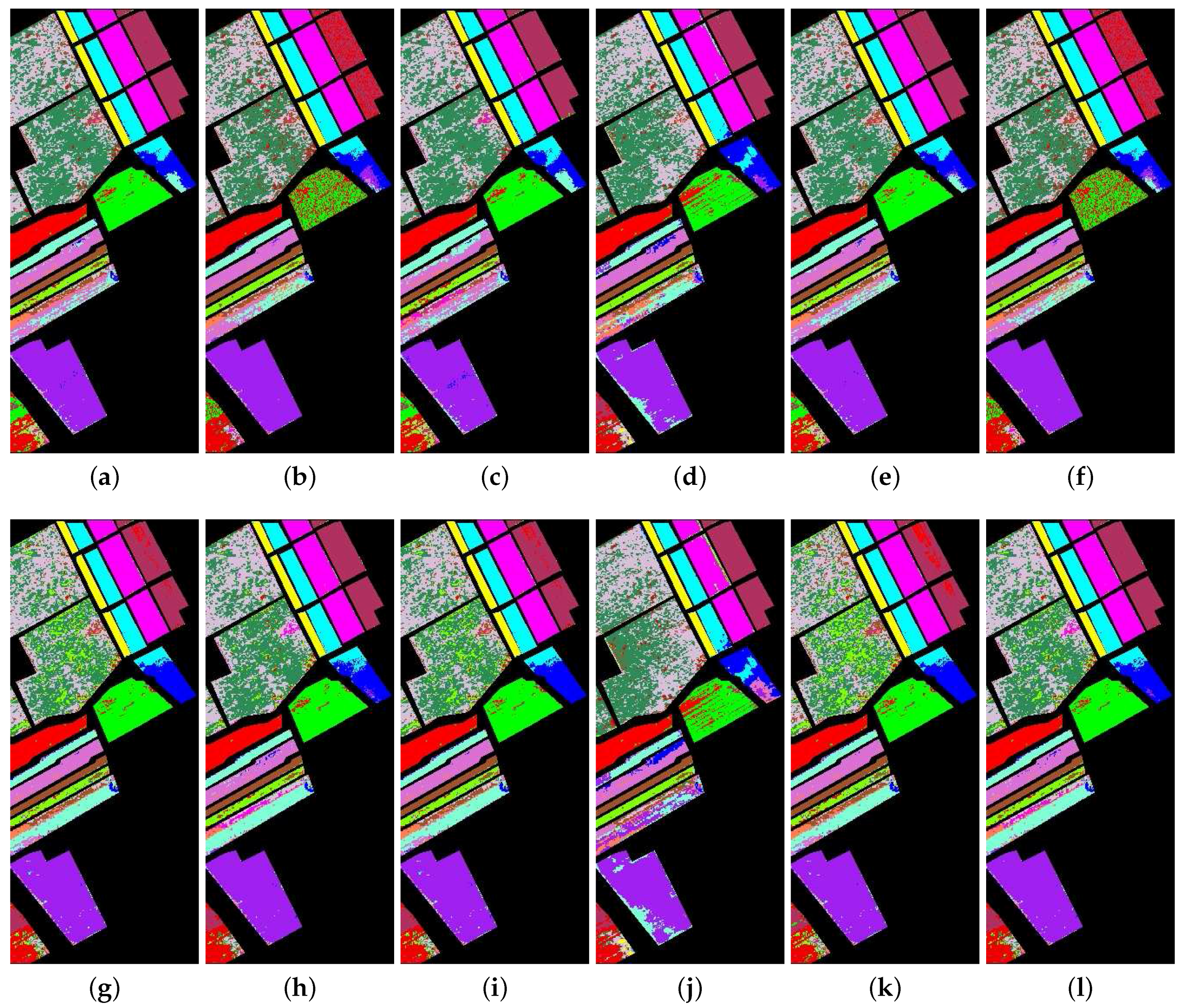
Figure 9 shows the classification map of these methods, including the SAM, SID, SCM, ED, NED, SsS, F-SAM, F-SID, F-SCM, F-ED, F-NED and F-SsS methods. We can see clearly that the classification results of C3, C8, C10, C15 and C16 show bad performance with all measures, especially the class of C10. The details of the classification accuracies, including the PA, UA, OA, AA and Kappa coefficient, are presented in Table 4.

Figure 9.
The classification map from the hyperspectral data on Salinas Valley. The first row is the result from the SAM, SID, SCM, ED, NED, and SsS methods, respectively; the second row is the result from the F-SAM, F-SID, F-SCM, F-ED, F-NED and F-SsS methods, respectively. (a) SAM; (b) SID; (c) SCM; (d) ED; (e) NED; (f) SsS; (g) F-SAM; (h) F-SID; (i) F-SCM; (j) F-ED; (k) F-NED; (l) F-SsS.

Table 4.
Class accuracies of the proposed frequency-based and existing methods over the Salinas Valley scene.
As shown from Table 4, it can be seen that F-SID reaches 76.79% OA, 81.85% AA and 0.7430 Kappa, all of which are higher than the accuracies of the other methods. The F-SsS and NED measures have better performance than the remaining measures. Meanwhile, although the OA and Kappa of the NED is slightly higher than that of the F-SsS, the AA of the NED is clearly lower than that of the F-SsS.
Furthermore, it is worth noting that two frequency-based measures, F-SID and F-SsS, obtain better results than their corresponding traditional measures, SID and SsS. SCM and F-SCM achieve close classification accuracies. The OA of F-SCM is slightly lower than that of the SCM, and the Kappa values are close to each other. However, the F-SCM’s AA is dramatically higher than that of SCM. F-SAM has worse performance than SAM, but the AA of F-SAM is close to that of the SAM. Finally, the accuracies of the F-ED and F-NED measures are worse than those of the ED and NED, respectively. Meanwhile, their accuracies have the worst performance of all of the frequency-based measures.
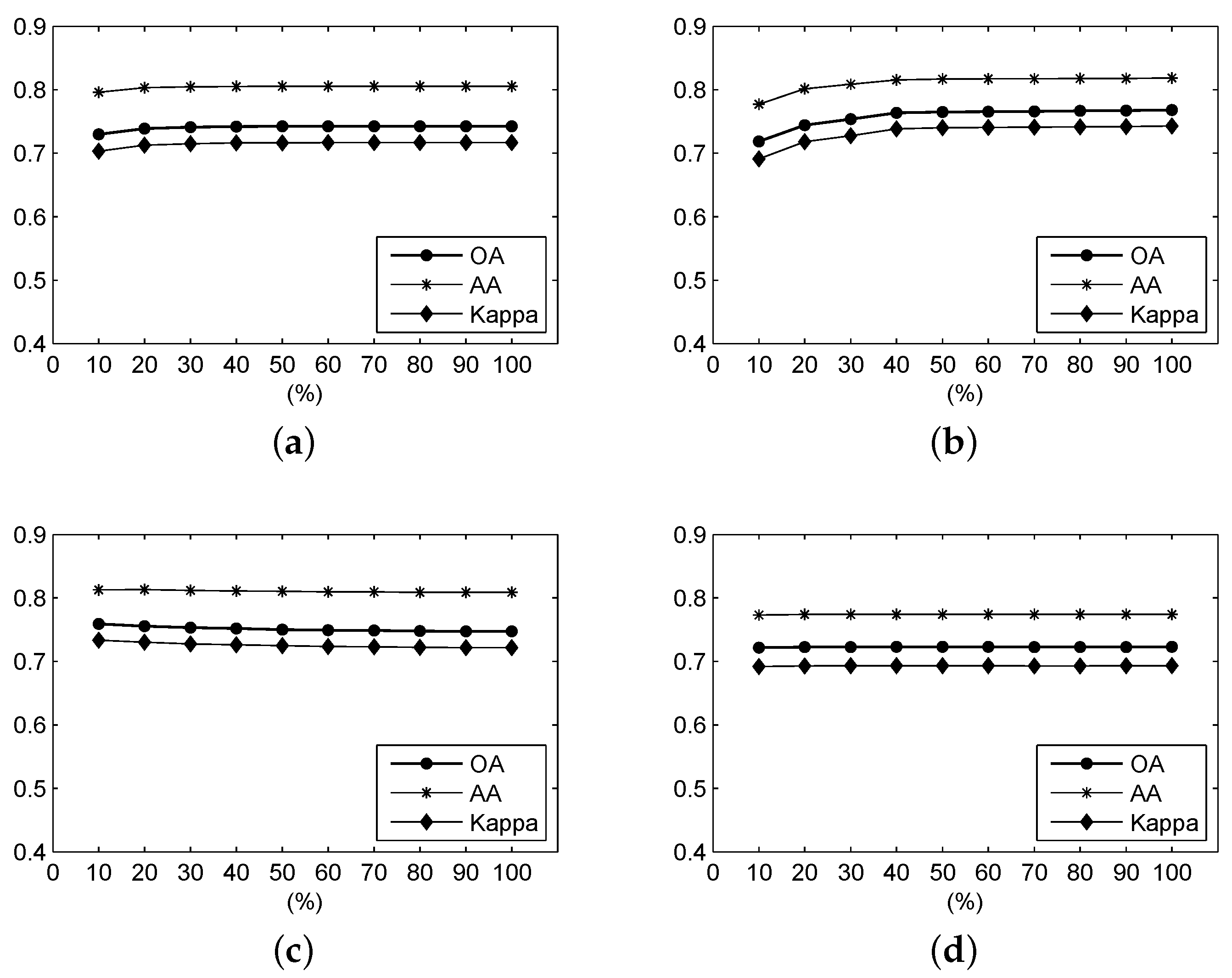
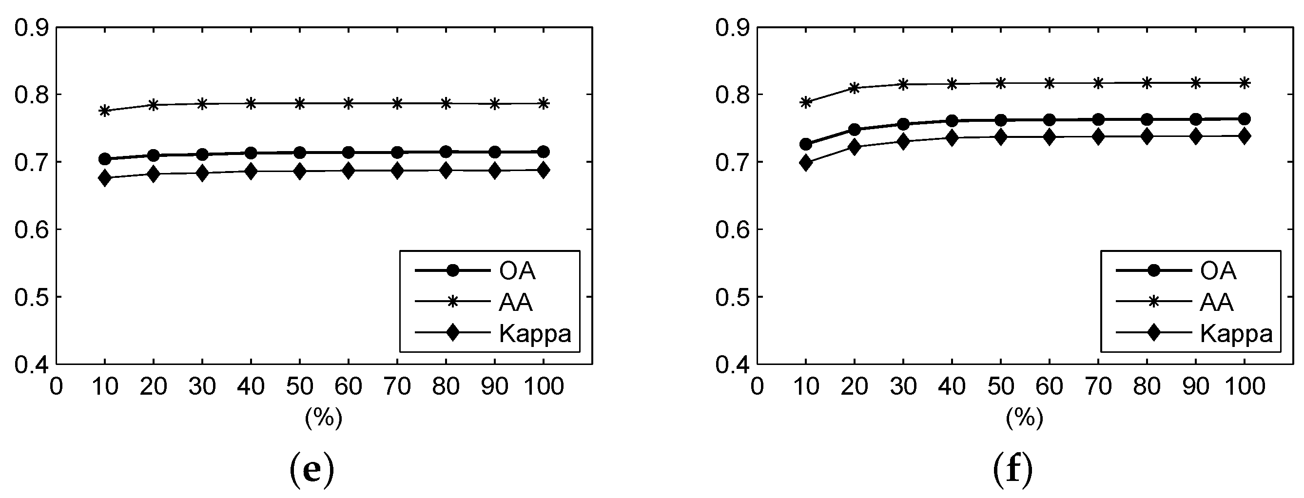
Figure 10 shows the OA, AA and Kappa coefficient of the classification results from different ratios of the frequency spectrum using frequency-based measures over the Salinas Valley scene. It can be seen that, for the F-SAM, F-SID, F-NED and F-SsS measures, when the ratio is larger than 0.2, the accuracies tend to be stable and exhibit higher values. For the F-SCM measure, the accuracies also tend to be stable when the ratio is over 0.2. However, these accuracies become lower than those with ratios lower than 0.2. The F-ED measure always exhibits very stable accuracies, which have been influenced by the ratio of the frequency spectrum.
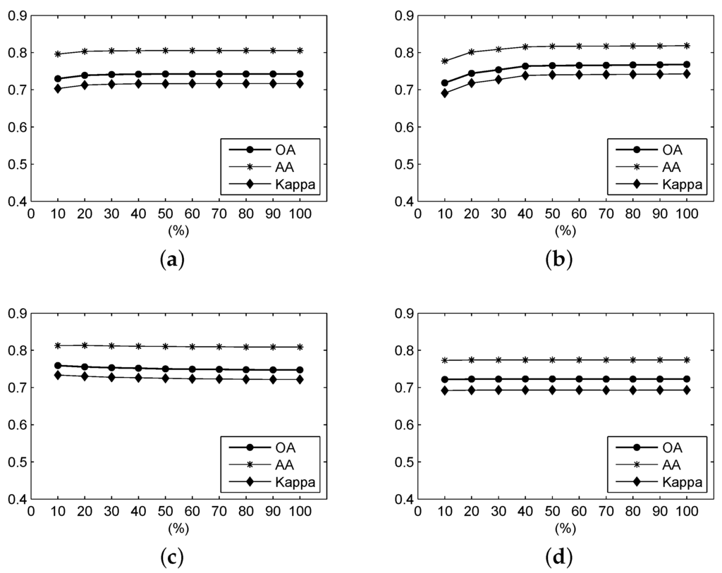

Figure 10.
For the Salinas Valley data, the OA, AA and Kappa coefficient of the classification result under different parameters using (a) F-SAM, (b) F-SID, (c) F-SCM, (d) F-ED, (e) F-NED, and (f) F-SsS.
Table 5 illustrates the optimal accuracy values and the corresponding ratios. We can clearly see that the optimal OA, AA and Kappa of F-SID and F-SsS still exhibit the best performance. The ratios of the optimal values from different measures are distinctly different. For the F-SID, F-SsS and F-NED, the ratio for optimization is close to 1.0. For F-SAM, the ratio is close to 0.8 or 0.9. The F-ED measure obtains the optimal values when the ratio is 0.5. The distinct difference is that the experimental result shows that F-SCM tends to have better performance when the ratio is close to 0.1.

Table 5.
Optimal accuracy values and the ratios of the frequency spectrum involved in the frequency-based measures in the experiment for Salinas Valley data.
3.4. Experiment II: Indian Pines Data
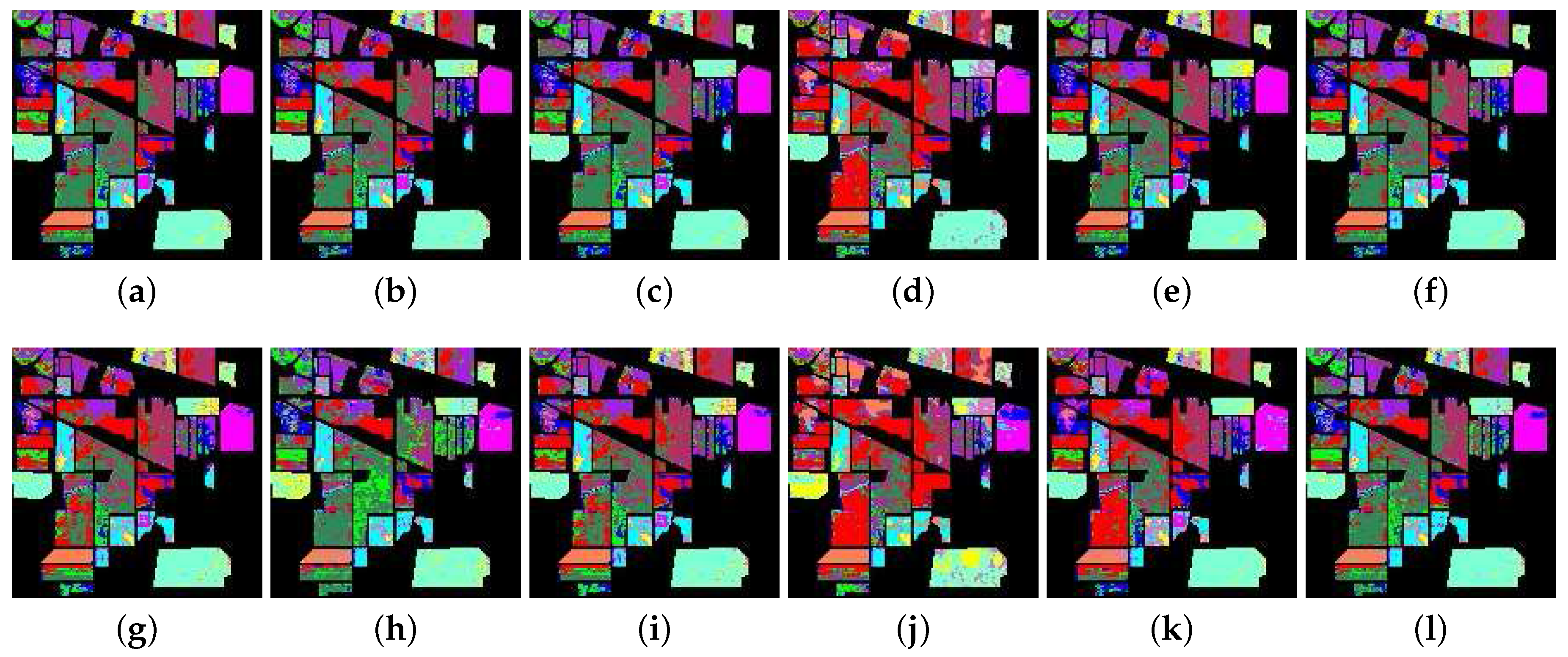
The classification maps on the Indian Pines data using these measures are shown in Figure 11. It is seen that the classification results of each class are not good based on all measures. In order to illustrate the difference of classification accuracies between each method in detail, the accuracies of PA, UA, OA, AA and the Kappa coefficient are shown in Table 6. We can see that the F-SsS has the highest values of OA (53%), AA (54.61%) and Kappa (0.4697) in all measures. For all frequency-based measures, only the F-SsS achieves better performance than the corresponding traditional measures. Furthermore, although the OA and Kappa of the F-SID are lower than those of the SID, the F-SID exhibits a significantly higher value of AA than that of the SID. For the F-SAM, F-SCM, F-ED and F-NED, the classification accuracies illustrate worse performance than the SAM, SCM, ED and NED.
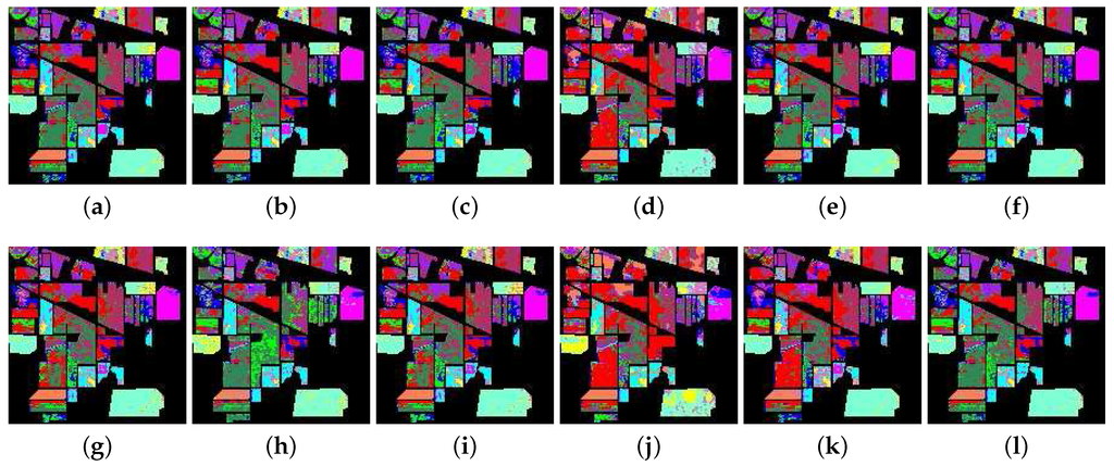
Figure 11.
The classification map from the hyperspectral data on Indian Pines. The first row is the result from the SAM, SID, SCM, ED, NED, and SsS methods, respectively; the second row is the result from the F-SAM, F-SID, F-SCM, F-ED, F-NED and F-SsS methods, respectively. (a) SAM; (b) SID; (c) SCM; (d) ED; (e) NED; (f) SsS; (g) F-SAM; (h) F-SID; (i) F-SCM; (j) F-ED; (k) F-NED; (l) F-SsS.

Table 6.
Class accuracies of the proposed and existing methods over the Indian Pines scene.
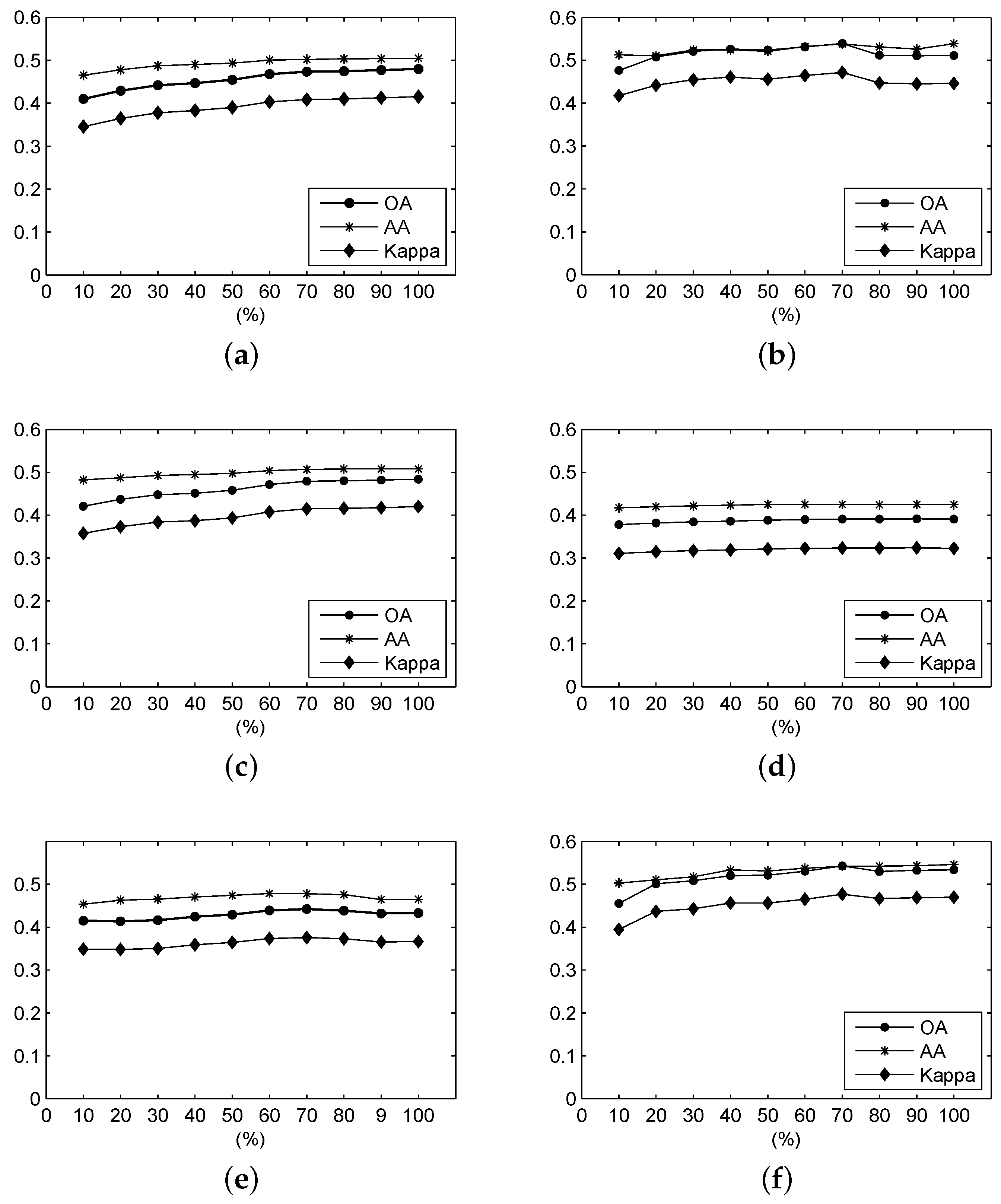
Figure 12 shows the OA, AA and Kappa coefficient of the classification results from different ratios of the frequency spectrum using frequency-based measures over the Indian Pines scene. It can be seen that these measures tend to obtain higher accuracies with increasing ratio. When the ratios of the F-SID and F-SsS measures exceed 0.7, there are slight decreases in the accuracies of the OA and Kappa. For their AA accuracies, the curve first increases, then decreases, and finally increases to the highest values at a ratio of 1.0. For the F-SAM and F-SCM, the accuracies rise with increasing ratio. The accuracies of OA, AA and Kappa fluctuate around 43.50%, 46.50% and 0.3660, respectively. The accuracies of the F-ED remain stable, without much fluctuation.
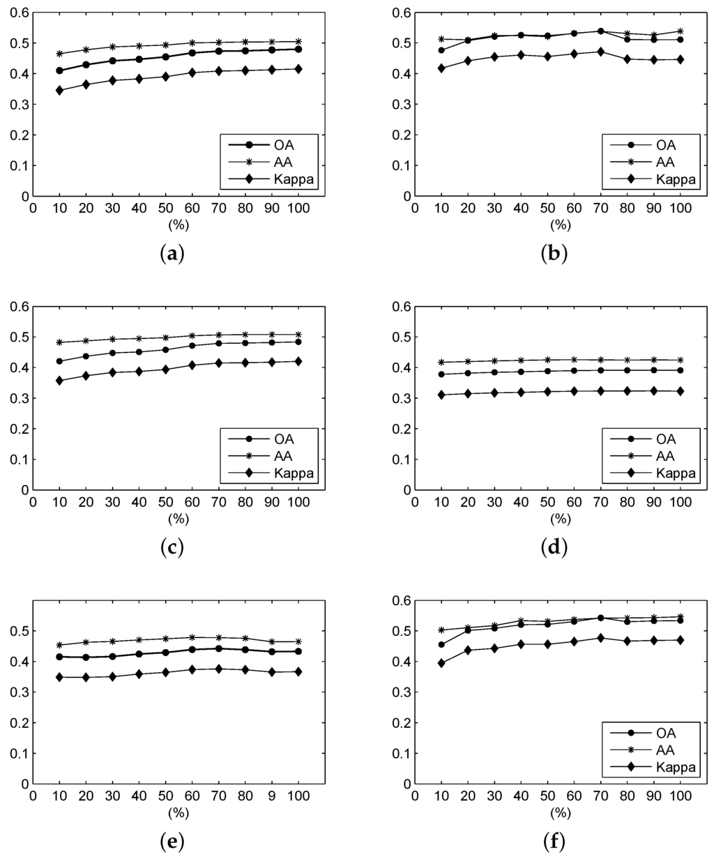
Figure 12.
For the Indian Pines data, the OA, AA and Kappa coefficient of the classification results under different parameters using (a) F-SAM; (b) F-SID; (c) F-SCM; (d) F-ED; (e) F-NED; and (f) F-SsS.
The optimal results are shown in Table 7. For the F-SAM and F-SCM, the optimal results are obtained when the ratio of the frequency spectrum of the spectral signature is 1.0. For the F-SID and F-SsS, the optimal results are obtained when this ratio is 0.7, even though the AA, when the ratio is 0.7, is lower than that when the ratio is 1.0. The OA, AA and Kappa coefficient of the optimal results for the F-SID are 53.89%, 53.83% and 0.4645, respectively. For the F-SsS, when the ratio is 0.7, the OA, AA and Kappa coefficient are 54.16%, 54.28% and 0.4769, respectively. We can see that the performance of the F-SID and F-SsS is distinguished. For the F-SAM and F-SCM, the optimal results are obtained at a ratio of 1.0. The F-NED obtains the best performance when the ratio is approximately 0.7. For the F-ED measure, the highest value of OA and Kappa are reached at a ratio of 0.9; the highest value of AA is also reached at a ratio of 0.9.

Table 7.
Optimal accuracy values and the corresponding ratio of the frequency spectrum involved in the experiment for the Indian Pines data.
3.5. Experiment III: Botswana Data
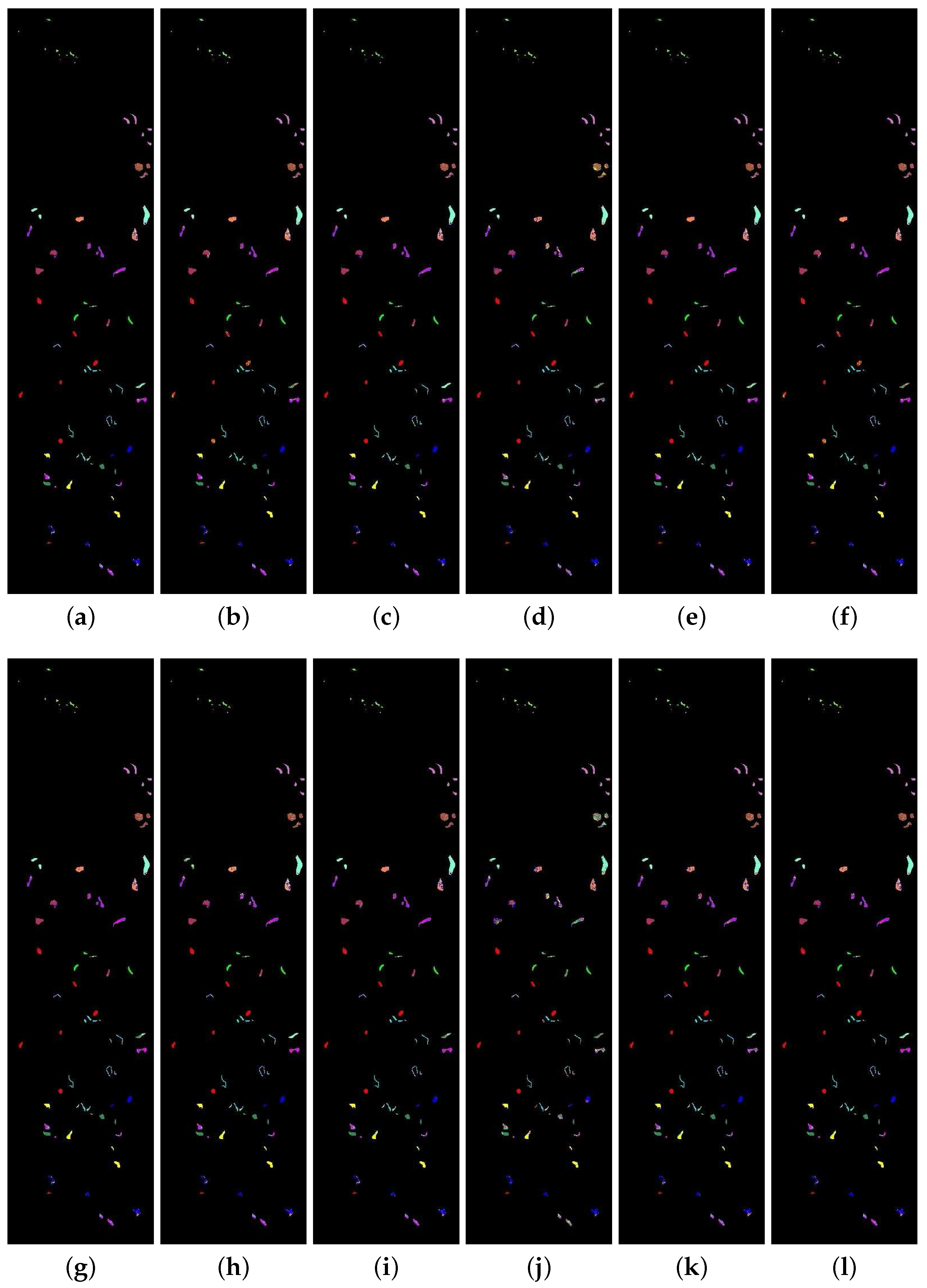
Figure 13 illustrates the classification map from different methods. The classification results generally have good performance in all measures. Only the class of C6 has distinctly bad performance. Table 8 exhibits the details of classification accuracies. Except for F-ED and F-NED, all frequency-based measures have excellent performance. The F-SsS, F-SAM, F-SCM and F-SID measures observably have better performance than the other measures. Meanwhile, the F-SsS exhibits the highest values of OA, AA and Kappa, at 84.17%, 85.27% and 0.8285, respectively. It is worth noting that, in this experiment, the F-SAM and F-SsS’s accuracies are much higher than the other measures. Furthermore, the F-ED and F-NED measures still have worse performance than the corresponding traditional measures.
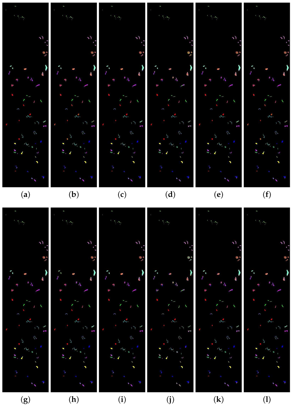
Figure 13.
The classification map from the hyperspectral data on Botswana. The first row is the result from the SAM, SID, SCM, ED, NED, and SsS methods, respectively; the second row is the result from the F-SAM, F-SID, F-SCM, F-ED, F-NED and F-SsS methods, respectively. (a) SAM; (b) SID; (c) SCM; (d) ED; (e) NED; (f) SsS; (g) F-SAM; (h) F-SID; (i) F-SCM; (j) F-ED; (k) F-NED; (l) F-SsS.

Table 8.
Class accuracies of the proposed and existing measures over the Botswana scene.
Figure 14 shows the OA, AA and Kappa coefficient of the classification results for different ratios of the frequency spectrum using frequency-based measures over the Botswana scene. We can see that, for the F-SID and F-SsS measures, the accuracies first increase distinctly and then decrease slightly. For the F-SAM and F-SCM, the accuracies increase when the ratio is close to 1.0, and the optimal result, shown in Table 9, is obtained when the ratio is 1.0. The fact that the tendency of the F-ED measure is not influenced by the ratio value is similar to the case of the Salinas Valley and Indian Pines scenes, even though the optimal result is also obtained at a ratio of 1.0. For the F-NED measure, the curve descends with increasing ratio.
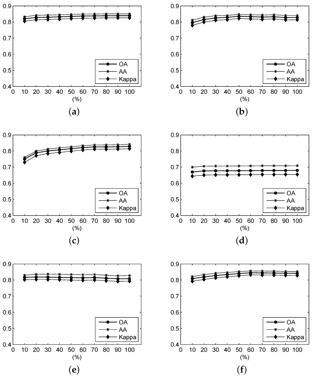
Figure 14.
For the Botswana data, the OA, AA and Kappa coefficient of the classification result under different parameters using (a) F-SAM; (b) F-SID; (c) F-SCM; (d) F-ED; (e) F-NED; and (f) F-SsS.

Table 9.
Optimal accuracy value and the ratio of the frequency spectrum involved in the frequency-based measures in the experiment for the Botswana data.
Table 9 illustrates that the F-SsS measure still has the best performance of all of the frequency-based measures. The optimal accuracies of the F-SID are close to those of the F-SAM measure, even though the accuracies of the F-SID measure are lower than those of the F-SAM measure. For the F-SAM and F-SCM, the optimal results are also obtained at ratios of 1.0. Although the F-ED also reaches its optimal result when the ratio is 1.0, the performances at other different ratio settings are very close the optimal result. For the F-NED, the highest accuracies are at ratios close to 0.2.
3.6. Discussion of the Results
As shown in Table 4, Table 6 and Table 8, the OA, AA and Kappa of the classification results of the three datasets illustrate that F-SsS and F-SID have better performance and more robust application than other measures. Especially, F-SsS always has the highest classification accuracies with the Indian Pines and Botswana data. It has the third best performance for the Salinas Valley data. However, the result is close to the second best performance (from the NED measure) and has distinctly higher AA accuracy than that of the NED measure. This indicates that the OA and Kappa could obtain higher values, if the test sample numbers for all classes were the same. The F-SID shows the best performance for the Salinas Valley data, but worse than that of the F-SsS for the other experimental data, according to Table 4 and Table 6. However,the performance shown in Table 6 and Table 9 indicate that its optimal result by choosing the fitting parameter is superior to the other measures except for the F-SsS. For example, although Table 6 shows that its accuracies, including OA, AA and Kappa, which are the fourth highest of all of the measures, are lower than the SID and SsS measures; the optimal OA (53.89%), AA (53.85%) and Kappa (0.4716) shown in Table 7 are much higher than those of the SID and SsS measures and are second only to the F-SsS.
For the F-SAM and F-SCM, the performance result is poor, even though the accuracies, such as OA, AA and Kappa, are sometimes higher than those of the SAM, SID, SCM, ED, NED and SsS, for example in the Botswana hyperspectral data. The F-ED and F-NED always present worse performance than the ED and NED in all three hyperspectral test data.
The ratio of the frequency spectrum involved in the proposed measure is used to optimize the classification accuracies and to analyze their robustness, as shown in Table 5, Table 7 and Table 9. The results illustrate that the F-SAM measure robustly achieves optimization when the ratio is close to 1.0. However, the F-SCM measures are labile. Although the optimal ratio in Table 5 is approximately 0.1, the optimal ratio in Table 7 and Table 9 is approximately 1.0. Figure 9, Figure 10 and Figure 11 show that the differences between the F-ED and F-NED measures’ accuracies are small, with the ratio varying in the three hyperspectral datasets, especially the F-ED. The reason is that the frequency energy of the high frequency spectrum is much less than that of the low frequency spectrum. The optimal performance of the F-SsS and F-SID measures is not robust compared to that of the F-SAM and F-ED; however, the tendency of the two measures indicates that their accuracies are close to the optimal accuracies when the ratio is 1.0.
4. Conclusions
In this paper, we have proposed several frequency-based spectral similarity measures based on commonly-used ones, including SAM, SID, SCM, ED, NED and SsS, by using the frequency spectrum of each pixel’s original spectral signature in the hyperspectral data. The frequency and power spectrum of five spectra in the USGS spectral library are analyzed, and the conclusion is that the frequency spectrum can be used to identify the difference among the land cover types. Thus, we proposed the F-SAM, F-SID, F-SCM, F-ED, F-NED and F-SsS using the frequency spectrum, according to the SAM, SID, SCM, ED, NED and SsS measures, respectively. In the proposed measures, a half length of the frequency spectrum is involved in the calculation because of the character of the symmetry around the DC component.
To evaluate the effectiveness of the proposed frequency-based measures, three hyperspectral datasets were adopted to compare these proposed measures with the existing ones, including the SAM, SID, SCM, ED, NED and SsS. A portion of the frequency spectrum arranged from low frequency to high frequency can be used to describe the original spectral signature. Furthermore, the region of low frequency around the DC component contains most of the frequency spectrum energy. Thus, the ratio of the frequency spectrum involved in the proposed measures is used to optimize the classification accuracies.
Conclusively, the experimental results show that the F-SsS is the best spectral similarity measure of all of the frequency-based measure. Furthermore, it exhibits higher robustness than the existing measures. The F-SID also exhibits good classification performance. Meanwhile, parameter choosing can prominently optimize the results with these two frequency-based measures. In summary, the experimental results suggest that the proposed F-SsS and F-SID measures are more beneficial, yielding more robust performance than other measures.
Acknowledgments
This work is supported by the National Natural Science Foundation of China (Grant No. 41401373), the Natural Science Foundation of Jiangsu Province, China (Grant No. BK20140842), and the Fundamental Research Funds for the Central Universities (Grant No. 2014B03514).
Author Contributions
Ke Wang had the original idea for the study and drafted the manuscript. Bin Yong contributed to the revision and polishing of the manuscript.
Conflicts of Interest
The authors declare that there is no conflicts of interest regarding the publication of this paper.
References
- Kaarna, A.; Zemcik, P.; Kalviainen, H.; Parkkinen, J. Compression of multispectral remote sensing images using clustering and spectral reduction. IEEE Trans. Geosci. Remote Sens. 2000, 38, 1588–1592. [Google Scholar] [CrossRef]
- Du, Q.; Fowler, J.E. Low-complexity principal component analysis for hyperspectral image compression. Int. J. High. Perform. Comput. Appl. 2008, 22, 438–448. [Google Scholar] [CrossRef]
- Tu, T.M. Unsupervised signature extraction and separation in hyperspectral images: A noise-adjusted fast independent component analysis approach. Opt. Eng. 2000, 39, 897–906. [Google Scholar] [CrossRef]
- Wang, J.; Chang, C.I. Independent component analysis-based dimensionality reduction with applications in hyperspectral image analysis. IEEE Trans. Geosci. Remote Sens. 2006, 44, 1586–1600. [Google Scholar] [CrossRef]
- Villa, A.; Benediktsson, J.A.; Chanussot, J.; Jutten, C. Hyperspectral image classification with independent component discriminant analysis. IEEE Trans. Geosci. Remote Sens. 2011, 49, 4865–4876. [Google Scholar] [CrossRef]
- Zhang, L.; Zhong, Y.; Huang, B.; Gong, J.; Li, P. On the impact of PCA dimension reduction for hyperspectral detection of difficult targets. IEEE Geosci. Remote Sens. 2005, 2, 192–195. [Google Scholar]
- Li, W.; Prasad, S.; Fowler, J.E.; Bruce, L.M. Locality-preserving dimensionality reduction and classification for hyperspectral image analysis. IEEE Trans. Geosci. Remote Sens. 2012, 50, 1185–1198. [Google Scholar] [CrossRef]
- Zhang, L.; Zhang, L.; Tao, D.; Huang, X. Tensor discriminative locality alignment for hyperspectral image spectral-spatial feature extraction. IEEE Trans. Geosci. Remote Sens. 2013, 51, 242–256. [Google Scholar] [CrossRef]
- Lee, J.; Woodyatt, A.; Berman, M. Enhancement of high spectralresolution remote-sensing data by a noise-adjusted principal components transform. IEEE Trans. Geosci. Remote Sens. 1990, 28, 295–304. [Google Scholar] [CrossRef]
- Amato, U.; Cavalli, R.M.; Palombo, A.; Pignatti, S.; Santini, F. Experimental approach to the selection of the components in the minimum noise fraction. IEEE Trans. Geosci. Remote Sens. 2009, 47, 153–160. [Google Scholar] [CrossRef]
- Ifarraguerri, A.; Chang, C.I. Unsupervised hyperspectral image analysis with projection pursuit. IEEE Trans. Geosci. Remote Sens. 2000, 38, 2529–2538. [Google Scholar]
- Jimenez, L.O.; Landgrebe, D.A. Hyperspectral data analysis and supervised feature reduction via projection pursuit. IEEE Trans. Geosci. Remote Sens. 1999, 37, 2653–2667. [Google Scholar] [CrossRef]
- Zhang, L.; Zhong, Y.; Huang, B.; Gong, J.; Li, P. Dimensionality reduction based on clonal selection for hyperspectral imagery. IEEE Trans. Geosci. Remote Sens. 2007, 45, 4172–4186. [Google Scholar] [CrossRef]
- Ye, Y.; Wu, Q.; Huang, J.Z.; Ng, M.K.; Li, X. Stratified sampling for feature subspace selection in random forests for high dimensional data. Pattern Recogn. 2013, 46, 769–787. [Google Scholar] [CrossRef]
- Dalponte, M.; Orka, H.O.; Gobakken, T.; Gianelle, D.; Nasset, E. Tree species classification in boreal forests with hyperspectral data. IEEE Trans. Geosci. Remote Sens. 2013, 51, 2632–2645. [Google Scholar] [CrossRef]
- Guo, B.; Gunn, S.R.; Damper, R.I. Band selection for hyperspectral image classication using mutual information. IEEE Geosci. Remote Sens. 2006, 3, 522–526. [Google Scholar] [CrossRef]
- Sotoca, J.; Pla, F. Hyperspectral data selection from mutual information between image bands. Lecture Notes Comput. Sci. 2006, 4109, 853–861. [Google Scholar]
- Marin, J.A.; Brockhaus, J.; Rolf, J.; Shine, J.; Schafer, J.; Balthazor, A. Assessing band selection and image classification techniques on HYDICE hyperspectral data. In Proceeedings of the IEEE International Conference on Systems, Man, and Cybernetics, Tokyo, Japan, 12–15 October 1999; Volume 2, pp. 1067–1072.
- Keshava, N. Distance metrics and band selection in hyperspectral processing with applications to material identification and spectral libraries. IEEE Trans. Geosci. Remote Sens. 2004, 42, 1552–1565. [Google Scholar] [CrossRef]
- Hoffbeck, J.P.; Landgrebe, D.A. Classification of remote sensing images having high spectral resolution. Remote Sens. Environ. 1996, 57, 119–126. [Google Scholar] [CrossRef]
- Jia, X.; Riehards, J.A. Segmented prineipal components transformation for efficient hyperspectral remote sensing image display and classification. IEEE Trans. Geosci. Remote Sens. 1999, 37, 538–542. [Google Scholar]
- Maghsoudi, Y.; Zoej, M.J.V.; Collins, M. Using class-based feature selection for the classification of hyperspectral data. Int. J. Remote Sens. 2011, 32, 4311–4326. [Google Scholar] [CrossRef]
- Cortes, C.; Vapnik, V. Support vector networks. Mach. Learn. 1995, 20, 273–297. [Google Scholar] [CrossRef]
- Mika, S.; Ratsch, G.; Scholkopf, B.; Smola, A.; Weston, J.; Muller, K.-R. Invariant feature extraction and classification in kernel spaces. In Advances in Neural Information Processing Systems; Kamel, M., Campilho, A., Eds.; MIT Press: Cambridge, MA, USA, 1999; pp. 526–532. [Google Scholar]
- Dundar, M.M.; Landgrebe, A. A cost-effective semisupervised classifier approach with kernels. IEEE Trans. Geosci. Remote Sens. 2004, 42, 264–270. [Google Scholar] [CrossRef]
- Ben-Hur, A.; Horn, D.; Siegelmann, H.; Vapnik, V. Support vector clustering. Mach. Learn. Res. 2001, 2, 125–137. [Google Scholar] [CrossRef]
- Ratsch, G.; Scholkopf, B.; Smola, A.; Mika, S.; Onoda, T.; Muller, K.-R. Robust ensemble learning. In Advances in Large Margin Classifiers; Smola, A., Bartlett, P., Scholkopf, B., Schuurmans, D., Eds.; MIT Press: Cambridge, MA, USA, 1999. [Google Scholar]
- Kawaguchi, S.; Nishii, R. Hyperspectral image classification by bootstrap AdaBoost with random decision stumps. IEEE Trans. Geosci. Remote Sens. 2007, 45, 3845–3851. [Google Scholar] [CrossRef]
- Camps-Valls, G.; Gomez-Chova, L.; Munoz-Mari, J.; Rojo-Alvarez, J.L.; Martinez-Ramon, M. Kernel-based framework for multitemporal and multisource remote sensing data classification and change detection. IEEE Trans. Geosci. Remote Sens. 2008, 46, 1822–1835. [Google Scholar] [CrossRef]
- Tarabalka, Y.; Fauvel, M.; Chanussot, J.; Benediktsson, J.A. SVM- and MRF-based method for accurate classification of hyperspectral images. IEEE Geosci. Remote Sens. 2010, 7, 736–740. [Google Scholar] [CrossRef]
- Fauvel, M.; Chanussot, J.; Benediktsson, J.A.; Villa, A. Parsimonious Mahalanobis kernel for the Classification of High Dimensional Data. Pattern Recogn. 2013, 46, 845–854. [Google Scholar] [CrossRef]
- Samat, A.; Du, P.; Liu, S.; Li, J.; Cheng, L. Ensemble extreme learning machines for hyperspectral image classification. IEEE J. Sel. Top. Appl. Earth Observ. Remote Sens. 2014, 7, 1060–1069. [Google Scholar] [CrossRef]
- Chan, J.C.W.; Paelinckx, D. Evaluation of Random Forest and Adaboost tree-based ensemble classification and spectral band selection for ecotope mapping using airborne hyperspectral imagery. Remote Sens. Environ. 2008, 112, 2999–3011. [Google Scholar] [CrossRef]
- Bernard, K.; Tarabalka, Y.; Angulo, J.; Chanussot, J.; Benediktsson, J.A.; Villa, A. Spectral-spatial classification of hyperspectral data based on a Stochastic minimum spanning forest approach. IEEE Trans. Image Process. 2012, 21, 2008–2012. [Google Scholar] [CrossRef] [PubMed]
- Tarabalka, Y.; Chanussot, J.; Benediktsson, J.A. Segmentation and classification of hyperspectral images using watershed transformation. Pattern Recognit. 2010, 43, 2367–2379. [Google Scholar] [CrossRef]
- Xue, Z.; Li, J.; Cheng, L.; Du, P. Spectral-spatial classification of hyperspectral data via morphological component analysis-based image separation. IEEE Trans. Geosci. Remote Sens. 2015, 53, 70–84. [Google Scholar]
- Li, J.; Bioucas-Dias, J.M.; Plaza, A. Spectral Cspatial hyperspectral image segmentation using subspace multinomial logistic regression and Markov random fields. IEEE Trans. Geosci. Remote Sens. 2012, 50, 192–195. [Google Scholar] [CrossRef]
- Li, J.; Bioucas-Dias, J.M.; Plaza, A. Spectral-spatial classification of hyperspectral data using loopy belief propagation and active learning. IEEE Trans. Geosci. Remote Sens. 2013, 51, 844–856. [Google Scholar] [CrossRef]
- Camps-Valls, G.; Marsheva, T.V.B.; Zhou, D.Y. Semi-supervised graph-based hyperspectral image classification. IEEE Trans. Geosci. Remote Sens. 2007, 45, 3044–3054. [Google Scholar] [CrossRef]
- Camps-Valls, G.; Marsheva, T.V.B.; Zhou, D.Y. A graph-based classification method for hyperspectral images. IEEE Trans. Geosci. Remote Sens. 2013, 51, 803–817. [Google Scholar]
- Soltani-Farani, A.; Rabiee, H.R.; Hosseini, S.A. Spatial-aware dictionary learning for hyperspectral image classification. IEEE Trans. Med. Imaging 2015, 53, 527–541. [Google Scholar] [CrossRef]
- Sun, X.; Nasrabadi, N.M.; Tran, T.D. Task-driven dictionary learning for hyperspectral image classification with structured sparsity constraints. IEEE Trans. Geosci. Remote Sens. 2015, 53, 4457–4471. [Google Scholar] [CrossRef]
- Bazi, Y.; Melgani, F. Gaussian process approach to remote sensing image classification. IEEE Trans. Geosci. Remote Sens. 2010, 48, 186–197. [Google Scholar] [CrossRef]
- Richards, J.A.; Jia, X. Remote Sensing Digital Image Analysis, an Introduction; Springer: Berlin, Germany, 1999. [Google Scholar]
- Robila, S.A.; Gershman, A. Spectral matching accuracy in processing hyperspectral data. In Proceedings of the IEEE International Symposium on Signals, Circuits and Systems, ISSCS 2005, Iasi, Romania, 14–15 July 2005; Volume 1, pp. 165–166.
- Kruse, F.A.; Lefkoff, A.B.; Boardman, J.W.; Heidebrecht, K.B.; Shapiro, A.T.; Barloon, P.J.; Goetz, A.F.H. The spectral image processing system (SIPS)–Interactive visualization and analysis of imaging spectrometer data. Remote Sens. Environ. 1993, 44, 145–163. [Google Scholar] [CrossRef]
- Yang, C.H.; Everitt, J.H. Using spectral distance, spectral angle and plant abundance derived from hyperspectral imagery to characterize crop yield variation. Precis. Agric. 2012, 13, 62–75. [Google Scholar] [CrossRef]
- Chang, C.I. An information-theoretic approach to spectral variability, similarity, and discrimination for hyperspectral image analysis. IEEE Trans. Inform. Theory 2000, 46, 1927–1932. [Google Scholar] [CrossRef]
- De Carvalho, O.A., Jr.; Meneses, P.R. Spectral correlation mapper (SCM): An improvement on the spectral angle mapper (SAM). In Proceeedings of the Summaries of the 9th JPL Airborne Earth Science Workshop, Pasadena, American, 23–25 February 2000; Volume 2, pp. 65–74.
- Du, Y.; Chang, C.I.; Ren, H.; DceAmico, F.M.; Jensen, J.O. New hyperspectral discrimination measure for spectral characterization. Opt. Eng. 2004, 43, 1777–1786. [Google Scholar]
- Salgado, B.P.G.; Ponomaryov, V. Feature extraction-selection scheme for hyperspectral image classification using Fourier transform and Jeffries-Matusita distance. Lecture Notes Comput. Sci. 2015, 9414, 337–348. [Google Scholar]
- Hsu, S.M.; Burke, H.H.K. Multisensor fusion with hyperspectral imaging Data: Detection and classification. Lincoln Lab. J. 2003, 14, 145–159. [Google Scholar]
- Wang, K.; Gu, X.; Yu, T.; Meng, Q.; Zhao, L.; Feng, L. Classification of hyperspectral remote sensing images using frequency spectrum similarity. Sci. China Technol. Sci. 2013, 56, 980–988. [Google Scholar] [CrossRef]
- Wang, K.; Yong, B.; Gu, X.; Xiao, P.; Zhang, X. Spectral similarity measure using frequency spectrum for hyperspectral image classification. IEEE Geosci. Remote Sens. 2015, 12, 130–134. [Google Scholar] [CrossRef]
- Fourier, J. La Theorie Analytique De La Chaleur; Firmin Didot: Paris, France, 1822. [Google Scholar]
© 2016 by the authors; licensee MDPI, Basel, Switzerland. This article is an open access article distributed under the terms and conditions of the Creative Commons Attribution (CC-BY) license (http://creativecommons.org/licenses/by/4.0/).

