AVHRR GAC SST Reanalysis Version 1 (RAN1)

Abstract

In response to its users’ needs, the National Oceanic and Atmospheric Administration (NOAA) initiated reanalysis (RAN) of the Advanced Very High Resolution Radiometer (AVHRR) Global Area Coverage (GAC; 4 km) sea surface temperature (SST) data employing its Advanced Clear Sky Processor for Oceans (ACSPO) retrieval system. Initially, AVHRR/3 data from five NOAA and two Metop satellites from 2002 to 2015 have been reprocessed. The derived SSTs have been matched up with two reference SSTs—the quality controlled in situ SSTs from the NOAA in situ Quality Monitor (iQuam) and the Canadian Meteorological Centre (CMC) L4 SST analysis—and analyzed in the NOAA SST Quality Monitor (SQUAM) online system. The corresponding clear-sky ocean brightness temperatures (BT) in AVHRR bands 3b, 4 and 5 (centered at 3.7, 11, and 12 µm, respectively) have been compared with the Community Radiative Transfer Model simulations in another NOAA online system, Monitoring of Infrared Clear-sky Radiances over Ocean for SST (MICROS). For some AVHRRs, the time series of “AVHRR minus reference” SSTs and “observed minus model” BTs are unstable and inconsistent, with artifacts in the SSTs and BTs strongly correlated. In the official “Reanalysis version 1” (RAN1), data from only five platforms—two midmorning (NOAA-17 and Metop-A) and three afternoon (NOAA-16, -18 and -19)—were included during the most stable periods of their operations. The stability of the SST time series was further improved using variable regression SST coefficients, similarly to how it was done in the NOAA/NASA Pathfinder version 5.2 (PFV5.2) dataset. For data assimilation applications, especially those blending satellite and in situ SSTs, we recommend bias-correcting the RAN1 SSTs using the newly developed sensor-specific error statistics (SSES), which are reported in the product files. Relative performance of RAN1 and PFV5.2 SSTs is discussed. Work is underway to improve the calibration of AVHRR/3s and extend RAN time series, initially back to the mid-1990s and later to the early 1980s.

1. Introduction

The Advanced Clear Sky Processor for Ocean (ACSPO) is the NOAA sea surface temperature (SST) retrieval system [1,2,3,4]. It is currently employed to produce operational polar SST products from several Advanced Very High Resolution Radiometers (AVHRRs) onboard the US’ NOAA and European Organization for the Exploitation of Meteorological Satellites (EUMETSAT) Metop satellites, and from the new Visible Infrared Imager Radiometer Suite (VIIRS) onboard the Suomi National Polar-orbiting Partnership (S-NPP) platform. Two experimental SST products—from the Advanced Himawari Imager (AHI) onboard the geostationary Japanese Meteorological Agency (JMA) Himawari-8 satellite, and from two Moderate Resolution Imaging Spectroradiometers (MODIS) onboard the NASA Terra and Aqua polar satellites—are also produced at the NOAA Center for Satellite Applications and Research (STAR).

This study focuses on the AVHRR Global Area Coverage (GAC) data. Recall that the AVHRR native resolution is ~1 km at nadir and degrades to ~7 km at swath edge. The Metop satellites have enough storage onboard to save the Full Resolution Area Coverage (FRAC) data and downlink them to the ground, whereas the data onboard the NOAA satellites are sub-sampled to a Global Area Coverage (GAC) format, and transmitted to the ground with a nominal ~4 km resolution at nadir. In addition to the FRAC format, Metop data can be also sub-sampled to a GAC resolution on the ground, for those users interested in reduced volume Metop AVHRR data in the NOAA GAC format.

One of the main SST users at NOAA is the Coral Reef Watch (CRW) Program, which uses the geo-polar blended (GPB) Level 4 (L4) SST product produced by blending polar (Metop-B AVHRR and S-NPP VIIRS) and geostationary (NOAA GOES, EUMETSAT Meteosat and JMA Himawari-8) Level 2 (L2) SST products ([5], and references therein). The CRW monitoring is based on SST anomalies, i.e., deviations of the GPB SSTs from a reference state (SST climatology). Presently, the time series of the GPB SST are too short to derive a meaningful reference state and AVHRR Pathfinder (PF) SST climatology [6,7,8] is employed instead, with an empirical bias correction.

Despite the bias correction, the GPB and bias-corrected PF products remain inconsistent, and NOAA initiated a pilot project to generate a long-term record of GPB L4 SST, suitable for producing an initial climatology. This in turn requires reprocessing of the corresponding polar and geostationary L2 SST records. This paper documents the ACSPO AVHRR GAC Reanalysis version 1 (hereafter, “RAN1”). The start time requested by the CRW Team (January 2004) was deliberately extended in RAN1 to August 2002, the time when SST data from the first mid-morning NOAA-17 satellite became available. Below, the RAN1 dataset is documented, along with its major challenges, limitations, adopted tradeoffs, and the future work to resolve those. Both daytime and nighttime data are reported in RAN1, but the discussion is limited to nighttime SSTs only, as requested by the current users.

2. Data, Methodology, Results

The focus of RAN1 are the AVHRR/3 sensors flown onboard the NOAA-KLMNN’ (NOAA-15 to 19) and Metop series. Relevant to SST applications, the major improvement over the AVHRR/2 (the first AVHRR with a split-window capability, suitable for multi-channel SST retrievals) was installation of a larger external sun shield to the scan motor housing on NOAA satellites, to reduce sunlight impingement on the sensor and to stabilize its thermal regime, which in turn improved the quality and stability of its IR calibration. The AVHRR/3 GAC data analyzed in this study are summarized in

Table 1. The Advanced Very High Resolution Radiometer (AVHRR)/3 Global Area Coverage (GAC) data analyzed in this study and a subset used in Reanalysis version 1 (RAN1). The Equator Crossing Time (ECT) of the nighttime satellite pass, and the year from which static sea surface temperature (SST) regression coefficients were derived, are also shown.

Satellite	Type of Orbit	Night ECT	L1b Data Available	Used in RAN1	Static SST Coefficients
NOAA-16	Afternoon/PM	2:00 A.M.	29 December 2000–6 June 2014	30 August 2002–6 June 2005	2003
NOAA-18	Afternoon/PM	2:00 A.M.	20 May 2005–present	7 June 2005–21 February 2009	2006
NOAA-19	Afternoon/PM	2:00 A.M.	6 February 2009–present	22 February 2009–present	2010
NOAA-15	Morning/AM	7:30 P.M.	26 October 1998–present	Not used	2003
NOAA-17	Midmorning/AM	10:00 P.M.	25 June 2002–10 April 2013	30 August 2002–14 December 2006	2003
Metop-A	Midmorning/AM	9:30 P.M.	30 October 2006–present	15 December 2006–present	2007
Metop-B	Midmorning/AM	9:30 P.M.	24 September 2012–present	Not used	2013

. Note that the AVHRR L1b data are available from the NOAA Comprehensive Large Array-data Stewardship System (CLASS; www.class.noaa.gov). This study uses a copy of this data available at the NOAA Center for Satellite Applications and Research (STAR) Central Data Repository on a spinning disk.

2.1. ACSPO Processing

The AVHRR L1b GAC orbital files are first aggregated into 1-hr non-overlapping granules. The ACSPO processing is organized into three major interleaved blocks: (1) forward radiance calculations using the NOAA Community Radiative Transfer Model (CRTM), with the Canadian Meteorological Center (CMC) L4 SST analysis [9] and the National Centers for Environmental Prediction (NCEP) Global Forecast System (GFS; www.emc.ncep.noaa.gov/index.php?branch=GFS) first guess fields as inputs [2]; (2) identification of clear-sky ocean pixels suitable for SST retrievals [1]; and (3) calculation of SST using the regression equations [3,4]. The following Multi-Channel SST (MCSST; nighttime) and Non-Linear SST (NLSST; daytime) equations are used in RAN1:

MCSST (Night; Solar Zenith Angle, SZA > 90°)

$$T_S=a_o+a_1{T}_{3.7}+a_2{T}_{3.7}S+a_3\left(T_{11}-T_{12}\right)+a_4\left(T_{11}-T_{12}\right)S+a_{5}S$$

(1)

NLSST (Day; SZA ≤ 90°)

$$T_S=b_o+b_1{T}_{11}+b_2{T}_{11}S+b_3\left(T_{11}-T_{12}\right)+b_4\left(T_{11}-T_{12}\right)\left(T_o-273.15\right)+b_5\left(T_{11}-T_{12}\right)S+b_{6}S$$

(2)

Here, T_3.7, T₁₁ and T₁₂ are brightness temperatures (BTs) observed in AVHRR bands centered at 3.7, 11 and 12 µm, respectively; S = sec(VZA) − 1, VZA is the view zenith angle, and T_o is the first guess CMC L4 SST interpolated in space to the retrieval pixel. Only highest quality level (QL = 5) ACSPO data are used.

2.2. SSTs Derived Using Static Regression Coefficients

The static SST regression coefficients were calculated using one full calendar year from 1 January to 31 December (of the year following 2002 or the year in which the satellite was launched; shown in the 5th column of Table 1). ACSPO SSTs, T_S, and BTs have been matched up with quality controlled in situ SSTs, T_{in situ}, from the drifting and tropical moored buoys in the NOAA in situ Quality Monitor system (iQuam; www.star.nesdis.noaa.gov/sod/sst/iquam/, [10]), by selecting the closest in space ACSPO SST pixel within (10 km, 2 hr) of T_{in situ}. The SST coefficients have been first calculated using all matchups, and then recalculated excluding outlier points in which the AVHRR SST deviated from the in situ SST by more than 4 global standard deviations (SD) of ΔT_S = T_S − T_{in situ}. (This exclusion had a very minor impact on the SST coefficients.) The static coefficients have been applied to the full record of all seven AVHRRs. For routine validation in the NOAA SST Quality Monitor system (SQUAM; www.star.nesdis.noaa.gov/sod/sst/squam/, [11]), the ACSPO SSTs were matched up with iQuam in situ SSTs using the same matchup criteria, except the space-time window was relaxed to (20 km, 4 hr), which is currently the standard setting in SQUAM. One anonymous reviewer of this paper suggested reducing the time window to ±2 or even ±1 hr, if enough collocations are available. Rerunning the validation analyses is possible but proper selection of the new parameters should be based on sensitivity analyses, which are currently underway but were challenging to complete in the limited time allocated for the revision. Note also that the diurnal changes are relatively small at night, and if anything, all validation statistics shown in this study should only improve if smaller windows are used.

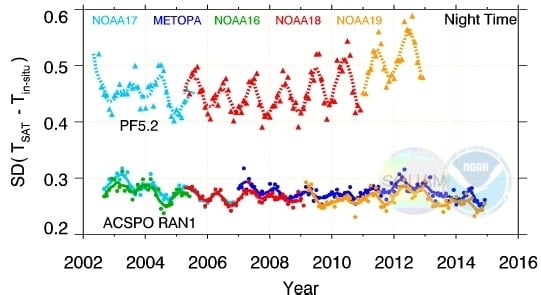
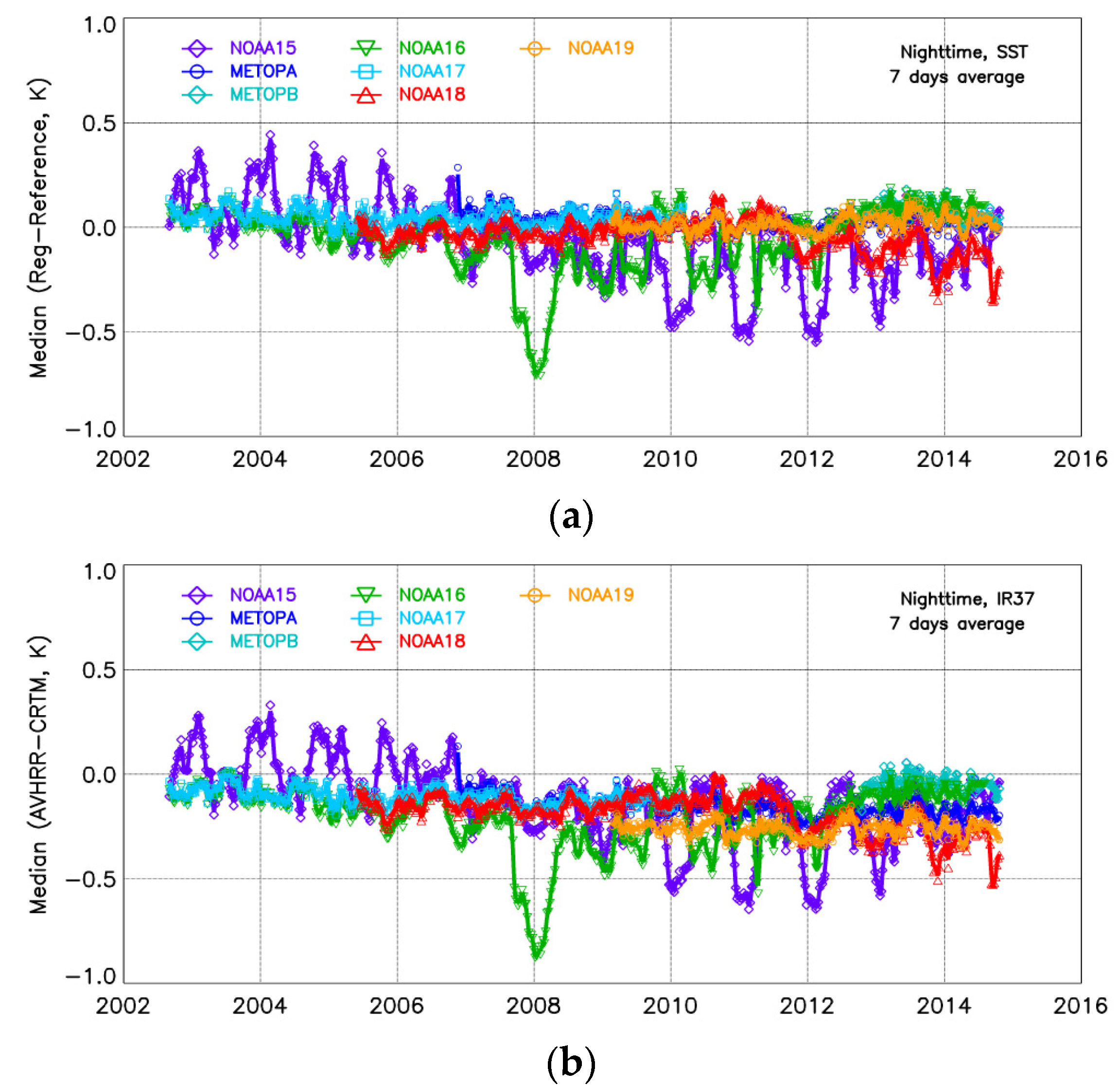
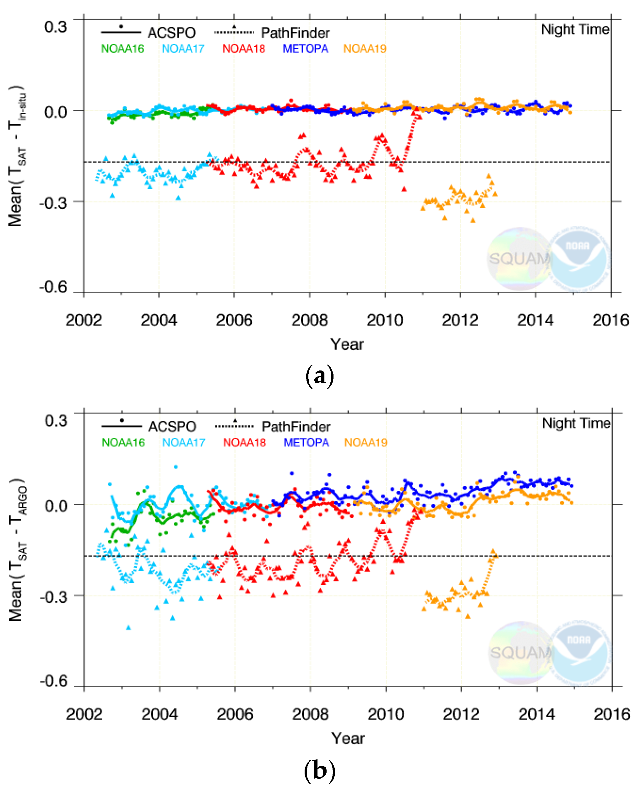
The time series of nighttime mean ΔT_S are shown in Figure 1a as they appear in the NOAA SQUAM system. For some platforms, the derived SSTs are stable and close to in situ SSTs, for the full time of their operation (e.g., Metop-A and -B, and NOAA-17 and -19). For some others, the initial periods of stability alternate with periods of uncontrolled variations (e.g., NOAA-16 and -18). And yet for some others, the SSTs are unstable for the full period from 2002 to present (e.g., NOAA-15).

2.3. The Root Cause of the Unstable SSTs

To attribute the anomalous SST behavior in Figure 1, another NOAA monitoring system is employed. Similarly to SQUAM, the MICROS system (www.star.nesdis.noaa.gov/sod/sst/micros/, [12]) monitors deviations of regression SST, T_S, from the first guess L4 CMC SST, T_L4: ΔT_S = T_S − T_L4. In addition, it also monitors deviations of the “observed” AVHRR BTs, T_O, from their “model” counterparts, T_M: ΔT_B = T_O − T_M, in three AVHRR bands 3b, 4, and 5. The time series of ΔT_S and ΔT_B in band 3b (which contributes most to the nighttime SST) corresponding to Figure 1a are shown in Figure 2a,b, respectively, as they appear in MICROS.

The two ΔT_S’s in Figure 1a and Figure 2a are in close agreement. This is expected because the CMC L4, ACSPO AVHRR L2, and iQuam in situ data all characterize the same “true SST” state. However, they do it differently. In particular, the global gap-free CMC L4 SST is produced by anchoring several infrared and microwave satellite SST products to in situ SST and blending them together. (Note that the ACSPO AVHRR and iQuam in situ SSTs have not been assimilated in the CMC L4 used here.) Also, Figure 2a is based on the full global ACSPO retrieval domain, whereas Figure 1a uses only its relatively small (<1/1000) in situ matchup sub-sample. As a result, the time series of (T_S − T_L4) are less noisy compared to (T_S − T_{in situ}), because the day-to-day noise is suppressed more efficiently in the L4 matchups than in the in situ matchups, due to the three orders of magnitude larger matchup samples.

Figure 2b shows ΔT_B’s in band 3b corresponding to the ΔT_S’s in Figure 2a. The two time series strongly correlate, suggesting that the major reason for the SST artifacts in Figure 1a and Figure 2a are the unstable AVHRR BTs (cf. [13]). The root cause of the unstable BTs is suboptimal AVHRR calibration [14]. Work is underway to generate an improved AVHRR Level 1b dataset, and use it in ACSPO RAN. In the meantime, the main focus of RAN1 was on improving the stability of SST time series using the most stable sensors and periods of their operation, and employing variable SST regression coefficients.

2.4. SSTs Derived from Variable Regression Coefficients and Comparison with PFV5.2

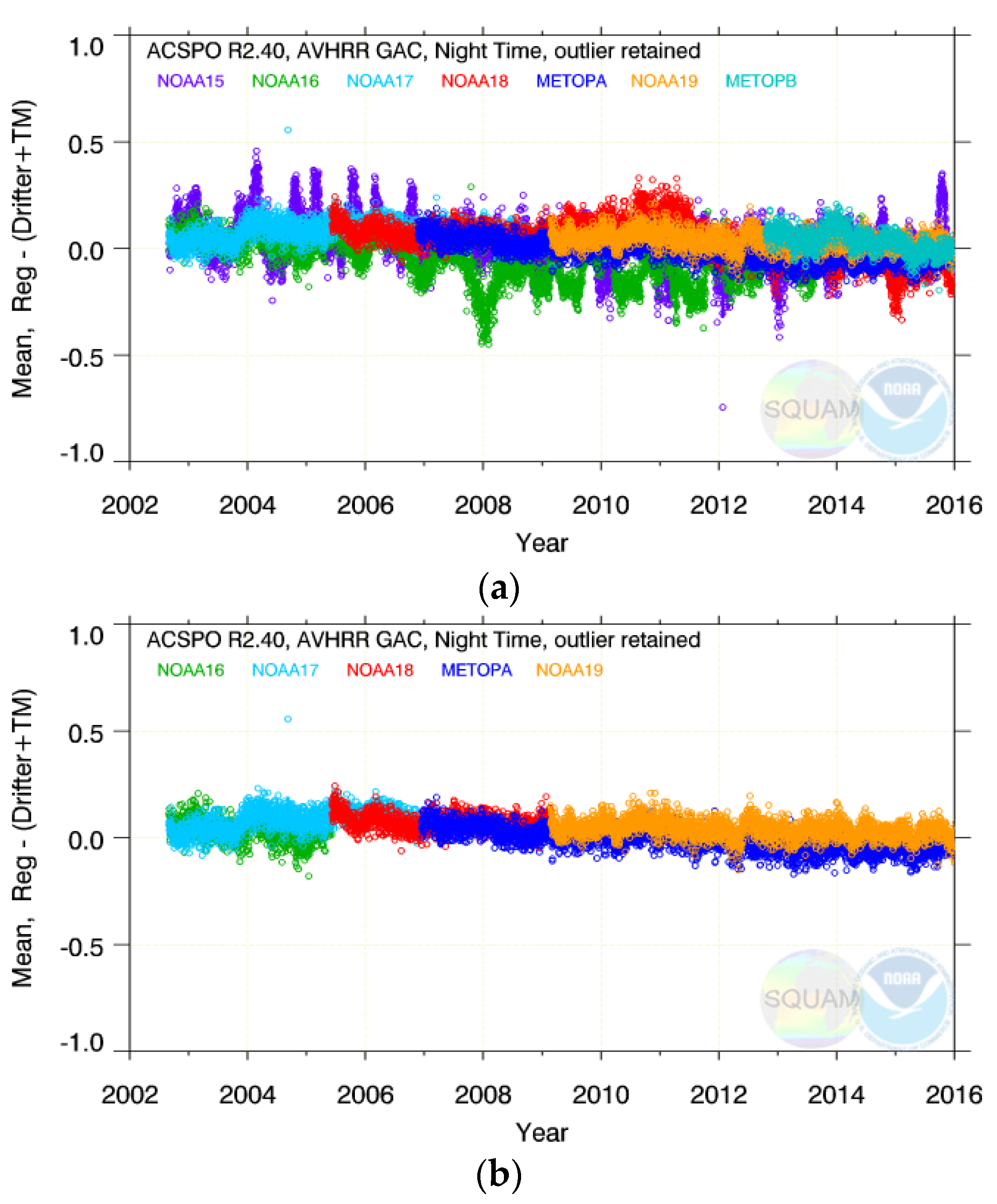
In consultation with the GPB and CRW Teams, RAN1 uses the two most stable satellites at any time, one midmorning and one afternoon. The selected satellites and periods are listed in Table 1 and the corresponding mean biases of (T_S − T_{in situ}) are shown in Figure 1b. The time series in Figure 1b have improved from Figure 1a, but some instabilities and cross-platform inconsistencies still remain.

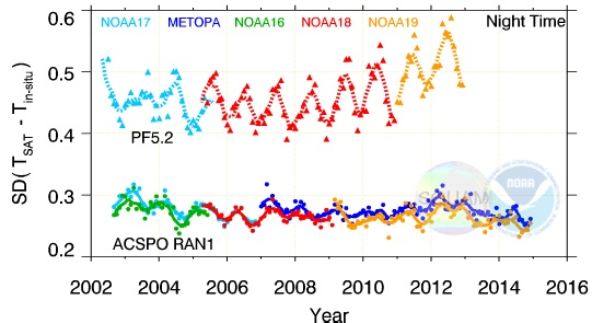
In PFV5.2, SST regression coefficients are recalculated monthly, to stabilize the retrieved SSTs in time. A similar approach was explored in RAN1, except the coefficients here are calculated daily, using a ninety-one day moving window. In RAN1, all matchups within a 91-day window are used with equal weight, whereas in PFV5.2, weighted least squares regression is employed. A moving window is used to minimize the potential month-to-month discontinuities which may be expected in the PF SSTs, and a factor of ×3 larger time window is used to reduce the uncertainty of the calculated regression coefficients while still capturing their seasonal variability.

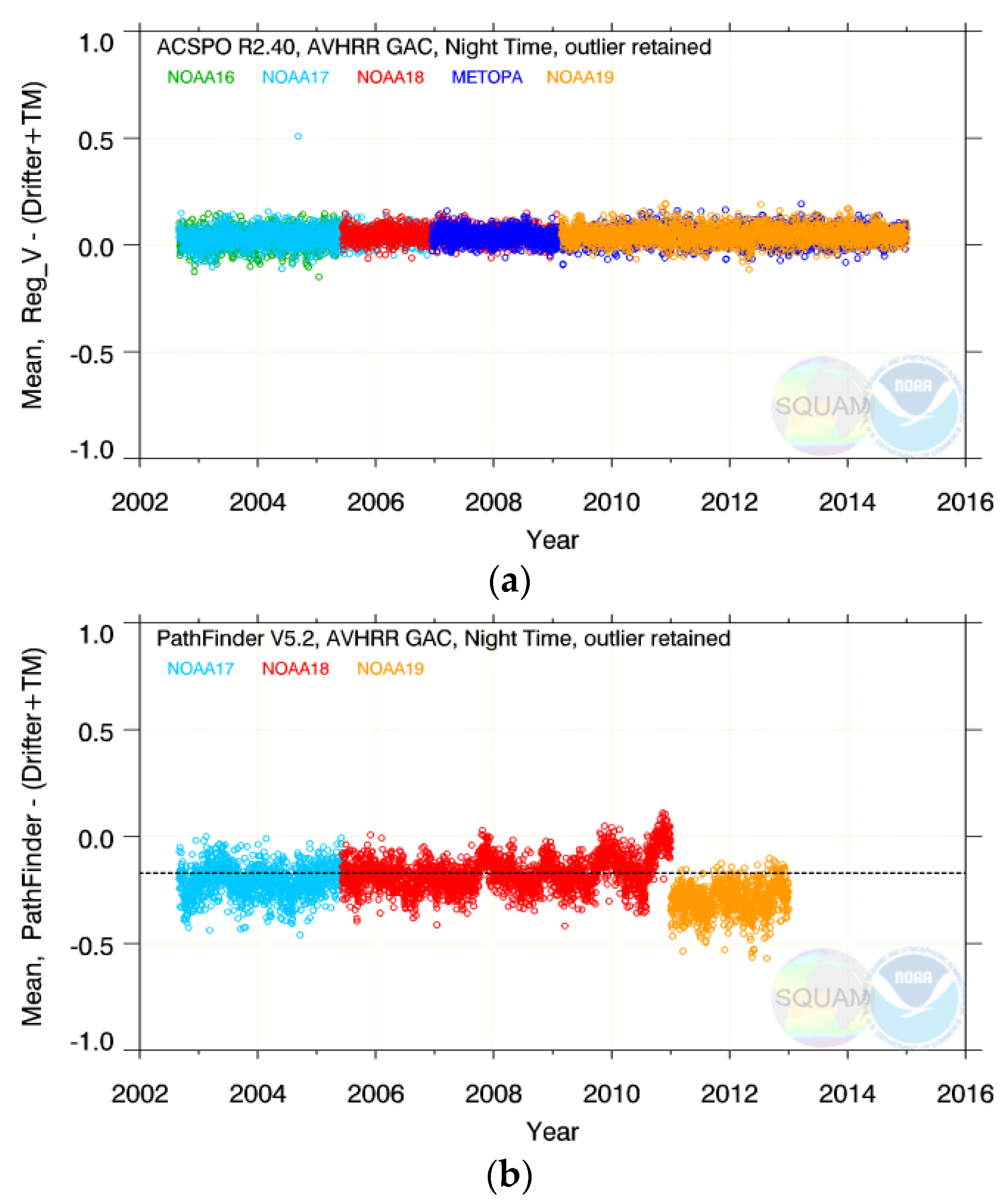
The time series of the mean biases in RAN1 and in PFV5.2 with respect to in situ data are plotted in Figure 3. Only highest quality PFV5.2 data (QL = 5) are used in this study. Analysis of one day (1 July 2010) of global NOAA-18 data has shown that the number of nighttime observations with QL = 5 was ~1.1M (M = million), compared with ~0.7M with QL = 4. The QL = 4 data are clearly degraded compared with QL = 5 (in particular, they show a ~−0.2 K colder bias, and a 0.15 K larger standard deviation, SD), and therefore they were not included in the comparisons with RAN1. Note that in PFV5.2 only one platform is processed at any time, due to the initial requirement to ensure a consistent observation time in the CDR, from only afternoon platforms (although later, midmorning NOAA-17 was used before the NOAA-18 launch). Also, PFV5.2 data are available in a delayed mode (e.g., at the time of this writing, data up to December 2012 were available, [8]).

RAN1 SSTs are more stable in time and cross-platform consistent, with typical biases of ~0 ± 0.1 K, compared with −0.17 ± 0.25 K in PFV5.2. The regression coefficients in both datasets are trained against buoys, but in PFV5.2, a −0.17 K is subtracted, to obtain the “skin” SST product [8]. Comparing Figure 3 with Figure 1b shows that using variable coefficients in RAN1 makes the SST biases smaller and more stable. In PFV5.2, the SST biases are generally grouped around the expected −0.17 K level, but are less stable in time and less cross-platform consistent. In particular, increasing positive bias is seen in the last year(s) of NOAA-18 (which according to Figure 1 and Figure 2, started showing degraded BTs and SSTs in 2010, and therefore was replaced in RAN1 by NOAA-19 in early 2009). NOAA-19 is out of family, likely due to a coding error in PFV5.2, which has degraded its cloud mask [8].

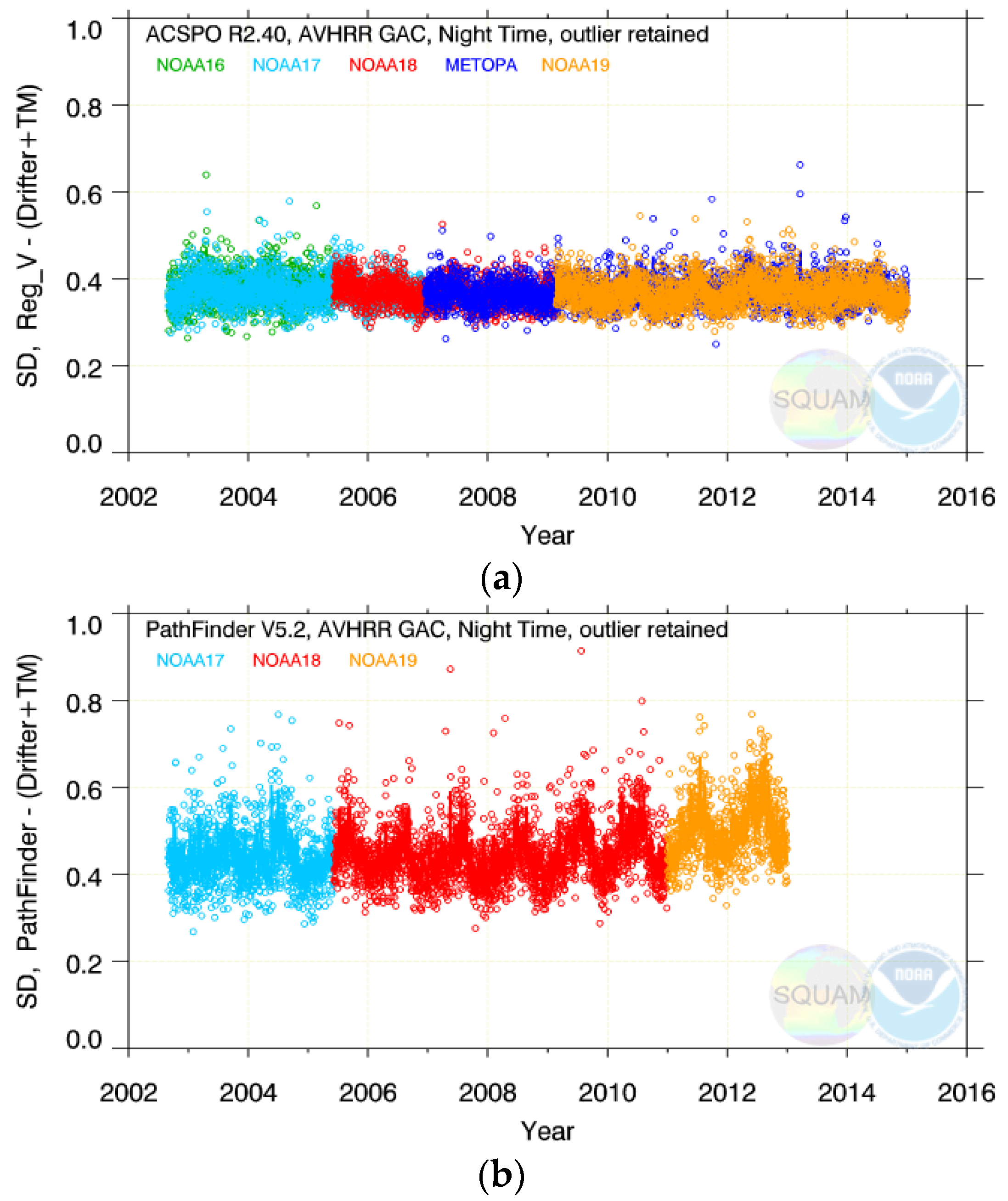
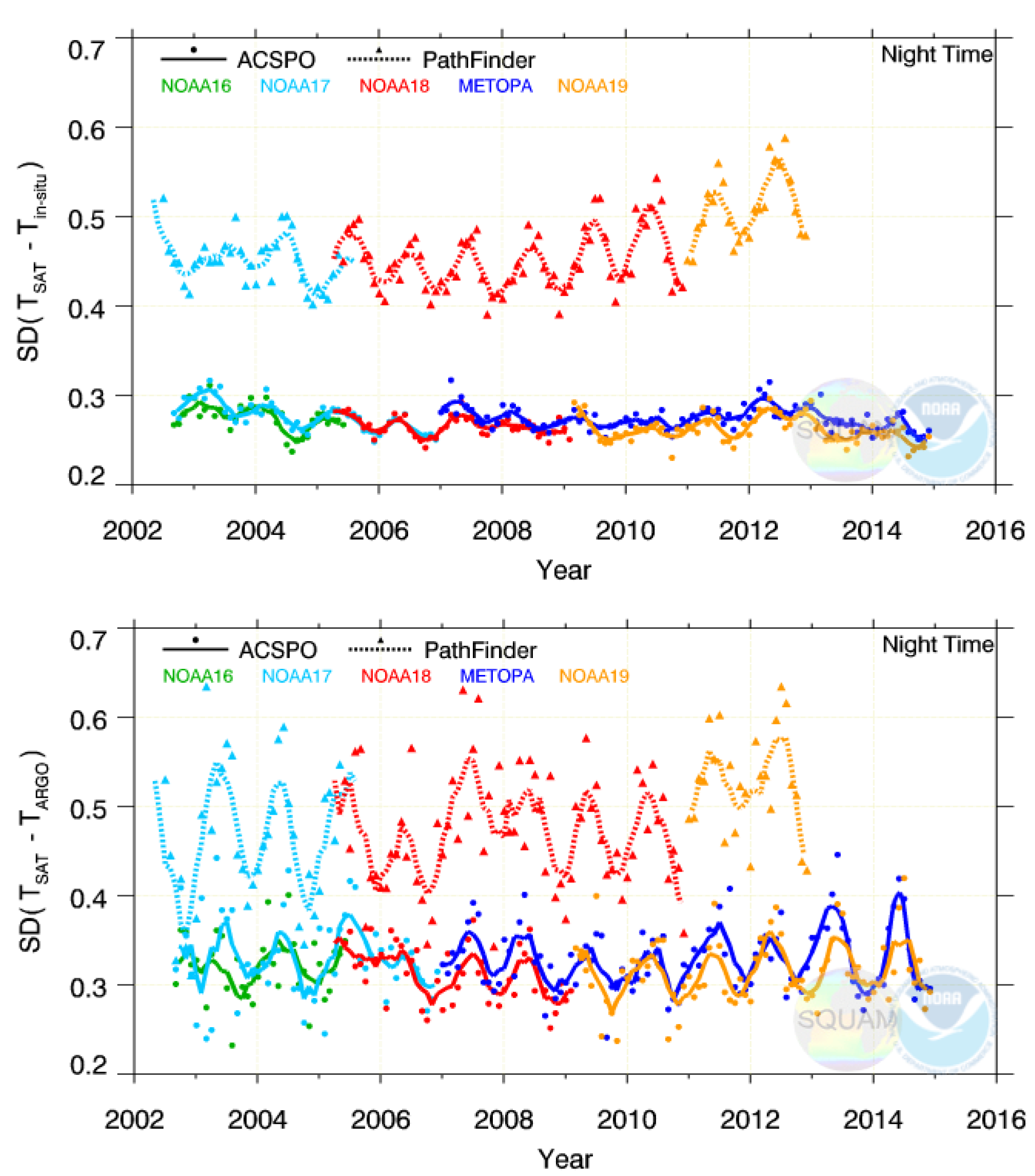
The stabilized RAN1 SDs are shown in Figure 4a. (Note that additional analyses have shown that the SDs are only minimally impacted by using variable coefficients). They are stable in time and uniform across different platforms (including between the midmorning, with a nominal equator crossing time, ECT~9:30–10 p.m., and afternoon, with a nominal ECT~2 a.m.), and typically range from 0.30 to 0.45 K, compared with 0.30–0.70 K in PFV5.2. The improved SSTs in RAN1 over PFV5.2 are largely due to the use of the ACSPO clear-sky mask [1] and SST regression algorithms [3,4]. In particular, at night, ACSPO uses the MCSST in conjunction with the transparent 3.7 µm band (see Equation (1)), whereas PFV5.2 uses the split-window NLSST with the 11/12 µm bands [8]. The ACSPO and PFV5.2 SST equations are also different. While the ACSPO equations primarily target the effect of variable VZA, the PFV5.2 algorithms are stratified by “wet” and “dry” atmospheric conditions, to mainly correct for the effect of variable water vapor in the atmosphere (see discussion in [3,4] and in Section 2.7 below). The NOAA-19 SDs are degraded, likely due to the same coding error in the corresponding PFV5.2 cloud mask mentioned earlier [8]. Overall, the conventional daily validation statistics for PFV5.2 shown in Figure 3 and Figure 4 are largely consistent with their annual robust counterparts reported in [8].

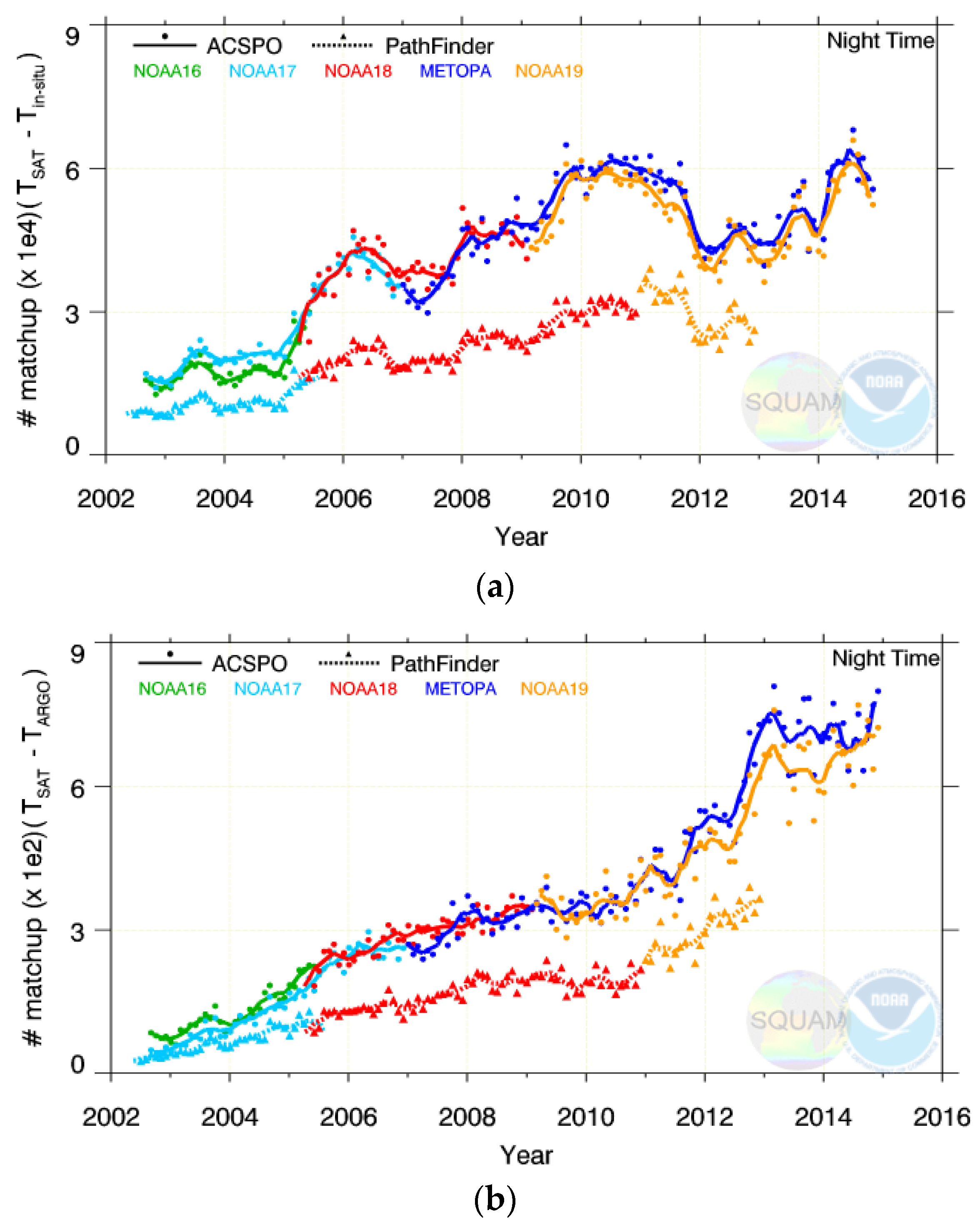
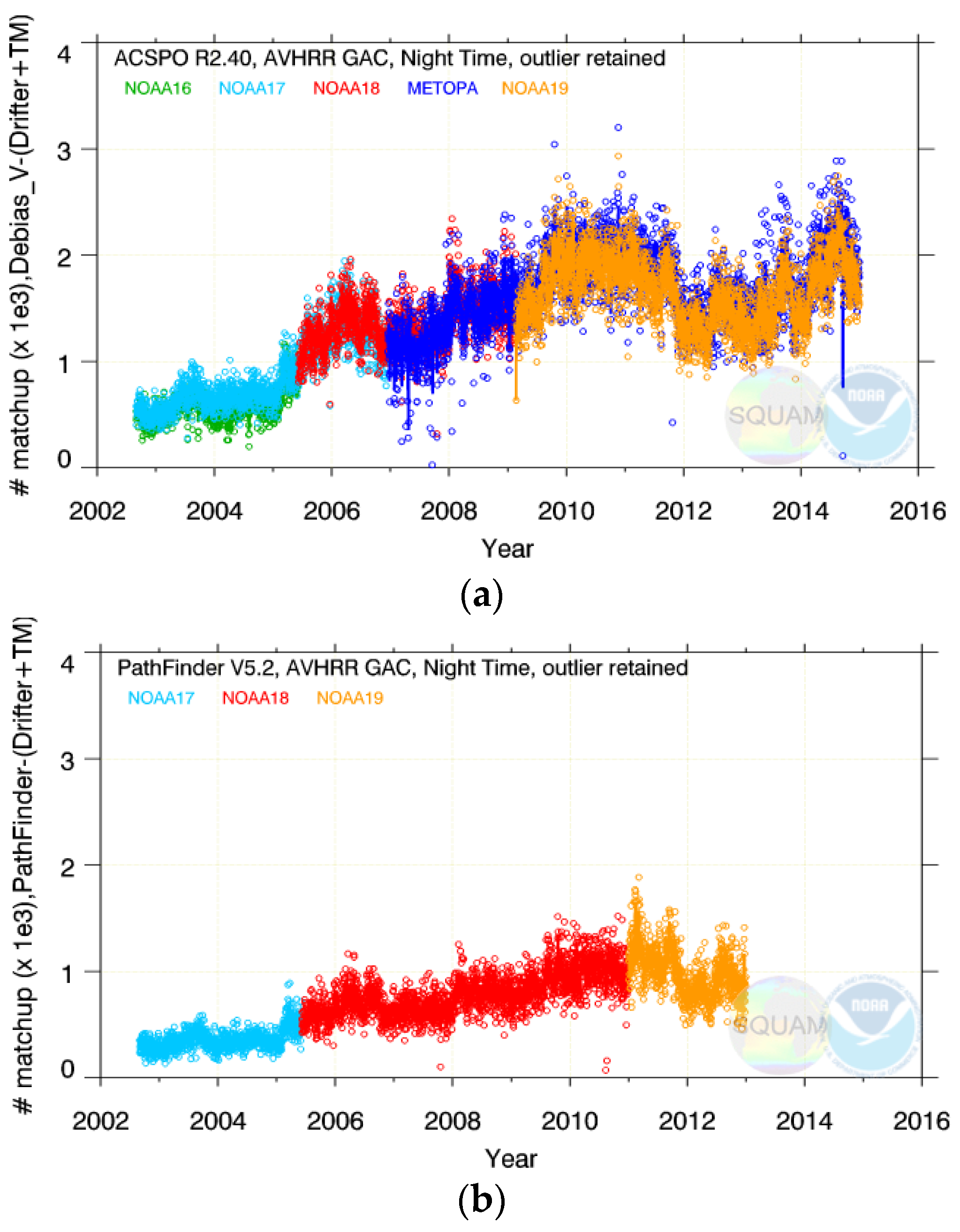
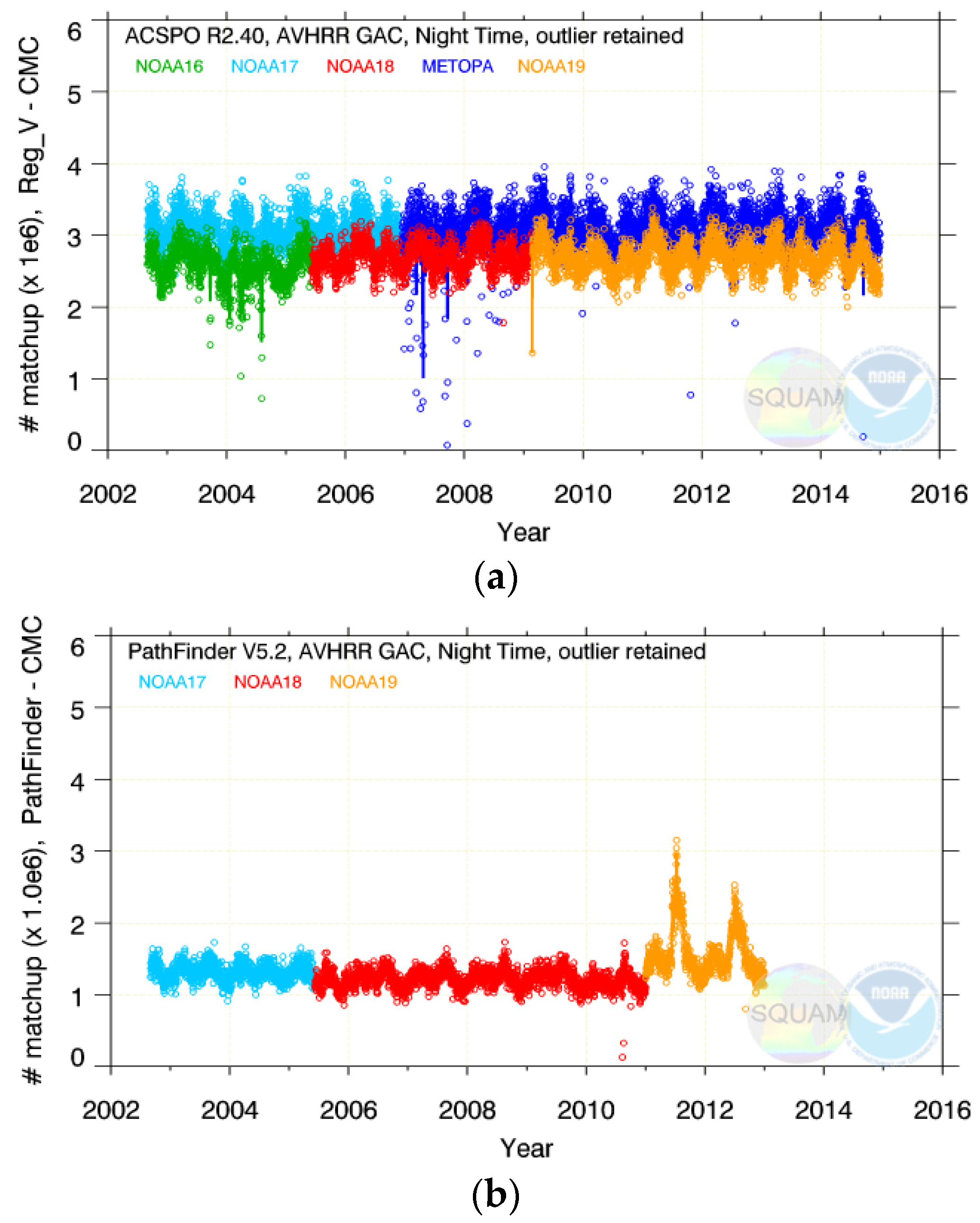
The corresponding number of matchups used to calculate the daily validation statistics in Figure 3 and Figure 4 is shown in Figure 5. It follows the evolution of the in situ fleet with time, scaled with the number of QL = 5 retrievals in RAN1 and PFV5.2. In RAN1, the number of matchups ranges from <500 in the early 2000s to >2000 in recent years. In PFV5.2, it is approximately half of RAN1 numbers. The different number of matchups in the RAN1 and PFV5.2 is due to the different number of the corresponding clear sky SST pixels with QL = 5 (shown in Figure 6). There is a clear seasonal pattern in both products, due to the alternating land-sea fraction in the Northern and Southern hemispheres following the Sun illumination periodicity. Note that direct comparison between Figure 5a,b is not straightforward, because the PFV5.2 is a remapped equal-grid 0.04° L3 product, whereas the RAN1 is an L2 product reported in the native GAC swath projection, with a ~4 km resolution at nadir and up to ~30 km at swath edge. Also, the retrievals in the PFV5.2 are only made at VZA < 55°, in contrast with the ACSPO product which covers the full swath up to VZA ~68°.

Generating a RAN1 L3 product similar to the PFV5.2 was also considered but not implemented, mainly because the mapping of the full-swath ACSPO data to a 0.04° grid would have resulted in multiple duplicates at the swath edge (where a ~30 km pixel may be mapped into multiple 0.04° grids). Using a coarser L3 grid (e.g., ~0.1°) would minimize the duplicates at swath edges (although not eliminate them completely), but at the expense of degraded spatial resolution at nadir. More discussions between the data producers and users are needed before a gridded version of RAN1 SST product can be generated.

The number of high-quality (QL = 5) nighttime SST retrievals is from ~2 to 3.5 M (M = million) GAC pixels in RAN1 whereas in PFV5.2, it is typically from 1 to 1.5 M (this latter number should be scaled by ~1.6, to account for the degraded retrievals with QL = 4). Note that the RAN1 product is available from two platforms, which effectively increases the coverage of the global ocean.

2.5. Improved RAN1 SST Using the Sensor-Specific Errors Statistics (SSES)

The international Group for High Resolution SST (GHRSST) recommends that estimates of SST bias and SD (comprising the Sensor-Specific Errors Statistics, or SSES) should be appended to each reported SST value. As of today, there is no community consensus on how the SSES should be calculated. In RAN1, the new formulation recently adopted in ACSPO is used [15]. Effectively, correcting for the SSES biases in ACSPO minimizes regional biases between the satellite “sub-skin” and in situ “bulk” SSTs, and thus results in a product which is better harmonized with the in situ SSTs measured by drifting and moored buoys.

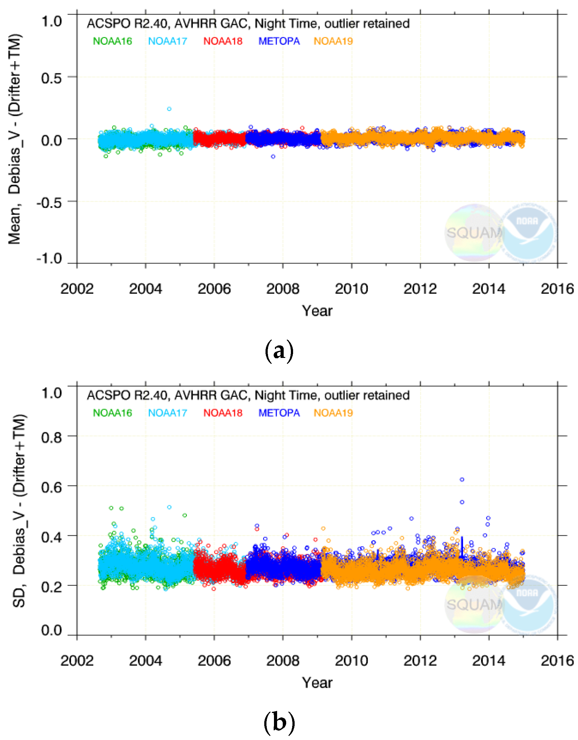
Figure 7 re-plots the time series of the SST biases and SDs from Figure 3a and Figure 4a, respectively, but after the SSES bias correction has been applied. This results in reduced SST biases with respect to in situ data (~±0.05 K vs. ±0.10 K in Figure 3a), smaller SDs (0.20–0.35 K vs. 0.30–0.45 K in Figure 4a), and overall improved stability and cross platform consistency of RAN1 SST. Therefore we recommend that in any data assimilation applications of RAN1 data, especially those blending together satellite and in situ data, and targeting “bulk” SST L4 products (such as the “foundation”, e.g., CMC SST) the SSES bias correction be applied. Also, the RAN1 data may be assimilated in analyses with weights depending on the SSES SDs (e.g., inversely proportional to their squares, see e.g., [16] and references therein).

2.6. Validation against Independent in Situ SSTs from ARGO Floats

Validation in Section 2.4 and Section 2.5 was performed against the same drifters and tropical moorings used to train the regression coefficients in RAN1. One anonymous reviewer of this paper expressed a concern that this “dependent” validation may potentially favor the RAN1 over the PFV5.2 due to over-fitting. (Recall that the PFV5.2 SST was also trained against drifting buoys, but the reviewer is correct that those were obtained from other sources than iQuam, and processed with different quality control and matchup criteria, thus making the PFV5.2 matchup data used here more “independent”.) To address this concern, additional validation was performed against ARGO floats obtained from iQuam version 2 [17], and reported in this section. In contrast with the daily validation in Section 2.4 and Section 2.5, this section reports monthly statistics, due to significantly smaller number of ARGO matchups.

Figure 8 shows the monthly number of RAN1 and PFV5.2 matchups with drifters/tropical moorings and with ARGO floats. As seen before in Figure 5, the number of matchups is up to a factor of 2 larger in RAN1 than in PFV5.2 (in proportion to the number of SST reports in the two products shown in Figure 6). Since the ARGO projects’ inception in 1999, the number of floats has been steadily increasing, resulting in <20 monthly matchups in RAN1 in 2002 and reaching >800 in late 2015. Recall that ARGO floats may only take 2–3 SST measurements a month, due to their 10-day profiling cycle, compared to continuous measurements by drifters and tropical moorings. The number of monthly matchups with ARGO floats is from two (in 2015) to three (in 2002) orders of magnitude smaller than with drifters/tropical moorings. As a result, all corresponding ARGO statistics shown in Figure 9 and Figure 10 are noisier than their drifters/tropical moorings counterparts.

Figure 9 plots mean ΔT_S’s. With respect to drifters/tropical moorings, the mean biases are ~0 ± 0.03 K in RAN1 and ~−0.17 ± 0.15 K in PFV5.2. With respect to ARGO floats, the statistics are noisier for both datasets and typically are within ~0 ± 0.1 K for RAN1 and ~−0.17 ± 0.2 K for PFV5.2. The overall observation from Figure 9 is that, with proper consideration of noise in different matchup datasets, the independent (monthly) validation against ARGO floats is in good qualitative, and even quantitative, agreement with the dependent (daily and monthly) validation against drifters/tropical moorings.

Figure 10 plots SDs of the ΔT_S’s. A seasonal signal is seen in both datasets (more so in PFV5.2). Typical monthly SDs with respect to drifters and tropical moorings are 0.28 ± 0.05 K in RAN1 and 0.47 ± 0.10 K in PFV5.2. With respect to ARGO floats, the corresponding monthly SDs are 0.32 ± 0.08 K in RAN1 and 0.50 ± 0.15 K in PFV5.2.

Overall, analyses in this section show that independent validation against ARGO floats, although noisier due to much smaller matchup samples, is qualitatively consistent with the results obtained against the dependent dataset of drifters/tropical moorings. The RAN1 mean biases and SDs are generally smaller and more stable in time, and show better cross-platform consistency, against both types of in situ data. The evaluation of VZA and regional performance of satellite SST in the next section was therefore performed against more abundant drifters/tropical moorings, to minimize the noise in the matchup dataset and to facilitate quantifying possible SST residuals and artifacts.

2.7. Performance of RAN1 SST as a Function of Latitude and VZA

Mean biases and SDs are convenient metrics to measure the global performance of various SST products and to compare different products. For users, however, it is also important to ensure that the performance is maximally uniform across the full retrieval domain.

The accuracy of satellite SSTs depends upon many factors, one of the most important being the atmosphere between the satellite sensor and ocean pixel. In the SST bands, the atmospheric attenuation and re-emission mainly depends on the total precipitable water, TPW, and VZA. One might expect that the two would aggregate as TPW × sec(VZA). However, in reality they are not fully coupled (due to e.g., decreasing surface emissivity and increasing cloud across the swath). All current atmospheric correction algorithms fall under two broad categories of “MCSST” and “NLSST”, but the actual equations used in different retrieval groups differ. Some (e.g., employed in OSI SAF) explicitly target the VZA dependencies, whereas others focus on the TPW correction (e.g., the algorithm employed in PFV5.2). Based on systematic comparisons in [3,4], the OSI SAF type MCSST/NLSST algorithms (represented by Equations (1) and (2) above) were found to be more efficient and therefore adopted in ACSPO [3]. Proper handling of the VZA dependencies is critically important in ACSPO, which was the first SST system to attempt high-quality retrievals in the full sensor swath (up to VZA~68°; cf. VZA~55° cut-off in PFV5.2). The reality however is more complex than a simplistic “TPW-VZA” model, and there are other factors involved in the retrievals. Assuming that those may be aggregated and approximated as a function of latitude, the future release of PF plans to explore a new implementation of the SST regression algorithm, LATBAND [8] (which targets minimizing SST errors as a function of latitude; note that the LATBAND algorithm was also analyzed in [3]). In this section, the performance of the satellite SSTs is therefore evaluated as a function of VZA (only in RAN1, because the VZA is not reported in PFV5.2 data files) and latitude (in both RAN1 and PFV5.2).

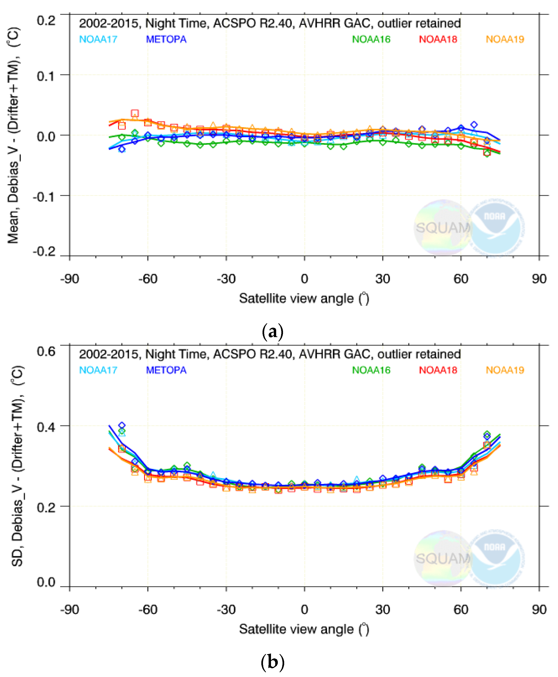
Figure 11 plots mean biases and SDs in RAN1 SST as a function of VZA, by platform. The biases are close to zero, within several hundredths of a degree Kelvin, and near-flat across the full swath. Note a slight trend across the swath (positive for all PM platforms, which descend at night and negative for all AM platforms, which ascend), due to the satellite sensor looking at systematically different parts of the SST diurnal cycle across the swath. The SDs are also highly consistent across platforms, but non-uniform across the swath, increasing from ~0.25 K at nadir to ~0.40 K toward the edge. This degradation is expected, due to reduced atmospheric transmission and surface emission, and increased atmospheric reemission, which together lead to a progressively smaller surface signal at slant angles. The actual degradation may appear small and disproportionate to, e.g., a factor of ×3 thicker atmosphere at VZA ~68°. However, one should keep in mind that the validation SD represents a combination of the atmospheric correction and other errors (such as e.g., uncertainty in the in situ data and matchup errors). Accounting for these “pedestal” contributions, which are uniform across the swath, will increase the contrast between the nadir and swath edge SDs.

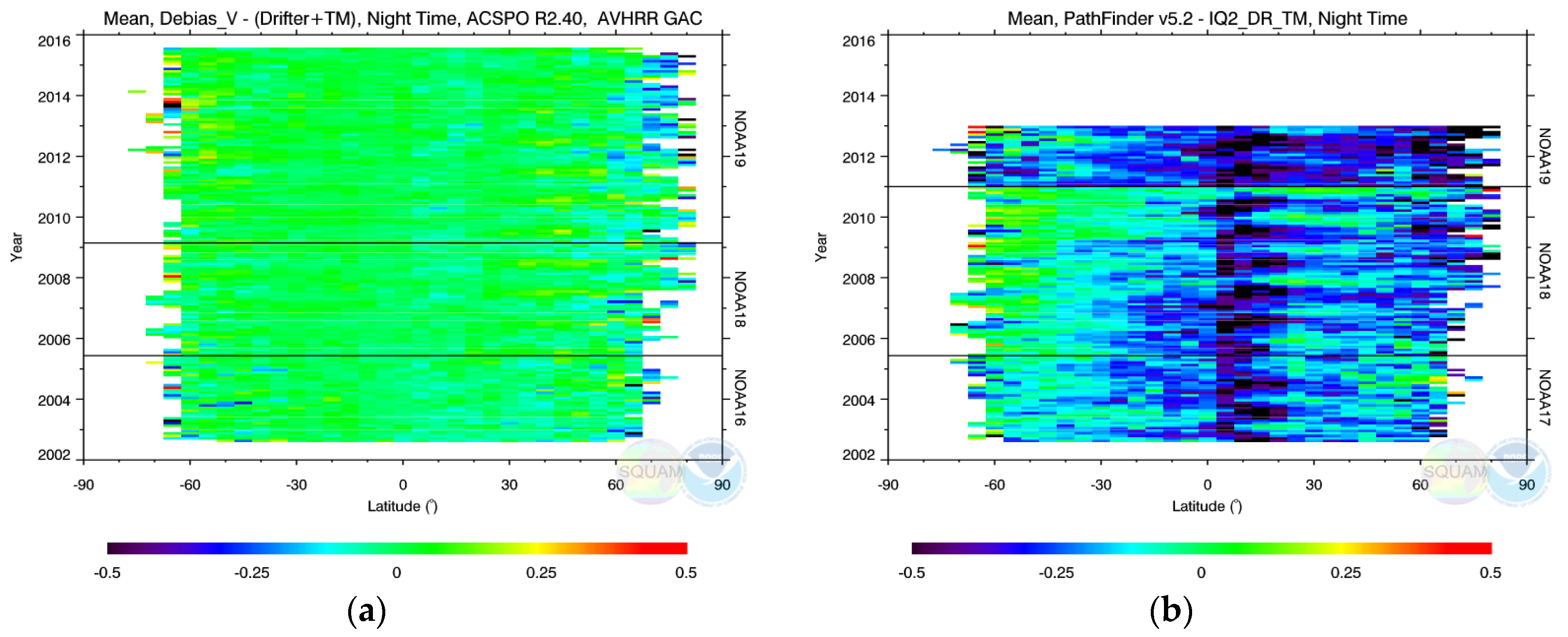
Turning to geographical biases, Figure 12 shows Hovmöller diagrams of the mean SST biases. The RAN1 biases are relatively flat in the full domain. A few larger and intermittent (positive/negative) anomalies are seen only in high latitudes, which are least populated with in situ data. Note that in the early 2000s, the number of drifters in the Arctic above 70° N was very limited, and increased after ~2008. In the Antarctic, very few observations are still found below 70° S, even at the present time. Figure 12b shows that the PFV5.2 biases (which recall are expected to be centered at −0.17 K) are highly non-uniform in space and time. In particular, there are sharp discontinuities between NOAA-18 and −19 (consistent with the time series in Figure 3b and Figure 9b; likely due to the coding bug for NOAA-19 in PFV5.2 as mentioned earlier), and between the Northern and Southern hemispheres.

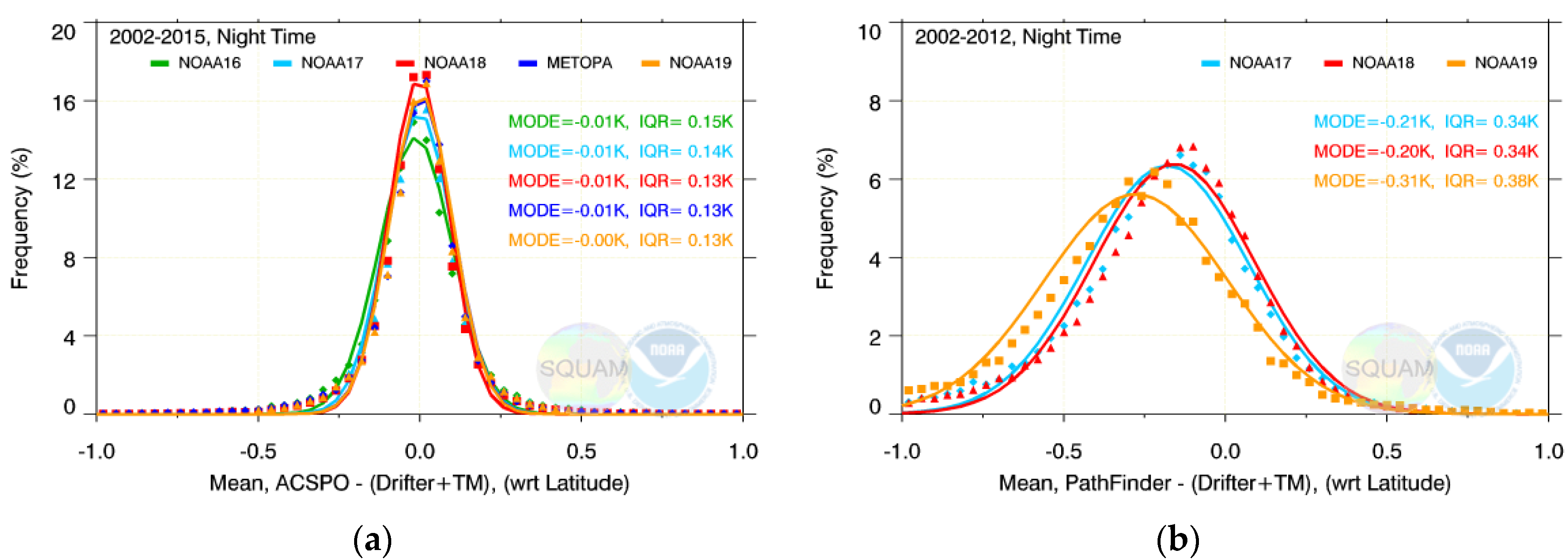
To estimate the magnitude of spatial and temporal non-uniformities in Figure 12 quantitatively, Figure 13 plots their corresponding histograms. In RAN1, the biases are near-Gaussian, centered at ~0 K and consistent between all five platforms. The inter-quartile ranges, IQR (defined as Q3-Q1) are ~0.14 K, meaning that 50% of regional biases are within ±0.07 K (Figure 13a further shows that the vast majority of RAN1 biases fall within ±0.3 K). In PFV5.2, the mean biases are centered close to the expected −0.17 K for NOAA-17 and -18 but are ~−0.1 K colder for NOAA-19, and less symmetric. The IQR~0.36 K suggests that 50% of regional biases in PFV5.2 fall within ±0.18 K, with a measurable fraction of cold biases (suggesting residual cloud) extending to <−1 K and warm biases to ~+0.5 K.

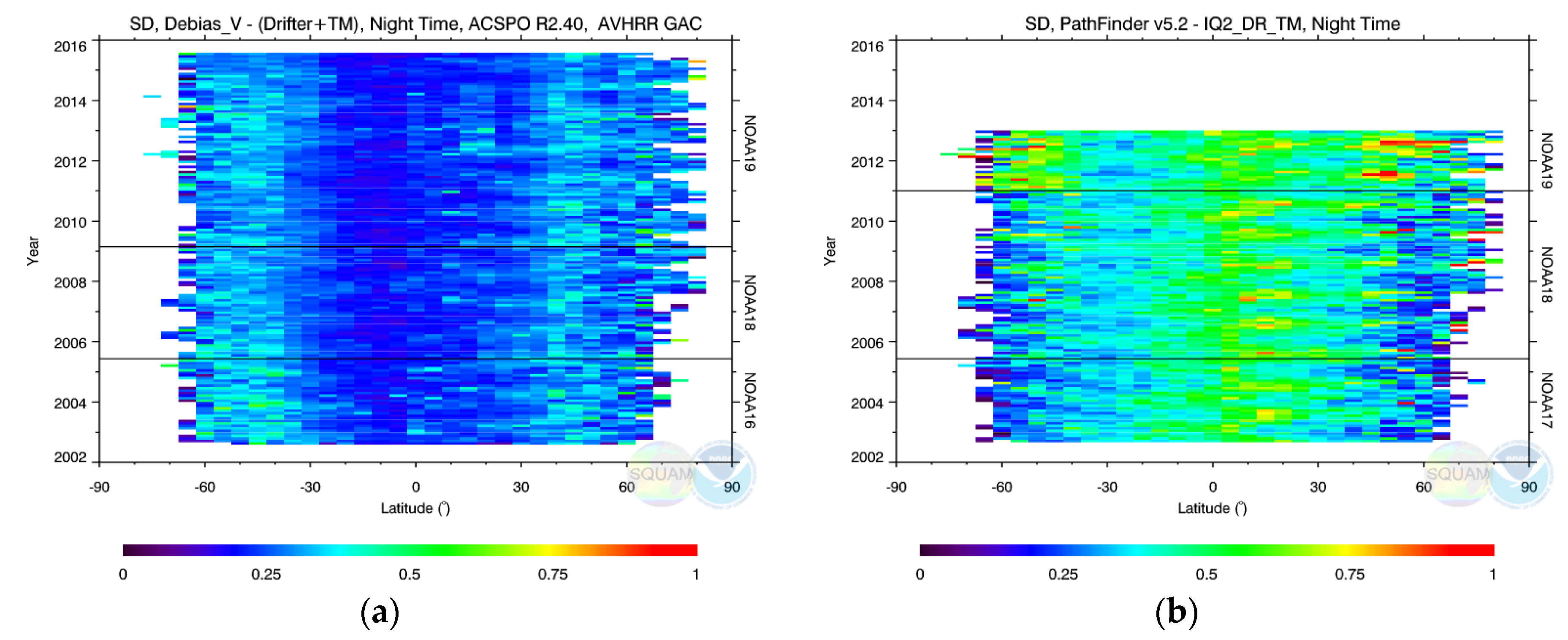
Figure 14 further shows the spatiotemporal structure of the corresponding SDs. The RAN1 SDs are more uniform in space and time, typically ranging from 0.25 K to 0.5 K. In contrast, the PFV5.2 SDs are larger in magnitude (typically from 0.4 to 0.7 K), and more variable in space and time. Note that different spatiotemporal patterns in the SDs between RAN1 and PFV5.2 are at least in part due to the different SST algorithms used in the two products. In particular, the PFV5.2 split-window (11/12 µm) NLSST algorithm is more sensitive to the increased TPW in the tropics, compared with the RAN1 dual-window (3.7/11/12 µm) MCSST algorithm.

Analyses in this section show that compared to PFV5.2, the RAN1 SST performance is consistently superior and more uniform across different satellites and in the full retrieval domain (in particular, as a function of VZA and latitude).

3. Summary and Future Work

Until lately, the NOAA/NASA Pathfinder Ocean dataset remained the only available long-term global AVHRR SST record. It has been used in many studies and proved to be instrumental in a number of analyses and applications, including creating several long-term L4 SST analyses (e.g., [18,19]). In recent years, in response to the evolving needs of the user community, alternative long-term AVHRR L2/3 SST records have emerged, including the Climate Change Initiative (CCI) AVHRR L2 dataset from 1991 to 2010 [20] and the RAN1 dataset from 2002-pr [this study]. In the same way that different L4 analyses, produced from the same input satellite L2/L3 and in situ SST data, while using different analysis schemes and targeting different user applications can exhibit different performance, (e.g., [21] and references therein), different satellite L2/3 SST products with varying performance may be likewise derived from the same sensor counts reported in the L1b files, but using different calibration, sampling, cloud screening and SST retrieval algorithms. Analyses in SQUAM clearly show that SST products produced by different providers, with different processing algorithms, may differ significantly, even when the same input data are used [11].

Comparisons with the PFV5.2 performed in this study suggest that RAN1 provides more complete coverage of the global ocean, due to using the full sensor swath (VZA up to 68°) and two satellites at a time (one midmorning and one afternoon), compared to the VZA = 55° cut-off and one satellite at a time in PFV5.2. The ACSPO clear-sky mask is somewhat more liberal, which however does not result in degraded validation statistics. On the contrary, all RAN1 validation time series appear more stable in time, uniform across the full retrieval space, and cross-platform consistent. Note that the ultimate evaluation of the RAN1 SST, and its relative merits compared with the PFV5.2 and CCI, lies with the users. In addition to the NOAA GPB/CRW teams, the U. Maryland ocean assimilation group [22] expressed interest in evaluating the RAN1 product, mainly due to its availability beyond 2012 where the PFV5.2 has stopped. Evaluations by the UMD and GPB/CRW teams are currently underway and the results will be reported elsewhere.

Also, the AVHRR and (A)ATSR CCI SSTs are being added to SQUAM so that in the near future, users can easily compare the retrieval domains and performance statistics of the various reprocessed datasets, and select data appropriate for their applications. In particular, deriving SST regression coefficients from RTM and moving away from buoy matchups was explored in the CCI. Our experience with RAN1 and AVHRR L1b analyses in [14] suggest that the current instabilities in the AVHRR sensor calibration should be minimized first, before the advantages of physical SST retrievals can be fully realized. Future inter-comparisons of RAN1 and CCI products will help to quantify the real versus expected improvements due to the use of more physically based retrievals with the current AVHRR L1b data.

The RAN1 product is experimentally produced at STAR in the GHRSST Data Specification version 2 (GDS2) format with a ~1 month latency (in contrast to the PFV5.2 and CCI products, which as of this writing are only available through 2012 and 2010, respectively). The data product is available from the authors upon request. Work is underway with the NOAA Office of Satellite Products and Operations (OSPO) to generate the AVHRR GAC SST product in GDS2 format operationally and archive it with the NASA Physical Oceanography Distributed Active Archive Center (PO.DAAC; http://podaac.jpl.nasa.gov/) and the NOAA National Center for Environmental Information (NCEI; www.ncei.noaa.gov/). Once archival commences, the data will be available to users in real time, and the full RAN1 record starting from August 2002 will be back-filled and available for download from these official GHRSST centers. Once newer ACSPO versions emerge, the complete record will be reprocessed and archived.

Detailed analyses of the RAN1 SSTs in [4] suggest that it can be improved, by tuning the clear-sky mask and SST algorithms, to further reduce regional, seasonal, and swath biases in the regression SSTs. Pending these future improvements in RAN, the users assimilating the RAN1 SST in their analyses are encouraged to first apply the SSES bias correction, which according to our analyses strongly minimizes regional biases and improves the consistency of the retrieved SSTs with in situ data, and therefore is expected to minimize the need for empirical bias correction on the users’ side. Note that the SSES is available in the ACSPO files, but its application is left to users’ discretion.

At this time, the AVHRR sensor calibration remains the major limitation to the SST performance in RAN1. In particular, the data in Figure 2 unambiguously support the major recommendation in the NRC (2004) report on satellite climate data records (CDR) [23] which states that high quality fundamental climate data records (FCDRs; the AVHRR BTs) are a prerequisite for the high quality thematic climate data records (TCDRs; the SST). To that end, the current priority is to better understand and resolve the root causes of the unstable AVHRR calibration and generate an improved AVHRR/3 FCDR [14], at which time the need for the variable regression coefficients will be minimized and a more stable SST TCDR (ACSPO RAN) will be produced.

Work continues with the users, including the GPB/CRW and UMD Teams, to evaluate the results of RAN1 and subsequent RANs, and make improvements as needed. Following users’ requests, we are exploring extending the AVHRR RAN time series, initially back to mid-1990s (the time when first GOES data suitable for SST retrievals was introduced), and then further back in time to cover the full AVHRR era from 1981 to present. Adjustments to the current approaches may be needed as one goes back in time, when in situ data were sparser, the satellites and their overlaps fewer, and quality of AVHRR Level 1b data degraded. Also, accurate atmospheric correction during the two major volcanic eruptions—El Chichón in April 1982 and Mount Pinatubo in August 1991—will be challenging with the current MCSST/NLSST algorithms. These issues will be analyzed and addressed as they occur.

References

1. Petrenko, B.; Ignatov, A.; Kihai, Y.; Heidinger, A. Clear-sky mask for the advanced clear-sky processor for oceans. J. Atmos. Ocean. Technol. 2010, 27, 1609–1623. [Google Scholar] [CrossRef]
2. Liang, X.; Ignatov, A.; Kihai, Y. Implementation of the Community Radiative Transfer Model (CRTM) in Advanced Clear-Sky Processor for Oceans (ACSPO) and validation against nighttime AVHRR radiances. J. Geophys. Res. 2009, 114. [Google Scholar] [CrossRef]
3. Petrenko, B.; Ignatov, A.; Kihai, Y.; Stroup, J.; Dash, P. Evaluation and selection of SST regression algorithms for JPSS VIIRS. J. Geophys. Res. 2014, 119, 4580–4599. [Google Scholar] [CrossRef]
4. Petrenko, B.; Ignatov, A.; Kihai, Y.; Zhou, X.; Stroup, J. SST Algorithms in ACSPO reanalysis of AVHRR GAC data from 2002–2013. Proc. SPIE 2014. [Google Scholar] [CrossRef]
5. Liu, G.; Heron, S.; Eakin, M.; Muller-Karger, F.; Vega-Rodriguez, M.; Guild, L.; Rauenzahn, J.; Geiger, E.; Skirving, W.; Burgess, T.; et al. Reef-scale thermal stress monitoring of coral ecosystems: New 5-km global products from NOAA coral reef watch. Remote Sens. 2014, 6, 11579–11606. [Google Scholar] [CrossRef]
6. Kilpatrick, K.A.; Podestá, G.P.; Evans, R. Overview of the NOAA/NASA advanced very high resolution radiometer Pathfinder algorithm for sea surface temperature and associated matchup database. J. Geophys. Res. 2001, 106, 9179–9197. [Google Scholar] [CrossRef]
7. Casey, K.; Brandon, T.; Cornillon, P.; Evans, R. The past, present, and future of the AVHRR pathfinder SST program. In Oceanography from Space: Revisited; Barale, V., Gower, J.F.R., Alberotanza, L., Eds.; Springer: Berlin, Germany, 2010. [Google Scholar] [CrossRef]
8. Kilpatrick, K.A. Climate Algorithm Theoretical Basis Document (C-ATBD): Pathfinder SST; CDRP-ATBD-0099 v2; 2013. Available online: http://www1.ncdc.noaa.gov/pub/data/sds/cdr/CDRs/Sea_Surface_Temperature_Pathfinder/AlgorithmDescription.pdf (accessed on 23 March 2016).
9. Brasnett, B.; Surcel-Colan, D. Assimilating retrievals of sea surface temperature from VIIRS and AMSR2. J. Atmos. Ocean. Technol. 2016, 33, 361–375. [Google Scholar] [CrossRef]
10. Xu, F.; Ignatov, A. In situ SST quality monitor (iQuam). J. Atmos. Ocean. Technol. 2014, 31, 164–180. [Google Scholar] [CrossRef]
11. Dash, P.; Ignatov, A.; Yuri, K.; Sapper, J. The SST quality monitor (SQUAM). J. Atmos. Ocean. Technol. 2010, 27, 1899–1917. [Google Scholar] [CrossRef]
12. Liang, X.; Ignatov, A. Monitoring of IR clear-sky radiances over oceans for SST (MICROS). J. Atmos. Ocean. Technol. 2011, 28. [Google Scholar] [CrossRef]
13. Liang, X.; Ignatov, A. AVHRR, MODIS, and VIIRS radiometric stability and consistency in SST bands. J. Geophys. Res. 2013, 118. [Google Scholar] [CrossRef]
14. He, K.; Ignatov, A.; Kihai, Y.; Cao, C.; Stroup, J. Sensor Stability for SST (3S): Toward improved long-term characterization of AVHRR thermal bands. Remote Sens. 2016. submitted. [Google Scholar]
15. Petrenko, B.; Ignatov, A.; Kihai, Y.; Dash, P. Sensor-specific error statistics for SST in the Advanced Clear-Sky Processor for Oceans. J. Atmos. Ocean. Technol. 2016, 33, 345–359. [Google Scholar] [CrossRef]
16. Roger, C. Retrieval of atmospheric temperature and composition from remote measurements of thermal radiation. Rev. Geophys. Space Phys. 1976, 14, 609–624. [Google Scholar]
17. Ignatov, A.; Xu, F.; Zhou, X. Redesigned in situ SST quality monitor: iQuam version 2. J. Atmos. Ocean. Technol. 2016. submitted. [Google Scholar]
18. Reynolds, R.; Smith, T.; Liu, G.; Chelton, D.; Casey, K.; Schlax, M. Daily high-resolution-blended analysis for sea surface temperature. J. Clim. 2007, 20, 5473–5496. [Google Scholar] [CrossRef]
19. Roberts-Jones, J.; Fiedler, E.; Martin, M. Daily, global, high-resolution SST and sea ice reanalysis for 1985–2007 using the OSTIA system. J. Clim. 2012, 9, 6215–6232. [Google Scholar] [CrossRef]
20. Merchant, C.; Embury, O.; Roberts-Jones, J.; Fiedler, E.; Bulgin, C.; Corlett, G.; Good, S.; McLauren, A.; Rayner, N.; Morak-Bozzo, S.; et al. Sea surface temperature datasets for climate applications from phase 1 of the European Space Agency Climate Change Initiative (SST CCI). Geosci. Data J. 2014, 1, 179–191. [Google Scholar] [CrossRef]
21. Dash, P.; Ignatov, A.; Martin, M.; Donlon, C.; Brasnett, B.; Reynolds, R.W.; Banzon, V.; Beggs, H.; Cayula, J.F.; Chao, Y.; et al. Group for high resolution sea surface temperature (GHRSST) analysis fields inter-comparisons. Part 2: Near real time web-based Level 4 SST quality monitor (L4-SQUAM). Deep Sea Res. II Top. Stud. Oceanogr. 2012, 77, 31–43. [Google Scholar] [CrossRef]
22. Chepurin, G.; Carton, J. Subarctic and Arctic sea surface temperature and its relation to ocean heat content 1982–2010. J. Geophys. Res. 2012, 117. [Google Scholar] [CrossRef]
23. National Research Council (NRC). Climate Data Records from Environmental Satellites; Interim Report; The National Academies Press: Washington, DC, USA, 2004; Available online: http://www.nap.edu/catalog/10944/climate-data-records-from-environmental-satellites-interim-report (accessed on 23 March 2016).
Figure 1. Mean nighttime ΔTS = TSTin situ for TS derived using static regression coefficients: (a) all data; (b) used in RAN1. Each data point represents a daily statistic based on matchups with in situ SSTs (from 500 to 2000; cf. discussion in Section 2.4).
Remotesensing 08 00315 g001
Figure 2. Mean nighttime (a) ΔTS = TSTL4 and (b) ΔTB = TOTM (in band 3b) corresponding to Figure 1a. Each data point represents a daily statistic based on matchups with CMC L4 SST (from 2.0 to 3.5 M; M = million).
Remotesensing 08 00315 g002
Figure 3. Mean nighttime biases ΔTS = TSTin situ in: (a) RAN1; (b) Pathfinder version 5.2 (PFV5.2) for the time period covered by RAN1. (The PFV5.2 reports “skin” SST, obtained by subtracting −0.17 K from the “bulk” SST tuned to buys. The expected −0.17 K bias is shown with the dotted line).
Remotesensing 08 00315 g003
Figure 4. Standard deviations (SD) of ΔTS = TSTin situ in: (a) RAN1; (b) PFV5.2.
Remotesensing 08 00315 g004
Figure 5. Number of daily matchups with in situ data used in producing Figure 3 and Figure 4: (a) RAN1; (b) PFV5.2.
Remotesensing 08 00315 g005
Figure 6. Daily number of nighttime SSTs with QL = 5 in: (a) RAN1; (b) PFV5.2.
Remotesensing 08 00315 g006
Figure 7. (a) Biases and (b) SDs of RAN1 SST re-plotted from Figure 3a and Figure 4a but after applying the Sensor-Specific Errors Statistics (SSES) bias correction.
Remotesensing 08 00315 g007
Figure 8. Monthly number of nighttime matchups with: (a) drifters/tropical moorings; (b) ARGO floats. These matchups were used for producing Figure 9 and Figure 10 below.
Remotesensing 08 00315 g008
Figure 9. Monthly mean nighttime biases of ΔTS = TSTin situ against (a) drifters/tropical moorings; and (b) ARGO floats. (RAN1 SSTs are SSES bias corrected.)
Remotesensing 08 00315 g009
Figure 10. Same as in Figure 9 but for the SDs of ΔTS = TSTin situ.
Remotesensing 08 00315 g010
Figure 11. View zenith angle (VZA) dependencies of (a) mean biases and (b) SDs of ΔTS = TSTin situ in RAN1 from all matchups aggregated by platform.
Remotesensing 08 00315 g011
Figure 12. Hovmöller diagrams of mean (over 5° × month space-time boxes) biases ΔTS = TSTin situ: (a) RAN1 (b) PFV5.2.
Remotesensing 08 00315 g012
Figure 13. Histograms produced from the corresponding Hovmöller plots in Figure 12: (a) RAN1; (b) PFV5.2. IQR = Inter-Quartile Range (defined as Q3-Q1).
Remotesensing 08 00315 g013
Figure 14. Same as in Figure 12 but for the corresponding SDs: (a) RAN1; (b) PFV5.2.
Remotesensing 08 00315 g014