Article

An Online System for Nowcasting Satellite Derived Temperatures for Urban Areas

by
Iphigenia Keramitsoglou
1,†,
Chris T. Kiranoudis
1,2,†,
Panagiotis Sismanidis
1,2,*,† and
Klemen Zakšek
1,3,†
1
Institute for Astronomy, Astrophysics, Space Applications and Remote Sensing, National Observatory of Athens, Athens GR-15236, Greece
2
School of Chemical Engineering, National Technical University of Athens, Athens GR-15780, Greece
3
Institute of Geophysics, Center for Earth System Research and Sustainability, University of Hamburg, Hamburg DE-20146, Germany
*
Author to whom correspondence should be addressed.
These authors contributed equally to this work.
Remote Sens. 2016, 8(4), 306; https://doi.org/10.3390/rs8040306
Submission received: 11 February 2016 / Revised: 24 March 2016 / Accepted: 31 March 2016 / Published: 6 April 2016

Abstract

:
The Urban Heat Island (UHI) is an adverse environmental effect of urbanization that increases the energy demand of cities and impacts human health. The study of this effect for monitoring and mitigation purposes is crucial, but it is hampered by the lack of high spatiotemporal temperature data. This article presents the work undertaken for the implementation of an operational real-time module for monitoring 2 m air temperature (TA) at a spatial resolution of 1 km based on the Meteosat Second Generation—Spinning Enhanced Visible and Infrared Imager (MSG-SEVIRI). This new module has been developed in the context of an operational system for monitoring the urban thermal environment. The initial evaluation of TA products against meteorological in situ data from 15 cities in Europe and North Africa yields that its accuracy in terms of Root Mean Square Error (RMSE) is 2.3 °C and Pearson’s correlation coefficient (Rho) is 0.95. The temperature information made available at and around cities can facilitate the assessment of the UHIs in real time but also the timely generation of relevant higher value products and services for energy demand and human health studies. The service is available at http://snf-652558.vm.okeanos.grnet.gr/treasure/portal/info.html.

Graphical Abstract

1. Introduction

The rapid urbanization process that took place the last decades has been marked by profound environmental, economic, and social impacts [1,2]. One of the most adverse environmental effects is the urban heat island (UHI) [3]. This effect refers to the relative warmth of the urban areas with respect to their surrounding rural areas and results primarily from the conversion of natural lands to impervious surfaces (e.g., asphalt, buildings, etc.). Specifically, the latter have considerably different thermodynamic characteristics (e.g., higher thermal conductivity and specific heat capacity) with respect to the former and, thus, change the local heat balance of urban areas. This heat balance change affects the local weather and climate and, in combination with a series of other adverse environmental effects (i.e., the decrease in evapotranspiration; the anthropogenic heat fluxes; the reduction in turbulent heat transport; and air pollution), cause the UHI effect [3]. Although many UHI mitigation strategies have been proposed lately [4,5,6], UHIs still occur in almost all urban areas—independently of city size and climate zone—and their study, as well as the assessment of their impact, is of great importance. This is because the UHI effect has been associated with a range of issues, such as increased energy demand and human health problems (such as thermal discomfort and increased mortality during heatwaves) [7,8,9,10,11,12,13,14,15,16].
However, the study of UHIs is hampered by the present lack of appropriate urban temperature data. Specifically, the UHIs exhibit strong spatial and temporal variations that depend on land cover/land use and other microclimatic conditions (e.g., topography and proximity to water bodies) [2]. Hence, the study of this adverse effect requires temperature data that combine high spatial and temporal resolution. Ideally, the spatial resolution should be approximately equal to 100–200 m [17,18], which is comparable to the size of a building block, and the temporal to less than 1–2 h. Presently, the required temperature data are retrieved either from in situ air temperature measurements at 2 m height (TA), or from remotely-sensed land surface temperature (LST) image data (the use of such data enables the study of the surface UHI). In addition, TA and LST relate to two different concepts: canopy UHI (TA observations) and surface UHI (LST observations). Although Voogt and Oke [19] discussed the problems related to the association of canopy layer UHI with surface temperature UHI ten years ago, the discrimination between the two concepts is still sometimes insufficient. The observed TA at a station is highly dependent on the (sensible) heat flux in the source area, which is usually significantly smaller than the footprint of a satellite instrument observing the upwelling thermal infrared (TIR) radiance, from which LST is estimated [20,21]. Between the canopy UHI and surface UHI, the former is a more suitable concept because TA regulates many surface processes and is the driving force of heat transfer between the human body and the surrounding air [22,23]. However, TA data are usually retrieved from irregularly-spaced meteorological stations (point measurements) and, hence, cannot provide a spatially-continuous and simultaneous view of the whole city [24].
To overcome this problem, the estimation of TA from remotely sensed LST—which offer good spatial coverage—has been proposed as a prominent solution [23,24]. In total, three major categories of relevant algorithms can be identified: the statistical approaches that correlate LST with TA [18,20,24,25,26,27,28,29,30,31,32,33,34,35]; the temperature-vegetation index (TVX) approaches [23,36,37]; and the surface energy-balance parameterizations [38,39]. The first category can be divided further into the simple statistical approaches, which are usually based on a linear regression between the LST and TA, and the advanced statistical approaches. The simple approaches cannot be generally applied and perform well only at the locations for which they were developed [29,30,31]. The advanced approaches utilize two or more parameters, such as the LST, the altitude and the Normalized Vegetation Difference Index (NDVI), and have been tested for different combinations of satellite data. For instance, Cresswell [27] used the solar zenith angle (SZA) as a proxy to TA, Jang et al. [28] the altitude, SZA, and information from the five channels of the Advanced Very High Resolution Radiometer (AVHRR), and Zeng et al. [31] the altitude, SZA, irrigation data, and cropland-type data. It has also been observed that the LST-TA correlations used in statistical approaches are better during nighttime because the microscale advection is reduced and more complex during daytime where additional environmental factors, e.g., solar illumination, skyview factor, etc., are at play [30]. The second category corresponds to the TVX approach. The TVX approach exploits the negative relationship between NDVI and LST [36,37] but has limited utility in urban areas and also in high-latitude regions and elevations. This is because the NDVI-LST relationship is more related to the available solar radiation (which is low for high latitude environments) than the land surface conditions [31]. The last category is the surface energy balance parameterizations which need many ancillary datasets (e.g., soil physical properties) and consider the sum of the incoming net radiation and the anthropogenic heat fluxes to be equal to the sum of the soil heat, the sensible, and the latent heat fluxes [29,31]. However, most of the aforementioned methods either are confined to certain locations and time spots or have not been tested extensively [19,40]. Hence, an operational high-spatiotemporal TA data product is still not available and the lack of appropriate temperature data for urban climate studies remains.
To address this problem, the Institute for Astronomy, Astrophysics, Space Applications and Remote Sensing of the National Observatory of Athens (IAASARS/NOA) implemented a system for estimating high spatiotemporal temperature data from Meteosat Second Generation–Spinning Enhanced Visible and Infrared Imaged (MSG-SEVIRI) data. The new TA module builds upon the Satellite Application Facility for Nowcasting Weather Conditions software (SAFNWC, [41]) Physical Retrieval algorithm (SPhR-PGE13 [42]; mentioned henceforth as SPhR), which is used for the estimation of clear-sky air temperature and relative humidity (RH) profiles for SEVIRI pixels. The TA module is part of a broader system for monitoring the urban thermal environment in real time (other parts of the system, most notably the downscaled LST, DLST, have already been presented [43,44]). The present paper proceeds as follows: in Section 2 the new TA module is presented, in Section 3 and Section 4, the results obtained for a number of cities in Europe and North Africa for September 2015 are evaluated against collocated in situ TA measurements and discussed, and in Section 5 the drawn conclusions are outlined.

2. The EO-Based System Developed by IAASARS/NOA

The objective of the IAASARS/NOA system for monitoring the urban thermal environment is to provide urban temperature data to several different end users, such as urban climate modelers, health responders, and energy suppliers [43]. To meet this goal the system was designed to produce high spatiotemporal LST and TA datasets; to operate in real-time, and to cover many European and African cities. To do so, the system utilizes data from SEVIRI and retrieves these data in real-time through the EUMETCast station operated by IAASARS/NOA and information from Global Forecast System (GFS) ([45]; see also Section 2.1.2).
The TA module is the second module of the system. The first one is the module that produces the DLST product based on statistical downscaling of coarse spatial resolution (3–5 km) SEVIRI data. The DLST module operates continuously since 2014 and employs an in-house LST retrieval and downscaling algorithm [44,46]. The spatial resolution of the generated DLST time series is 1 km and the temporal 5 min (before summer 2015 the temporal resolution was 15 min as it was originally built using MSG3-SEVIRI data). The spatiotemporal characteristics of this DLST product are unique and can be used in a complementary manner with the new TA product. The DLST product and module have been presented in previous articles [43,44], where the product accuracy and module’s operational capabilities have been assessed (the LST retrieval accuracy is in the order of 1.0 °C and the downscaling of 3.2 °C for daytime and 1.4 °C for nighttime data [43]). Initially (2014–2015), five major European cities, namely Athens (Greece), Istanbul (Turkey), Madrid (Spain), Paris (France), and Rome (Italy) were covered. Since June 2015, the coverage of the system has expanded to the fifteen cities presented in Figure 1.

2.1. Data Employed in the IAASARS/NOA TA System

2.1.1. SEVIRI Data

The key component of the TA module is MSG-SEVIRI data. SEVIRI is the main instrument onboard MSG satellites. MSG are geostationary meteorological satellites operated by the European Organization for the Exploitation of Meteorological Satellites (EUMETSAT). SEVIRI acquires image data in 12 spectral channels: four located in the 0.4–1.6 μm spectral region and eight in the 3.9–13.4 μm. The spatial resolution of SEVIRI images at nadir is 1 km for the high-resolution visible (HRV) channel and 3 km for the rest (for the Mediterranean region the spatial resolution of SEVIRI image data is approximately 4 km). SEVIRI acquires data of Europe and North Africa every 5 min through the Rapid Scanning Service (RSS).
The IAASARS/NOA system utilizes SEVIRI data primarily from MSG2 (Meteosat-9; 9.5°E). During the scheduled Full Earth Scanning and Ground Segment Maintenance operations, where the acquisition of data from MSG2 is suspended, the system continues to operate normally and utilizes data from MSG3 (Meteosat-10; 0.0°E). During these time periods the temporal resolution of the generated products is decreased to 15 min (MSG3 does not offer the RSS service).

2.1.2. GFS

GFS is a global weather forecast model produced by the National Centers for Environmental Prediction (NCEP) of the National Oceanic and Atmospheric Administration (NOAA) [45]. GFS produces Numerical Weather Prediction (NWP) forecasts for the entire Earth with a global longitude-latitude grid of 0.25° resolution at 3-h intervals every 6 h. The NWP forecast fields are input in Gridded Binary (GRIB) format in the SAFNWC software package, which are then remapped onto satellite images by the software itself. The complete forecast files are available four times daily and are interpolated to the time steps that correspond to the satellite image acquisition times.

2.1.3. Digital Elevation Model

The elevation data utilized originate from the Shuttle Radar Topography Mission (SRTM) Digital Elevation Model (DEM) [47], which is a global orthometric DEM available at 30 and 90 m resolutions. For use in this work the SRTM DEM has been initially upscaled to 1 km using a bilinear convolution and then to the SEVIRI geometry using an intermediate grid that assigns which 1 × 1 km pixels belong to each coarse-scale SEVIRI pixel. This “assignment” process is based on the geographical coordinates of the fine- and coarse-scale pixels. The ~4 km SRTM DEM data are then estimated as the mean of all the 1 × 1 km pixels that fall in each coarse-scale cell.

2.2. TA Estimation Algorithm

The TA estimation algorithm comprises five major operations. The first operation is the real-time SEVIRI image data acquisition and preprocessing. The second operation is the physical retrieval of the air temperature vertical profile for each cloud-free pixel using SAFNWC’s SPhR algorithm [42]. The third operation is the height interpolation/extrapolation of the retrieved air temperature data for estimating TA, while the forth operation is the filling of the cloud covered regions (if they exist) with information from GFS. The last operation is the spatial interpolation of the generated coarse scale ~4 km TA image data down to 1 km. In the following paragraphs, each one of these five operations is discussed in greater detail.
The SEVIRI image data are acquired in real time by the IAASARS/NOA EUMETCast station. After appropriate decompression, cloud-masking is performed. This process is carried out operationally every time a new SEVIRI image is received using the SAFNWC software package [41] and relevant information extracted from the GFS (Table 1). The cloud mask (CMa) estimation is performed by a multi-spectral threshold method, where the SEVIRI image is compared with thresholds which delimit brightness temperature (BT)/reflectance of cloud-free pixels from those of pixels containing clouds, dust, or snow/sea ice [48,49]. The employed spectral thresholds differ for areas located at nighttime, twilight, and daytime, and their fine-tuning is critical for achieving accurate results. This process is complemented by a temporal analysis so as to detect rapidly moving clouds, a temporal coherency analysis and region growing technique so as to improve the detection of low clouds, and a temporal analysis of the HRV channel so as to detect sub-pixel low clouds [48]. The rate of missed clear observations or false flagging of clouds is less than 5% for all times [50].
The physical retrieval of the SEVIRI cloud-free pixels’ air temperature vertical profiles, which is the next operation in turn, is based on SAFNWC’s SPhR algorithm [42]. This algorithm utilizes information from the 6.2, 7.3, 10.8, 12.0, and 13.4 μm SEVIRI TIR channels and exploits their sensitivity to temperature and water vapor conditions so as to infer the temperature and relative humidity (RH) atmospheric vertical profiles. Specifically, the 6.2 and 7.3 μm channels contain information about H2O absorption, while channel 13.4 μm about CO2 absorption. Channels 10.8 and 12.0 μm correspond to atmospheric windows and contain information mainly about the surface skin temperature and emissivity [42,51]. Other input data to the SPhR algorithm are the corresponding CMa [48,49], the appropriately spatially-, temporally-, and vertically-interpolated GFS NWP GRIB files, and ancillary data such as elevation and land-sea mask. The basic idea behind the SPhR algorithm is the following: the algorithm builds an optimal collocated initial vertical profile (referred to as “First Guess”) based on information from GFS NWP that it then feeds to an iteration scheme that modifies it in a controlled manner until its radiative transfer properties fit the satellite observations [42]. This modification operation is based on the minimization of the error between the measured SEVIRI 6.2, 7.3, 10.8, 12.0, and 13.4 μm BTs and the corresponding synthetic BTs calculated from the initial “First Guess” vertical profile. In particular, the estimation of the synthetic BTs is based on the Radiative Transfer for TIROS (Television Infrared Observation Satellite) Operational Vertical Sounder (RTTOV) RT model, which is a RT model for rapid calculations of top-of-the-atmosphere radiances for nadir-viewing satellite radiometers [42,52]. In mathematical terms, the iteration/adjustment process involves solving a nonlinear optimization problem that has as an objective function the weighted differences between measurements and the forward model estimation (i.e., RTTOV) using Quasi-Newton numerical methods [53]. The SPhR algorithm can be employed only for cloud-free pixels for a Field-of-Regard (FOR) which contains M×M SEVIRI pixels (where M ≥ 1). For the IAASARS/NOA TA module, M is equal to 1.
The third operation, in turn, is the interpolation/extrapolation of the air temperature profiles for estimating the above ground TA. Since the SPhR-retrieved air temperature vertical profiles comprise 43 pressure levels that cover the 0.1–1013.3 hPa range [52], the first stage of this operation is the conversion of each coarse-scale pixel’s orthometric elevation (increased by 2 m) to pressure level. This process is based on the barometric formula (Equation (1)), which relates the pressure of an isothermal ideal gas at an elevation h to its pressure at the bottom of the atmospheric layer and applies well to the lower troposphere (the estimation error is less than 5% for altitudes ≤6 km [54]). The orthometric data are retrieved from SRTM DEM [47].
P   =   P b · [ 1 + ( L b T b ) · ( h h 0 ) ] g 0 · M R · L b
In Equation (1), P (Pa) is the pressure; Pb (Pa) is the static pressure (pressure at sea level); Lb is the standard temperature lapse rate (equal to −0.0065 K/m); Tb (K) is the standard temperature (temperature at sea level); h (m) is the elevation above sea level; hb (m) is the elevation at the bottom of the atmospheric layer (m); g0 is the gravitational acceleration constant (equal to 9.80665 m / s 2 ); M is the molar mass of Earth’s air (equal to 0.0289644 k m / m o l ); and R is the universal gas constant (equal to 8.31432 J / m o l · K ). The TA value for each coarse scale pixel is then calculated by interpolating/extrapolating the SPhR-retrieved air temperature vertical profile to the previously-calculated pressure value.
For the cloud-covered pixels, the corresponding air temperature profiles are retrieved from GFS without satellite data assimilation. This cloud filling process, which is the forth operation in turn, results to a so-called hybrid TA product, where the cloud-free pixels correspond to the SPhR solutions and the cloud-contaminated pixels to the GFS numerical predictions (the same time and height interpolations apply both for cloud-free and cloud-contaminated pixels). The final operation is the spatial enhancement of the generated coarse scale TA product to 1 km. This operation is based on a thin plate spline interpolation [55]. The 1 km spatial resolution enables the assessment of the basic UHI features (i.e., intensity, spatial extent, orientation, and central location [56]) and is appropriate for regional- and municipality-level human-health studies.
The TA system produces continuously expanding time series of 5-min TA image data for each city covered. The produced TA image data are centered over the main urban agglomeration and include a buffer rural zone (approximately 60 km wide) that surrounds it (this is not the case for the two islands included: Cyprus and Mallorca, which are depicted in whole). An example of the TA product for the city of Athens in Greece is presented in Figure 2. This figure presents the evolution of the last 2015 heatwave for the city of Athens for 5th and 6th of September 2015. The 6th of September 2015 was the hottest day of the event and the comparison of the two maps (Figure 2a,b) reveals the subsequent TA increase and intensification of Athens’ UHI, as captured by IAASARS/NOA system.

2.3. IAASARS/NOA Web Service

The IAASARS/NOA web service for monitoring the urban thermal environment is freely accessible at http://snf-652558.vm.okeanos.grnet.gr/treasure/portal/info.html. The IAASARS/NOA web service offers two major features: the nowcasting dashboard that presents the most recently generated images, and the charts webpage that presents the archived data and offers various functionalities, such as the comparison of TA data between various cities and the comparison of various parameters for the same city. These two features are presented below.

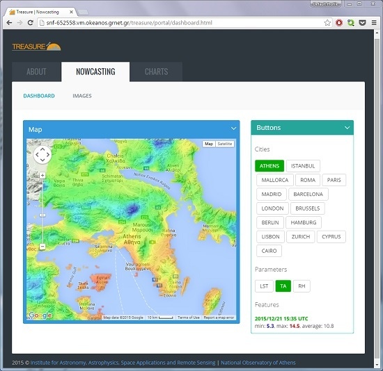
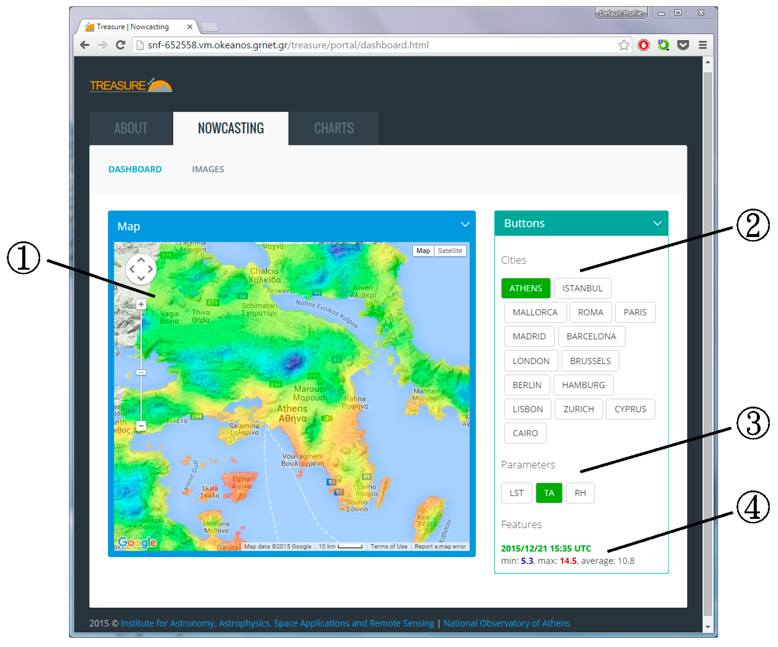
2.3.1. Nowcasting Dashboard
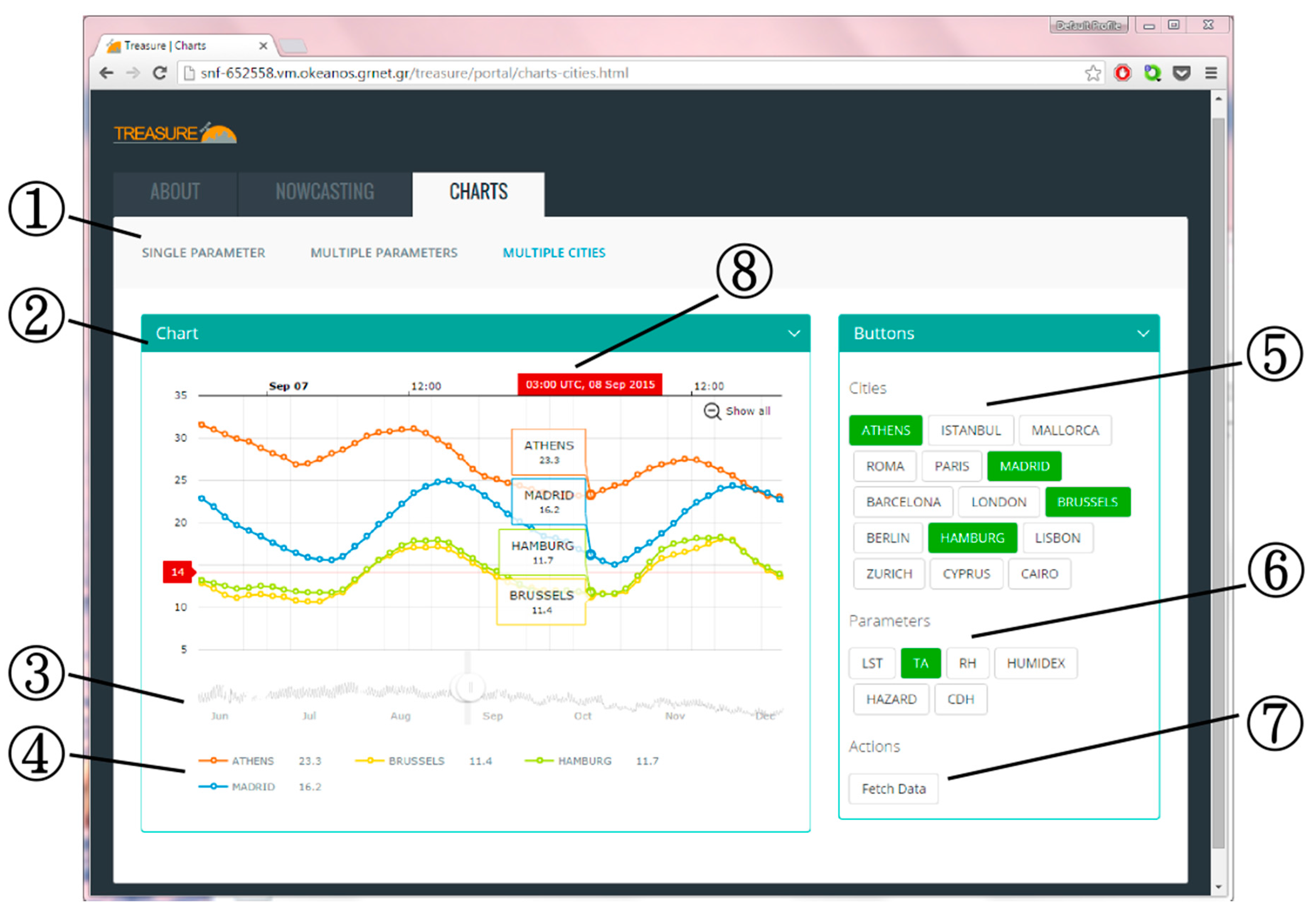
The nowcasting dashboard webpage (Figure 3) presents the most recently generated image for the city the user selected. The main element of the dashboard webpage is the map window (element ① in Figure 3) where the generated data are displayed using Google Maps as a basemap. The user can select the city and the surface parameter (elements ② and ③ in Figure 3, respectively). The requested image is loaded automatically and the user can use the Google Maps pan and zoom functions to examine it (only one image can be viewed at a time). The date and time (given in Coordinated Universal Time, UTC), as well as the minimum, average, and maximum values of the selected image is also presented for review by the user (element ④ in Figure 3). The color legend is normalized to this minimum-maximum range. The color of the date and time information are either green or red. Green indicates that the viewed image is the real-time SEVIRI satellite image (time difference between acquisition and availability of the system–timeliness-is less than 10 min), while red indicates a previously generated image is viewed. The lack of real-time data refers only to LST parameter and is related to non-availability due to cloud. TA is always available (green date and time stamp) as it presents the hybrid TA product (see Section 2.2).

2.3.2. Charts

The charts webpage presents the time series of the parameters extracted from the downscaled LST and TA products averaged over the urban areas. It offers three options to select from (element ① in Figure 4). The first option is to plot a single parameter for a single city, the second option is to plot multiple parameters for the same city, and the third option is to plot the same parameter for multiple cities. The graphical interface of the chart webpage is similar for these three options and is presented in Figure 4. The main element is the plot window (element ② in Figure 4), which is accompanied by a second plot presenting an overview of the entire time series (element ③ in Figure 4). The overview plot offers the function to scroll between dates and adjust the length of the time series viewed in the main window. The plot window also includes the plot legend, which corresponds to element ④ in Figure 4. The second part of the charts webpage is the feature selection window, which includes the city selection and the parameter selection menus (elements ⑤ and ⑥ in Figure 4, respectively). The first two chart types allow the selection of only one city while the third option allows the selection of multiple cities. For the desired parameters to be plotted in the chart window (element ② in Figure 4) the user has to confirm his/hers selection (element ⑦ in Figure 4). The resulted plotted curves correspond to the hourly average of each city urban areas. The chart’s graphical interface allows the user to view the values under the mouse cursor through the use of the dynamic labeling tool presented in Figure 4 as element ⑧.

3. Results of September 2015 Evaluation

In this section, the accuracy of the suggested method for TA estimation is analyzed for September 2015. To provide enough variety in the environmental conditions, all 15 cities presented in Figure 1 are included in the evaluation process. The selected regions are in different climatic zones, where the main climatic factor is either Mediterranean Sea (Cairo, Athens, Barcelona, Cyprus, Istanbul, Lisbon, Mallorca, and Rome), Atlantic Ocean (Brussels, Hamburg, London, and Paris), or the continental part of Europe (Berlin, Madrid, and Zurich).

3.1. In Situ TA Observations

The evaluation data, i.e., in-situ observations of TA, are available online at the National Oceanic and Atmospheric Administration (NOAA) archive (http://gis.ncdc.noaa.gov). In total, 96 stations are available for the 15 study areas. The in situ TA data have an hourly temporal resolution, thus only results that temporally fit best to the reference TA data have been considered. This means that the temporal difference between in situ and satellite observations is maximal 2.5 min.
Although the urban areas are the main focus of this work, other land cover types have also been included in the evaluation process (the land cover information was retrieved from the GlobCover dataset [57]). Specifically, from the available 96 stations, five stations were classified as water and three as open space and, thus, were ignored. The remaining 88 stations correspond either to rural (55 stations) or urban (33 stations) land cover types. The evaluation process also took into consideration the proximity to water. Specifically, two classes were defined from the 1 km pixels: the first class (28 stations) represents coastal pixels (not more than three 1 km pixels away from a water body, which corresponds approximately to one original SEVIRI pixel) and pixels that might partially include water bodies; while the second class (60 stations) represents inland pixels, i.e., pixels that are at least four pixels away from a water body. The third parameter considered is the elevation (retrieved from SRTM DEM [47]). In the global scale, most urban areas are situated in low elevations thus, the first class covers the elevation of not more than 100 m (50 stations) and the second one of all the rest (38 stations).
Here it should be also stressed that a comparison with in-situ observations is always difficult to interpret if the observed parameter is not homogenous within a satellite pixel. The uncertainties originate from inhomogeneous land surface, topography, soil moisture, possibly snow cover, etc. [58,59]. In addition, no knowledge of the TA source areas, i.e., the vicinity that influences in situ observations of TA [20,21], was available for this study.

3.2. Aggregated Results

Overall 40,085 observations were available for the 15 study areas. The accuracy over all areas is the following: Root Mean Square Error (RMSE) and Pearson’s correlation coefficient (Rho) have values of 2.3 °C and 0.95, respectively. Analysis of each area separately (Table 2) exposes some “problematic” areas like Cyprus and Zurich (Switzerland), but in general the accuracy is comparable or better than the accuracy in previous studies (in [29] an inherent error of 2 to 3 °C is reported).

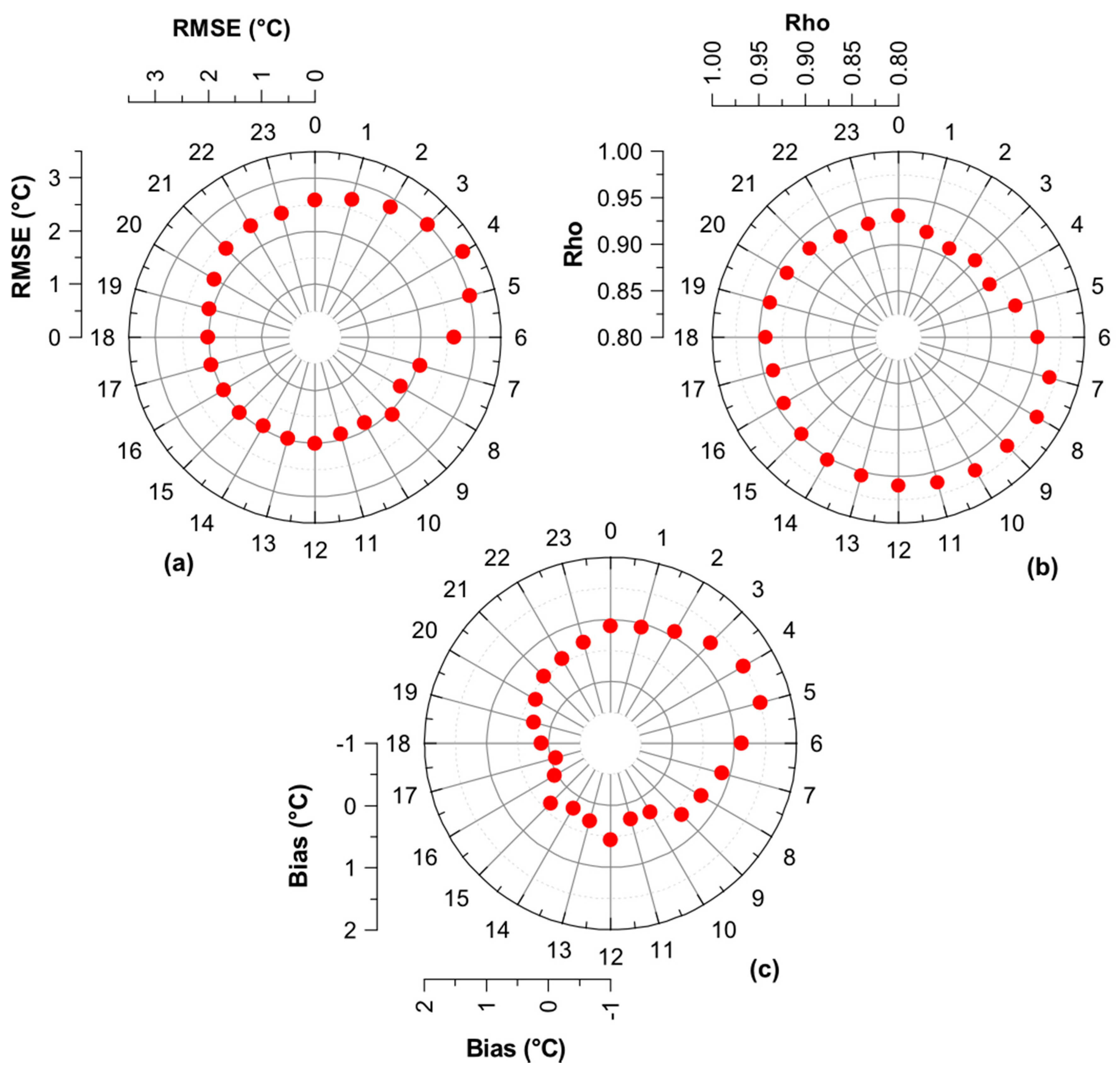
3.3. Diurnal Variation of Accuracy

Considering the high frequency of the employed data (5 min), the diurnal variation of the TA products’ accuracy was also considered. In average almost 1700 TA observations were available per hour. The calculated statistical measures are presented in the form of a polar plot, where the angle corresponds to UTC time (0–24), and the distance from the center to the value of the calculated statistical measure. Considering that data correspond to different time zones, the time should be recomputed to local solar time. However, the aggregated statistics do not change significantly using local time and, thus, the UTC time was retained.
Figure 5 presents the RMSE, Rho, and bias for each hour aggregated over all areas. The diurnal variation shows, that during daytime, RMSE is most of the time just below 2 °C, but its value rises during nighttime. Rho, on the other hand, is high during daytime, especially before noon as it reaches values over 0.97, but it drops down during the night to a lowest value of 0.85.

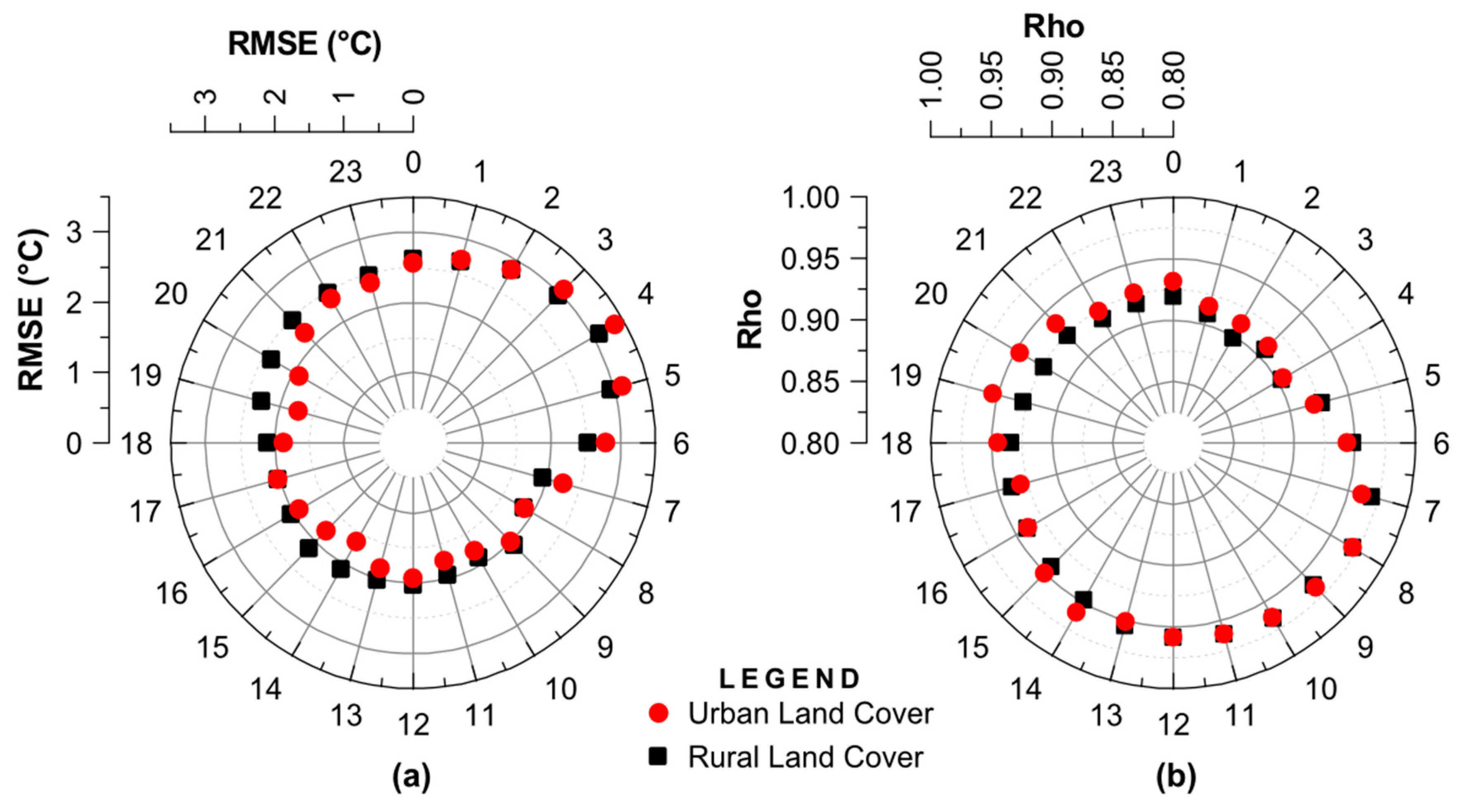
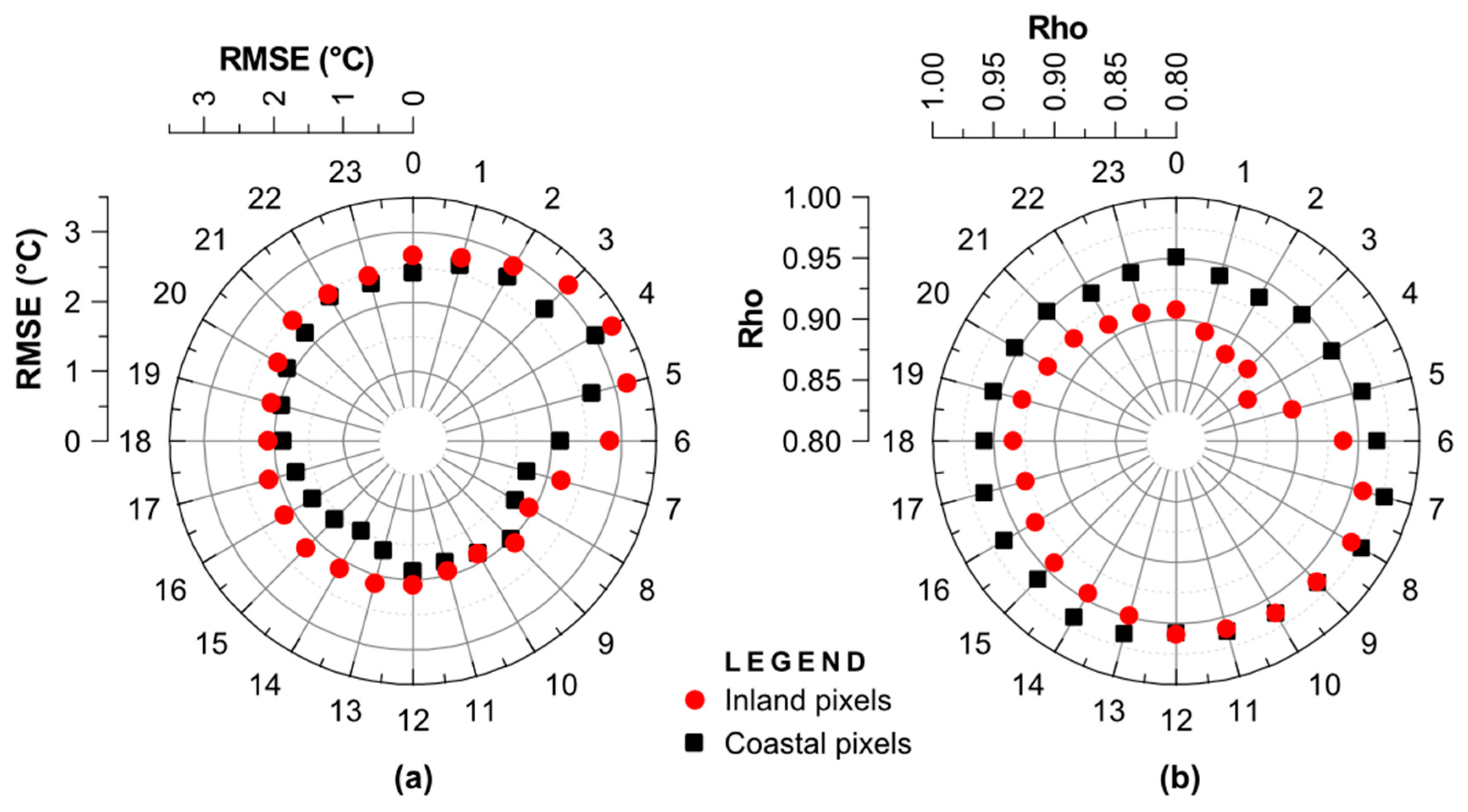
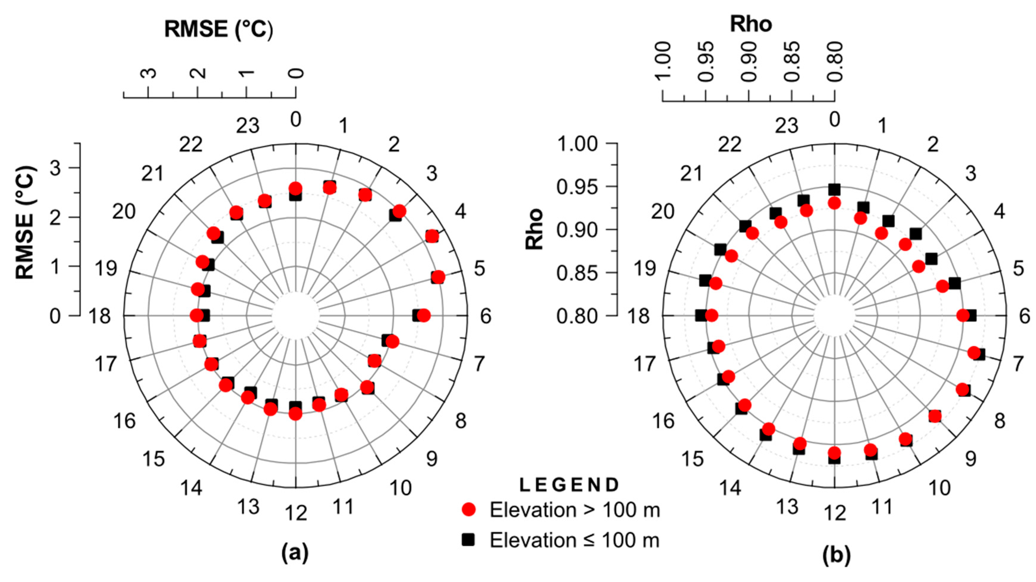
3.4. Diurnal Variation of Accuracy According to Different Location Classifications

Due to the interesting contrast in accuracy during nighttime and daytime, the diurnal variation of the accuracy according to land cover type was assessed next. The comparison between urban and rural land cover, which is presented in Figure 6, shows a similar trend as in Figure 5. There is no significant difference except in the late afternoon/early evening, as urban areas seem to have better accuracy. More systematic influence is seen when the stations are classified according to the distance to water (Figure 7). Areas closer to water seem to have better accuracy almost all day long except in the late morning. The highest accuracy (~1.5 °C) is achieved during the warmest hours of the day. However, the general trend is for both classes the same as for the whole dataset—better accuracy during daytime than during nighttime. The elevation also has a small, but a clear, influence on results (Figure 8). The lowest elevations, many of them are also close to sea, are more accurate almost each hour of a day. The difference of RMSE between the two classes shown in Figure 8 is never larger than 0.5 °C. However, the difference of Rho is higher especially during nighttime.

4. Discussion

Although some studies report a higher accuracy than this study does, this study covers urban characteristics in different climate zones, which has not been investigated adequately so far. For instance, Creswell [27] reached deviations smaller than 3 °C for 72% of the cases from Meteosat LST of Africa in November 1996 and June/July 1997. Jang et al. [28] multi-layer feed-forward neural networks resulted into a Rho of 0.93 and a RMSE of 1.8 °C. Zakšek et al. [29] set up a parameterization for Central Europe based on SEVIRI that resulted into a Rho of 0.95 and a RMSE of 2.0 °C. Pichierri et al. [24] used a split window approach to directly estimate canopy layer air temperatures for Milan (Italy) from the Moderate Resolution Imaging Spectroradiometer (MODIS) BTs, which yielded a RMSE of 1.8 °C for daytime data from May to September. Bechtel et al. [20] proposed a new approach based on multi-temporal geostationary LST data resulted in a RMSE of 1.8 °C, but they are valid only for six stations in Hamburg, Germany. TVX approach has usually a RMSE of 3–4 °C for AVHRR data [23,36]. Sun et al. [39] employed a surface energy balance approach and applied it for a region located in the North China Plain for two MODIS datasets (deviations smaller than 3 °C for 80% of the cases). Ho et al. [33] used an advanced statistical approach to map Vancouver’s (Canada) maximum urban TA using Landsat data with a RMSE of 2.3 °C, while Kloog et al. [26,30] assessed the minimum and mean TA for Massachusetts (USA) using MODIS data and achieved a R2 equal to 0.95. Shi et al. [32] extended the hybrid statistical model presented by Klogg et al. [26,30] and estimated the 15-year daily local air temperature in the Southeastern USA with a R2 equal to 0.95. Nichol and To [35] estimated the daytime and nighttime TA for Kowloon Peninsula in Hong Kong using ASTER data and achieved a R2 equal to 0.75 and a mean absolute difference (MAD) of 3.57 °C for daytime, and a R2 equal to 0.84 and a MAD of 1.4 °C, for nighttime.
In this study, only Cyprus and Zurich (Switzerland) areas had a RMSE worse than 3 °C (Table 2). The most probable explanation for such deviation is documented in the SPhR algorithm manual [42]: the SPhR algorithm can exhibit large errors over mountain regions with large differences between the topography and the NWP topography. In both areas, mountains with an altitude of about 2000 m are present. Temperature profiles in such areas and also in their surroundings significantly differ than free atmosphere profiles. Considering the cities in mostly flat areas, e.g., London (United Kingdom) or Hamburg (Germany), this statement is supported—the areas without any significant topography have the lowest RMSEs. The only example might be Paris, whose RMSE reaches 2.3 °C, which, nonetheless, is still a reliable value.
The analysis of diurnal variation of accuracy revealed a great potential to increase accuracy, because a significant bias was observed during nighttime. A bias is usually a result of a systematic error. To address this issue, the difference of the processes that define TA during daytime and nighttime have to be considered. During daytime, the air is heated indirectly through the incoming solar energy heating the surface. The net radiation is positive, thus the surface warms up. Part of the heat is radiated into the atmosphere, which warms up as well. The relationship between surface and TA depends on the Bowen ratio, which describes the partitioning of net radiation into latent and sensible heat. During the nighttime, the net radiation is negative, thus the surface cools down. Kawashima et al. [60] explained that ~80% of the variance in the night temperature is explained by the surface temperature. A large part of the remaining variation depends on the wind speed. Therefore, the processes that control the TA are significantly different during daytime and nighttime.
In this study, a single parameterization—independent of time—is employed. The primal suspect for the observed nighttime positive bias is the temperature inversion. In most of the September case studies nights were clear and calm. These conditions are perfect for creating inversions near the ground. In such situations, the ground—which cools quicker than the air in the atmosphere—cools the overlaying above-ground atmospheric air layer. However in the higher atmospheric layers, the air cools slower than in the layers close to the ground. This creates a so called “nocturnal thermal inversion”, which can be also observed in early mornings [61]. This effect is confined mostly to land regions, as the ocean retains heat far longer.
As the SPhR algorithm [42] expects a constantly decreasing temperature with increasing height, the error is possible at calm and clear night. The areas close to the ground, where TA is measured, are cooler than a higher atmosphere layer. This means that the real atmospheric profile of the temperature deviates from our profile in the layers close to the ground. The SPhR assumes that the lowest layer is the warmest, but this is not the case during a nocturnal thermal inversion. Thus, the estimated values are larger than the in situ observations.

5. Conclusions

The IAASARS/NOA nowcasting module for generating high spatiotemporal TA data (1 km/5 min) is freely accessible at http://snf-652558.vm.okeanos.grnet.gr/treasure/portal/info.html. The spatiotemporal characteristics of the presented products are unique and can capture the diurnal spatial variability of urban temperatures, which has been inadequate in previous urban climate studies. Overall, the system’s timeliness (10 min), online operation, real-time capability, and capacity to cover numerous cities, offers a stable basis for the development of numerous applications related to energy demand, urban planning, smart cities, and heatwave monitoring, and enables the establishment of synergies with other data sources and disciplines.
The TA evaluation showed that its RMSE and Rho are 2.3 °C and 0.95, respectively, which is comparable to, or better than, previous studies. The diurnal analysis shows that the TA module operates better during daytime than nighttime. Furthermore, better estimates are expected in flat regions than in mountainous regions. The evaluation process revealed a high positive bias during nighttime, which is most probably due to the improper handling of the nocturnal thermal inversion by the TA module. The nighttime bias can reach +2 °C for urban areas. This means, that the proposed approach, although it already achieves good statistics, can be further improved, once this bias is eliminated. Presently, the TA module continues operation and populates each city’s database (a several-year-long time series will further enable the estimation of TA trends). Future work should focus on the compensation of the nighttime bias and the evaluation of the TA module for a longer time period so as to assess its performance with respect to seasons.

Acknowledgments

EUMETSAT is the source of the original Meteosat Images. The MSG-SEVIRI data were acquired by the EUMETCast station operated by the Institute for Astronomy, Astrophysics, Space Application and Remote Sensing of the National Observatory of Athens. This publication was supported by (i) the Humanitarian Aid and Civil Protection Department of the European Commission in the framework of the project TREASURE, under Grant Agreement No. 695561 (TREASURE—Thermal Risk Reduction Actions and Tools for Secure Cities); (ii) the European Union Seventh Framework Programme (FP7-REGPOT-2012-2013-1), in the framework of the project BEYOND, under Grant Agreement No. 316210 (BEYOND—Building Capacity for a Centre of Excellence for EO-based monitoring of Natural Disasters); (iii) the “Development Proposals of Research Entities—KRIPIS”, which is funded by N.P. “Competitiveness and Entrepreneurship”, Action: “PROTEAS—Advanced Space Applications for the Exploration of the Universe, Space and Earth”; and (iv) the Excellence Research Programme GSRT (2015–2017) ARISTOTELIS “Environment, Space and Geodynamics/Seismology 2015-2017”.

Author Contributions

I.K. and C.T.K. devised, designed, and implemented the module presented and wrote parts of the paper. P.S. wrote parts of the paper and prepared the figures. K.Z. performed the comparison with the in-situ data, analyzed the results and wrote parts of the paper. All authors reviewed the manuscript.

Conflicts of Interest

The authors declare no conflict of interest.

Abbreviations

The following abbreviations are used in this manuscript:
ASTERAdvanced Spaceborne Thermal Emission and Reflection Radiometer
AVHRRAdvanced Very High Resolution Radiometer
BTBrightness Temperature
CMaCloud Mask
DEM Digital Elevation Model
DLSTDownscaled Land Surface Temperature
EUMETSATEuropean Organization for the Exploitation of Meteorological Satellites
FORField-of-Regard
GFSGlobal Forecasting System
GRIBGridded Binary
HRVHigh Resolution Visible
IAASARS/NOAInstitute for Astronomy, Astrophysics, Space Applications and Remote Sensing of the National Observatory of Athens
LSTLand Surface Temperature
MADMean Absolute Difference
MODISModerate Resolution Imaging Spectroradiometer
MSG-SEVIRIMeteosat Second Generation—Spinning Enhanced Visible and Infrared Imager
NCEPNational Centers for Environmental Prediction
NDVINormalized Difference Vegetation Index
NOAANational Oceanic and Atmospheric Administration
NWPNumerical Weather Predictions
RhoPearson’s Correlation Coefficient
RMSERoot Mean Square Error
RSSRapid Scan System
RTRadiative Transfer
RTTOVRadiative Transfer for TIROS (Television Infrared Observation Satellite) Operational Vertical Sounder
SAFNWCSatellite Application Facility for Nowcasting Weather Conditions Software
SPhRSAFNWC’s Physical Retrieval Algorithm
SRTMShuttle Radar Topography Mission
SZASolar Zenith Angle
TAAir Temperature at 2 m Height
TIRThermal Infrared Radiation
TVXTemperature-Vegetation Index
UHIUrban Heat Island
UTCCoordinated Universal Time

References

  1. United Nations. World Urbanization Prospects: The 2014 Revision, Highlights (ST/ESA/SER.A/352); United Nations: New York, NY, USA, 2014. [Google Scholar]
  2. Schneider, A.; Friedl, M.A.; Potere, D. Mapping Global Urban Areas Using MODIS 500-M Data: New Methods and Datasets Based on “urban Ecoregions”. Remote Sens. Environ. 2010, 114, 1733–1746. [Google Scholar] [CrossRef]
  3. Oke, T. The Energetic Basis of the Urban Heat Island. Q. J. R. Meteorol. Soc. 1982, 108, 1–24. [Google Scholar] [CrossRef]
  4. Akbari, H.; Davis, S.; Dorsano, S.; Huang, J.; Winnett, S. Cooling Our Communities a Guidebook on Tree Planting and Light-Colored Surfacing; EPA: Washington, DC, USA, 1992. [Google Scholar]
  5. Rizwan, A.M.; Dennis, L.Y.C.; Liu, C. A Review on the Generation, Determination and Mitigation of Urban Heat Island. J. Environ. Sci. 2008, 20, 120–128. [Google Scholar] [CrossRef]
  6. Ding, B.; Rosenfeld, A.H.; Akbari, H.; Bretz, S.; Fishman, B.L.; Kurn, D.M.; Sailor, D.; Taha, H. Mitigation of Urban Heat Islands: Materials, Utility Programs, Updates. Energy Build. 1995, 22, 255–265. [Google Scholar]
  7. Tan, J.; Zheng, Y.; Tang, X.; Guo, C.; Li, L.; Song, G.; Zhen, X.; Yuan, D.; Kalkstein, A.J.; Li, F. The Urban Heat Island and Its Impact on Heat Waves and Human Health in Shanghai. Int. J. Biometeorol. 2010, 54, 75–84. [Google Scholar] [CrossRef] [PubMed]
  8. Lo, C.P.; Quattrochi, D.A. Land-Use and Land-Cover Change, Urban Heat Island Phenomenon, and Health Implications: A Remote Sensing Approach. Photogramm. Eng. Remote Sens. 2003, 69, 1053–1063. [Google Scholar] [CrossRef]
  9. Kolokotroni, M.; Ren, X.; Davies, M.; Mavrogianni, A. London’s Urban Heat Island: Impact on Current and Future Energy Consumption in Office Buildings. Energy Build. 2012, 47, 302–311. [Google Scholar] [CrossRef]
  10. Basu, R. High Ambient Temperature and Mortality: A Review of Epidemiologic Studies from 2001 to 2008. Environ. Heal. 2009, 8, 40. [Google Scholar] [CrossRef] [PubMed]
  11. Ho, H.C.; Knudby, A.; Xu, Y.; Hodul, M.; Aminipouri, M. A Comparison of Urban Heat Islands Mapped Using Skin Temperature, Air Temperature, and Apparent Temperature (Humidex), for the Greater Vancouver Area. Sci. Total Environ. 2015, 544, 929–938. [Google Scholar] [CrossRef] [PubMed]
  12. Ho, H.; Knudby, A.; Huang, W. A Spatial Framework to Map Heat Health Risks at Multiple Scales. Int. J. Environ. Res. Public Health 2015, 12, 16110–16123. [Google Scholar] [CrossRef] [PubMed]
  13. Kloog, I.; Melly, S.J.; Coull, B.A.; Nordio, F.; Schwartz, J.D. Satellite-Based Spatiotemporal Resolved Air Temperature Exposure to Study the Association between Ambient Air Temperature and Birth Outcomes in Massachusetts. Environ. Health Perspect. 2015, 123, 1053–1058. [Google Scholar] [CrossRef] [PubMed]
  14. Kovats, R.S.; Hajat, S. Heat Stress and Public Health: A Critical Review. Annu. Rev. Public Health 2008, 29, 41–55. [Google Scholar] [CrossRef] [PubMed]
  15. Lai, P.-C.; Choi, C.C.Y.; Wong, P.P.Y.; Thach, T.-Q.; Wong, M.S.; Cheng, W.; Krämer, A.; Wong, C.-M. Spatial Analytical Methods for Deriving a Historical Map of Physiological Equivalent Temperature of Hong Kong. Build. Environ. 2016, 99, 22–28. [Google Scholar] [CrossRef]
  16. Shi, L.; Kloog, I.; Zanobetti, A.; Liu, P.; Schwartz, J.D. Impacts of Temperature and Its Variability on Mortality in New England. Nat. Clim. Chang. 2015, 5, 1–5. [Google Scholar] [CrossRef] [PubMed]
  17. Bechtel, B.; Zakšek, K.; Hoshyaripour, G. Downscaling Land Surface Temperature in an Urban Area: A Case Study for Hamburg, Germany. Remote Sens. 2012, 4, 3184–3200. [Google Scholar] [CrossRef]
  18. Nichol, J.E.; Wong, M.S. Spatial Variability of Air Temperature and Appropriate Resolution for Satellite-Derived Air Temperature Estimation. Int. J. Remote Sens. 2008, 29, 7213–7223. [Google Scholar] [CrossRef]
  19. Voogt, J.A.; Oke, T. Thermal Remote Sensing of Urban Climates. Remote Sens. Environ. 2003, 86, 370–384. [Google Scholar] [CrossRef]
  20. Bechtel, B.; Wiesner, S.; Zaksek, K. Estimation of Dense Time Series of Urban Air Temperatures from Multitemporal Geostationary Satellite Data. IEEE J. Sel. Top. Appl. Earth Obs. Remote Sens. 2014, 7, 1–9. [Google Scholar] [CrossRef]
  21. Zakšek, K.; Bechtel, B. Source Area Estimation of Urban Air Temperatures. In Joint Urban Remote Sensing Event 2015; IEEE: Lausanne, Switzerland, 2015; pp. 1–4. [Google Scholar]
  22. Ken Parsons. Human Thermal Environments: The Effects of Hot, Moderate, and Cold Environments on Human Health, Comfort, and Performance, Third Edit. ed; CRC Press: Boca Raton, FL, USA, 2014. [Google Scholar]
  23. Prihodko, L.; Goward, S. Estimation of Air Temperature from Remotely Sensed Surface Observations. Remote Sens. Environ. 1997, 4257, 335–346. [Google Scholar] [CrossRef]
  24. Pichierri, M.; Bonafoni, S.; Biondi, R. Satellite Air Temperature Estimation for Monitoring the Canopy Layer Heat Island of Milan. Remote Sens. Environ. 2012, 127, 130–138. [Google Scholar] [CrossRef]
  25. Fung, W.Y.; Lam, K.S.; Nichol, J.; Wong, M.S. Derivation of Nighttime Urban Air Temperatures Using a Satellite Thermal Image. J. Appl. Meteorol. Climatol. 2009, 48, 863–872. [Google Scholar] [CrossRef]
  26. Kloog, I.; Chudnovsky, A.; Koutrakis, P.; Schwartz, J. Temporal and Spatial Assessments of Minimum Air Temperature Using Satellite Surface Temperature Measurements in Massachusetts, USA. Sci. Total Environ. 2012, 432, 85–92. [Google Scholar] [CrossRef] [PubMed]
  27. Cresswell, M.P.; Morse, A.P.; Thomson, M.C.; Connor, S.J. Estimating Surface Air Temperatures, from Meteosat Land Surface Temperatures, Using an Empirical Solar Zenith Angle Model. Int. J. Remote Sens. 1999, 20, 1125–1132. [Google Scholar] [CrossRef]
  28. Jang, J.-D.; Viau, A.A.; Anctil, F. Neural Network Estimation of Air Temperatures from AVHRR Data. Int. J. Remote Sens. 2004, 25, 4541–4554. [Google Scholar] [CrossRef]
  29. Zakšek, K.; Schroedter-Homscheidt, M. Parameterization of Air Temperature in High Temporal and Spatial Resolution from a Combination of the SEVIRI and MODIS Instruments. ISPRS J. Photogramm. Remote Sens. 2009, 64, 414–421. [Google Scholar] [CrossRef]
  30. Kloog, I.; Nordio, F.; Coull, B.A.; Schwartz, J. Predicting Spatiotemporal Mean Air Temperature Using MODIS Satellite Surface Temperature Measurements across the Northeastern USA. Remote Sens. Environ. 2014, 150, 132–139. [Google Scholar]
  31. Zeng, L.; Wardlow, B.; Tadesse, T.; Shan, J.; Hayes, M.; Li, D.; Xiang, D. Estimation of Daily Air Temperature Based on MODIS Land Surface Temperature Products over the Corn Belt in the US. Remote Sens. 2015, 7, 951–970. [Google Scholar]
  32. Shi, L.; Liu, P.; Kloog, I.; Lee, M.; Kosheleva, A.; Schwartz, J. Estimating Daily Air Temperature across the Southeastern United States Using High-Resolution Satellite Data: A Statistical Modeling Study. Environ. Res. 2016, 146, 51–58. [Google Scholar]
  33. Ho, H.C.; Knudby, A.; Sirovyak, P.; Xu, Y.; Hodul, M.; Henderson, S.B. Mapping Maximum Urban Air Temperature on Hot Summer Days. Remote Sens. Environ. 2014, 154, 38–45. [Google Scholar]
  34. Anniballe, R.; Bonafoni, S.; Pichierri, M. Spatial and Temporal Trends of the Surface and Air Heat Island over Milan Using MODIS Data. Remote Sens. Environ. 2014, 150, 163–171. [Google Scholar]
  35. Nichol, J.E.; To, P.H. Temporal Characteristics of Thermal Satellite Images for Urban Heat Stress and Heat Island Mapping. ISPRS J. Photogramm. Remote Sens. 2012, 74, 153–162. [Google Scholar]
  36. Czajkowski, K.; Goward, S.; Stadler, S.; Walz, A. Thermal Remote Sensing of Near Surface Environmental Variables: Application Over the Oklahoma Mesonet. Prof. Geogr. 2000, 52, 345–357. [Google Scholar]
  37. Prince, S.D.; Goetz, S.J.; Dubayah, R.O.; Czajkowski, K.P.; Thawley, M. Inference of Surface and Air Temperature, Atmospheric Precipitable Water and Vapor Pressure Deficit Using Advanced Very High-Resolution Radiometer Satellite Observations: Comparison with Field Observations. J. Hydrol. 1998, 212–213, 230–249. [Google Scholar]
  38. Pape, R.; Löffler, J. Modelling Spatio-Temporal near-Surface Temperature Variation in High Mountain Landscapes. Ecol. Model. 2004, 178, 483–501. [Google Scholar]
  39. Sun, Y.J.; Wang, J.F.; Zhang, R.H.; Gillies, R.R.; Xue, Y.; Bo, Y.C. Air Temperature Retrieval from Remote Sensing Data Based on Thermodynamics. Theor. Appl. Climatol. 2005, 80, 37–48. [Google Scholar]
  40. Weng, Q. Thermal Infrared Remote Sensing for Urban Climate and Environmental Studies: Methods, Applications, and Trends. ISPRS J. Photogramm. Remote Sens. 2009, 64, 335–344. [Google Scholar]
  41. Fernandez, P. Software User Manual for the SAFNWC/MSG Application: Software Part (SAF/NWC/CDOP/INM/SW/SUM/2); Technical Report; EUMETSAT NWC SAF: Madrid, Spain, 2012. [Google Scholar]
  42. Martinez, M.A.; Manso, M.; Fernández, P. Algorithm Theoretical Basis Document for “SEVIRI Physical Retrieval” (SPhR-PGE13 v2.0); Technical Report; EUMETSAT NWC SAF: Madrid, Spain, 2013. [Google Scholar]
  43. Sismanidis, P.; Keramitsoglou, I.; Kiranoudis, C.T. A Satellite-Based System for Continuous Monitoring of Surface Urban Heat Islands. Urban Clim. 2015, 14, 141–153. [Google Scholar]
  44. Sismanidis, P.; Keramitsoglou, I.; Kiranoudis, C.T. Evaluating the Operational Retrieval and Downscaling of Urban Land Surface Temperatures. IEEE Geosci. Remote Sens. Lett. 2015, 12, 1312–1316. [Google Scholar]
  45. Global Climate and Weather Modeling Branch. The GFS Atmospheric Model—NCEP Office Note 442; Global Climate and Weather Modeling Branch: Camp Springs, MD, USA, 2003. [Google Scholar]
  46. Keramitsoglou, I.; Kiranoudis, C.T.; Weng, Q. Downscaling Geostationary Land Surface Temperature Imagery for Urban Analysis. IEEE Geosci. Remote Sens. Lett. 2013, 10, 1253–1257. [Google Scholar]
  47. Rabus, B.; Eineder, M.; Roth, A.; Bamler, R. The Shuttle Radar Topography Mission—A New Class of Digital Elevation Models Acquired by Spaceborne Radar. ISPRS J. Photogramm. Remote Sens. 2003, 57, 241–262. [Google Scholar]
  48. Derrien, M.; Le Gléau, H.; Fernandez, P. Algorithm Theoretical Basis Document for Cloud Products (CMa-PGE01 v3.2, CT-PGE02 v2.2 & CTTH-PGE03 v2.2); Technical Report; EUMETSAT NWC SAF: Madrid, Spain, 2013. [Google Scholar]
  49. Derrien, M.; Le Gléau, H. MSG/SEVIRI Cloud Mask and Type from SAFNWC. Int. J. Remote Sens. 2005, 26, 4707–4732. [Google Scholar]
  50. Derrien, M.; Le Gléau, H.; Fernandez, P. Validation Report for “Cloud Products” (CMa-PGE01 v3.2, CT-PGE02 v2.2 & CTTH-PGE03 v2.2); Technical Report; EUMETSAT NWC SAF: Madrid, Spain, 2013. [Google Scholar]
  51. Liou, K.N. An Introduction to Atmospheric Radiation, 2nd ed.; Academic Press: San Diego, CA, USA, 2002. [Google Scholar]
  52. Saunders, R. RTTOV-9 Users Guide; EUMETSAT NWP SAF: Exeter, UK, 2010. [Google Scholar]
  53. Bonnans, J.F.; Gilbert, J.C.; Lemaréchal, C.; Sagastizábal, C.A. Numerical Optimization, Theoretical and Numerical Aspects, Second Ed. ed; Springer: Berlin, German, 2006. [Google Scholar]
  54. Berberan-Santos, M.N.; Bodunov, E.N.; Pogliani, L. On the Barometric Formula. Am. J. Phys. 1997, 65, 404. [Google Scholar]
  55. Wilson, D.C.; Mair, B.A. Thin-Plate Spline Interpolation. In Sampling, Wavelets, and Tomography; Birkhäuser: Boston, MA, USA, 2004; pp. 311–340. [Google Scholar]
  56. Zakšek, K.; Oštir, K. Downscaling Land Surface Temperature for Urban Heat Island Diurnal Cycle Analysis. Remote Sens. Environ. 2012, 117, 114–124. [Google Scholar] [CrossRef]
  57. Arino, O.; Gross, D.; Ranera, F.; Bourg, L.; Leroy, M.; Bicheron, P.; Latham, J.; Di Gregorio, A.; Brockman, C.; Witt, R.; et al. GlobCover: ESA Service for Global Land Cover from MERIS. In Geoscience and Remote Sensing Symposium; IEEE: Barcelona, Spain, 2007; pp. 2412–2415. [Google Scholar]
  58. Keramitsoglou, I.; Daglis, I.A.; Amiridis, V.; Chrysoulakis, N.; Ceriola, G.; Manunta, P.; Maiheu, B.; De Ridder, K.; Lauwaet, D.; Paganini, M. Evaluation of Satellite-Derived Products for the Characterization of the Urban Thermal Environment. J. Appl. Remote Sens. 2012, 6, 061704. [Google Scholar] [CrossRef]
  59. Urban, M.; Eberle, J.; Hüttich, C.; Schmullius, C.; Herold, M. Comparison of Satellite-Derived Land Surface Temperature and Air Temperature from Meteorological Stations on the Pan-Arctic Scale. Remote Sens. 2013, 5, 2348–2367. [Google Scholar] [CrossRef]
  60. Kawashima, S.; Ishida, T.; Minomura, M.; Miwa, T. Relations between Surface Temperature and Air Temperature on a Local Scale during Winter Nights. J. Appl. Meteorol. 2000, 39, 1570–1579. [Google Scholar] [CrossRef]
  61. Surridge, A.D. Extrapolation of the Nocturnal Temperature Inversion from Ground-Based Measurements. Atmos. Environ. 1986, 20, 803–806. [Google Scholar] [CrossRef]
Figure 1. The cities covered by the IAASARS/NOA service since June 2015.
Remotesensing 08 00306 g001
Figure 2. The 12:00 UTC TA products for (a) 5th and (b) 6th of September 2015 for the city of Athens, Greece. During these two days the last heatwave of Athens for summer 2015 took place (6 September was the hottest day of the heatwave). The comparison of the two maps reveals the increase of the TA values and the intensification of Athens’ UHI as captured by IAASARS/NOA system.
Remotesensing 08 00306 g002
Figure 3. The graphical interface of the nowcasting dashboard webpage. ① is the map window; ② is the city selection menu; ③ is the parameter selection menu (e.g., LST, TA or RH); and ④ is the displayed image legend that presents information about the date and time of the SEVIRI image acquisition and the min/max/average value of the selected parameter.
Remotesensing 08 00306 g003
Figure 4. The graphical interface of the charts/multiple cities webpage. ① is the chart type selection menu; ② is the chart display window; ③ is an overview of the selected time series; ④ is the chart legend; ⑤ is the city selection menu; ⑥ is the parameter selection menu; ⑦ is the action button for plotting the selected parameters; and ⑧ is a dynamic label presenting the date, time, and parameter values for the plot point closest to the mouse cursor.
Remotesensing 08 00306 g004
Figure 5. The diurnal variation of TA (a) RMSE; (b) Rho; and (c) bias for all observations.
Remotesensing 08 00306 g005
Figure 6. The diurnal variation of TA (a) RMSE and (b) Rho for urban and rural pixels.
Remotesensing 08 00306 g006
Figure 7. The diurnal variation of TA (a) RMSE and (b) Rho for inland and coastal pixels.
Remotesensing 08 00306 g007
Figure 8. The diurnal variation of TA (a) RMSE and (b) Rho for pixels with an elevation greater than 100 m and less or equal than 100 m.
Remotesensing 08 00306 g008
Table 1. The required GFS NWP short-term forecasts for the generation of the SAFNWC CMa and SPhR products [42,48].
GFS NWP Forecast DataCMaSPhR
Skin TemperatureXX
Surface Pressure-X
Atmospheric Water Vapour ContentX-
Temperature at various levels *XX
Humidity at various levels *-X
NWP altitude modelX-
NWP landseaX-
Geopotential at surfaceX-
* Pressure levels (hPa): 1000, 925, 850, 700, 500, 400, 300, 250, 200, 150, 100, 70, 50, 30, 10.
Table 2. The RMSE and Rho values for each study area.
Study AreaRMSE (°C)RhoStudy AreaRMSE (°C)Rho
Athens2.20.90Lisbon1.60.91
Barcelona1.90.87London1.70.86
Berlin1.70.92Madrid2.60.91
Brussels1.40.90Mallorca *2.20.89
Cairo2.10.94Paris2.30.78
Cyprus *3.00.82Rome2.50.91
Hamburg1.60.84Zurich3.10.79
Istanbul2.10.83Total2.30.95
* The TA product depicts the entire island of Cyprus/Mallorca and not only the main urban agglomeration. The reported statistical measures have been calculated by aggregating the in situ observations from all meteorological station situated in each island.

