
Testing the Contribution of Stress Factors to Improve Wheat and Maize Yield Estimations Derived from Remotely-Sensed Dry Matter Productivity


 , and
, and
Abstract
:
1. Introduction
2. Materials
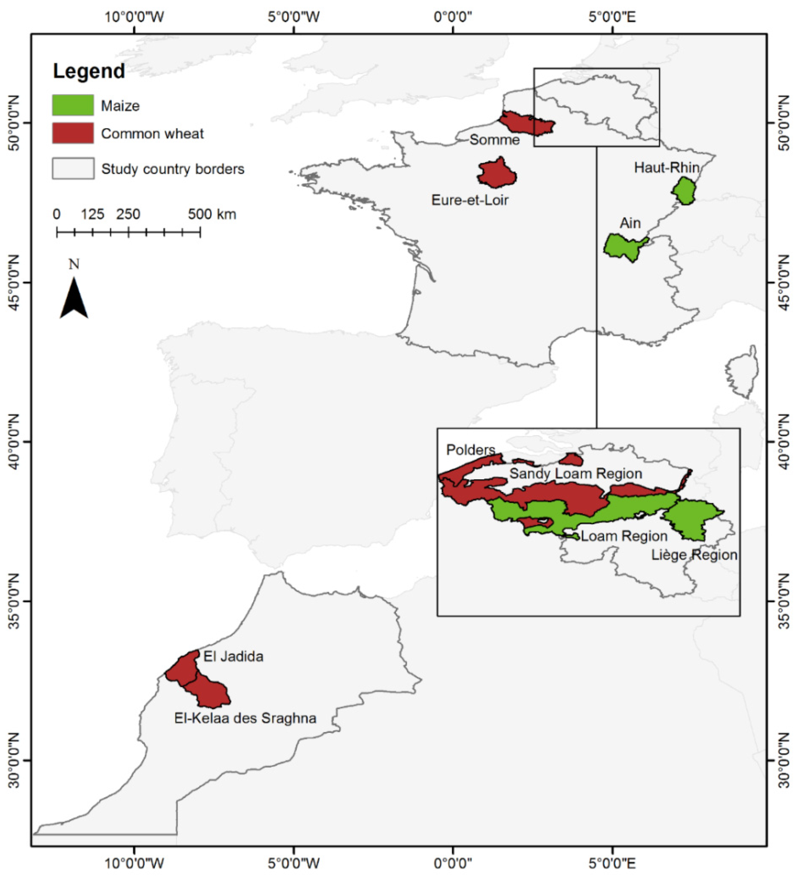
2.1. Study Areas and Crops
2.2. Data Description
3. Methods
3.1. Algorithm Description of the DMP Model
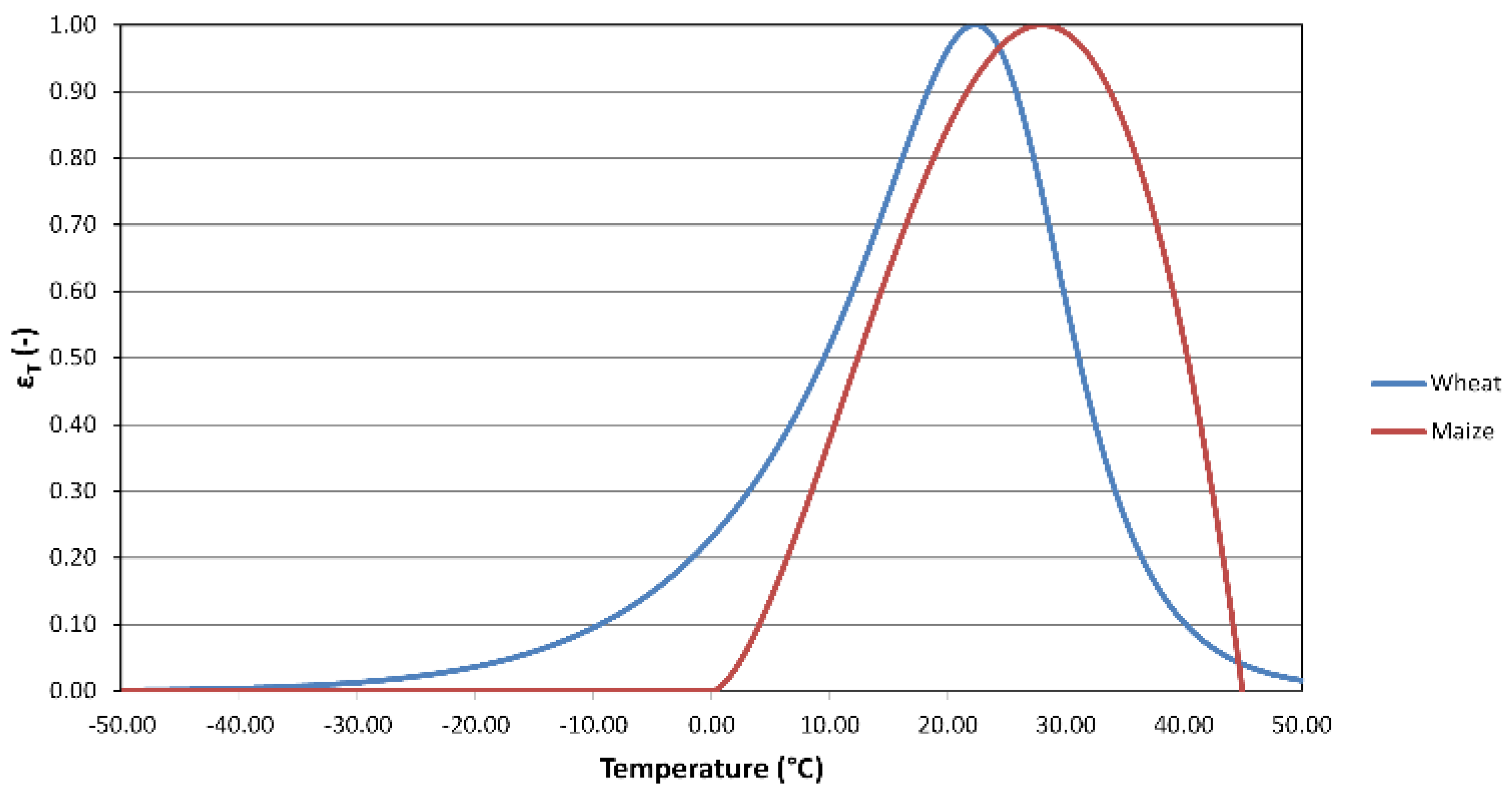
3.1.1. Temperature Stress Factor
3.1.2. CO2 Fertilisation Effect
3.1.3. Water Stress Factor
3.1.4. Autotrophic Respiration Factor
3.2. Regression Analysis
4. Results
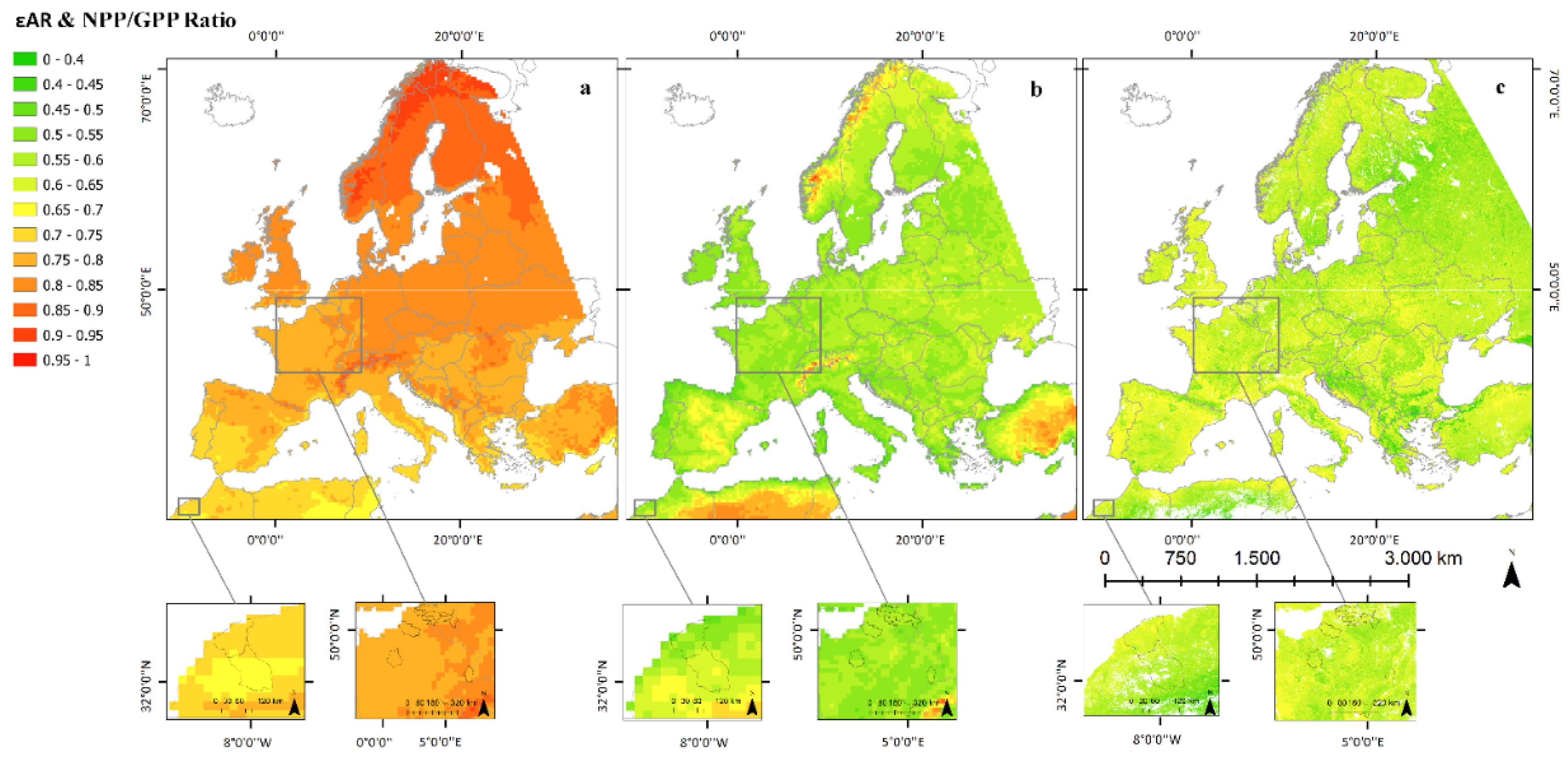
4.1. Autotrophic Respiration Fraction (εAR)
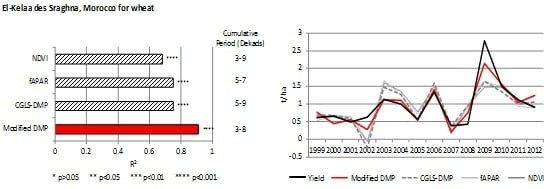
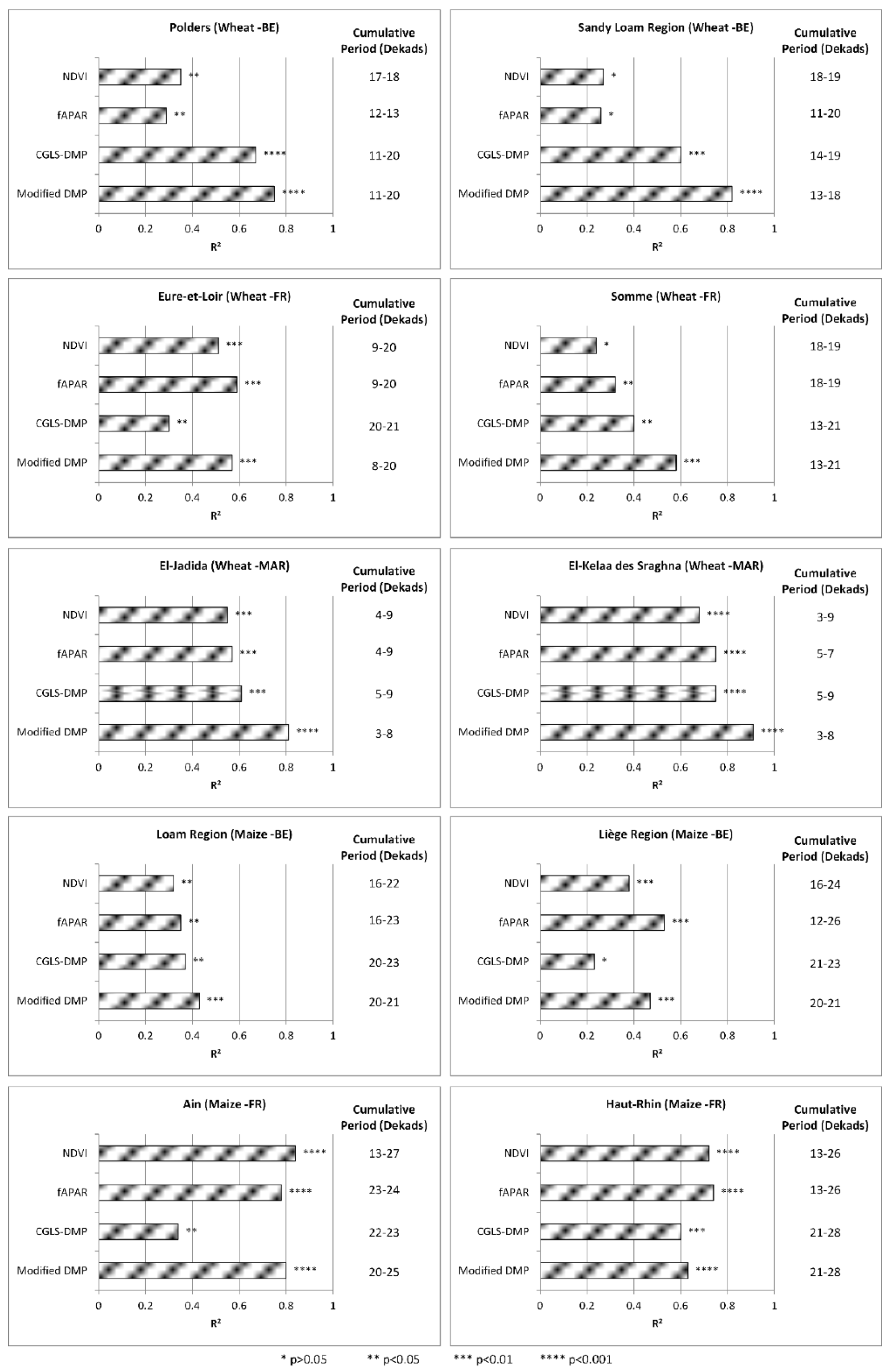
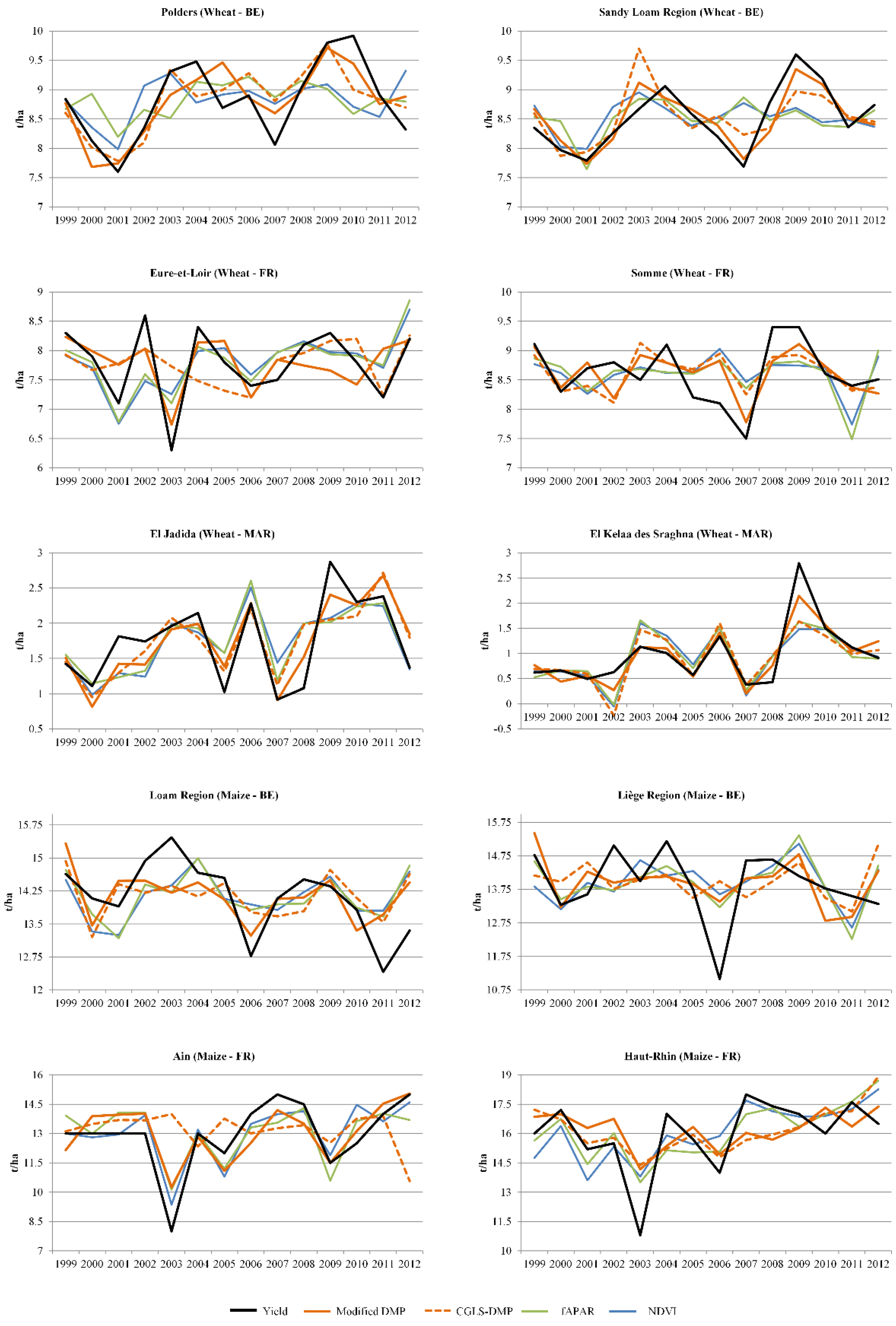
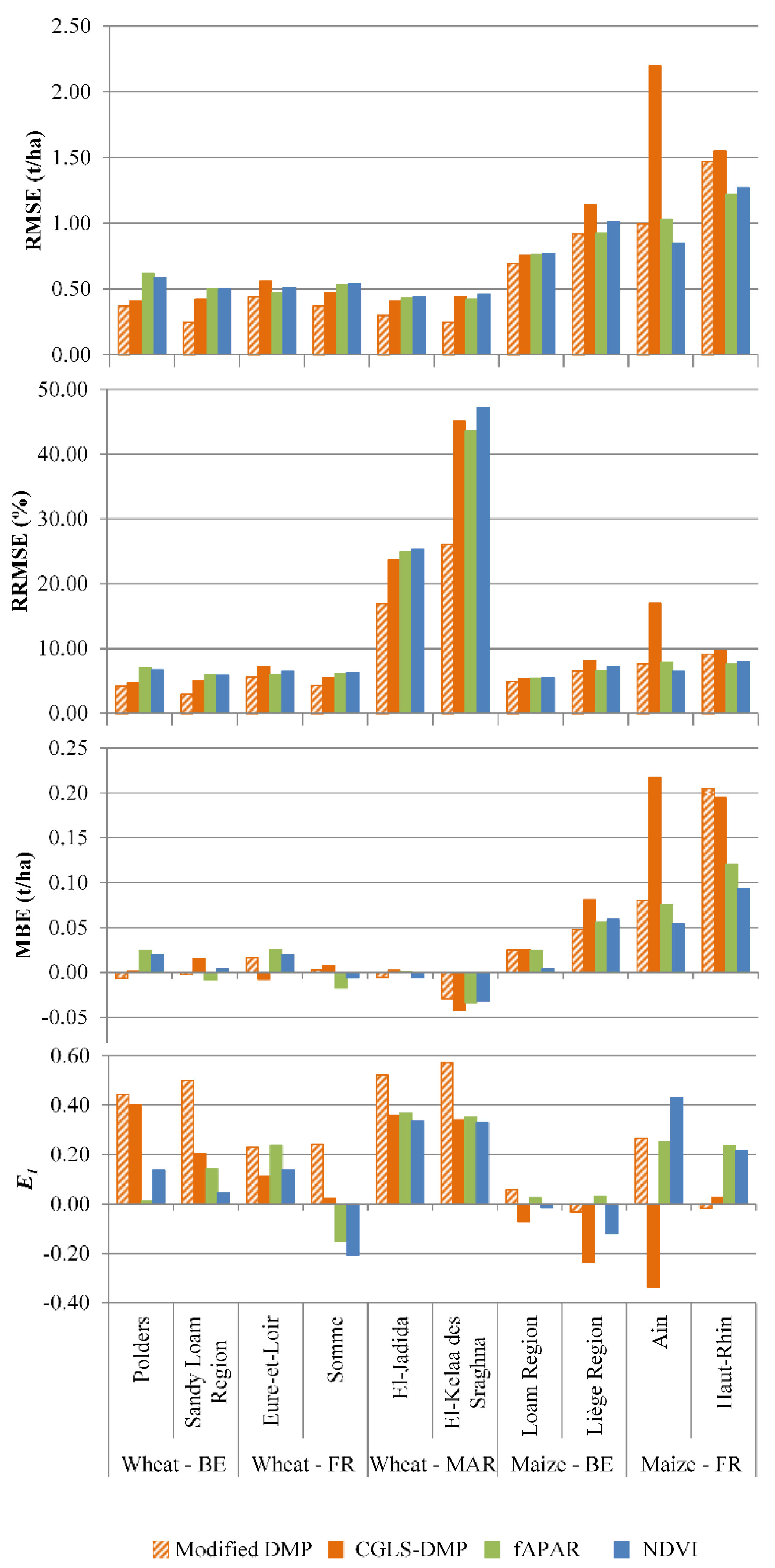
4.2. Linear Regression Analysis
5. Discussion
6. Conclusions
Supplementary Materials
Acknowledgments
Author Contributions
Conflicts of Interest
References
- Xin, Q.; Gong, P.; Yu, C.; Yu, L.; Broich, M.; Suyker, A.; Myneni, R. A production efficiency model-based method for satellite estimates of corn and soybean yields in the Midwestern US. Remote Sens. 2013, 5, 5926–5943. [Google Scholar] [CrossRef]
- Tao, F.; Yokozawa, M.; Zhang, Z.; Xu, Y.; Hayashi, Y. Remote sensing of crop production in China by production efficiency models: Models comparisons, estimates and uncertainties. Ecol. Model. 2005, 183, 385–396. [Google Scholar] [CrossRef]
- Wall, L.; Larocque, D.; Léger, P.M. The early explanatory power of NDVI in crop yield modelling. Int. J. Remote Sens. 2008, 29, 2211–2225. [Google Scholar] [CrossRef]
- Becker-Reshef, I.; Vermote, E.; Lindeman, M.; Justice, C. A generalized regression-based model for forecasting winter wheat yields in Kansas and Ukraine using MODIS data. Remote Sens. Environ. 2010, 114, 1312–1323. [Google Scholar] [CrossRef]
- Kogan, F.; Kussul, N.; Adamenko, T.; Skakun, S.; Kravchenko, O.; Kryvobok, O.; Shelestov, A.; Kolotii, A.; Kussul, O.; Lavrenyuk, A. Winter wheat yield forecasting in Ukraine based on earth observation, meteorological data and biophysical models. Int. J. Appl. Earth Obs. Geoinf. 2013, 23, 192–203. [Google Scholar] [CrossRef]
- López-Lozano, R.; Duveiller, G.; Seguini, L.; Meroni, M.; Garcia-Condado, S.; Hooker, J.D.; Leo, O.; Baruth, B. Towards regional grain yield forecasting with 1 km-resolution EO biophysical products: Strengths and limitations at pan-European level. Agric. For. Meteorol. 2015, 206, 12–32. [Google Scholar] [CrossRef]
- Doraiswamy, P.C.; Moulin, S.; Cook, P.W.; Stern, A. Crop yield assessment from remote sensing. Photogramm. Eng. Remote Sens. 2003, 69, 665–674. [Google Scholar] [CrossRef]
- Fensholt, R.; Sandholt, I.; Rasmussen, M.S. Evaluation of MODIS LAI, fAPAR and the relation between fAPAR and NDVI in a Semi-Arid environment using in situ measurements. Remote Sens. Environ. 2004, 91, 490–507. [Google Scholar] [CrossRef]
- Balaghi, R.; Tychon, B.; Eerens, H.; Jlibene, M. Empirical regression models using NDVI, rainfall and temperature data for the early prediction of wheat grain yields in Morocco. Int. J. Appl. Earth Obs. Geoinf. 2008, 10, 438–452. [Google Scholar] [CrossRef]
- Kuri, F.; Murwira, A.; Murwira, K.S.; Masocha, M. Predicting maize yield in Zimbabwe using dry dekads derived from remotely sensed vegetation condition index. Int. J. Appl. Earth Obs. Geoinf. 2014, 33, 39–46. [Google Scholar] [CrossRef]
- Prasad, A.K.; Chai, L.; Singh, R.P.; Kafatos, M. Crop yield estimation model for Iowa using remote sensing and surface parameters. Int. J. Appl. Earth Obs. Geoinf. 2006, 8, 26–33. [Google Scholar] [CrossRef]
- Gusso, A.; Ducati, J.R.; Veronez, M.R.; Arvor, D.; da Silveira, L.G. Spectral model for soybean yield estimate using. Int. J. Geosci. 2013, 2013, 1233–1241. [Google Scholar] [CrossRef]
- Meroni, M.; Marinho, E.; Sghaier, N.; Verstrate, M.; Leo, O. Remote sensing based yield estimation in a stochastic framework—Case study of durum wheat in Tunisia. Remote Sens. 2013, 5, 539–557. [Google Scholar] [CrossRef]
- Mkhabela, M.S.; Bullock, P.; Raj, S.; Wang, S.; Yang, Y. Crop yield forecasting on the Canadian prairies using MODIS NDVI Data. Agric. For. Meteorol. 2011, 151, 385–393. [Google Scholar] [CrossRef]
- Vicente-Serrano, S.; Cuadrat-Prats, J.; Romo, A. Early prediction of crop production using drought indices at different time scales and remote sensing data: Application in the Ebro Valley (North-East Spain). Int. J. Remote Sens. 2006, 27, 511–518. [Google Scholar] [CrossRef]
- Duveiller, G.; Baret, F.; Defourny, P. Remotely sensed green area index for winter wheat crop monitoring: 10-Year assessment at regional scale over a fragmented landscape. Agric. For. Meteorol. 2012, 166–167, 156–168. [Google Scholar] [CrossRef]
- Bastiaanssen, W.G.M.; Ali, S. A new crop yield forecasting model based on satellite measurements applied across the Indus basin, Pakistan. Agric. Ecosyst. Environ. 2003, 94, 321–340. [Google Scholar] [CrossRef]
- Liu, J.; Pattey, E.; Miller, J.R.; McNairn, H.; Smith, A.; Hu, B. Estimating crop stresses, aboveground dry biomass and yield of corn using multi-temporal optical data combined with a radiation use efficiency model. Remote Sens. Environ. 2010, 114, 1167–1177. [Google Scholar] [CrossRef]
- Pinker, R.T.; Zhao, M.; Wang, H.; Wood, E.F. Impact of satellite based PAR on estimates of terrestrial net primary productivity. Int. J. Remote Sens. 2010, 31, 5221–5237. [Google Scholar] [CrossRef]
- Swinnen, E.; van Hoolst, R.; Eerens, H. GIO-GL Lot 1, Algorithm Theoretical Basis Document, Dry Matter Productivity (DMP); EC Copernicus Global Land: Brussels, Belgium, 2015. [Google Scholar]
- Ajtay, G.L.; Ketner, P.; Duvigneaud, P. Terrestrial Primary Production and Phytomass; Bolin, B., Degens, E.T., Ketner, S., Kempe, P., Eds.; Wiley: New York, NY, USA, 1979. [Google Scholar]
- Garbulsky, M.F.; Peñuelas, J.; Papale, D.; Ardö, J.; Goulden, M.L.; Kiely, G.; Richardson, A.D.; Rotenberg, E.; Veenendaal, E.M.; Filella, I. Patterns and controls of the variability of radiation use efficiency and primary productivity across terrestrial ecosystems. Glob. Ecol. Biogeogr. 2010, 19, 253–267. [Google Scholar] [CrossRef]
- Ruimy, A.; Saugier, B.; Dedieu, G. Methodology for the estimation of terrestrial net primary production from remotely sensed data. J. Geophys. Res. 1994, 99, 5263. [Google Scholar] [CrossRef]
- Matsushita, B.; Xu, M.; Chen, J.; Kameyama, S.; Tamura, M. Estimation of regional Net Primary Productivity (NPP) using a process-based ecosystem model: How important is the accuracy of climate data? Ecol. Model. 2004, 178, 371–388. [Google Scholar] [CrossRef]
- Horn, J.E.; Schulz, K. Identification of a general light use efficiency model for gross primary production. Biogeosciences 2011, 8, 999–1021. [Google Scholar] [CrossRef]
- McCallum, I.; Wagner, W.; Schmullius, C.; Shvidenko, A.; Obersteiner, M.; Fritz, S.; Nilsson, S. Satellite-Based terrestrial production efficiency modeling. Carbon Balance Manag. 2009, 4. [Google Scholar] [CrossRef] [PubMed]
- Ruimy, A.; Kergoat, L.; Bondeau, A.; Intercomparison, T.P. Comparing global models of terrestrial Net Primary Productivity (NPP): Analysis of differences in light absorption and light use efficiency. Glob. Chang. Biol. 1999, 5, 56–65. [Google Scholar] [CrossRef]
- Monteith, J.L. Solar radiation and productivity in tropical ecosystems. J. Appl. Ecol. 1972, 9, 747. [Google Scholar] [CrossRef]
- Monteith, J.L.; Moss, C.J. Climate and the efficiency of crop production in britain [and discussion]. Philos. Trans. R. Soc. B Biol. Sci. 1977, 281, 277–294. [Google Scholar] [CrossRef]
- Sinclair, T.R.; Muchow, R.C. Radiation use efficiency. Adv. Agron. 1998, 65, 215–265. [Google Scholar]
- Field, C.B.; Randerson, J.T.; Malmström, C.M. Global net primary production: combining ecology and remote sensing. Remote Sens. Environ. 1995, 51, 74–88. [Google Scholar] [CrossRef]
- Goetz, S.J.; Prince, S.D.; Goward, S.N.; Thawley, M.M.; Small, J. Satellite remote sensing of primary production: An improved production efficiency modeling approach. Ecol. Model. 1999, 122, 239–255. [Google Scholar] [CrossRef]
- Running, S.W.; Thornton, P.E.; Nemani, R.R.; Glassy, J.M. Global Terrestrial gross and net primary productivity from the earth observing system. In Methods in Ecosystem Science; Sala, O., Jackson, R., Mooney, H., Eds.; Springer: New York, NY, USA, 2000; pp. 44–57. [Google Scholar]
- Xiao, X.; Hollinger, D.; Aber, J.; Goltz, M.; Davidson, E.A.; Zhang, Q.; Moore, B. Satellite-based modeling of gross primary production in an evergreen needleleaf forest. Remote Sens. Environ. 2004, 89, 519–534. [Google Scholar] [CrossRef]
- Potter, C.S.; Randerson, J.T.; Field, C.B.; Matson, P.A.; Vitousek, P.M.; Mooney, H.A.; Klooster, S.A. Terrestrial ecosystem production: A process model based on global satellite and surface data. Glob. Biogeochem. Cycles 1993, 7, 811–841. [Google Scholar] [CrossRef]
- Ruimy, A.; Dedieu, G.; Saugier, B. TURC: A diagnostic model of continental gross primary productivity and net primary productivity. Glob. Biogeochem. Cycles 1996, 10, 269–285. [Google Scholar] [CrossRef]
- Veroustraete, F.; Sabbe, H.; Eerens, H. Estimation of carbon mass fluxes over Europe using the C-Fix model and euroflux data. Remote Sens. Environ. 2002, 83, 376–399. [Google Scholar] [CrossRef]
- Running, S.W.; Nemani, R.R.; Heinsch, F.A.; Zhao, M.; Reeves, M.; Hashimoto, H. A Continuous Satellite-derived measure of global terrestrial primary production. Bioscience 2004, 54, 547–560. [Google Scholar] [CrossRef]
- Xiao, X.; Zhang, Q.; Braswell, B.; Urbanski, S.; Boles, S.; Wofsy, S.; Moore, B.; Ojima, D. Modeling gross primary production of temperate deciduous broadleaf forest using satellite images and climate data. Remote Sens. Environ. 2004, 91, 256–270. [Google Scholar] [CrossRef]
- Wu, C.; Niu, Z.; Gao, S. Gross primary production estimation from MODIS Data with vegetation index and photosynthetically active radiation in maize. J. Geophys. Res. Atmos. 2010, 115, 1–11. [Google Scholar] [CrossRef]
- Rossini, M.; Migliavacca, M.; Galvagno, M.; Meroni, M.; Cogliati, S.; Cremonese, E.; Fava, F.; Gitelson, A.; Julitta, T.; di Cella, U.M.; et al. Remote Estimation of grassland gross primary production during extreme meteorological seasons. Int. J. Appl. Earth Obs. Geoinf. 2014, 29, 1–10. [Google Scholar] [CrossRef]
- Ogutu, B.O.; Dash, J. Assessing the capacity of three production efficiency models in simulating gross carbon uptake across multiple biomes in conterminous USA. Agric. For. Meteorol. 2013, 174–175, 158–169. [Google Scholar] [CrossRef]
- Potter, C.; Klooster, S.; Tan, P.; Steinbach, M.; Kumar, V.; Genovese, V. Variability in terrestrial carbon sinks over two decades: Part 2—Eurasia. Glob. Planet. Chang. 2005, 49, 177–186. [Google Scholar] [CrossRef]
- Cao, M.; Prince, S.D.; Small, J.; Goetz, S.J. Remotely sensed interannual variations and trends in terrestrial net primary productivity 1981–2000. Ecosystems 2004, 7, 233–242. [Google Scholar] [CrossRef]
- Lafont, S.; Kergoat, L.; Erard, G.; Chevillard, A.; Karstens, U.; Kolle, O. Spatial and temporal variability of land CO2 Fluxes estimated with remote sensing and analysis data. Tellus 2002, 54B, 820–833. [Google Scholar] [CrossRef]
- Heinsch, F.A.; Zhao, M.; Running, S.W.; Kimball, J.S.; Nemani, R.R.; Davis, K.J.; Bolstad, P.V.; Cook, B.D.; Desai, A.R.; Ricciuto, D.M.; et al. Evaluation of remote sensing based terrestrial productivity from MODIS using regional tower eddy flux network observations. IEEE Trans. Geosci. Remote Sens. 2006, 44, 1908–1923. [Google Scholar] [CrossRef]
- Sasai, T.; Ichii, K.; Yamaguchi, Y.; Nemani, R. Simulating terrestrial carbon fluxes using the new biosphere model “biosphere model integrating Eco-physiological and Mechanistic approaches using satellite data” (BEAMS). J. Geophys. Res. 2005, 110, 1–18. [Google Scholar] [CrossRef]
- Verstraeten, W.W.; Veroustraete, F.; Feyen, J. On temperature and water limitation of net ecosystem productivity: Implementation in the C-Fix Model. Ecol. Model. 2006, 199, 4–22. [Google Scholar] [CrossRef]
- Wang, W.; Dungan, J.; Hashimoto, H.; Michaelis, A.R.; Milesi, C.; Ichii, K.; Nemani, R.R. Diagnosing and assessing uncertainties of terrestrial ecosystem models in a multimodel ensemble experiment: 1. Primary production. Glob. Chang. Biol. 2011, 17, 1350–1366. [Google Scholar] [CrossRef]
- Cramer, W.; Kicklighter, D.W.; Bondeau, A.; Moore, B.; Churkina, G.; Nemry, B.; Ruimy, A.; Schloss, A.L.; Intercompariso, N.P.P.M. Comparing global models of terrestrial Net Primary Productivity (NPP): Overview and key results. Glob. Chang. Biol. 1999, 5, 1–15. [Google Scholar] [CrossRef]
- Turner, D.P.; Ritts, W.D.; Cohen, W.B.; Maeirsperger, T.K.; Gower, S.T.; Kirschbaum, A.A.; Running, S.W.; Zhao, M.; Wofsy, S.C.; Dunn, A.L.; et al. Site-level evaluation of satellite-based global terrestrial gross primary production and net primary production monitoring. Glob. Chang. Biol. 2005, 11, 666–684. [Google Scholar] [CrossRef]
- Chirici, G.; Anna, B.; Maselli, F. Modelling of Italian forest net primary productivity by the integration of remotely sensed and GIS Data. For. Ecol. Manage. 2007, 246, 285–295. [Google Scholar] [CrossRef]
- Maselli, F.; Argenti, G.; Chiesi, M.; Angeli, L.; Papale, D. Simulation of grassland productivity by the combination of ground and satellite data. Agric. Ecosyst. Environ. 2013, 165, 163–172. [Google Scholar] [CrossRef]
- Chiesi, M.; Fibbi, L.; Genesio, L.; Gioli, B.; Magno, R.; Maselli, F.; Moriondo, M.; Vaccari, F.P. Integration of ground and satellite data to model Mediterranean forest Processes. Int. J. Appl. Earth Obs. Geoinf. 2011, 13, 504–515. [Google Scholar] [CrossRef]
- Veroustraete, F.; Patyn, J.; Myneni, R.B. Estimating net ecosystem exchange of carbon using the normalized difference vegetation index and an ecosystem model. Remote Sens. Environ. 1996, 58, 115–130. [Google Scholar] [CrossRef]
- Swinnen, E.; Van Hoolst, R.; Toté, C. GIO Global Land Component—Lot I “Operation of the Global Land Component”, Framework Service Contract N° 388533 (JRC), Quality Assessment Report, Dry Matter Productivity (DMP); EC Copernicus Global Land: Brussels, Belgium, 2014. [Google Scholar]
- Smets, B.; Swinnen, E.; Van Hoolst, R. GIO-GL Lot 1, Product User Manual, Dry Matter Productivity (DMP); EC Copernicus Global Land: Brussels, Belgium, 2015. [Google Scholar]
- Maselli, F.; Papale, D.; Puletti, N.; Chirici, G.; Corona, P. Combining remote sensing and ancillary data to monitor the gross productivity of water-limited forest ecosystems. Remote Sens. Environ. 2009, 113, 657–667. [Google Scholar] [CrossRef]
- Veroustraete, F.; Sabbe, H.; Rasse, D.P.; Bertels, L. Carbon mass fluxes of forests in Belgium determined with low resolution optical sensors. Int. J. Remote Sens. 2004, 25, 769–792. [Google Scholar] [CrossRef]
- Yuan, W.; Liu, S.; Yu, G.; Bonnefond, J.; Chen, J.; Davis, K.; Desai, A.R.; Goldstein, A.H.; Gianelle, D.; Rossi, F.; et al. Remote Sensing of environment global estimates of evapotranspiration and gross primary production based on MODIS and global meteorology data. Remote Sens. Environ. 2010, 114, 1416–1431. [Google Scholar] [CrossRef]
- Beer, C.; Reichstein, M.; Ciais, P.; Farquhar, G.D.; Papale, D. Mean annual GPP of Europe derived from its water balance. Geophys. Res. Lett. 2007, 34, L05401. [Google Scholar] [CrossRef]
- Amthor, J. The McCree–de Wit–Penning de Vries–Thornley respiration paradigms: 30 years later. Ann. Bot. 2000, 86, 1–20. [Google Scholar] [CrossRef]
- MARSOP-3. AGRI4CAST Interpolated Meteorological Data. Available online: http://mars.jrc.ec.europa.eu/mars/About-us/AGRI4CAST/Data-distribution/AGRI4CAST-Interpolated-Meteorological-Data (accessed on 18 May 2015).
- Westenbroek, S.M.; Kelson, V.A.; Dripps, W.R.; Hunt, R.J.; Bradbury, K.R. SWB—A Modified Thornthwaite-Mather Soil-Water- Balance Code for Estimating Groundwater Recharge: U.S. Geological Survey Techniques and Methods 6–A31; U.S. Geological Survey: Middleton, WI, USA, 2010.
- Gobin, A. Modelling climate impacts on crop yields in Belgium. Clim. Res. 2010, 44, 55–68. [Google Scholar] [CrossRef]
- Gobin, A. Impact of heat and drought stress on arable crop production in Belgium. Nat. Hazards Earth Syst. Sci. 2012, 12, 1911–1922. [Google Scholar] [CrossRef]
- Van der Velde, M.; Wriedt, G.; Bouraoui, F. Estimating irrigation use and effects on maize yield during the 2003 heatwave in France☆. Agric. Ecosyst. Environ. 2010, 135, 90–97. [Google Scholar] [CrossRef]
- Balaghi, R.; Jlibene, M.; Tychon, B.; Eerens, H. Agrometeorological Cereal Yield Forecasting in Morocco; INRA: Rabat, Morocco, 2013. [Google Scholar]
- VITO. Product Distribution Portal. Available online: http://www.vito-eodata.be/PDF/portal/Application.html#Home (accessed on 18 May 2015).
- ESA. GlobCover. Available online: http://due.esrin.esa.int/page_globcover.php (accessed on 18 May 2015).
- JRC. European Soil Database. Available online: http://eusoils.jrc.ec.europa.eu/ESDB_Archive/ESDB/index.htm (accessed on 18 May 2015).
- FAO. Digital Soil Map of the World. Available online: http://data.fao.org/map?entryId=446ed430-8383-11db-b9b2-000d939bc5d8 (accessed on 18 May 2015).
- FAO SDRN. AgroMetShell. Available online: http://www.hoefsloot.com/agrometshell.htm (accessed on 18 May 2015).
- Yildiz, H.; Mermer, A.; Aydogdu, M. Forecasting of winter wheat yield for turkey using water balance model. In Proceedings of the Fourth International Conference on Agro-Geoinformatics, Istanbul, Turkey, 20–24 July 2015; pp. 352–356.
- NTSG. MODIS NPP/GPP Project. Available online: http://www.ntsg.umt.edu/project/mod17 (accessed on 11 August 2015).
- Gobron, N.; Pinty, B.; Aussedat, O.; Chen, J.M.; Cohen, W.B.; Fensholt, R.; Gond, V.; Huemmrich, K.F.; Lavergne, T.; Mélin, F.; et al. Evaluation of fraction of absorbed photosynthetically active radiation products for different canopy radiation transfer regimes: Methodology and results using joint research center products derived from SeaWiFS against ground-based estimations. J. Geophys. Res. 2006, 111, D13110. [Google Scholar] [CrossRef]
- Wang, K. Acclimation of photosynthetic parameters in scots pine after three years exposure to elevated temperature and CO2. Agric. For. Meteorol. 1996, 82, 195–217. [Google Scholar] [CrossRef]
- Kang, E.; Lu, L.; Xu, Z. Vegetation and carbon sequestration and their relation to water resources in an inland river basin of Northwest China. J. Environ. Manage. 2007, 85, 702–710. [Google Scholar] [CrossRef] [PubMed]
- Atwell, B.J.; Kriedemann, P.E.; Turnbull, C.G. Plants in Action: Adaptation in Nature, Performance in Cultivation; Macmillan Education Australia: Melbourne, Australia, 1999. [Google Scholar]
- Bonhomme, R. Bases and limits to using “Degree day” Units. Eur. J. Agron. 2000, 13, 1–10. [Google Scholar] [CrossRef]
- Brown, D.; Bootsma, A. Crop heat units for corn and other warm season crops in Ontario. In Factsheet Ministry of Agriculture and Food Ontario; OMAFRA: Guelph, ON, Canada, 1993; pp. 1–6. [Google Scholar]
- Warrington, I.J.; Kanemasu, E.T. Corn growth response to temperature and photoperiod I. Seedling emergence, tassel initiation, and anthesis. Agron. J. 1983, 75, 749–754. [Google Scholar] [CrossRef]
- Warrington, I.J.; Kanemasu, E.T. Corn growth response to temperature and photoperiod II. Leaf-initiation and leaf- appearance rates. Agron. J. 1983, 75, 755–761. [Google Scholar] [CrossRef]
- White, J.W. Modeling temperature response in wheat and maize. In Proceedings of the Workshop, CIMMYT, El Bata´n, Mexico, 23–25 April 2001.
- Yan, W.; Hunt, L.A. An equation for modelling the temperature response of plants using only the cardinal temperatures. Ann. Bot. 1999, 84, 607–614. [Google Scholar] [CrossRef]
- Tollenaar, M.; Mihajlovic, M.; Aguilera, A. Temperature response of dry matter accumulation, leaf photosynthesis, and chlorophyll fluorescence in an old and a new maize hybrid during early development. Can. J. Plant Sci. 1991, 71, 353–359. [Google Scholar] [CrossRef]
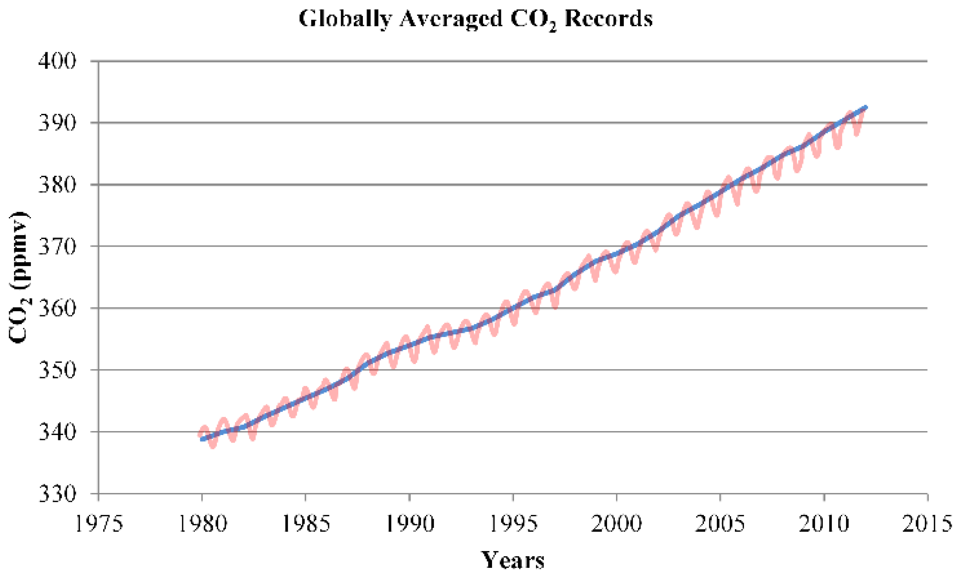
- NOAA. CO2 Records. Available online: http://www.esrl.noaa.gov/gmd/ccgg/trends (accessed on 20 October 2015).
- Ainsworth, E.A.; Long, S.P. What have we learned from 15 years of Free-Air CO2 Enrichment (FACE)? A meta-analytic review of the responses of photosynthesis, canopy properties and plant production to rising CO2. New Phytol. 2005, 165, 351–372. [Google Scholar] [CrossRef] [PubMed]
- Wang, C.; Guo, L.; Li, Y.; Wang, Z. Systematic comparison of C3 and C4 plants based on metabolic network analysis. BMC Syst. Biol. 2012, 6, S9. [Google Scholar] [CrossRef] [PubMed]
- Yin, X.; Struik, P.C. C3 and C4 Photosynthesis models: An overview from the perspective of crop modelling. NJAS—Wageningen J. Life Sci. 2009, 57, 27–38. [Google Scholar] [CrossRef]
- Kim, S.; Gitz, D.; Sicher, R.; Baker, J.; Timlin, D.; Reddy, V. Temperature dependence of growth, development, and photosynthesis in maize under elevated CO2. Environ. Exp. Bot. 2007, 61, 224–236. [Google Scholar] [CrossRef]
- Von Caemmerer, S. Biochemical Models of Leaf Photosynthesis; CSIRO: Collingwood, Australia, 2000. [Google Scholar]
- Goetz, S.J.; Prince, S.D.; Goward, S.N.; Thawley, M.M.; Small, J.; Johnston, A. Mapping net primary production and related biophysical variables with remote sensing: Application to the BOREAS region. J. Geophys. Res. 1999, 104, 27719. [Google Scholar] [CrossRef]
- Prince, S.D.; Goward, S.N. Global primary production: A remote sensing approach. J. Biogeogr. 1995, 22, 815–835. [Google Scholar] [CrossRef]
- Dabrowska-Zielinska, K.; Kowalik, W.; Budzynska, M.; Malek, I. Assessment of Evapotranspiration and Soil Moisture for Biebrza Wetlands Using Thermal Remote Sensing and In-Situ Data; Halounová, L., Ed.; EARSel: Prague, Czech Republic, 2011; pp. 281–288. [Google Scholar]
- Duveiller, G.; López-Lozano, R.; Baruth, B. Enhanced processing of 1-km spatial resolution fAPAR time series for sugarcane yield forecasting and monitoring. Remote Sens. 2013, 5, 1091–1116. [Google Scholar] [CrossRef]
- Legates, D.R.; Mccabe, G.J. A refined index of model performance: A rejoinder. Int. J. Climatol. 2013, 33, 1053–1056. [Google Scholar] [CrossRef]
- Zhang, Y.; Xu, M.; Chen, H.; Adams, J. Global pattern of NPP to GPP ratio derived from MODIS Data: Effects of ecosystem type, geographical location and climate. Glob. Ecol. Biogeogr. 2009, 18, 280–290. [Google Scholar] [CrossRef]
- Salazar, L.; Kogan, F.; Roytman, L. Use of remote sensing data for estimation of winter wheat yield in the United States. Int. J. Remote Sens. 2007, 28, 3795–3811. [Google Scholar] [CrossRef]
- Mkhabela, M.S.; Mkhabela, M.S.; Mashinini, N.N. Early maize yield forecasting in the four agro-ecological regions of Swaziland Using NDVI Data Derived from NOAA’s-AVHRR. Agric. For. Meteorol. 2005, 129, 1–9. [Google Scholar] [CrossRef]
- Funk, C.; Budde, M.E. Phenologically-tuned MODIS NDVI-based production anomaly estimates for Zimbabwe. Remote Sens. Environ. 2009, 113, 115–125. [Google Scholar] [CrossRef]
- Ren, J.; Chen, Z.; Zhou, Q.; Tang, H. Regional yield estimation for winter wheat with MODIS-NDVI Data in Shandong, China. Int. J. Appl. Earth Obs. Geoinf. 2008, 10, 403–413. [Google Scholar] [CrossRef]
- Sakamoto, T.; Gitelson, A.A.; Arkebauer, T.J. MODIS-based corn grain yield estimation model incorporating crop phenology information. Remote Sens. Environ. 2013, 131, 215–231. [Google Scholar] [CrossRef]
- Hansen, J.W.; Indeje, M. Linking dynamic seasonal climate forecasts with crop simulation for maize yield prediction in Semi-Arid Kenya. Agric. For. Meteorol. 2004, 125, 143–157. [Google Scholar] [CrossRef]
- Klein, A. Bulletin Agro-Météorologique: Ajustement Des Dates de Semis; Université de Liège: Arlon, Belgium, 2014. [Google Scholar]
- LSA SAF. Evapotranspiration. Available online: http://landsaf.meteo.pt/algorithms.jsp?seltab=7&starttab=7 (accessed on 11 August 2015).
- Hu, G.; Jia, L.; Menenti, M. Comparison of MOD16 and LSA-SAF MSG evapotranspiration products over Europe for 2011. Remote Sens. Environ. 2015, 156, 510–526. [Google Scholar] [CrossRef]
- Ise, T.; Moorcroft, P.R. Simulating boreal forest dynamics from perspectives of ecophysiology, resource availability, and Climate Change. Ecol. Res. 2010, 25, 501–511. [Google Scholar] [CrossRef]
- Procter, A.C. Effects of Past and Future CO2 on Grassland Soil Carbon and Microbial Ecology; Duke University: Durham, NC, USA, 2012. [Google Scholar]
- Polley, H.W.; Derner, J.D.; Jackson, R.B.; Wilsey, B.J.; Fay, P.A. Impacts of climate change drivers on C4 grassland productivity: Scaling driver effects through the plant community. J. Exp. Bot. 2014, 65, 3415–3424. [Google Scholar] [CrossRef] [PubMed]
- Waraich, E.A.; Ahmad, R.; Halim, A.; Aziz, T. Alleviation of temperature stress by nutrient management in crop plants: A review. J. Soil Sci. Plant Nutr. 2012, 12, 221–244. [Google Scholar] [CrossRef]
- Gitelson, A.A.; Peng, Y.; Masek, J.G.; Rundquist, D.C.; Verma, S.; Suyker, A.; Baker, J.M.; Hatfield, J.L.; Meyers, T. Remote estimation of crop gross primary production with landsat data. Remote Sens. Environ. 2012, 121, 404–414. [Google Scholar] [CrossRef]
- Gitelson, A.A.; Viña, A.; Masek, J.G.; Verma, S.B.; Suyker, A.E. Synoptic monitoring of gross primary productivity of maize using Landsat data. IEEE Geosci. Remote Sens. Lett. 2008, 5, 133–137. [Google Scholar] [CrossRef]
- Peng, Y.; Gitelson, A.A. Application of chlorophyll-related vegetation indices for remote estimation of maize productivity. Agric. For. Meteorol. 2011, 151, 1267–1276. [Google Scholar] [CrossRef]
- Phillips, L.; Hansen, A.; Flather, C. Evaluating the species energy relationship with the newest measures of ecosystem energy: NDVI versus MODIS primary production. Remote Sens. Environ. 2008, 112, 4381–4392. [Google Scholar] [CrossRef]
- EPA. Climate Impacts on Agriculture and Food Supply. Available online: http://www.epa.gov/climatechange/impacts-adaptation/agriculture.html (accessed on 10 February 2015).
- Deryng, D.; Conway, D.; Ramankutty, N.; Price, J.; Warren, R. Global crop yield response to extreme heat stress under multiple climate change futures. Environ. Res. Lett. 2014, 9, 034011. [Google Scholar] [CrossRef]
- Luterbacher, J.; Dietrich, D.; Xoplaki, E.; Grosjean, M.; Wanner, H. European seasonal and annual temperature variability, trends, and extremes since 1500. Science 2004, 303, 1499–1503. [Google Scholar] [CrossRef] [PubMed]
- Duveiller, G.; Lopez-Lozano, R.; Cescatti, A. Exploiting the multi-angularity of the MODIS temporal signal to identify spatially homogeneous vegetation cover: A demonstration for agricultural monitoring applications. Remote Sens. Environ. 2015, 166, 61–77. [Google Scholar] [CrossRef]
- Baruth, B.; Kucera, L. Crop masking—Needs for the mars crop yield forecasting system. In Proceedings of the ISPRS XXXVI-8/W48 Workshop: Remote Sensing Support to Crop Yield Forecast and Area Estimates, Stresa, Italy, 30 November–1 December 2006; pp. 3–6.


| Soil Type | Soil Texture | |||
|---|---|---|---|---|
| Wheat | BE | Polders | Calcaric Regosols + Calcaric Fluvisols | Loam + Silt loam |
| Sandy Loam Region | Dystric Podzoluvisols + Orthic Luvisols | Sandy loam + Loam | ||
| FR | Eure-et-Loir | Gleyic Luvisols + Orthic Luvisols | Clay Loam + Loam | |
| Somme | Orthic Luvisols | Loam | ||
| MAR | El Jadida | Calcic Kastanozems + Vertisols + Eutric Fluvisols | Loam + Silty Clay + Silt Loam | |
| El Kelaa | Eutric Gleysols + Calcic Xerosols | Clay Loam + Loam | ||
| Maize | BE | Loam Region | Orthic Luvisol + Dystric Podzoluvisol | Loam + Sandy Loam |
| Liège Region | Stagno-Gleyic Luvisol + Orthic Luvisols + Dystric Cambisol | Clay Loam + Loam + Silt Loam | ||
| FR | Ain | Gleyic Luvisols + Orthic Luvisols + Eutric Cambisols | Clay Loam + Loam + Silt Loam | |
| Haut Rhin | Gleyic Luvisols + Orthic Luvisols | Clay Loam + Loam |
| January | February | March | April | May | June | July | August | September | October | November | December | ||||||||||||||
|---|---|---|---|---|---|---|---|---|---|---|---|---|---|---|---|---|---|---|---|---|---|---|---|---|---|
| Wheat | BE | Polders | |||||||||||||||||||||||
| Sandy Loam Region | |||||||||||||||||||||||||
| FR | Eure-et-Loir | ||||||||||||||||||||||||
| Somme | |||||||||||||||||||||||||
| MAR | El-Jadida | ||||||||||||||||||||||||
| El-Kelaa des Sraghna | |||||||||||||||||||||||||
| Maize | BE | Loam Region | |||||||||||||||||||||||
| Liège Region | |||||||||||||||||||||||||
| FR | Ain | ||||||||||||||||||||||||
| Haut-Rhin | |||||||||||||||||||||||||
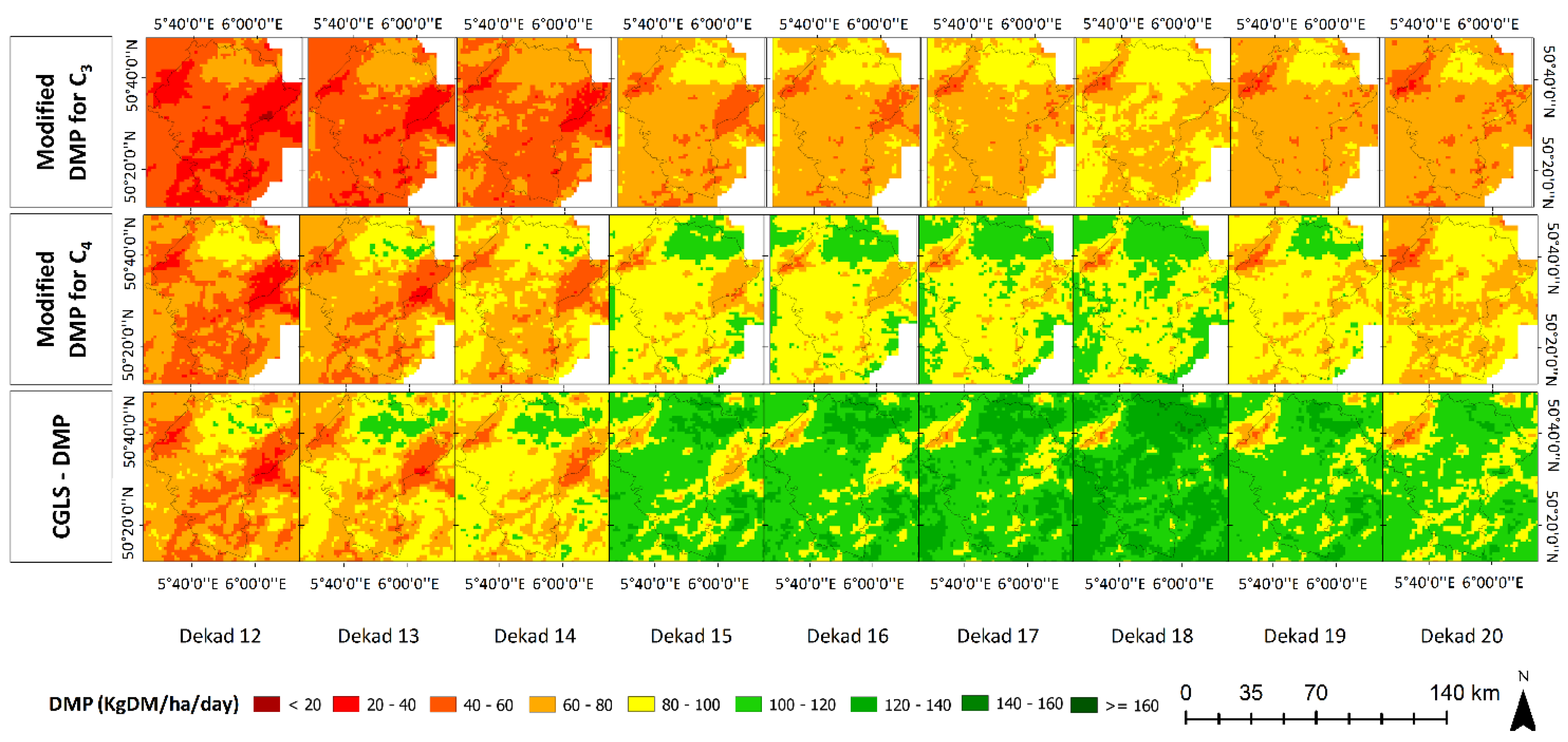
| CGLS-DMP | Modified DMP | ||
|---|---|---|---|
| Obtained from JRC-MARSOP on a daily basis at a 0.25° grid | |||
| Derived from 10-daily SPOT VGT imagery at 1km² resolution | |||
| No water stress factor | Water stress factor based on AET | ||
| C3 plants (wheat) | C4 plants (maize) | ||
| 2.54 kgDM/GJ for all C3 plants | 2.75 kgDM/GJ for wheat | 3.5 kgDM/GJ for maize | |
| Blue curve in Figure 3 | Blue curve in Figure 3 | Red curve in Figure 3 | |
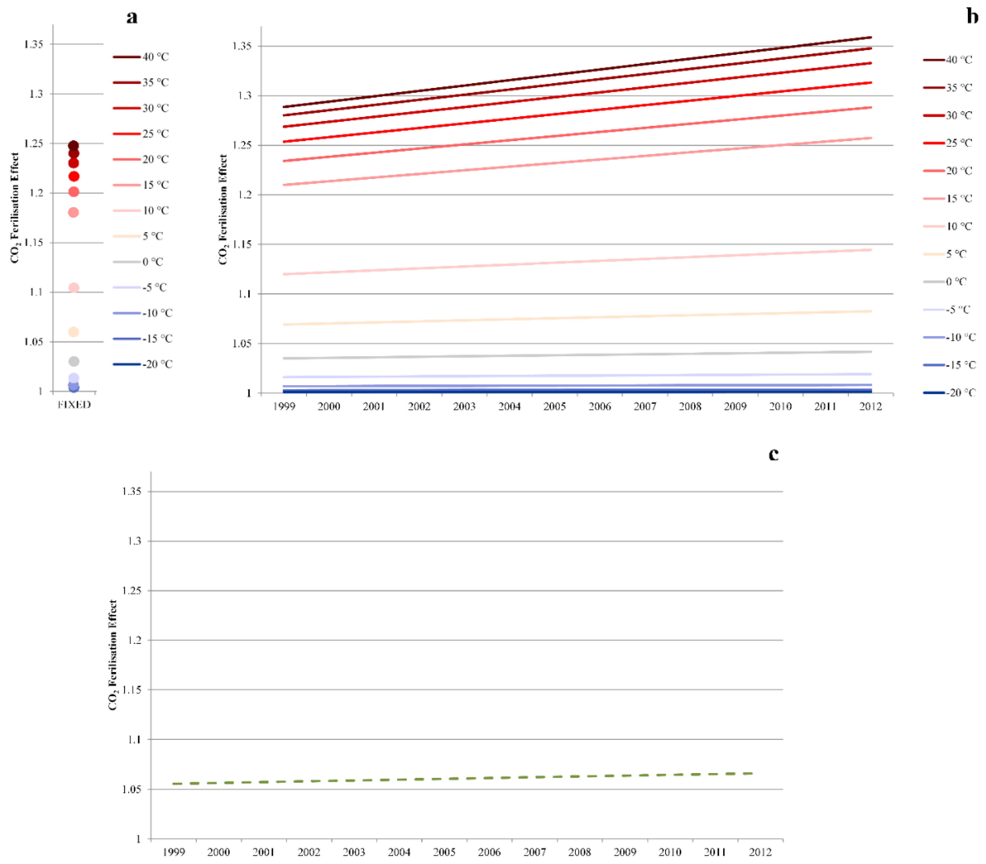
| Blue to red dots in Figure 5a | Blue to red lines in Figure 5b | Dashed green line in Figure 5c | |
| Figure 7a, range: 0.65–0.85 for study regions | Figure 7b, range: 0.5–0.7 for study regions | ||
© 2016 by the authors; licensee MDPI, Basel, Switzerland. This article is an open access article distributed under the terms and conditions of the Creative Commons by Attribution (CC-BY) license (http://creativecommons.org/licenses/by/4.0/).
Share and Cite
Durgun, Y.Ö.; Gobin, A.; Gilliams, S.; Duveiller, G.; Tychon, B. Testing the Contribution of Stress Factors to Improve Wheat and Maize Yield Estimations Derived from Remotely-Sensed Dry Matter Productivity. Remote Sens. 2016, 8, 170. https://doi.org/10.3390/rs8030170
Durgun YÖ, Gobin A, Gilliams S, Duveiller G, Tychon B. Testing the Contribution of Stress Factors to Improve Wheat and Maize Yield Estimations Derived from Remotely-Sensed Dry Matter Productivity. Remote Sensing. 2016; 8(3):170. https://doi.org/10.3390/rs8030170
Chicago/Turabian StyleDurgun, Yetkin Özüm, Anne Gobin, Sven Gilliams, Grégory Duveiller, and Bernard Tychon. 2016. "Testing the Contribution of Stress Factors to Improve Wheat and Maize Yield Estimations Derived from Remotely-Sensed Dry Matter Productivity" Remote Sensing 8, no. 3: 170. https://doi.org/10.3390/rs8030170
APA StyleDurgun, Y. Ö., Gobin, A., Gilliams, S., Duveiller, G., & Tychon, B. (2016). Testing the Contribution of Stress Factors to Improve Wheat and Maize Yield Estimations Derived from Remotely-Sensed Dry Matter Productivity. Remote Sensing, 8(3), 170. https://doi.org/10.3390/rs8030170