Grassland and Cropland Net Ecosystem Production of the U.S. Great Plains: Regression Tree Model Development and Comparative Analysis

Abstract

This paper presents the methodology and results of two ecological-based net ecosystem production (NEP) regression tree models capable of up scaling measurements made at various flux tower sites throughout the U.S. Great Plains. Separate grassland and cropland NEP regression tree models were trained using various remote sensing data and other biogeophysical data, along with 15 flux towers contributing to the grassland model and 15 flux towers for the cropland model. The models yielded weekly mean daily grassland and cropland NEP maps of the U.S. Great Plains at 250 m resolution for 2000–2008. The grassland and cropland NEP maps were spatially summarized and statistically compared. The results of this study indicate that grassland and cropland ecosystems generally performed as weak net carbon (C) sinks, absorbing more C from the atmosphere than they released from 2000 to 2008. Grasslands demonstrated higher carbon sink potential (139 g C·m⁻²·year⁻¹) than non-irrigated croplands. A closer look into the weekly time series reveals the C fluctuation through time and space for each land cover type.

1. Introduction

The far reaching effects and evidence of climate change, driven by increases in atmospheric greenhouse gas concentrations, motivated international mitigation focus at the 2015 United Nations Framework Convention on Climate Change Fifteenth Session of the Conference of the Parties [1]. Regional syntheses of carbon flux tower data [2,3,4] provide geographically referenced estimates from multiple flux towers and offer detailed summarization of carbon flux properties.

Throughout modern history, scientists have been developing models to formulate generalized algorithms to expand geographically and temporally sparse field observations to a much larger landscape means [2,3,4] or to make up-scaled maps of the measured field characteristics [5]. Understanding, mapping, and quantifying regional carbon flux magnitudes and variability of terrestrial non-point carbon sinks (removal of atmospheric carbon) and sources (emission of carbon to the atmosphere) is important in the promotion of ecosystem sustainability. Methodological and technological advances in the areas of remote sensing, environmental monitoring devices, data management, and computer-aided analytics have led the way to more innovative modeling. With these advancements, scientists have been able to apply these modeling methods to make estimates about discrete environmental characteristics, such as, atmospheric composition and below ground characteristics [6,7,8,9].

Remote sensing data [5,10,11], light use efficiency modeling [9,12], data mining techniques [5,10,11,13,14], process-base modeling [15,16], and greenhouse gas inventories [17] have enhanced regional understanding and monitoring capabilities. Mapping efforts are sometimes at coarse resolutions, long time step intervals, have large (continental or global) study areas which may miss local detail, and can have highly automated or general gap filling strategies for temporary flux tower instrument failures.

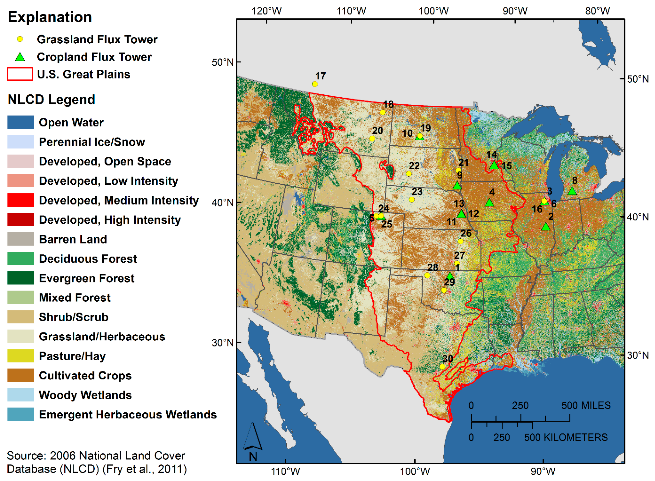
Our analysis focused on two primary large ecosystem classes in the U.S. Great Plains, cropland and grassland. We developed and applied our models at the 250 m spatial resolution and the weekly temporal resolution to retain the detailed temporal dynamics of carbon fluxes in the output maps. The primary objective of this study was to combine measurements acquired at flux towers with applicable remote sensing, weather, and other biogeophysical data to develop separate grassland and cropland ecologically-based net ecosystem production (NEP) models and derive mean daily NEP maps at a weekly time step from 2000 to 2008 for the study area of interest, the U.S. Great Plains (Figure 1). Although a flux tower measures only its surrounding vicinity, numerous studies have shown that these recordings can be used in regional or land cover specific synthesis [3,4] or up-scaled to much greater levels through analyses of geospatial data relationships using computer modeling [9,13,18]. Of particular interest is the use of data mining regression tree algorithms for carbon flux mapping [5,10,11,13,14,18]. 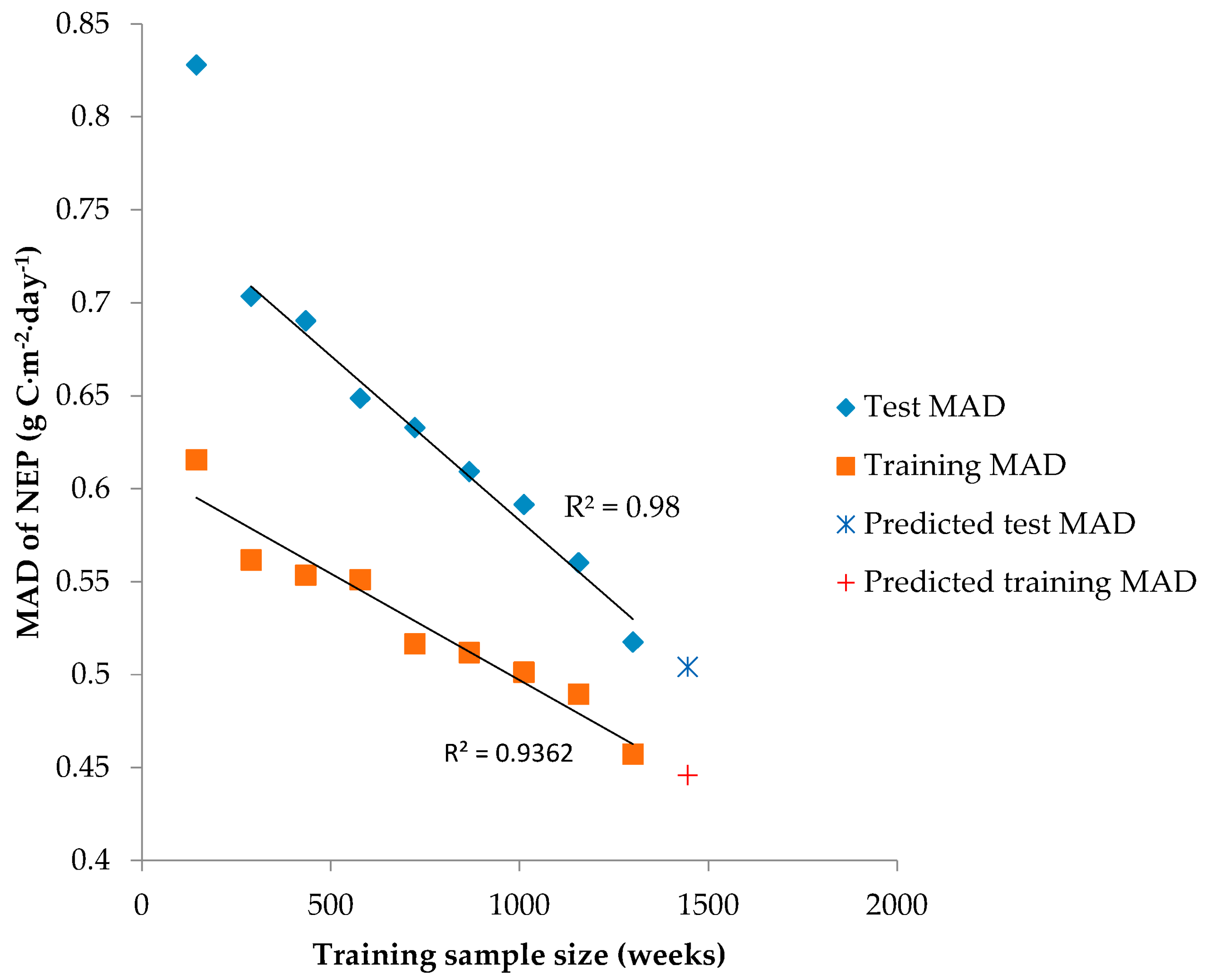An acute capability to address nonlinear relationships, deal with complex high order interactions, easily interpret results, and utilize both categorical and continuous variables, lends data mining regression tree [10], which contrasts with process-based modeling approaches that are frequently heavily driven by precipitation, a difficult variable to map accurately, particularly in rural regions where weather stations are sparse. A vulnerability of regression tree approaches is a tendency of over fitting. However, this can be mitigated through cross validation [19] and generalization of sequential dichotomous tests (trees) into generalized rules [20]. Regional comparisons indicated a higher grassland carbon sink strength and a higher water use efficiency than non-irrigated crops across rainfall gradients in the Great Plains.

In addition to model development and map production, a secondary objective of this study was to perform a systematic comparative analysis of the grassland and cropland NEP results. Our hypothesis was that cropland ecosystems, being highly managed to optimize productivity of usually annual vegetation and often in a state of tilled (exposed) soil, vulnerable to respiration losses, would lean more towards the C sources. Conversely, grasslands with perennial vegetation, generally subject to little management and no tillage, would tend to perform as C equilibrium or sinks. Grassland and cropland make up approximately 85% of the total surface area of the U.S. Great Plains (48% grasslands or shrubs and 37% cultivated crops, pasture, or hay; Figure 1), signifying the importance of understanding C fluxes in these two ecosystem classes. This spatial and temporal synthesis of Ameriflux, Agriflux, and independent flux tower data was performed with attention to the stated goals of the North American Carbon Program (NACP) [22].

2. Materials and Methods

2.1. Flux Tower Data

Dynamics of carbon dioxide (CO₂) exchange and other ecosystem resource characteristics are being measured by flux towers at observation sites throughout the world. For short stature vegetation (crops, shrubs, and grasses), the flux tower fetch area is about 250 m. NEP flux data sets were at the 30 min time scale and subsequently aggregated to daily and weekly time steps. A flux tower utilizes systems, such as eddy covariance and Bowen Ratio methods, to continuously measure the exchanges of CO₂, water vapor, and energy between terrestrial ecosystems and the atmosphere [23]. Globally, there are over 500 active flux towers currently operating on a long-term and continual basis. These flux towers are located in a diverse range of land cover types, such as, forests, croplands, grasslands, shrublands, wetlands, and tundra. For this study, flux tower data sets from sites located in grassland and cropland within or near the Great Plains and during the 2000–2008 time frame were identified, acquired, and processed (Table S1). We used NEP at the 30 min time step from the flux towers to quality control for possible instrument related outliers. The quality controlled carbon flux data sets were partitioned into gross primary production (GPP) and ecosystem respiration (Re) components utilizing light response and vapor pressure-based partitioning of carbon flux into GPP and Re components [2,3,4]. Partitioning the fluxes into GPP and Re facilitated a more functional filling of temporary flux tower data gaps [24]. Partitioned and gap-filled GPP and Re and NEP used in this mapping effort were largely from focused regional flux tower synthesis for grain crops [4], leguminous crops [3], and grasslands [2]. We selected the carbon flux light response and vapor pressure, or “non-rectangular hyperbolic method” flux partitioning models [2,3,4] over Q₁₀ and short-term exponential fit models (which model Re as a function of temperature based on night-time data) and rectangular hyperbolic fit models (which use the relationship between photosynthetic active radiation (PAR) and daytime NEP to model Re) because it produces the most reasonable C flux estimates and data gap filling [25], particularly in non-forest, low canopy height systems. NEP data from the flux towers were summarized into weekly periods aligning with 7-day expedited Moderate Resolution Imaging Spectroradiometer (eMODIS) Normalized Difference Degetation Index (NDVI) composites [26]. The training of the grassland and cropland NEP mapping models for weekly NEP was focused on records from 30 flux towers—15 measuring CO₂ exchange (CFlux) in cropland sites and 15 measuring CFlux in grassland sites (Figure 1, Table S1). The 30 flux towers represent a total of 76 site years of data (33 site years for grassland and 43 site years for cropland).

2.2. Input Spatial Data

To bring the flux tower data into proper context and permit upscaling to the U.S. Great Plains, a wide range of input spatial data were selected and implemented in the regression tree model training (Section 2.4 below). Model development and mapping application at the weekly time step of NEP helped capture seasonal variations of NEP that are related to both weather and management activities. These input data sets provided the models with samples of how NEP behaves in accordance with variability of various spatial and temporal environmental characteristics. The first group of input spatial data used in model training included weekly eMODIS NDVI [26] and a simple temporal dataset with values ranging from 1 to 52 for the week of the year. NDVI is derived from visible and near-infrared (NIR) light reflectance measurements (Equation (1)) and correlates with the photosynthetic potential of vegetation [27]. The eMODIS NDVI product [26] is processed using the same data source and atmospheric correction algorithms as the standard MODIS collection 5 data product [28]. However, the eMODIS process uses a compositing algorithm which is largely dependent on maximum value-NDVI compositing, scan angle, and data quality flags to filter through input reflectance with bad quality, negative values, clouds, snow cover, or low view angles. Additional eMODIS NDVI quality measures were performed to reduce possible cloud contamination and anomalous atmospheric effects by applying temporal smoothing using a moving window weighted least-squares regression method [29]. While NDVI is a widely accepted vegetation index (VI) that has numerous applications [11,14,30], some disadvantages have been noted, such as spectral signature saturation in areas of high canopy density [31]. The weekly NDVI and temporal datasets were used to train the models on how NEP corresponds to weekly vegetation vigor.

$$\mathrm{NDVI}=\frac{\mathrm{NIR}-\mathrm{red}}{\mathrm{NIR}+\mathrm{red}}$$

(1)

The second set of spatial input data was selected to allow the models to capture how NEP responds to weekly meteorological-based characteristics. These included weekly total precipitation (PCP), weekly mean minimum and maximum air temperature (TMIN and TMAX), and weekly mean PAR acquired from the National Weather Service (NWS) National Centers for Environmental Prediction (NCEP) [32]; 30-year normals for annual TMIN, TMAX, mean temperature (TMEAN), and PCP for the 1981 to 2010 time period were also incorporated into the model. These normals were acquired from the PRISM Climate Group [33] and rescaled from 800 m to 250 m using bi-linear interpolation.

The third set of input spatial data used in model training included several annual vegetation phenology metrics to train the models on how NEP fluctuates as a function of varying seasonality and states of vegetation. Specifically, nine unique annual phenology metrics, derived using methodology in accordance with Reed, et al. [34], were incorporated into the models. The phenology metrics included Amplitude (AMP), Duration (DUR), End of Season NDVI (EOSN), End of Season Time (EOST), Maximum NDVI (MAXN), Maximum NDVI Time (MAXT), Start of Season NDVI (SOSN), Start of Season Time (SOST), and Time Integrated NDVI (TIN). All phenology metrics were acquired from the U.S. Geological Survey (USGS) Remote Sensing Phenology (RSP) website [35].

The fourth group of input spatial data used in model training included four static soil variables, derived from the Soil Survey Geographic (SSURGO) database (mostly mapped at the 1:24,000 scale), where available, with gaps filled from the State Soil Geographic (STATSGO) database. These soil datasets were acquired from the U.S. Department of Agriculture (USDA), Natural Resources Conservation Service (NRCS) [36]. The four soil variables were available water capacity (AWC), clay percentage (CP), bulk density (BD), and soil organic carbon (SOC) within a 0–30 cm soil depth zone. This set of static inputs was included to train the models on how NEP varies as a function of soil characteristics.

Finally, the models were referenced to a specific land cover or vegetation type. For the grassland NEP model, the land cover type was all grassland and the weekly grass NEP from Zhang, et al. [11] was used. The cropland NEP model added annual crop information. These data were acquired from the crop type maps (CTM) developed by Howard and Wylie [37]. Only crops for which flux tower data were available were included (corn, soybeans, wheat, and alfalfa). General land cover/land use datasets, such as, ecoregion (ECO) [38], major land resource areas (MLRA) [39], and irrigation in 2002, 2007, and 2012 (IRR) [40] were also used in constructing the model.

Table 1. Input spatial datasets used in the development of the grassland and cropland NEP models.

Source Type	Derived Dataset	Acronym	NEP Model Application	Temporal Interval
MODIS	Normalized Difference Vegetation Index	NDVI	Grassland and Cropland	Weekly
Meteorological Characteristics	Total Precipitation	PCP	Grassland and Cropland	Weekly
Meteorological Characteristics	Mean Minimum Air Temperature	TMIN	Grassland and Cropland	Weekly
Meteorological Characteristics	Mean Maximum Air Temperature	TMAX	Grassland and Cropland	Weekly
Meteorological Characteristics	Mean Photosynthetic Active Radiation	PAR	Grassland Only	Weekly
Temporal Variable	Week/Day of Year	Week/DOY	Grassland and Cropland	Weekly
MODIS-Based Phenology	Amplitude	AMP	Cropland Only	Annual
MODIS-Based Phenology	Duration	DUR	Cropland Only	Annual
MODIS-Based Phenology	End of Season NDVI	EOSN	Cropland Only	Annual
MODIS-Based Phenology	End of Season Time	EOST	Cropland Only	Annual
MODIS-Based Phenology	Maximum NDVI	MAXN	Grassland and Cropland	Annual
MODIS-Based Phenology	Maximum NDVI Time	MAXT	Grassland and Cropland	Annual
MODIS-Based Phenology	Start of Season NDVI	SOSN	Grassland and Cropland	Annual
MODIS-Based Phenology	Start of Season Time	SOST	Grassland and Cropland	Annual
MODIS-Based Phenology	Time Integrated NDVI	TIN	Grassland and Cropland	Annual
NRCS SSURGO	Percent clay in soil	CLAY	Cropland	Static
MODIS-Based Crop Classifications	Crop Type	CTM	Cropland Only	Annual
30-year Normals	Annual Precipitation	C_PPT	Cropland Only	Static
30-year Normals	Annual Mean Maximum Air Temperature	C_TMAX	Cropland Only	Static
30-year Normals	Annual Mean Air Temperature	C_TMEAN	Cropland Only	Static
30-year Normals	Annual Mean Minimum Air Temperature	C_TMIN	Cropland Only	Static
SSURGO/STATSGO-Based Soil Properties	Available Water Capacity (0–30 cm soil depth)	AWC	Grassland and Cropland	Static
NRCS SSURGO	Percent clay (0–30 cm)	CLAY	Cropland	Static
SSURGO/STATSGO-Based Soil Properties	Clay Percentage (0–30 cm soil depth)	CP	Cropland Only	Static
SSURGO/STATSGO-Based Soil Properties	Bulk Density (0–30 cm soil depth)	BD	Cropland Only	Static
SSURGO/STATSGO-Based Soil Properties	Soil Organic Carbon (0–30 cm soil depth)	SOC	Cropland Only	Static
Land Use/Cover Classification	Level 3 Ecoregion	ECO	Grassland and Cropland	Static
Land Use/Cover Classification	Major Land Resource Areas	MLRA	Cropland Only	Static
Land Use/Cover Classification	Irrigation	IRR	Cropland Only	Static

gives a complete list of the input spatial data utilized in the training of grassland and cropland NEP regression tree models.

2.3. Data Standardization

All source input spatial data were put through a series of data standardization procedures to ensure spatial and temporal consistencies. Common geoprocessing techniques were employed to resample and spatially align the input data to an Albers equal-area conic projection with a 250 m pixel size and masked to the U.S. Great Plains boundary. Spatial inputs with a temporal element, such as the meteorological data (generated from daily composites), were appropriately aggregated to match the weekly time intervals of the eMODIS NDVI composite periods. Finally, model application masks were developed according to the target land cover of each NEP model (cropland or grassland) based on NLCD classifications. The cropland mask was defined based on “Cultivated Crops” and “Pasture/Hay” and the grassland mask was defined based on “Grassland/Herbaceous” and “Pasture/Hay”. “Pasture/Hay” was included in the cropland mask because there was a potential of alfalfa falling into this class. This masking configuration introduced an overlap between the two NEP mapping results and was handled by averaging the two in the overlapping areas [41].

2.4. Regression Tree Model Development

The two regression tree mapping models in this study were developed using Cubist software [41] based on the methodology as described by Zhang, et al. [11]. Cubist was used because of its use of generalized rules and widespread successful applications in the remote sensing field [5,10,11,14,18,42,43,44,45,46,47,48,49,50,51]. Each regression tree model consisted of the dependent variable to be estimated and the set of independent variables. The dependent variable in this case was the weekly NEP (grams (g) of C·m⁻²·week⁻¹) from the study flux towers (Table S1). A potential drawback to regression tree models is a tendency of overfitting (substantial differences between test and training accuracy). These overfitting tendencies were assessed and minimized through nine model training iterations with varying data set sizes. Each training data set size was replicated nine times with different random seeds.

Analysis of the GNU General Public License of Cubist [41] revealed that the ruleset (stratification for piecewise regressions and regression independent variable selection) cost function is the mean absolute difference modified by the ratio of the number of cases and the number of parameters. This weights the process towards having fewer parameters and trying to simplify the model as a whole while countering against over fitting and mitigating outlier impacts. More classical least squares approaches tend to be more sensitive to outliers than to absolute difference. The multiple regression determination for each ruleset is a classical least squares approach excluding extreme residual outliers.

The models were designed to ingest a series of input spatial data and estimate the weekly mean daily cropland and grassland NEP throughout the U.S. Great Plains for 2000 to 2008 at 250 m spatial resolution. Under the ecological-based notation, NEP is defined as subtracting RE from GPP and denotes the net exchange of carbon between terrestrial ecosystems and the atmosphere where the ecosystem is the point of reference (Equation (2)). Therefore, any ecosystem that absorbs more carbon (C) than it releases would yield a positive NEP value and would be considered a C sink. Conversely, any ecosystem that releases more C than it absorbs would yield a negative NEP value and would be considered a C source.

$$\mathrm{NEP}=\left(\mathrm{GPP}-\mathrm{RE}\right),$$

(2)

The model training process (Figure S1) begins by first spatially and temporally linking the flux tower data with the spatial datasets to create the training database for each model. To achieve this, the flux tower data were converted into point shapefiles with the accompanying weekly NEP records. Next, these points where spatially and temporally intersected with each of the input spatial datasets to extract the full set of input values at each point. Through this procedure, the flux tower point and accompanying NEP records were merged with the appropriate input spatial dataset values, creating the final training databases. The training data base used for developing the cropland NEP regression tree model contained 2225 samples of weekly NEP acquired from 15 flux tower locations over 13 years with temporal coverage varying by flux tower. Likewise, the grassland NEP regression tree model was trained on 1447 weekly samples acquired from 15 flux tower locations over 9 years.

These data bases were then ingested into RuleQuest Cubist v. 2.06 data mining software [41] to construct the regression tree mapping models (Figure S1). Cubist ingests the training data bases, analyzes them for patterns and relationships between the independent and the dependent variables, and uses this information to create models consisting of numerous estimation rules in the form of multiple ‘if-then-else’ conditional statements. The completed models are in turn implemented on a pixel-by-pixel basis to estimate NEP, the dependent variable, based on the set of input spatial data, outputting a weekly map.

The validation and accuracy assessment of the Cubist regression tree NEP mapping models quantified model training accuracy and model spatial and temporal accuracy through a series of leave-one-out cross validation techniques. The cross validation method withholds a specific group of flux data (data from a particular flux tower, year, or a random sample of weekly fluxes) from model development as an independent test and the mapping model is developed from the remaining flux dataset. The cross validation approach is widely accepted [52,53,54,55] and has been used in C flux mapping [5,10,11,13,18] and biomass mapping [47,56], as well as to assess expected model performance on unseen data, identify of influential flux towers and years, and to help optimize models to minimize over fitting (using random cross validation) [19,57,58]. Cross validation approaches provide robust accuracy assessments from many independent withheld “test” data, which helps to identify and minimize over fitting or over generalization [59], and allows all of the limited flux towers to be utilized in developing the final mapping models—maximizing mapping accuracy and robustness for crop and grassland NEP.

Our experience with Cubist models for mapping has indicated the potential for a substantial variation of test accuracies with different randomizations of test data or different sites or years being withheld as test [11,51]. Cross validation techniques allow multiple independent test data sets to estimate the expected accuracies of the population of pixels to be mapped and can better quantify accuracy variability across multiple random test datasets than the classical single independent data test dataset approach. To further quantify the robustness of our flux mapping algorithms, we utilized an approach similar to the “bias/variance tradeoff” approach [59]. With this approach, the input variables and the maximum allowed number of committee sub-models are held constant while the various size combinations of test and training are assessed [60]. The training data size (or proportion of the total weekly flux tower observations) in this experiment was increased in 10% increments from 10% to 90% with the test datasets decreasing inversely from 90% to 10%. At each level of training dataset size, we performed nine different random seeds for test data selections (nine training dataset sizes with nine different randomizations = 81 model runs). Across the nine randomizations at each level of training dataset size, the mean absolute difference (MAD) was calculated to quantify training and test accuracies, the standard deviation of MAD quantified model stability for training and test datasets at each level of training dataset size, and the MAD difference between test and training datasets quantified model over fitting. Relationships between test accuracy and training accuracies were established as a function of training dataset size to extrapolate expected model tendencies when trained on 100% of the flux tower data (which was used for map generation).

Under sampling by reference or training data relative to the space and time to be mapped is an issue in both machine learning approaches and process-based mapping models used to map carbon fluxes [5,9,51,61], but the area to be mapped to number of flux tower ratios were similar in this study to other carbon flux mapping efforts [5,13,18].

2.5. NEP Map Production

The grassland and cropland NEP regression tree models were applied to the U.S. Great Plains using the input spatial data applicable to each model and time period to produce weekly NEP maps. For example, the cropland model was implemented for week 1 of 2000 by using all week 1 data from 2000 (NDVI, Week, PCP, TMIN, and TMAX), all annual data from 2000 (AMP, DUR, EOSN, EOST, MAXN, MAXT, SOSN, SOST, TIN, and CTM), along with the static input datasets (30-year normal data, AWC, CP, BD, and SOC). In this example, the cropland model would yield the week 1 NEP cropland estimates for 2000. Through this model implementation process, 936 weekly, 250 m NEP maps for grassland and cropland of the U.S. Great Plains for 2000–2008 were produced (468 grassland NEP maps and 468 cropland NEP maps). Following the initial map development, a masking step was performed to remove areas where the dominant crop, during the 2000–2008 time period, was something other than corn, soybeans, winter wheat, or alfalfa (Figure S2).

2.6. Grass versus Crop NEP Comparison

Rangeland (grass) biomass strata or “classes” were derived from STATSGO estimates for a “normal year” from STATSGO estimates of rangeland production on a “normal” year [62] using an unsupervised clustering approach. Eight rangeland biomass strata were produced that captured the productivity and precipitation gradients of the central and western portions of the Great Plains (Figure 2). STATSGO rangeland biomass estimates were not available for the states east of this extent.

To assess normality (a requirement for the application of classical statistics) in regional NEP distributions several approaches were applied: visual inspection of NEP regional frequency plots and the differences between mean and median regional NEP indicated skewness. These normality assessments were applied to annual NEP, 2000–2008 combined NEP, and other spatial subsets (grass and specific crop types and eight rangeland productivity strata (classes) which captured productivity gradients across the Great Plains. Where non-normal NEP regional or sub-regional frequency distributions (crop, grass, productivity classes) were observed, we used median, MAD, and quartiles, otherwise classical statistics were applied (means and Root Means Square Error (RMSE)).

Mean and median annual NEP maps were derived from the 2000–2008 weekly grassland and cropland NEP regression tree output maps and were studied to gain an understanding of how Cflux corresponds to the Great Plains moisture and productivity gradients and potentially reveal conditions where grassland or cropland had greater carbon sink strength. This effort focused only on grass and non-irrigated cropland, as determined by Brown and Pervez [63], to exclude the substantial production advantages that come with irrigation.

The 2000–2008 mean and median NEP for grass and non-irrigated cropland was averaged across eight rangeland production classes derived from unsupervised clusters using STATSGO rangeland production estimates. Then, the eight rangeland productivity class median NEP for grasslands was regressed on median NEP for non-irrigated croplands. The intercept term from this relationship tested the significance (p < 0.05) of potential grass NEP differences when non-irrigated crops are at the 2000–2008 equilibrium. The slope coefficient will reveal potential variations of grass and non-irrigated crop NEP across the Great Plains production and moisture gradients. Similarly, 30-year gridded climate data [33] precipitation was averaged for each of the productivity classes and regressed on production class median grassland NEP and on production class median non-irrigated crop NEP. The intercept coefficients quantify precipitation levels where grass and non-irrigated crops can be expected to be in near 2000–2008 equilibrium. A similar analysis using biomass from each of the production classes can identify expected rangeland productivity levels where grass and non-irrigated crops would be near 2000–2008 equilibrium.

3. Results

3.1. Regression Tree Model

Model training accuracies for the crop and grass weekly NEP mapping algorithms are summarized in

Table 2. Summary of prediction accuracies of NEP (g C·m⁻²·day⁻¹) from model development (training), site cross validation, year cross validation, and a random test hypothetical projection.

	Intercept	Slope	p	r	RMSE	MAD
Croplands
Training	0.018	0.018 b	<0.01	0.94	1.01	0.60
Site cross validation	−0.098	0.675 b	<0.01	0.76	1.62	1.14
Year cross validation	0.127 a	1.101 b	<0.01	0.8	1.79	1.02
Hypothetical random test	na	na	na	na	na	0.71
Grassland
Training	−0.042 a	1.180 b	<0.0001	0.88	0.62	0.45
Site cross validation	0.033	0.339 b	<0.0001	0.48	1.14	0.81
Year cross validation	0.226 a	0.389 b	<0.0001	0.49	1.16	0.81
Hypothetical random test	na	na	na	na	na	0.53

^a Significantly different from 0; ^b significantly different from 1; na, Not applicable.

. The cropland NEP model training accuracy achieved a correlation coefficient (r) of 0.94, a RMSE of 1.01 g C·m⁻²·day⁻¹ a MAD of 0.60 g C·m⁻²·day⁻¹. The grass model training accuracy had an r of 0.88, RMSE of 0.62 g C·m⁻²·day⁻¹, and a MAD of 0.45 g C·m⁻²·day⁻¹. Given the large datasets (sample sizes of 1445–2277) used to develop the grass and crop regression trees. Autocorrelation effects are expected to be minor because the ordinary least squares estimators associated with the regression models are consistent under general conditions [64] and provide unbiased estimates [65]. The NEP regression tree mapping models for crops and grass are presented in Tables S2 and S3. All map legends and statistics were conformed to a common unit and are presented as NEP as g C·m⁻²·day⁻¹ or g C·m⁻²·year⁻¹.

The regression tree mapping rules and prediction regressions are completely transparent and quantify the multiple sequential models (committee models) from which a mean prediction is made. The crop model had 3 committee models that had between 17 and 21 different prediction strata or rules, while the grass model had 5 committee models with 10 to 31 different rules (Tables S2 and S3). Each rule has stratification criteria (“conditions”) as well as an associated multiple regression model (“prediction”), which is applied within a respective rule’s strata. The usage of independent variables in the model development data base with the respective multiple regression models are for deriving the model “predictions”. The number of weekly NEP flux tower observations in the model development data base that meet each rule’s stratification criteria is quantified (the number of weekly NEP flux tower observations or cases in Tables S2 and S3), and the percentage utilization of the spatial data inputs for stratification (“conditions”) can be quantified for each regression tree mapping model (see Attribute usage “condition”, or “model” at the end of Tables S2 and S3). An overall utilization for each spatial input was estimated by the mean utilization across attribute condition and use in the regression model (

Table 3. Utilization in percentage of the total weekly NEP fluxes for the spatial inputs used in mapping crop NEP.

Spatial Inputs	Attribute Conditions	Prediction	Mean Utilization
NDVI	81%	83%	82%
Week	78%	0%	39%
SOSN	10%	65%	38%
SOST	2%	73%	38%
AMP	4%	70%	37%
MAXN	0%	69%	35%
TMIN	15%	51%	33%
EOST	1%	61%	31%
DEM	0%	62%	31%
TMAX	4%	52%	28%
DUR	0%	54%	27%
TIN	4%	47%	26%
EOSN	2%	48%	25%
BD	6%	40%	23%
PCP	0%	41%	21%
MAXT	0%	40%	20%
SLP	0%	38%	19%
AWS	0%	36%	18%
C_PPT	0%	34%	17%
SOC	2%	24%	13%
CLAY	7%	17%	12%
C_TMAX	12%	10%	11%
Crop Type	21%	0%	11%
C_TMIN	0%	18%	9%
MLRA	8%	0%	4%
C_TMEAN	0%	5%	3%

and

Table 4. Utilization in percentage of the total weekly NEP fluxes for the spatial inputs used in mapping grass NEP.

Spatial Inputs	Attribute Conditions	Prediction	Mean Utilization
PAR	76%	60%	68%
NDVI	50%	44%	47%
DOY	46%	47%	47%
PPT	8%	57%	33%
MAXN	19%	45%	32%
AWS	28%	35%	32%
TIN	21%	39%	30%
SOSN	10%	45%	28%
TMIN	3%	45%	24%
TMAX	5%	40%	23%
MAXT	12%	31%	22%
SOST	12%	17%	15%

). The weekly eMODIS NDVI (proxy for photosynthetic potential of vegetation) was the most utilized spatial input variable in the crop model and PAR (primarily driven by day length and cloud cover) was the most utilized spatial variable in the grass model (Table S5). Time of year variables (Week in crop model and Day of Year (DOY) in grass model) were either the second or third most utilized spatial variables in both mapping models. Phenological variables (SOSN, SOST, AMP, MAXN, TMIN, and EOST) were much more important in the crop model (Table S4) than in the grass model and maybe implying that crop fluxes are more closely tied to phenology than grass or that crop phenological metrics are more accurately mapped from NDVI time series than grasslands. Precipitation was more influential in the grass model than in the crop model largely because precipitation was not used in the stratification of the crop model and it may be related to the higher probability of irrigation in croplands than in grasslands. AWC was the most important soil characteristic (better than SOC, BD, and CLAY) and was much more important in the grass model than in the crop model (32 versus 18 percent, respectively).

3.2. Validation

Leave one site out cross validation was conducted to assess crop and grass flux prediction consistency on unseen data and also to identify influential flux towers (

Table 5. Leave-one-out flux tower site cross validation for crops and grasslands (g C·m⁻²·day⁻¹).

Site	Site ID	Mean of Flux Tower	Std. Dev. of Flux Tower	Mean of Estimated	Std. Dev. of Estimated	RMSE	MAD	Influence Rank
Cropland
Lamont ARM Main	1	0.11	1.73	−0.33	2.63	2.58	1.71	1
Bondville	2	na	na	na	na	na	na
Batavia	3	na	na	na	na	na	na
Brooks Field-10	4	0.15	2.85	0.22	2.73	1.81	1.00	6
Curtis Ranch	5	−0.03	0.64	−0.80	0.90	1.41	1.00	7
Fermi Agricultural	6	na	na	na	na	na	na
Haller	7	na	na	na	na	na	na
Kellogg Biological Station	8	na	na	na	na	na	na
Lennox	9	0.41	2.95	0.59	2.93	1.21	0.85	9
Mandan	10	0.69	2.00	0.13	1.36	1.79	1.39	2
Mead Irrigated Continuous	11	0.37	3.66	0.16	2.43	1.73	1.01	5
Mead Rainfed	12	1.13	4.51	0.61	2.97	2.46	1.22	3
Mead Irrigated Rotation	13	−0.08	1.99	−0.15	2.12	1.07	0.70	10
Rosemount Conventional	14	0.42	2.98	0.41	2.03	1.62	1.00	8
Rosemount G19	15	0.19	1.97	−0.21	1.13	1.95	1.14	4
Mean						1.76	1.10
Grassland
Batavia	16	0.7	2.33	na	na	na	na
Lethbridge	17	0.3	1.36	na	na	na	na
Fort Peck	18	−0.21	1.12	0.26	1.05	1.61	1.08	1
Mandan	19	0.25	0.89	0.1	0.74	1.06	0.77	7
Miles City	20	−0.21	0.77	−0.51	0.41	0.9	0.67	13
Brookings	21	0.08	1.3	0.36	0.97	1.2	0.9	4
Cottonwood	22	−0.08	0.91	0.14	0.97	0.98	0.62	9
Gudmundsen Ranch	23	−0.07	0.99	−0.04	0.44	0.92	0.7	12
CPER	24	0.18	1.13	0.33	0.68	0.96	0.7	10
CRP ungrazed	25	−0.43	0.81	−0.45	0.57	0.94	0.7	11
Rannells Ranch	26	0.45	1.88	0.17	0.88	1.47	1	2
Walnut River	27	0.14	1.15	0.01	0.76	0.99	0.73	8
Woodward	28	0.24	1.15	0.01	1.12	1.1	0.89	6
Fort Reno	29	0.16	1.63	0.62	1.08	1.14	0.91	5
Freeman Ranch	30	0.14	0.93	−0.9	0.78	1.35	1.09	3
Mean						1.12	0.83

na, Not applicable (flux tower outside the Great Plains).

). Leave one site out cross validation is a pessimistic error estimation particularly for influential flux towers. The crop mean MAD was 1.10 g C·m⁻²·day⁻¹, and ranged from 0.70 to 1.71 g C·m⁻²·day⁻¹. The most influential flux tower was Lamont ARM Main which represents a low yield dryland cropping system; this tower was the southern-most crop site, and one of two winter wheat sites. Mandan was the second most influential flux tower, which may be related to the crop type with Mandan being one of only two alfalfa flux towers. Additional cropland flux towers located in poorly represented crops would improve model confidence and robustness. Flux-tower known weekly NEP was regressed on predicted weekly NEP when each respective flux tower location was withheld as a test in the cross validation by site analysis. An overall, highly significant (p < 0.01) regression model had an coefficient of determinations (R²) of 0.57, an RMSE of 1.62 g C·m⁻²·day⁻¹, and a MAD of 1.14 g C·m⁻²·day⁻¹ (Table 2)—which was quite similar to the table means of the leave-one-out flux tower site (Table 5). Similar NEP mapping accuracies were reported by [13] but, at a global scale, it had a much coarser spatial resolution (0.5 degree) and a longer mapping time step.

The grassland leave one site out cross validation (also shown in Table 5) analysis indicated slightly lower NEP error terms than the cropland model with a mean RMSE of 1.12 g C·m⁻²·day⁻¹ (ranging from 0.9 to 1.61 g C·m⁻²·day⁻¹); and a mean MAD of 0.83 g C·m⁻²·day⁻¹ (ranging from 0.62 to 1.09 g C·m⁻²·day⁻¹). Fort Peck was the most influential grassland flux tower because it captured an extreme drought year (2002). Rannells Ranch was the second most influential flux tower of the grassland model. An overall regression of withheld weekly grassland NEP had similar error magnitudes (Table 2) as the leave one site cross validation means (Table 5). The lower NEP error terms that were observed for grass relative to crops persisted in the weekly regression of withheld grass predictions with a RMSE of 1.14 g C·m⁻²·day⁻¹ and a MAD of 0.81 g C·m⁻²·day⁻¹ (Table 2). These lower grass leave-one-out cross validation error terms may be related to the diverse crop types (the monoculture nature of crop stands resulted in abrupt vegetation differences) and the intensive management of crops. Grassland communities are typically more diverse mixtures of forbs and C₃ and C₄ grasses, often have gradual transitions in species compositions, and management impacts are not as intensive as croplands.

Leave-one-out cross validation quantified the robustness of mapping models through time (

Table 6. Year leave-one-out cross validation of weekly NEP (g C·m⁻²·day⁻¹).

Year	Mean of Flux Tower	Std. Dev. of Flux Tower	Mean of Estimated	Std. Dev. of Estimated	r	RMSE	MAD	Influence Rank
Cropland
2000	−0.22	2.45	1.19	3.43	0.93	2.02	1.42	3
2001	1.08	4.13	0.26	2.64	0.85	2.50	1.43	1
2002	0.20	2.85	0.27	2.40	0.86	1.44	1.00	7
2003	0.75	3.85	0.64	2.47	0.82	2.32	1.36	2
2004	0.08	2.29	0.08	1.62	0.83	1.32	0.79	9
2005	0.46	2.63	0.13	1.40	0.82	1.72	0.96	6
2006	0.29	2.56	−0.05	1.48	0.74	1.81	0.99	5
2007	0.48	3.18	0.22	2.43	0.81	1.91	1.06	4
2008	0.09	2.22	0.03	1.95	0.78	1.40	0.79	8
Mean					0.83	1.82	1.09
Grassland
2000	0.12	1.19	0.34	0.93	0.61	0.99	0.68	6
2001	0.13	0.96	0.08	0.79	0.63	0.77	0.54	8
2002	0.07	1.29	0.38	0.96	0.15	1.52	1.03	1
2003	0.25	1.38	−0.06	0.77	0.48	1.25	0.92	3
2004	0.04	1.05	0.79	1.20	0.55	1.31	0.95	2
2005	0.26	1.53	0.31	1.04	0.65	1.17	0.88	5
2006	0.04	1.30	0.44	1.15	0.59	1.18	0.88	4
2007	−0.22	0.93	0.04	0.92	0.50	0.96	0.70	7
2008	na	na	na	na	na	na	na
Mean					0.52	1.14	0.82

na, Not applicable (no flux tower used from 2008).

). The cropland mean RMSE and the mean MAD from the leave-one-year-out analysis had similar magnitudes as the leave-one-site-out analysis. Interestingly, we see 2001 was the most influential year—the year the Lamont winter wheat flux tower recorded very low crop yields. Similarly, the leave-one-year-out cross validation had similar across-year mean RMSE and MAD as the leave-one-out site across site mean values. This demonstrates a consistency in the crop and grass NEP mapping models for both cross validation techniques (through time and space). The most influential year in the grass NEP model was 2002, a drought year [66].

The robustness and over fitting tendencies for the cropland flux mapping regression tree models documented higher randomized test MAD for the crop model than the training MAD at all levels of training data size (over fitting), but over fitting tendencies (difference between training and test MAD) declined to acceptable levels (<0.20 g C·m⁻²·day⁻¹) with low MAD test and training differences [7,10] with larger training data sizes (Figure 3). Training MAD was relatively constant across the training data size variations, which indicates an increase in the cropland NEP mapping model robustness to unseen data with increasing training data size. Crop NEP MAD regressed on training data size (R² = 0.82) estimated a hypothetical training MAD of 0.71 g C·m⁻²·day⁻¹ when all the flux tower data were used as training.

The grassland NEP models demonstrated that smaller random test sizes had larger error components (MAD) for both model training and testing (Figure 4). This was especially true of the lowest training sample size’s associated test MAD, which also had a MAD standard deviation nearly double the other test MAD estimates. This result indicated an unstable model at this low training sample size and was considered an outlier. The continuing decline of both the test and training MAD for the grassland NEP mapping model would imply that additional flux tower observations would continue to improve both the accuracy and robustness of the mapping model. The test MAD declined dramatically with increasing training size (R² = 0.98) indicating a rapid decrease in over fitting tendencies. The test MAD regression (excluding the outlier test MAD at the low training sample size) estimated a hypothetical test MAD of 0.50 g C·m⁻²·day⁻¹ when all the grass weekly NEP observations were used in model development.

3.3. NEP Maps

The NEP maps were combined into merged cropland and grassland products and summarized to quantify NEP in the U.S. Great Plains at weekly, seasonal, and annual time steps. Specifically, four groups of maps were produced from the merged weekly grassland and cropland NEP maps: (1) mean weekly NEP; (2) annual NEP; (3) mean seasonal NEP; and (4) mean annual NEP. Each of these maps represented the cumulative NEP (in g C·m⁻² specified time·period⁻¹) using ecological-based notation [3,10,11], where negative values indicate areas with higher RE than GPP (C source) and positive values indicate areas with higher GPP than RE (C sink). The annual maps (Figure 5) showed the level of variability of cumulative NEP from one year to the next [67], while the mean seasonal (Figure 6) and weekly NEP maps captured the intra-annual dynamics of NEP. The mean annual 2000–2008 map (Figure 7) proved useful in identifying the prevalent NEP condition during 2000–2008.

To quantify the spatial variation of multiple year NEP uncertainty, a regression tree model was developed to estimate leave one site out cross validation accuracies from vegetation type (crop or grass), soil organic carbon, 30-year mean annual precipitation, and mean annual NEP. This three member committee Cubist model (two rules for each committee model) predicted the leave-one-out site RMSE with a training MAD of 0.18 g C·m⁻²·day⁻¹ (r = 0.91) and a random 10-fold cross validation MAD of 0.22 g C·m⁻²·day⁻¹ (r = 0.87). The similarity between the training and cross validation MADs implies minimal over fitting tendencies. The resultant RMSE map (Figure 8) was masked by crop and grassland areas and stratified (see legend) by the percentage the three input variables exceeded the data values observed at the flux tower locations (extrapolation index). RMSE tends to be higher in cropland areas and lower in grassland areas similar to the results shown in Table 5, but also reflects grassland domination in drier western portions of the Great Plains. Also, western agriculture is often dominated by irrigation, which results in higher production, NEP, and RMSE.

These maps present an important NEP archive of a large portion of the U.S. Great Plains for the 2000–2008 time period and, when coupled with the following statistical analysis quantifying and comparing NEP behavior in the U.S. Great Plains, could be utilized for various carbon-cycle-based analyses.

3.4. Comparisons between Grassland and Cropland across the Great Plains

Crop and grass NEP across the Great Plains indicated drops in grassland NEP in 2002 and 2006, which where years with high incidences of drought [69], particularly in July [66], in western grassland areas. The yearly overlap of the 25th and 75th quartiles for grass and crops is substantial resulting in the multiple year medians for crops and grass being quite similar (Figure 9).

Crop type differences in median Great Plains NEP show that carbon sink potential is the greatest with alfalfa and corn (Figure 10). The 25% quartiles of alfalfa exceed the 75% quartile of grass in 2004, 2005, 2007, and 2008, indicating minimal overlap. Similarly, the corn 25% quartiles exceed the 75% quartile of grass in 2002 and 2006, both major drought years.

More detailed, weekly-iterated statistics revealed even greater detail about the annual dynamics of NEP in grassland and cropland ecosystems (Figure 6 and Figure 11, and Table S4). Both ecosystems averaged out to have minor C source tendencies during the winter weeks when vegetation is typically in a dormant state and GPP and RE are minimal. Grassland generally exhibited the earlier increase and peak to NEP in the spring, which is likely related to perennial C3 grasses and forbs. Conversely, cropland maintained higher RE rates than GPP throughout the spring, a time when fields are being prepared, seeds planted, and initial emergence takes place. In the summer, grasslands tended to level off and start on a decreasing NEP trend throughout the remainder of the year, while cropland GPP spikes and increases to a maximum NEP in mid-summer. Around harvest time, in the fall, cropland generally declined to C source levels similar to those observed in the spring.

3.5. Great Plains Productivity Gradient Comparisons between Grassland and Non-Irrigated Cropland

Given large productivity gains associated with the irrigation of croplands in arid systems relative to non-irrigated grasslands, a more reasonable comparison would be between non-irrigated crops and grasslands across the east to west productivity and moisture gradient of the Great Plains. Extreme eastern portions of the Great Plains were excluded from this analysis because biomass strata from Tieszen, et al. [62] exclude the extreme eastern portions of the Great Plains, particularly most of the Corn Belt (Figure 1 and Figure 2), but do capture the moisture and productivity gradient for the central and western portions of the Great Plains.

Grassland median NEP was regressed on non-irrigated crop median NEP using the rangeland productivity strata (Figure 12). The intercept term, 139 g C·m⁻²·year⁻¹, is significantly different from zero (p < 0.001) and estimates the added grass carbon sink magnitude when non-irrigated crops would be near the 2000 to 2008 NEP equilibrium. The slope coefficient’s (p = 0.004) 95% confidence interval ranged from 0.4 g C·m⁻²·year⁻¹ to 1.3 g C·m⁻²·year⁻¹ indicating a moderately strong tendency (p < 0.06) for the difference between non-irrigated crop and grass NEP being smaller in more productive systems and larger in drier systems.

To assess water use efficiency, long-term climate annual precipitation was regressed on grass and non-irrigated NEP medians from the rangeland biomass strata (

Table 7. Spatially averaged per grassland biomass strata (n = 8, Figure 12) 30 year annual precipitation (mm) regressed on grass and non-irrigated crop 2000–2008 mean NEP (g C·m⁻²·day⁻¹).

Dependent Variable (Y)	Independent Variable (X)	R2	Equation
Annual Precipitation	Grass NEP	0.69	Y = 1.935X + 372.6
Annual Precipitation	Crop NEP	0.90	Y = 1.617X + 629.13

). The intercept terms represent annual precipitation (mm) where grass (373 mm) and non-irrigated crop (629 mm) would be near the 2000–2008 NEP equilibrium and are significantly different (p < 0.001). The difference between the two intercepts gives an estimated 257 mm of additional annual precipitation needed by non-irrigated crop to achieve 2000–2008 NEP equilibrium. From Figure 12 we estimated an additional 139 g C·m⁻²·year⁻¹ of grass NEP when non-irrigated crop is at the 2000–2008 equilibrium, which would result in an additional 0.5 g C·m⁻²·year⁻¹·mm⁻¹ of rain from grass over non-irrigated crop when non-irrigated crop is at the 2000–2008 equilibrium.

4. Discussion

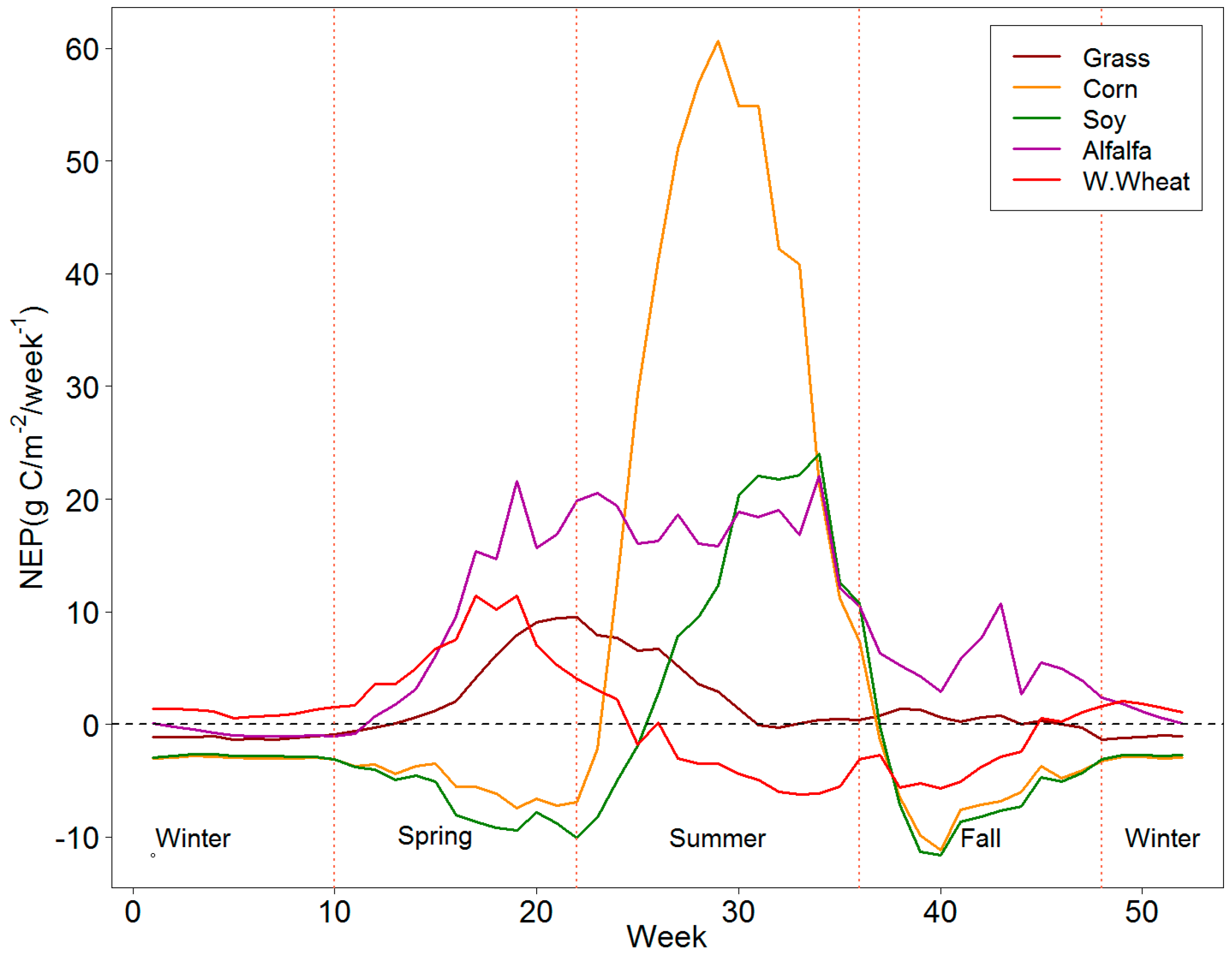
The most influential spatial variables in the NEP maps were typically those that were dynamic at the weekly time step (for example, NDVI, PAR, Week, and DOY). Precipitation (PCP), a major driver in many process-based models, had only moderate utilization in NEP modeling of 33% and 21% for grass and crop, respectively. The reduced usage or precipitation in the regression tree models may be related to the difficulty of extrapolating precipitation away from weather stations as regression tree models will only employ spatial inputs when and where they contribute to explaining the spatial or temporal variability of weekly NEP. Temperature inputs are much more reliably extrapolated away from weather stations but temperature inputs were more utilized in the crop model than the grass model. Incorporation of PAR and its high utilization in the grass model may have reduced the impact of the phenological variables (SOSN, SOST, AMP, MAXN, and EOST) relative to the crop model.

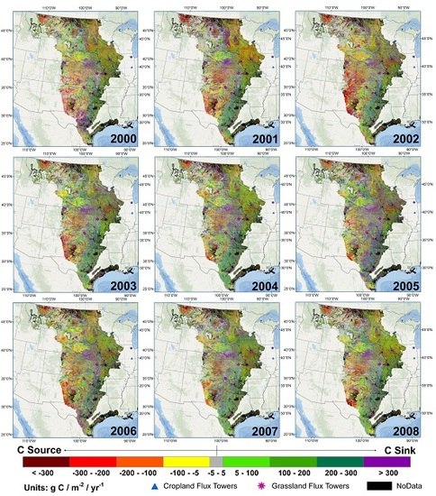
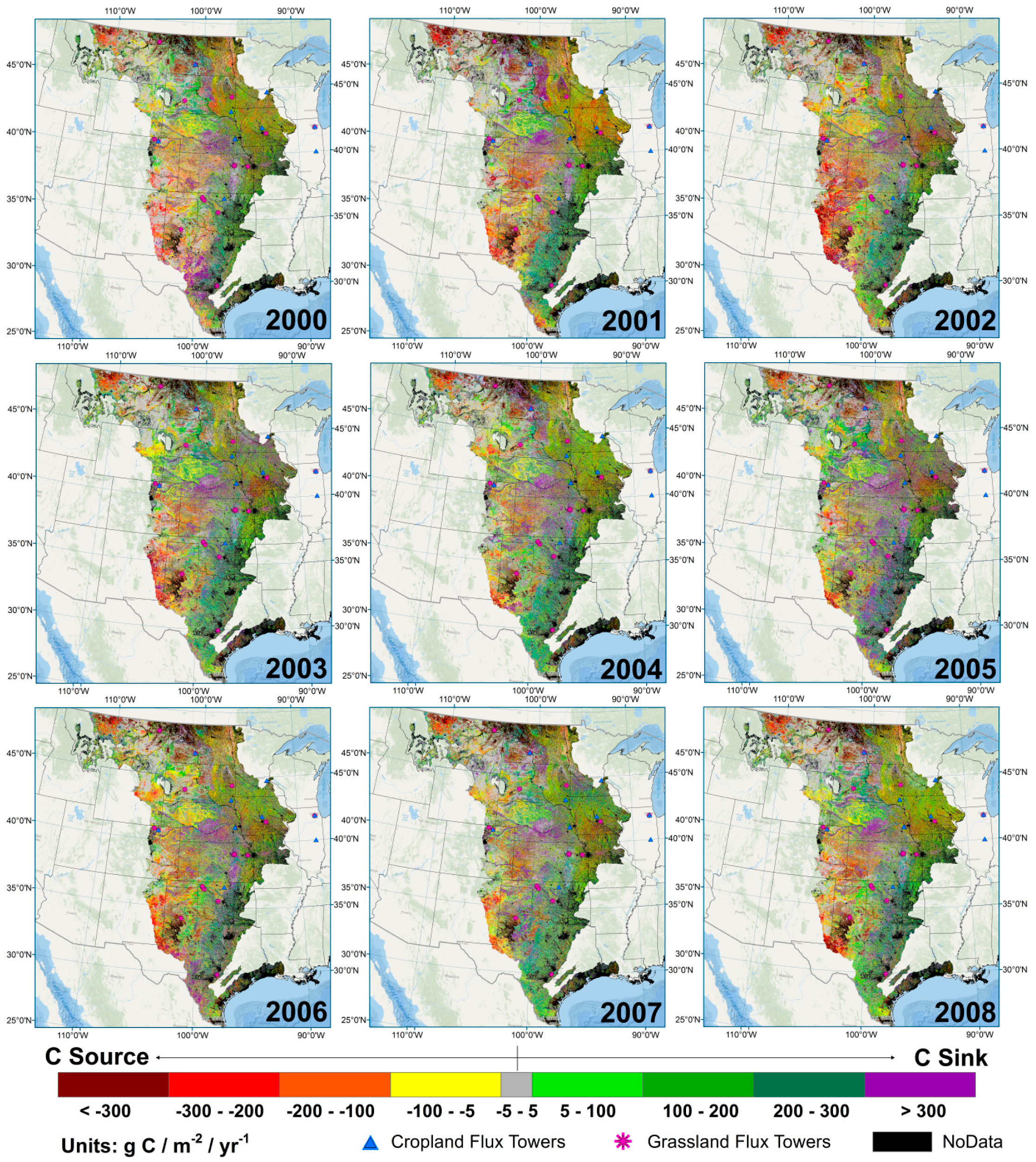
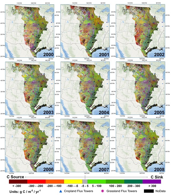
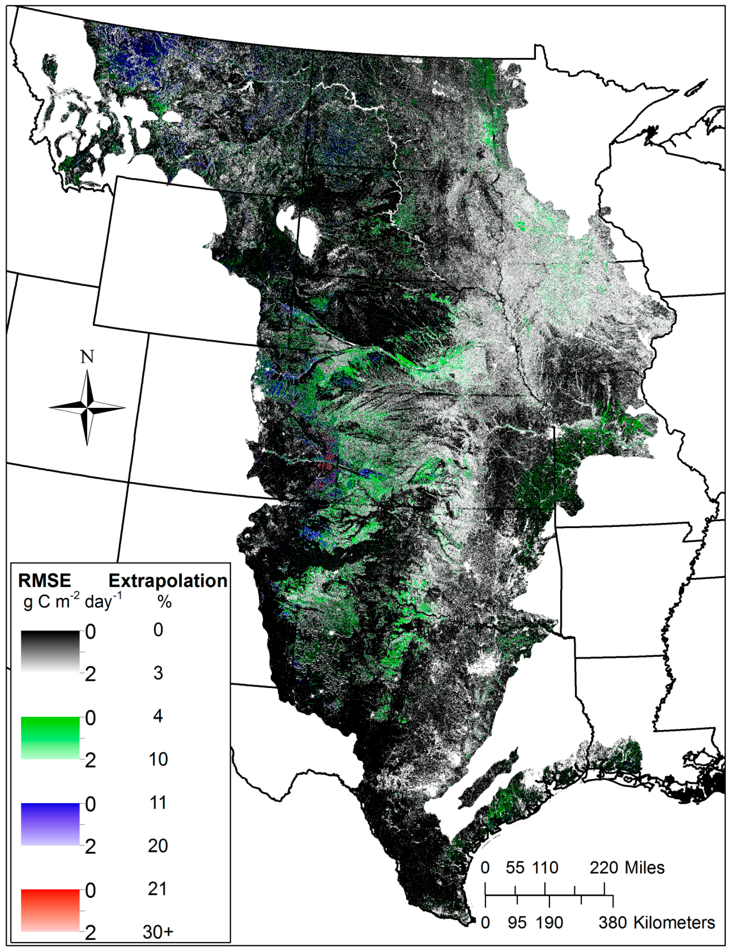
East to west moisture and productivity gradients were observed in annual and multiple year summaries (Figure 5 and Figure 7), agreeing with the general flux trends in other studies [5,11,70]. These mapping approaches provide logical and useful means to reliably extend flux tower data across space and time. Currently, available flux towers grossly under sample the Great Plains ecosystems in both time and space relative to the mapped population (area × years) of this study. The 76 site years of flux tower data used to develop the NEP mapping models represented only 0.00003% of the space for time population that was mapped (28,817,873 pixels at 250 m resolution × 9 years). Particularly, limited flux tower representation occurs in cropland areas in the extreme northern, southern, and western portions of the U.S. Great Plains (Figure 1), where high RMSE values were observed (Figure 8). Crop flux towers are primarily located in either corn or soybean fields, with little or no data available for other crops, such as cotton, spring wheat, and sorghum. Grassland areas along the southwestern edge of the Great Plains are also deficient in flux tower representation [70]. A focused expansion to the current flux tower network would improve the spatial mapping accuracies and help to ensure that extreme weather and environmental conditions are captured. Capturing extreme weather and environmental conditions with additional flux towers would result in more robust modeling results to better inform the carbon cycle science communities.

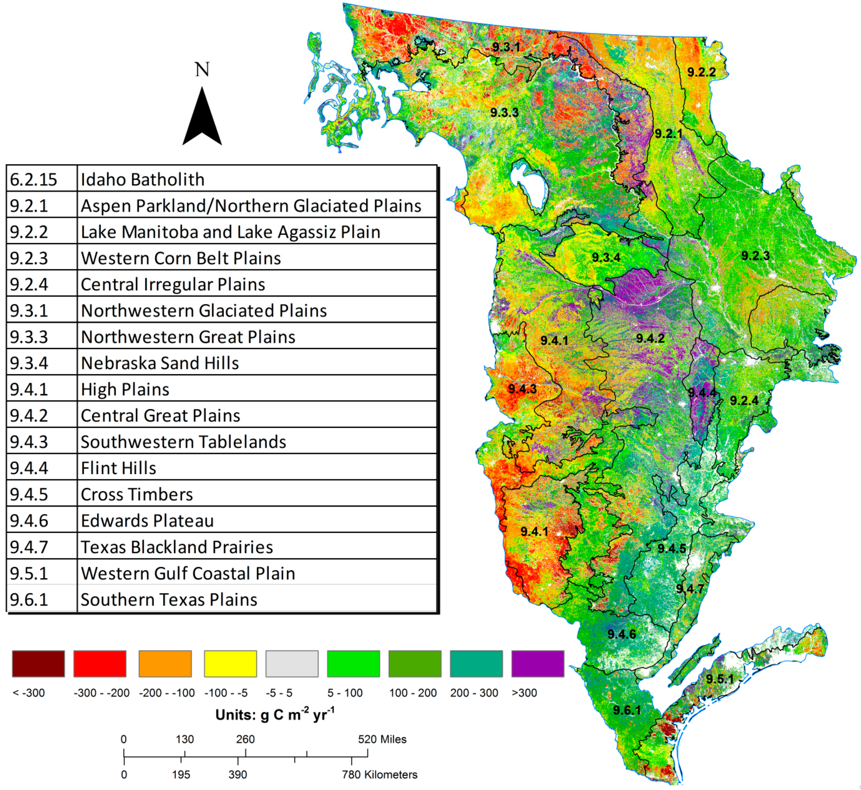
Referencing Figure 5 and Figure 7, areas with persistent high carbon sinks (>300 g C·m⁻²·year⁻¹) mapped in this study aligned with: (1) the grassland-dominated Flint Hill ecoregion (9.4.4) primarily in eastern Kansas where shallow rocky soils have allowed native tallgrass prairie systems to persist; (2) the northwestern Central Great Plains ecoregion (9.4.2) which is a mix of grassland and cropland; and (3) the eastern portions of the Northwestern Glaciated Plains ecoregion (9.3.1), a grassland-dominated region with some cropland. Another notable high carbon sink region is the edges for the Prairie Coteau in northeastern South Dakota, where steep slopes have precluded crop expansion in these grasslands which are considered by many as tallgrass systems [71].

Carbon source areas are generally aligned with the drier western edge of the Great Plains with small grain cropping in the central and western Northwestern Glaciated Plains ecoregion (9.3.1), primarily dry grasslands in the Southwestern Tablelands (9.43) and grassland and shrubland in the High Plains (9.41) ecoregion. Extreme carbon source areas (<−300 g C·m⁻²·year⁻¹) tended to be in warmer southern croplands of the Great Plains in the southeastern High Plains (9.4.1), southwestern Central Great Plains (9.4.2), and southern croplands of the Western Gulf Coastal Plain (9.51) ecoregions. These extreme flux regions are distant from the nearest crop non-wheat flux tower (Figure 1, Table S1) and may have moderate to high flux mapping uncertainties (Figure 8).

Corn production dominates the Western Corn Belt Plains ecoregion (9.2.3) transitioning from moderate carbon sinks (200 to 100 g C·m⁻²·year⁻¹) in northern and central parts of this ecoregion to moderate sources (−200 to −100 g C·m⁻²·year⁻¹) in the southern and eastern part of this ecoregion where pasture land use becomes more common in erodible soils and landscapes.

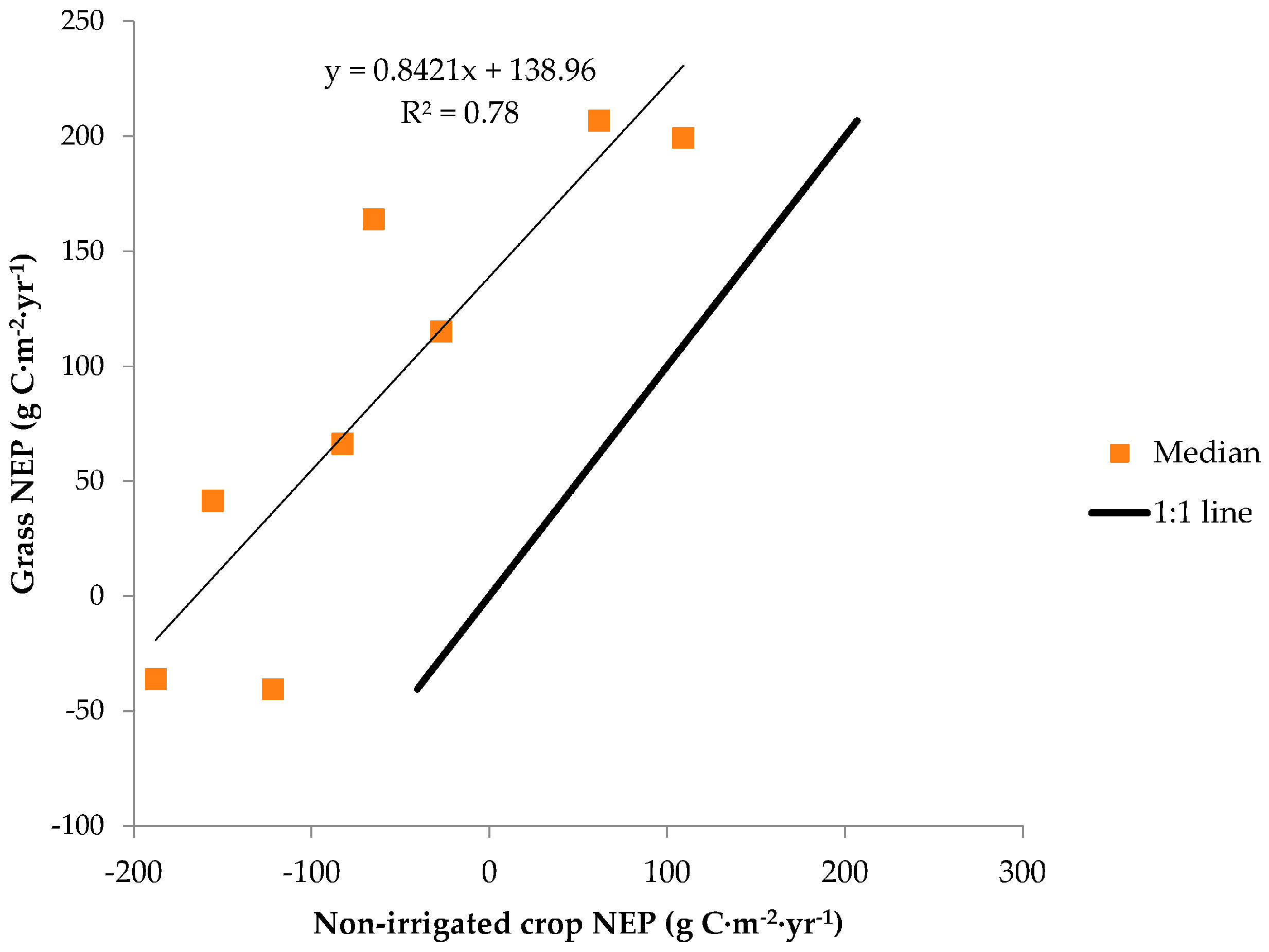
The productivity gradient analysis used regression intercept terms to quantify carbon sink advantages of grass over non-irrigated crop (Figure 12), but equilibrium NEP discussed here is from 2000 to 2008, not a long-term NEP. Given that the long-term spatial and temporal weather variations and weather extremes (very wet to strong drought years) are high in the Great Plains [72], 2000–2008 equilibrium NEP are expected to vary from the 30-year climate record (1981–2010 used in this study) and to future conditions. However, NEP productivity relationships with 30-year climate precipitation (Table 7) can help quantify expected ecosystem service benefits and consequences related to grass and non-irrigated land cover changes. Extending the carbon flux mapping period forward in time and adding more dryland crop flux tower datasets would further improve these estimates.

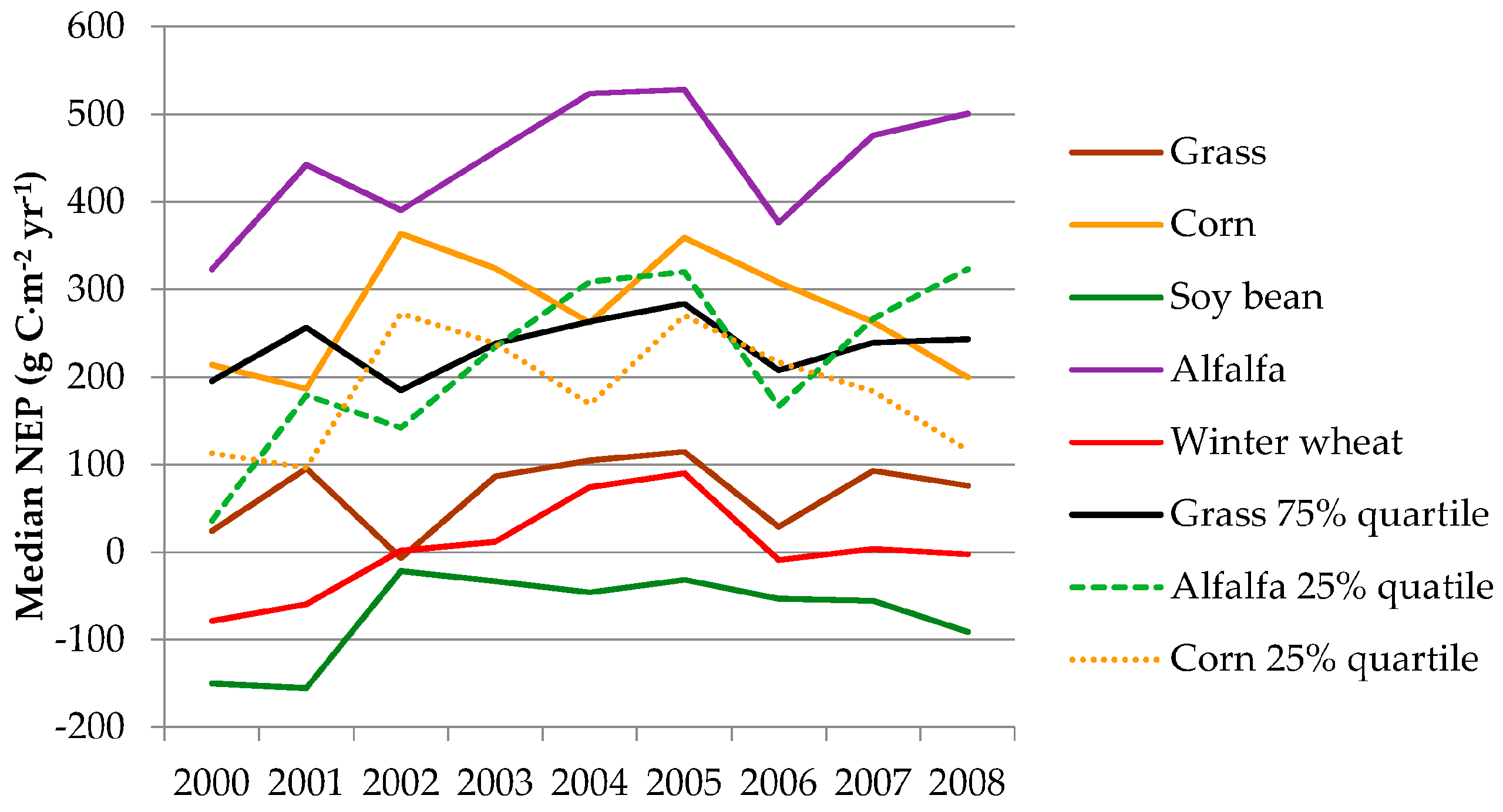
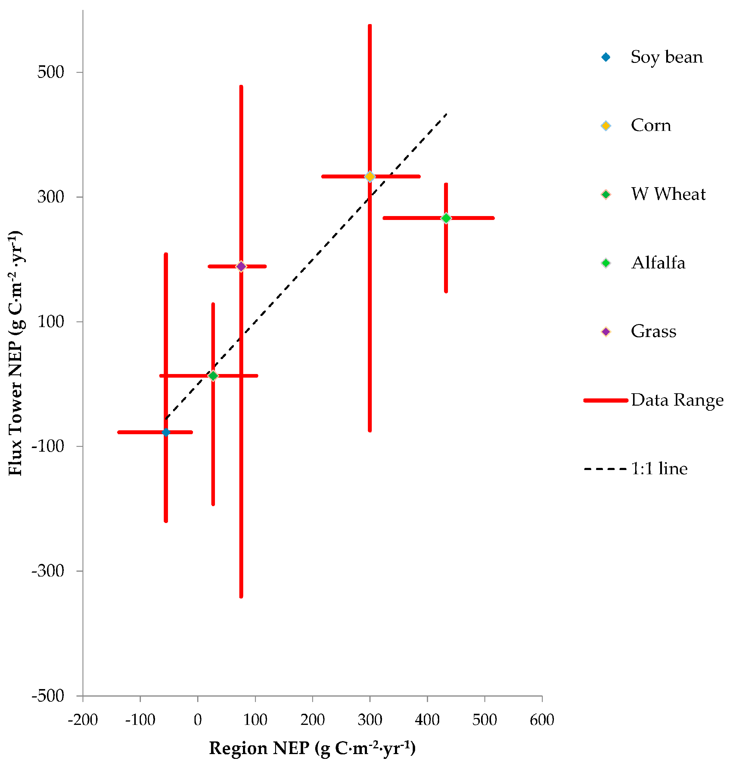
Regional Great Plains NEP means and minimum to maximum years for each majority land cover (Figure S2) through the study period agreed well with published flux tower estimates with most crop types and grass estimates, with the possible exception of alfalfa (Figure 13). Generally, individual flux tower site and year variability in NEP tended to be greater than the inter-annual variability in regional mean NEP through regional averaging and generalized fitting of the NEP mapping models for crops and grass not capturing all of the occasional flux variations. Corn-dominated regional flux means (218–385 g C·m⁻²·year⁻¹), which likely included some soybean years in the crop rotations, encompassed the mean annual corn NEP from flux towers from Gilmanov et al. [4] of 333 g C·m⁻²·year⁻¹ (Figure 13). The range of corn flux tower annual NEP observations was 121–548 g C·m⁻²·year⁻¹. Soybean-dominated areas had a long-term NEP of −56 g C·m⁻²·year⁻¹ and ranged from −137 to −12 g C·m⁻²·year⁻¹. Soybean flux tower estimates from Gilmanov, et al. [4] agreed closely with a mean NEP of −77 and a data range of −220–208 g C·m⁻²·year⁻¹. Similarly, winter wheat mean NEP was consistent (27 and 13 g C·m⁻²·year⁻¹) for regional and flux tower means, respectively. The range of annual flux estimates from regional yearly means and flux towers were comparable (−64–102 and −193–128 g C·m⁻²·year⁻¹, respectively). Grassland flux tower mean NEP was greater than the regional inter-annual mean (189 versus 75 g C·m⁻²·year⁻¹). The high variation in grass flux tower NEP is probably related to the inclusion of international grassland flux towers and because the maximum, minimum, and mean NEPs were estimated from a NEP frequency graph (Figure 11A in Gilmanov et al. [2]). Regional grassland annual means averaged across moisture and latitudinal gradients in the Great Plains tended to minimize inter-annual regional variations relative to flux tower estimates. Only alfalfa regional means and inter-annual NEP data ranges were higher than the flux tower site-year observations (Figure 13). The regional distributions of long-term alfalfa cropping are more prevalent along the drier western edge of the Great Plains and appear to be irrigation dependent due to proximities to major river systems (Arkansas, Platte, Yellowstone, and Milk Rivers, Figure S2). Flux tower alfalfa NEP estimates (5 site years) included towers east of Mandan, ND and towers in moist ecosystems (Michigan, Pennsylvania, and Italy) [3]. Recall also that alfalfa-mapped NEP was the average of the grass and crop NEP predictions (Section 2.3), which could add uncertainty. The lowest alfalfa regional annual means were in 2000 and 2002, both drier than normal years (Figure 5). Flux tower data on irrigated alfalfa in arid and semiarid ecosystems would be useful in quantifying alfalfa flux uncertainty and improving mapped NEP accuracy in these alfalfa-dominant areas.

Utilizing spatial, temporal, synoptic, remotely sensed, and ancillary digital map products to interpolate carbon fluxes through space and time is a strong approach. Our regression tree approach of using mapped versions of all input spatial variables in model development ensures that input variables are used only if prediction utility persists despite any mapping errors in the input drivers. Improved mapping of NEP fluxes would be realized with improved resolution and spatial accuracy of weather, climate, and soils information. Another limiting factor is the low density of carbon flux tower observations relative to the spatial and temporal area mapped. In particular, extreme events (droughts, wet years, early and late freezes, etc.) need to be captured to make the regression tree mapping model robust to expected and witnessed increased weather variability. Representation of major crops by flux towers is weak, particularly in non-irrigated dry environments. Regression tree mapping models should be assessed for possible over fitting or over fitting tendencies to help ensure better final map products.

Our experience has been that regression trees can be quite site specific as they are tuned to optimize prediction for a specific study area. Therefore, we do not recommend applying the Great Plains NEP mapping models in this manuscript (Tables S2 and S3) to other areas. However, we have successfully applied regression trees to subsequent (newer) years with reasonable success.

Future plans include mapping of the partitioned carbon fluxes associated with GPP and RE, which allow more functional prediction of carbon fluxes through time and space [2,3,4] than the direct mapping of the somewhat functionally confounded NEP. Further GPP and RE spatial and temporal maps would improve understanding of the causes of carbon sinks and sources. The authors intend to apply the GPP and Re mapping approach to grass and croplands across the conterminous U.S. by adding additional flux tower site years.

5. Conclusions

In this study, regression tree models were developed to estimate weekly mean daily NEP for grassland and cropland of the U.S. Great Plains for the period 2000–2008. In collecting applicable, supporting flux tower data for the study area and time frame, the final sample for mapping NEP across select grassland and cropland in the U.S. Great Plains consisted of 76 site years of flux tower data. The modeling methodology used in this study exhibited the capability for quantifying NEP at the regional level. However, a more robust flux tower network for model sampling would have been ideal for this study and several areas were identified as possible candidates for future flux tower development to better serve environmental model developers and the carbon cycle science community.

The models were applied to create weekly NEP maps at 250 m resolution for much of the cropland and grassland ecosystems in the U.S. Great Plains. Heavily used spatial inputs in the mapping models were weekly NDVI, weekly PAR, and time of year inputs (Week or DOY). The resulting map products were scaled and summarized at various temporal and spatial units and the two different land cover types were considered in a statistical, comparative analysis. Grass and cropland NEP magnitudes were similar when comparing inter-annual values. Corn and alfalfa had the strongest C stock of all the crops in this study. Grasslands showed stronger C sink tendencies (139 g·m⁻²·year⁻¹) more at the 2000–2008 NEP equilibrium than non-irrigated croplands across the moisture and productivity gradients of the Great Plains. Grassland 2000–2008 equilibrium NEP was expected to occur near 373 mm of annual precipitation from the 30-year climate record. Non-irrigated crop 2000–2008 equilibrium NEP was expected at an annual 30-year climate precipitation of 629 mm. Typically, grasslands are subject to minimal management and the soil is generally left alone, apart from occasional weed control, animal grazing, and cutting. Croplands, meanwhile, are commonly managed to control pests and weeds from the time the seed is drilled into the soil until harvest, followed by tilling, and applications of fertilizer. Higher spring and fall C retention levels in cropland soils might be observed if a cover crop was introduced to minimize soil exposure and erosion.

The maps and statistics presented in this study provide a framework and basic overview of C fluctuations in the U.S. Great Plains throughout the 2000–2008 time frame. This effort is expected to be continued and to be expanded to include cropland and grassland for the entire conterminous U.S. and possibly include NEP estimates for additional years and/or other land cover types, such as forests and shrublands. Understanding and being able to visualize the carbon cycling as a function of land cover and land use will help drive decision making in the area of land management and promote natural resource sustainability.

References

1. Blühdorn, I. The politics of unsustainability: COP15, post-ecologism, and the ecological paradox. Organ. Environ. 2011. [Google Scholar] [CrossRef]
2. Gilmanov, T.G.; Aires, L.; Barcza, Z.; Baron, V.S.; Belelli, L.; Beringer, J.; Billesbach, D.; Bonal, D.; Bradford, J.; Ceschia, E.; et al. Productivity, respiration, and light-response parameters of world grassland and agroecosystems derived from flux-tower measurements. Rangel. Ecol. Manag. 2010, 63, 16–39. [Google Scholar] [CrossRef]
3. Gilmanov, T.G.; Baker, J.M.; Bernacchi, C.J.; Billesbach, D.P.; Burba, G.G.; Castro, S.; Chen, J.; Eugster, W.; Fischer, M.L.; Gamon, J.A.; et al. Productivity and carbon dioxide exchange of leguminous crops: Estimates from flux tower measurements. Agron. J. 2014, 106, 545–559. [Google Scholar] [CrossRef]
4. Gilmanov, T.G.; Wylie, B.K.; Tieszen, L.L.; Meyers, T.P.; Baron, V.S.; Bernacchi, C.J.; Billesbach, D.P.; Burba, G.G.; Fischer, M.L.; Glenn, A.J.; et al. CO2 uptake and ecophysiological parameters of the grain crops of midcontinent North America: Estimates from flux tower measurements. Agric. Ecosyst. Environ. 2013, 164, 162–175. [Google Scholar] [CrossRef]
5. Xiao, J.; Ollinger, S.V.; Frolking, S.; Hurtt, G.C.; Hollinger, D.Y.; Davis, K.J.; Pan, Y.; Zhang, X.; Deng, F.; Chen, J.; et al. Data-driven diagnostics of terrestrial carbon dynamics over North America. Agric. For. Meteorol. 2014, 197, 142–157. [Google Scholar] [CrossRef]
6. Liang, S. Recent advances in land remote sensing: An overview. In Advances in Land Remote Sensing: System, Modeling, Inversion and Application; Liang, S., Ed.; Springer: Berlin, Germany, 2008; pp. 1–8. [Google Scholar]
7. Pastick, N.J.; Jorgenson, M.T.; Wylie, B.K.; Rose, J.R.; Rigge, M.; Walvoord, M.A. Spatial variability and landscape controls of near-surface permafrost within the Alaskan Yukon River Basin. J. Geophys. Res. Biogeosci. 2014, 119, 1244–1265. [Google Scholar] [CrossRef]
8. Pastick, N.J.; Rigge, M.; Wylie, B.K.; Jorgenson, M.T.; Rose, J.R.; Johnson, K.D.; Ji, L. Distribution and landscape controls of organic layer thickness and carbon within the Alaskan Yukon River Basin. Geoderma 2014, 230–231, 79–94. [Google Scholar] [CrossRef]
9. Running, S.W.; Nemani, R.R.; Heinsch, F.A.; Zhao, M.; Reeves, M.; Hashimoto, H. A continuous satellite-derived measure of global terrestrial primary production. BioScience 2004, 54, 547–560. [Google Scholar] [CrossRef]
10. Wylie, B.K.; Fosnight, E.A.; Gilmanov, T.G.; Frank, A.B.; Morgan, J.A.; Haferkamp, M.R.; Meyers, T.P. Adaptive data-driven models for estimating carbon fluxes in the Northern Great Plains. Remote Sens. Environ. 2007, 106, 399–413. [Google Scholar] [CrossRef]
11. Zhang, L.; Wylie, B.K.; Ji, L.; Gilmanov, T.G.; Tieszen, L.L.; Howard, D.M. Upscaling carbon fluxes over the Great Plains grasslands: Sinks and sources. J. Geophys. Res. Biogeosci. 2011, 116. [Google Scholar] [CrossRef]
12. Wagle, P.; Xiao, X.; Scott, R.L.; Kolb, T.E.; Cook, D.R.; Brunsell, N.; Baldocchi, D.D.; Basara, J.; Matamala, R.; Zhou, Y.; et al. Biophysical controls on carbon and water vapor fluxes across a grassland climatic gradient in the United States. Agric. For. Meteorol. 2015, 214–215, 293–305. [Google Scholar] [CrossRef]
13. Jung, M.; Reichstein, M.; Bondeau, A. Towards global empirical upscaling of FLUXNET eddy covariance observations: Validation of a model tree ensemble approach using a biosphere model. Biogeosciences 2009, 6, 2001–2013. [Google Scholar] [CrossRef]
14. Wylie, B.K.; Johnson, D.A.; Laca, E.; Saliendra, N.Z.; Gilmanov, T.G.; Reed, B.C.; Tieszen, L.L.; Worstell, B.B. Calibration of remotely sensed, coarse resolution NDVI to CO2 fluxes in a sagebrush–steppe ecosystem. Remote Sens. Environ. 2003, 85, 243–255. [Google Scholar] [CrossRef]
15. Ahlström, A.; Raupach, M.R.; Schurgers, G.; Smith, B.; Arneth, A.; Jung, M.; Reichstein, M.; Canadell, J.G.; Friedlingstein, P.; Jain, A.K.; et al. The dominant role of semi-arid ecosystems in the trend and variability of the land CO2 sink. Science 2015, 348, 895–899. [Google Scholar] [CrossRef] [PubMed]
16. Liu, S.; Tan, Z.; Chen, M.; Liu, J.; Wein, A.; Li, Z.; Huang, S.; Oeding, J.; Young, C.; Verma, S.B.; et al. Chapter 18—The General Ensemble Biogeochemical Modeling System (GEMS) and its Applications to Agricultural Systems in the United States A2. In Managing Agricultural Greenhouse Gases; Follett, R.F., Liebig, M., Franzluebbers, A.J., Eds.; Academic Press: San Diego, CA, USA, 2012; pp. 309–323. [Google Scholar]
17. Eve, M.D.; Sperow, M.; Paustian, K.; Follett, R.F. National-scale estimation of changes in soil carbon stocks on agricultural lands. Environ. Pollut. 2002, 116, 431–438. [Google Scholar] [CrossRef]
18. Xiao, J.; Zhuang, Q.; Law, B.E.; Baldocchi, D.D.; Chen, J.; Richardson, A.D.; Melillo, J.M.; Davis, K.J.; Hollinger, D.Y.; Wharton, S.; et al. Assessing net ecosystem carbon exchange of U.S. terrestrial ecosystems by integrating eddy covariance flux measurements and satellite observations. Agric. For. Meteorol. 2011, 151, 60–69. [Google Scholar] [CrossRef]
19. De’ath, G.; Fabricius, K.E. Classification and regression trees: A powerful yet simple technique for ecological data analysis. Ecology 2000, 81, 3178–3192. [Google Scholar] [CrossRef]
20. Quinlan, J.R. Learning with continuous classes. In Proceedings of the 5th Australian Joint Conference on Artificial Intelligence, Hobart, Tasmania, 16–18 November 1992; pp. 343–348.
21. Fry, J.A.; Xian, G.; Jin, S.; Dewitz, J.A.; Homer, C.G.; Yang, L.; Barnes, C.A.; Herold, N.D.; Wickham, J.D. Completion of the 2006 National Land Cover Database for the conterminous United States. Photogramm. Eng. Remote Sens. 2011, 77, 858–864. [Google Scholar]
22. North American Carbon Program. About NACP. Available online: http://nacarbon.org/nacp/about.html (accessed on 4 January 2016).
23. FLUXNET. Home Page. Available online: http://fluxnet.ornl.gov/ (accessed on 4 January 2016).
24. Aubinet, M.; Vesala, T.; Papale, D. Eddy Covariance: A Practical Guide to Measurement and Data Analysis; Springer Science & Business Media: New York, NY, USA, 2012. [Google Scholar]
25. Stoy, P.C.; Katul, G.G.; Siqueira, M.B.; Juang, J.-Y.; Novick, K.A.; Uebelherr, J.M.; Oren, R. An evaluation of models for partitioning eddy covariance-measured net ecosystem exchange into photosynthesis and respiration. Agric. For. Meteorol. 2006, 141, 2–18. [Google Scholar] [CrossRef]
26. Jenkerson, C.B.; Maiersperger, T.K.; Schmidt, G.L. eMODIS: A User-Friendly Data Source; U.S. Geological Survey Open-File Report 2010–1055; USGS: Reston, VA, USA, 2010. Available online: http://pubs.er.usgs.gov/publication/ofr20101055 (accessed on 11 November 2014).
27. Ollinger, S.V. Sources of variability in canopy reflectance and the convergent properties of plants. New Phytol. 2011, 189, 375–394. [Google Scholar] [CrossRef] [PubMed]
28. Brown, J.; Howard, D.; Wylie, B.; Frieze, A.; Ji, L.; Gacke, C. Application-ready expedited MODIS data for operational land surface monitoring of vegetation condition. Remote Sens. 2015, 7, 16226–16240. [Google Scholar] [CrossRef]
29. Swets, D.L.; Reed, B.C.; Rowland, J.D.; Marko, S.E. A weighted least-squares approach to temporal NDVI smoothing. In Proceedings of the 1999 ASPRS Annual Conference, Portland, OR, USA, 17–21 May 1999; pp. 526–536.
30. Krofcheck, D.; Eitel, J.; Lippitt, C.; Vierling, L.; Schulthess, U.; Litvak, M. Remote sensing based simple models of GPP in both disturbed and undisturbed piñon-juniper woodlands in the southwestern U.S. Remote Sens. 2015, 8, 20. [Google Scholar] [CrossRef]
31. Gu, Y.; Wylie, B.K.; Howard, D.M.; Phuyal, K.P.; Ji, L. NDVI saturation adjustment: A new approach for improving cropland performance estimates in the Greater Platte River Basin, USA. Ecol. Indic. 2013, 30, 1–6. [Google Scholar] [CrossRef]
32. National Weather Service. National Centers for Environmental Prediction. Available online: http://www.ncep.noaa.gov (accessed on 11 November 2014).
33. PRISM Climate Group. PRISM Climate Data. Available online: http://prism.oregonstate.edu (accessed on 12 January 2016).
34. Reed, B.C.; Brown, J.F.; Vanderzee, D.; Loveland, T.R.; Merchant, J.W.; Ohlen, D.O. Measuring phenological variability from satellite imagery. J. Veg. Sci. 1994, 5, 703–714. [Google Scholar] [CrossRef]
35. U.S. Geological Survey. Remote Sensing Phenology. Available online: http://phenology.cr.usgs.gov/ (accessed on 4 January 2016).
36. Natural Resources Conservation Service. SSURGO/STATSGO2 Structural Metadata and Documentation. Available online: http://www.nrcs.usda.gov/wps/portal/nrcs/detail/soils/home/?cid=nrcs142p2_053631 (accessed on 11 November 2014).
37. Howard, D.M.; Wylie, B.K. Annual crop type classification of the US Great Plains for 2000 to 2011. Photogramm. Eng. Remote Sens. 2014, 80, 537–549. [Google Scholar] [CrossRef]
38. Omernik, J.M. Ecoregions of the conterminous United States. Annn. Assoc. Am. Geogr. 1987, 77, 118–125. [Google Scholar] [CrossRef]
39. USDA Natural Resources Conservation Service. Major Land Resource Area (MLRA). Available online: http://www.nrcs.usda.gov/wps/portal/nrcs/detail/soils/survey/?cid=nrcs142p2_053624 (accessed on 12 January 2016).
40. USGS Early Warning and Environmental Monitoring Program. Moderate Resolution Imaging Spectroradiometer (MODIS) Irrigated Agriculture Dataset for the United States (MIrAD-US). Available online: http://earlywarning.usgs.gov/USirrigation (accessed on 12 January 2016).
41. RuleQuest Research. Rulequest Research: Data Mining Tools. Available online: http://www.rulequest.com (accessed on 11 November 2014).
42. Brown, J.F.; Wardlow, B.D.; Tadesse, T.; Hayes, M.J.; Reed, B.C. The Vegetation Drought Response Index (VegDRI): A new integrated approach for monitoring drought stress in vegetation. GISci. Remote Sens. 2008, 45, 16–46. [Google Scholar] [CrossRef]
43. Gu, Y.; Wylie, B.K. Developing a 30-m grassland productivity estimation map for central Nebraska using 250-m MODIS and 30-m Landsat-8 observations. Remote Sens. Environ. 2015, 171, 291–298. [Google Scholar] [CrossRef]
44. Homer, C.; Huang, C.; Yang, L.; Wylie, B.; Coan, M. Development of a 2001 National Land-Cover Database for the United States. Photogramm. Eng. Remote Sens. 2004, 70, 829–840. [Google Scholar] [CrossRef]
45. Homer, C.G.; Aldridge, C.L.; Meyer, D.K.; Schell, S.J. Multi-scale remote sensing sagebrush characterization with regression trees over Wyoming, USA: Laying a foundation for monitoring. Int. J. Appl. Earth Obs. Geoinf. 2012, 14, 233–244. [Google Scholar] [CrossRef]
46. Homer, C.G.; Aldridge, C.L.; Meyer, D.K.; Schell, S.J. Multiscale Sagebrush Rangeland Habitat Modeling in the Gunnison Basin of Colorado; US Geological Survey: Reston, VA, USA, 2013.
47. Ji, L.; Wylie, B.K.; Nossov, D.R.; Peterson, B.; Waldrop, M.P.; McFarland, J.W.; Rover, J.; Hollingsworth, T.N. Estimating aboveground biomass in interior Alaska with Landsat data and field measurements. Int. J. Appl. Earth Obs. Geoinf. 2012, 18, 451–461. [Google Scholar] [CrossRef]
48. Peterson, B.; Nelson, K.; Wylie, B. Towards integration of GLAS into a national fuel mapping program. Photogramm. Eng. Remote Sens. 2013, 79, 175–183. [Google Scholar] [CrossRef]
49. Rollins, M.G. LANDFIRE: A nationally consistent vegetation, wildland fire, and fuel assessment. Int. J. Wildland Fire 2009, 18, 235–249. [Google Scholar] [CrossRef]
50. Rover, J.; Wylie, B.K.; Ji, L. A self-trained classification technique for producing 30 m percent-water maps from Landsat data. Int. J. Remote Sens. 2010, 31, 2197–2203. [Google Scholar] [CrossRef]
51. Wylie, B.K.; Zhang, L.; Bliss, N.; Ji, L.; Tieszen, L.L.; Jolly, W.M. Integrating modelling and remote sensing to identify ecosystem performance anomalies in the boreal forest, Yukon River Basin, Alaska. Int. J. Digit. Earth 2008, 1, 196–220. [Google Scholar] [CrossRef]
52. Cawley, G.C.; Talbot, N.L. Fast exact leave-one-out cross-validation of sparse least-squares support vector machines. Neural Netw. 2004, 17, 1467–1475. [Google Scholar] [CrossRef] [PubMed]
53. Chapelle, O.; Vapnik, V.; Bousquet, O.; Mukherjee, S. Choosing multiple parameters for support vector machines. Mach. Learn. 2002, 46, 131–159. [Google Scholar] [CrossRef]
54. Keele, L.; Kelly, N.J. Dynamic models for dynamic theories: The ins and outs of lagged dependent variables. Political Anal. 2006, 14, 186–205. [Google Scholar] [CrossRef]
55. Vapnik, V.; Chapelle, O. Bounds on error expectation for support vector machines. Neural Comput. 2000, 12, 2013–2036. [Google Scholar] [CrossRef] [PubMed]
56. Ji, L.; Wylie, B.K.; Brown, D.R.; Peterson, B.; Alexander, H.D.; Mack, M.C.; Rover, J.; Waldrop, M.P.; McFarland, J.W.; Chen, X. Spatially explicit estimation of aboveground boreal forest biomass in the Yukon River Basin, Alaska. Int. J. Remote Sens. 2015, 36, 939–953. [Google Scholar] [CrossRef]
57. De’Ath, G. Multivariate regression trees: A new technique for modeling species-environment relationships. Ecology 2002, 83, 1105–1117. [Google Scholar]
58. Hsu, C.-W.; Chang, C.-C.; Lin, C.-J. A Practical Guide to Support Vector Classification; Technical Report; Department of Computer Science, National Taiwan University: Taipei, Taiwan, 2003. [Google Scholar]
59. Briscoe, E.; Feldman, J. Conceptual complexity and the bias/variance tradeoff. Cognition 2011, 118, 2–16. [Google Scholar] [CrossRef] [PubMed]
60. Gu, Y.; Wylie, B.K.; Boyte, S.P.; Picotte, J.J.; Howard, D.M.; Smith, K.; Nelson, K.J. An optimal sample data usage strategy to minimize overfitting and underfitting effects in regression tree models based on remotely sensed data. Remote Sens. 2016, 8, 943. [Google Scholar] [CrossRef]
61. Papale, D.; Black, T.A.; Carvalhais, N.; Cescatti, A.; Chen, J.Q.; Jung, M.; Kiely, G.; Lasslop, G.; Mahecha, M.D.; Margolis, H.; et al. Effect of spatial sampling from European flux towers for estimating carbon and water fluxes with artificial neural networks. J. Geophys. Res. Biogeosci. 2015, 120, 1941–1957. [Google Scholar] [CrossRef]
62. Tieszen, L.L.; Reed, B.C.; Bliss, N.B.; Wylie, B.K.; DeJong, D.D. NDVI, C3 and C4 production, and distributions in Great Plains grassland land cover classes. Ecol. Appl. 1997, 7, 59–78. [Google Scholar]
63. Brown, J.F.; Pervez, M.S. Merging remote sensing data and national agricultural statistics to model change in irrigated agriculture. Agric. Syst. 2014, 127, 28–40. [Google Scholar] [CrossRef]
64. Alexander, C. Quantitative Methods in Finance; Wiley: Hoboken, NJ, USA, 2008. [Google Scholar]
65. McCulloch, J.H. Median-unbiased estimation of higher order autoregressive/unit root processes and autocorrelation consistent covariance estimation in a money demand model. In 2008 North American Summer Meetings; Econometric Society: Pittsburgh, PA, USA, 2008. [Google Scholar]
66. U.S. Drought Monitor, Map Archive. U.S. Drought Monitor CONUS. Available online: http://droughtmonitor.unl.edu/MapsAndData/MapArchive.aspx (accessed on 18 May 2016).
67. U.S. Geological Survey. U.S. Great Plains NEP—250 m Raster Data. Available online: http://lca.usgs.gov/lca/cflux_gplains/dataproducts.php (accessed on 12 May 2016).
68. U.S. Geological Survey. Carbon Flux Quantification in the Great Plains. Available online: http://lca.usgs.gov/lca/cflux_gplains/dataproducts.php (accessed on 10 November 2016).
69. Zhang, L.; Wylie, B.K.; Ji, L.; Gilmanov, T.G.; Tieszen, L.L. Climate-driven interannual variability in net ecosystem exchange in the northern Great Plains grasslands. Rangel. Ecol. Manag. 2010, 63, 40–50. [Google Scholar] [CrossRef]
70. Gu, Y.; Howard, D.M.; Wylie, B.K.; Zhang, L. Mapping carbon flux uncertainty and selecting optimal locations for future flux towers in the Great Plains. Landsc. Ecol. 2012, 27, 319–326. [Google Scholar] [CrossRef]
71. Holechek, J.L.; Pieper, R.D.; Herbel, C.H. Range Management: Principles and Practices; Prentice-Hall: Upper Saddle River, NJ, USA, 1995. [Google Scholar]
72. White, A.B.; Kumar, P.; Tcheng, D. A data mining approach for understanding topographic control on climate-induced inter-annual vegetation variability over the United States. Remote Sens. Environ. 2005, 98, 1–20. [Google Scholar] [CrossRef]
Figure 1. The map of the Great Plains with the National Land Cover Database (NLCD) 2006 as the backdrop, along with grassland and cropland flux towers used in this study as green and yellow points. Numbered flux tower labels refer to individual flux towers as designated in Table S1. Source: [21].
Remotesensing 08 00944 g001
Figure 2. Rangeland productivity strata (above ground biomass) classes for a normal year.
Remotesensing 08 00944 g002
Figure 3. Crop mapping model randomized test and training variations in mean (of nine replications) MAD as a function of the size of the training dataset.
Remotesensing 08 00944 g003
Figure 4. Grassland NEP mapping model randomized test and training mean (from nine replications) error terms (MAD) with varying test sizes.
Remotesensing 08 00944 g004
Figure 5. Cumulative annual NEP of the U.S. Great Plains for 2000–2008 [67]. Data published at [68].
Remotesensing 08 00944 g005
Figure 6. Cumulative seasonal NEP of the U.S. Great Plains for 2000–2008.
Remotesensing 08 00944 g006
Figure 7. Mean annual NEP map (2000–2008) with overlaid Level 3 Ecoregions. The spatial mean of cropland NEP for the U.S. Great Plains was calculated to be 30.63 g C·m−2·year−1 and the spatial mean of grassland NEP was calculated to be 45.37 g C·m−2·year−1.
Remotesensing 08 00944 g007
Figure 8. Distribution of leave-one-out site cross validation RMSE and degree of extrapolation.
Remotesensing 08 00944 g008
Figure 9. NEP comparison of all crops and grasslands through time. Note that these are median values because of non-normality in some year and class combinations whereas the grass and crop NEP values reported in Figure 7 are inter-annual means.
Remotesensing 08 00944 g009
Figure 10. Major crop type NEP comparisons to grassland NEP.
Remotesensing 08 00944 g010
Figure 11. Mean weekly NEP based on land cover type in the U.S. Great Plains (2000–2008).
Remotesensing 08 00944 g011
Figure 12. Grass NEP regressed on non-irrigated crop NEP using regional class rangeland biomass median 2000–2008 mean NEP.
Remotesensing 08 00944 g012
Figure 13. Agreement of NEP between flux tower synthesis analysis [2,3,4] and regional dominant land cover mapped areas.
Remotesensing 08 00944 g013