Urban Heat Islands as Viewed by Microwave Radiometers and Thermal Time Indices

Abstract

Urban heat islands (UHIs) have been long studied using both ground-based observations of air temperature and remotely sensed thermal infrared (TIR) data. While ground-based observations lack spatial detail even in the occasional “dense” urban network, skin temperature retrievals using TIR data have lower temporal coverage due to revisit frequency, limited swath width, and cloud cover. Algorithms have recently been developed to retrieve near-surface air temperatures using microwave radiometer data, which enables characterization of UHIs in metropolitan areas, major conurbations, and global megacities at regional to continental scales using temporally denser time series than those that have been available from TIR sensors. Here we examine how UHIs appear across the entire Western Hemisphere using surface air temperatures derived from the Advanced Microwave Scanning Radiometers (AMSRs), AMSR-E onboard the National Aeronautics and Space Administration’s (NASA’s) Aqua and AMSR2 onboard the Japan Aerospace eXploration Agency’s Global Change Observation Mission-Water1 (JAXA’s GCOM-W1) satellites. We compare these data with station observations from the Global Historical Climate Network (GHCN) for 27 major cities across North America (in 83 urban-rural groupings) to demonstrate the capability of microwave data in a UHI study. Two measures of thermal time, accumulated diurnal and nocturnal degree-days, are calculated from the remotely sensed surface air temperature time series to characterize the urban-rural thermal differences over multiple growing seasons. Daytime urban thermal accumulations from the microwave data were sometimes lower than in adjacent rural areas. In contrast, station observations showed consistently higher day and night thermal accumulations in cities. UHIs are more pronounced at night, with 55% (AMSRs) and 93% (GHCN) of urban-rural groupings showing higher accumulated nocturnal degree-days in cities. While urban-rural thermal gradients may vary according to different datasets or locations, day-night differences in thermal time metrics were consistently lower (>90% of urban-rural groupings) in urban areas than in rural areas for both datasets. We propose that the normalized difference accumulated thermal time index (NDATTI) is a more robust metric for comparative UHI studies than simple temperature differences because it can be calculated from either station or remotely sensed data and it attenuates latitudinal effects.

1. Introduction

The world’s population has become increasingly urban over the past two centuries. In 1800, only 2% of the world’s population lived in cities [1]. By 1950, the world’s urban fraction grew to 30% [2]. By 2014, more than half the world (54%) resided in urbanized areas. The world’s urban population grew rapidly from 746 million in 1950 to 3.9 billion in 2014. As the planetary surface continues to urbanize, about 6.4 billion people are predicted to live in cities by 2050, accounting for 66% of the global population. Urbanization strongly affects local surface energy, water, and carbon budgets, thereby impacting climate and ecosystems at multiple scales [3,4,5,6]. The urban heat island (UHI) effect refers to the modified thermal climate in urbanized areas compared to nearby rural areas, and the UHI is a prime example of micro- to mesoscale anthropogenic climate modification.

The urban heat island is mainly caused by differences in heat capacities of urban and rural land covers [7,8,9]. During the day, building materials in the city generally absorb more incoming solar radiation than vegetation and soils in the adjacent countryside due to their higher heat capacity, resulting in higher temperatures in the city. The difference between urban and rural temperature is pronounced at night when the urban infrastructure radiates the shortwave solar energy absorbed during the day as longwave thermal infrared (TIR) radiation. Other contributors to UHI including anthropogenic heating sources, including outdoor lighting, motor vehicles, heating, ventilation, and air-conditioning (HVAC) systems, and industrial facilities.

Urban heat islands have been studied in individual cities using ground-based observations taken from weather station networks or by traverses with thermometers mounted on vehicles. Near-surface air temperatures at a nominal height of two meters have the advantage of a high temporal resolution and a long data record, but they lack of spatial detail, even in the occasional “dense” urban network [7,10,11,12]. Since the advent of remote sensing technology in the 1970s, radiometric land surface temperature (LST) over large areas has been available from spaceborne and airborne platforms [11,12,13]. TIR (11–14 µm) data are used for most LST retrievals. A variety of orbital sensors has been developed to collect TIR data such as Landsat TM/ETM+/TIRS, AVHRR, MODIS, and ASTER. In contrast to in situ measurements that can monitor on the scale of minutes the temperature variations at specific locations, TIR observations from orbital sensors are constrained by obscuring cloud cover, sensor swath width, and overpass frequency. Hence, TIR-based UHI studies are often conducted using relatively few temporal observations that are spatially comprehensive, but at coarse spatial resolution relative to the components in the built environment. Missing or out of range observations due to cloud cover, sensor artifacts, or unusual events (e.g., active fires) can also pose problems for systematic comparisons of UHIs over large areas.

Recent advances in the processing of passive microwave radiometer data have yielded products that measure a range of biogeophysical variables at the surface, including air temperature [14,15,16]. Despite the coarse spatial resolution of these data (25 km grids) and the inability to retrieve temperatures over frozen surfaces, the terrestrial radiation at microwave frequencies penetrates most clouds and enables observations at nighttime. Thus, microwave products can provide more views of the surface, albeit at reduced spatial resolution.

Although early attempts to retrieve surface temperature using microwave data dated back to the 1990s, retrievals are only available for some regions during limited periods [17,18,19]. Not until recently [14,15,16] global near-surface air temperatures estimated from microwave data available using on a near-daily basis for more than a decade. The Advanced Microwave Scanning Radiometer-Earth observing system (AMSR-E) on the Aqua satellite provided high temporal resolution views of land surface and boundary layer properties until antenna failure in October 2011. A blended dataset was recently produced that combines the AMSR-E data with data from AMSR2 that was launched on GCOM-W1 in May 2012 [16]. The data gap has been filled using Microwave Radiation Imager (MWRI), the microwave radiometer on the Chinese satellite FengYun-3B (FY3B) [20]. This blended dataset offers a great opportunity to analyze UHIs associated with metropolitan areas, major conurbations, and global megacities at a scale not previously considered. The equatorial overpass times on the ascending node is 1330 for AMSR-E and AMSR2 and 1340 for MWRI; thus, there is little difference in acquisition times.

Taking advantage of this global high temporal resolution surface air temperature time series, we are able to visualize how UHIs appear during the frost-free period across the entire Western Hemisphere. We quantify seasonal differences in thermal regimes between urban and surrounding rural areas using metrics of thermal time and their accumulations over the growing season. We compare AMSR-derived accumulated thermal times with those calculated from station observations for major urban areas across North America. Our preliminary results indicate that day-night thermal differences may be better indicators across different land surfaces than daytime or nighttime temperatures. Thus, we propose and investigate a new index—the normalized difference accumulated thermal time index (NDATTI)—to characterize long-term thermal dynamics across large areas and to attenuate latitudinal effects in order to facilitate comparative studies of the UHI.

2. Materials and Methods

2.1. Study Region

We focused on major urban areas of the Western Hemisphere and nearby rural areas. Due to the coarse spatial resolution of the AMSR surface air temperature product, only the largest inland cities can generate a distinct UHI. As the algorithms do not function over open water, coastal cities are generally not visible. Table S1 lists the largest conurbations and megacities in the Western Hemisphere by size and their estimated population in 2016 [21].

2.2. Surface Air Temperature

Temperature retrievals from the AMSR data could only be retreived over land for non-precipitating, non-snow, and non-ice covered conditions [14,15,16]. Therefore, we analyzed the surface air temperature data from the period between the vernal and autumnal equinoxes: approximately 21 March to 23 September in the Northern Hemisphere, and 23 September to 21 March in the southern Hemisphere.

2.2.1. AMSR Data

AMSR measures V and H polarized brightness temperature (Tb) at six frequencies, scanning conically in the forward direction at a constant incidence angle of 55° from nadir. The primary inputs used to derive near surface daily air temperature minima and maxima (Tmin and Tmax) over land are daily 18.7 and 23.8 GHz dual polarized brightness temperatures (version 3) obtained in global 25-km Equal-Area Scalable Earth (EASE) grid format from the National Snow and Ice Data Center (NSIDC) (Boulder, CO, USA). Temporal coverage for the data products is from 19 June 2002 through 31 December 2014 [14,15,16]. Retrieved surface air temperatures have been extensively compared to World Meteorological Organization (WMO) station observations and Atmospheric Infrared Sounder/Advanced Microwave Sounding Unit (AIRS/AMSU) surface air temperature retrievals for the Northern Hemisphere [22]. Accuracy is consistent across latitudes but varies significantly among land use types. AMSR derived air temperatures are within approximately 3.5 K (Root-Mean-Square-Error) of in situ weather station measurements [16,22]. Lower RMSE (1.0–3.5 K) was reported for weather stations in vegetated areas. Uncertainty can exceed 4 K for desert and sparsely vegetated regions, largely due to site biases. Overall, the data are sufficiently accurate for regional analysis of air temperature patterns and environmental gradients.

2.2.2. Global Historical Climatology Network (GHCN)

The Global Historical Climatology Network (GHCN) provides daily climate observations from about 30 weather station networks, which include more than 90,000 stations around the world [23]. The dataset is reconstructed weekly and checked for quality assurance. In this study, we used daily maximum and minimum temperature measurements provided by 102 stations located over 27 major urban areas of North America (Table S1). We selected one or two stations within each urban area and a few more stations from adjacent rural areas. We picked stations with at least 190 days of measurements (in a total of 198 days in the intra-equinox period each year) from 2003 to 2014. We were not able to perform a similar comparison for South America due to a paucity of ground observations in the southern Hemisphere.

2.3. Methods

Our study used measurements of thermal time to examine urban heat island effect, accumulated diurnal degree-days (ADDD), and accumulated nocturnal degree-days (ANDD). These metrics of thermal time were introduced in [24]. Our analysis proceeds in three phases. First, we visualize the data as a false-color composite, in which red represents ADDD, green represents the difference between ADDD and ANDD, and blue represents ANDD, to explore major geographic influences on thermal time. Second, we show how UHI effects emerge at sub-continental scales and we compare the UHIs as captured by the GHCN and the AMSR data. Third, we explore the behavior of the NDATTI, a new approach characterizing the long-term thermal dynamics of different land cover types.

2.3.1. Thermal Times

Accumulated diurnal degree-days (ADDD) and accumulated nocturnal degree-days (ANDD) track the heat at the surface during the daytime (diurnal) and nighttime (nocturnal) separately. To fill the gaps in AMSR data due to orbit and swath width, we first applied an eight-day retrospective moving average filter to smooth the temperature time series. We then calculated the daily diurnal (DDD) and nocturnal degree-days (NDD) for both AMSR and GHCN datasets using a base temperature of 0 °C and then accumulated them on an annual basis as shown in Equations (1)–(5):

DDD(t) = 𝑚𝑎𝑥 {Tmax(t) − 𝑇𝑏𝑎𝑠𝑒, 0}

(1)

NDD(t) = 𝑚𝑎𝑥 {Tmin(t) − 𝑇𝑏𝑎𝑠𝑒, 0}

(2)

ADDD(t) = ADDD(t − 1) + DDD(t)

(3)

ANDD(t) = ANDD(t − 1) + NDD(t)

(4)

ADND(t) = ADDD(t) − ANDD(t)

(5)

where ADND is average day-night differences.

Variable t is the time step between the equinoxes measured in days, from day-of-year (DOY) 80 to 266 for the Northern Hemisphere and DOY 266 to 80 of the following year for the Southern Hemisphere.

2.3.2. Normalized Difference Accumulated Thermal Time Index (NDATTI)

NDATTI is calculated as the difference between ADDD and ANDD at the autumnal equinox normalized by their sum (Equation (6)). As ADDD should always be greater than ANDD, the expected range of NDATTI is 0 to 1. Smaller values of NDATTI indicate a smaller dynamic range between the equinoxes; in contrast, larger values indicate a larger dynamic range between equinoxes:

NDATTI = ADND/(ADDD + ANDD)

(6)

3. Results

3.1. Thermal Time Regimes across the Western Hemisphere

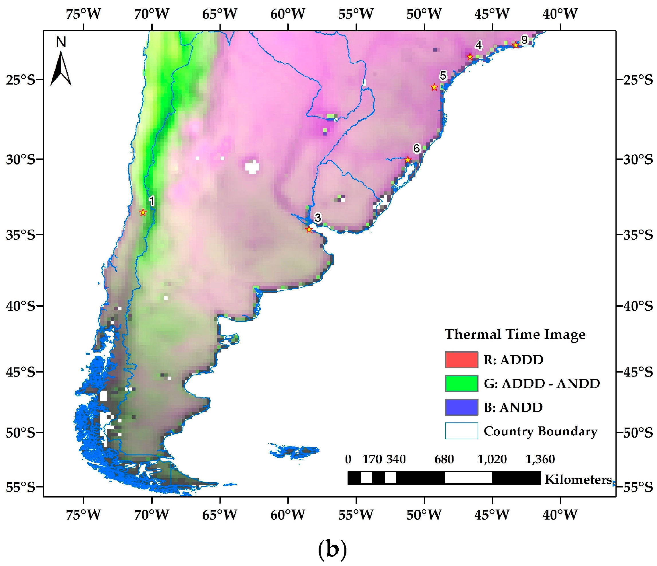
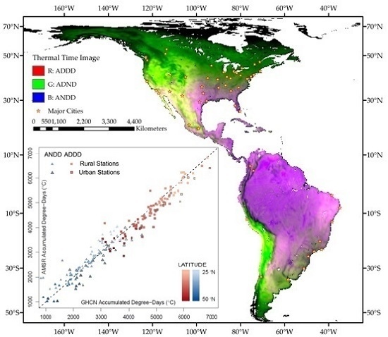
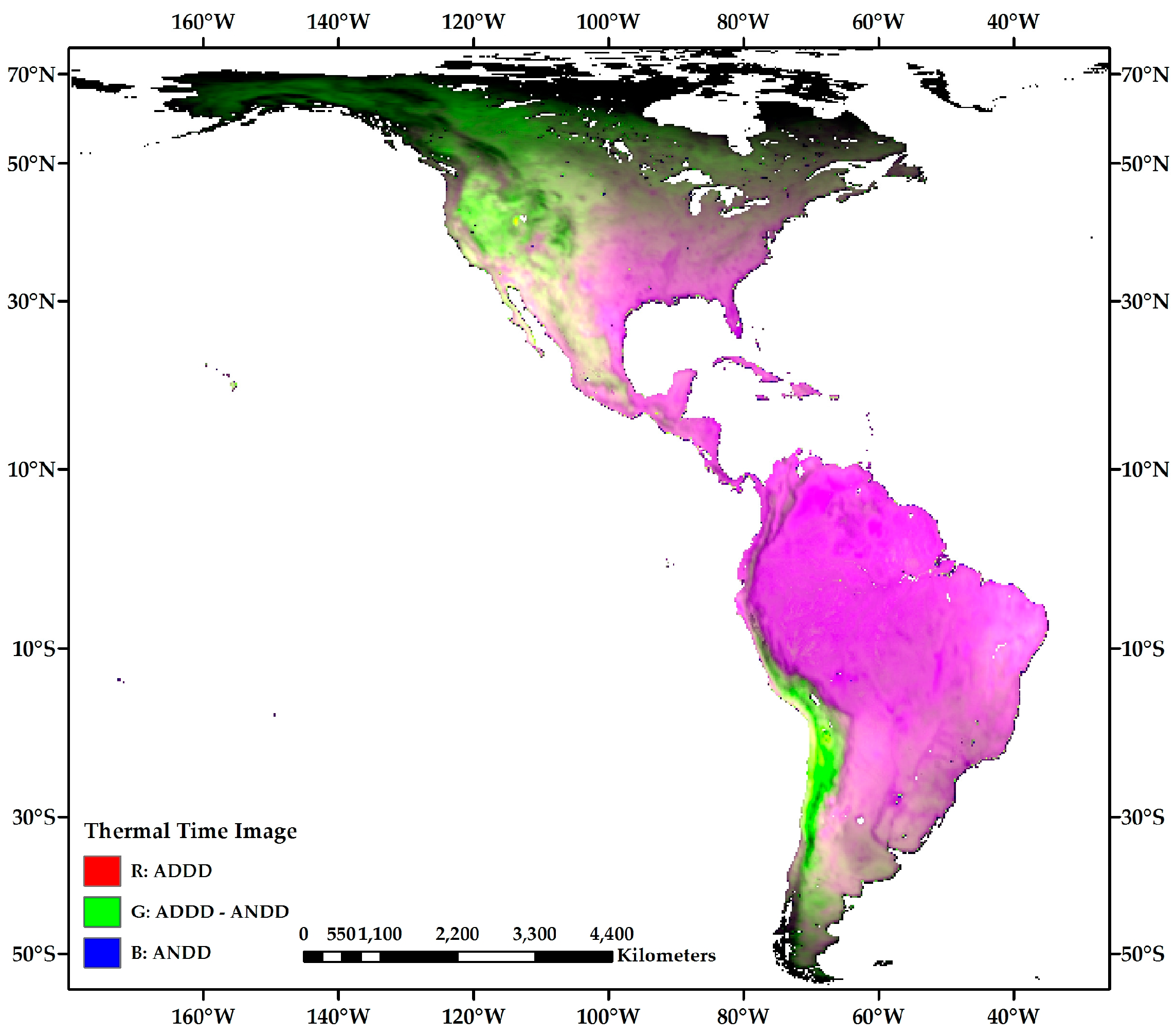
In the false color composite of accumulated thermal time metrics over the Western Hemisphere (Figure 1), areas shaded in green have low values of both ADDD (red) and ANDD (blue), but high values of Average day-night differences (ADND) (green). In other words, day-night thermal variation of those green pixels is very high as a proportion of the sum of daytime and nighttime heat. In contrast, red-purple pixels are areas with limited variation in day-night thermal range. Along coastlines and shorelines, the retrieval of air temperature sometimes failed, which resulted in a speckling of green or black pixels at the land’s edge.

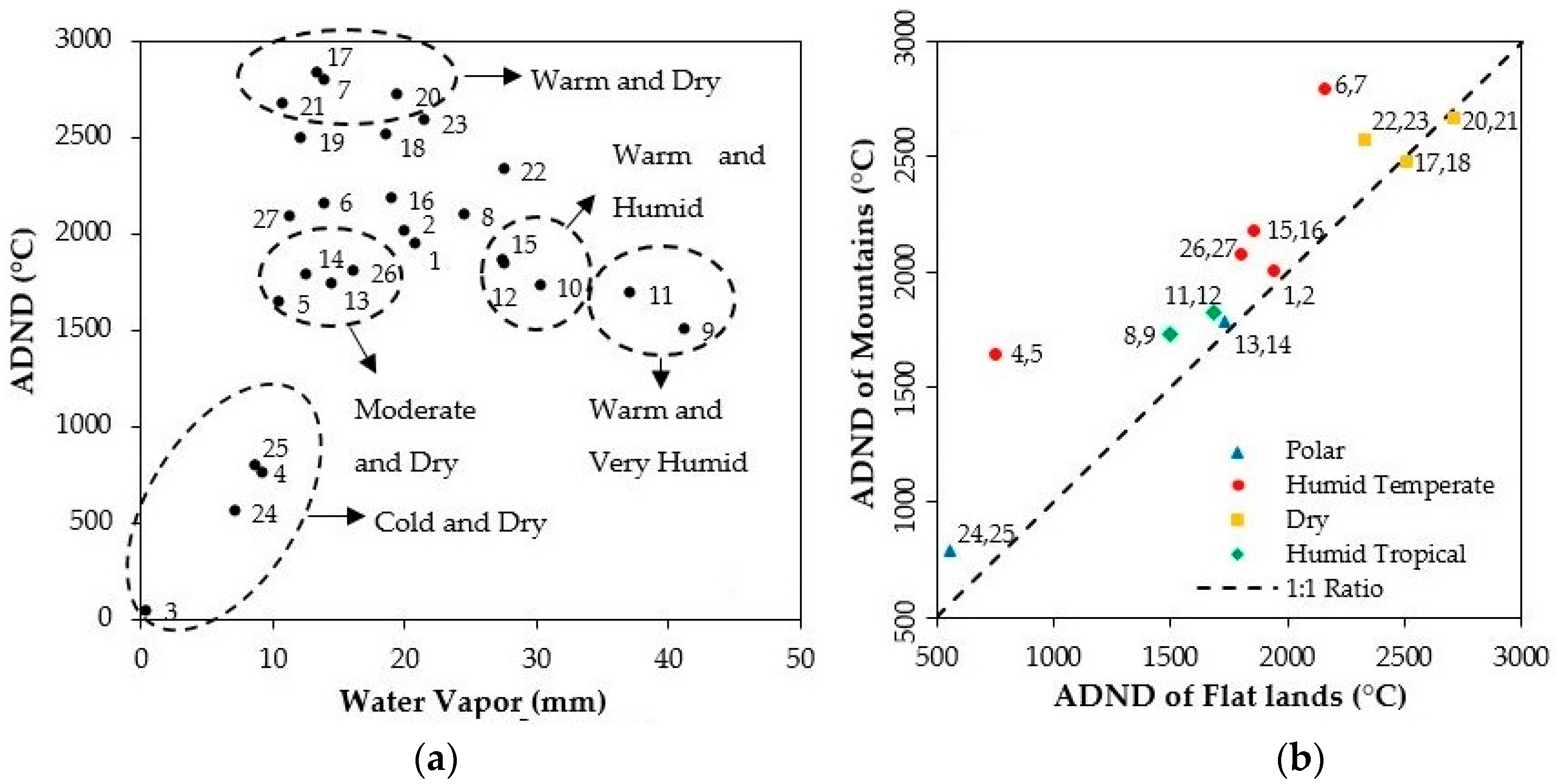
Latitudinal effects, water vapor (from multi-year daily average values [16,25]), and elevation generate different thermal regimes across continents. While the total heat available to an area is highly dependent on its latitude, the amount of atmospheric water vapor and elevation interact largely to control the day-night (or diel) thermal range. High latitude lands (above 50°N and 50°S), including tundra and polar regions, receive many hours of insolation over the growing season, but the total heat is still much lower than regions at lower latitudes (Figure 2a); thus, the shades are darker green, indicating that the diel variation is larger as a proportion of the total heat (Figure 1). In contrast, warm and dry ecoregions have the highest day-night thermal difference (Figure 2a). Note, for example, the bright green shades of Basin and Range province in the western United States or the Atacama Desert in western South America (Figure 1). Rainforest and savanna (Cerrado) regions of South America are the warmer and more humid regions in the Western Hemisphere and, thus, day-night differences are low, despite the high heat available, resulting in the shades of magenta in Figure 1. High and dry mountains appear darker relative to the neighboring lowlands, whether in the high Andes or the Canadian Rockies. A comparison between mountain areas and the lower elevations in similar ecoregions shows higher diel ranges at higher elevation as all data points in the Figure 2b are located above the 1:1 line.

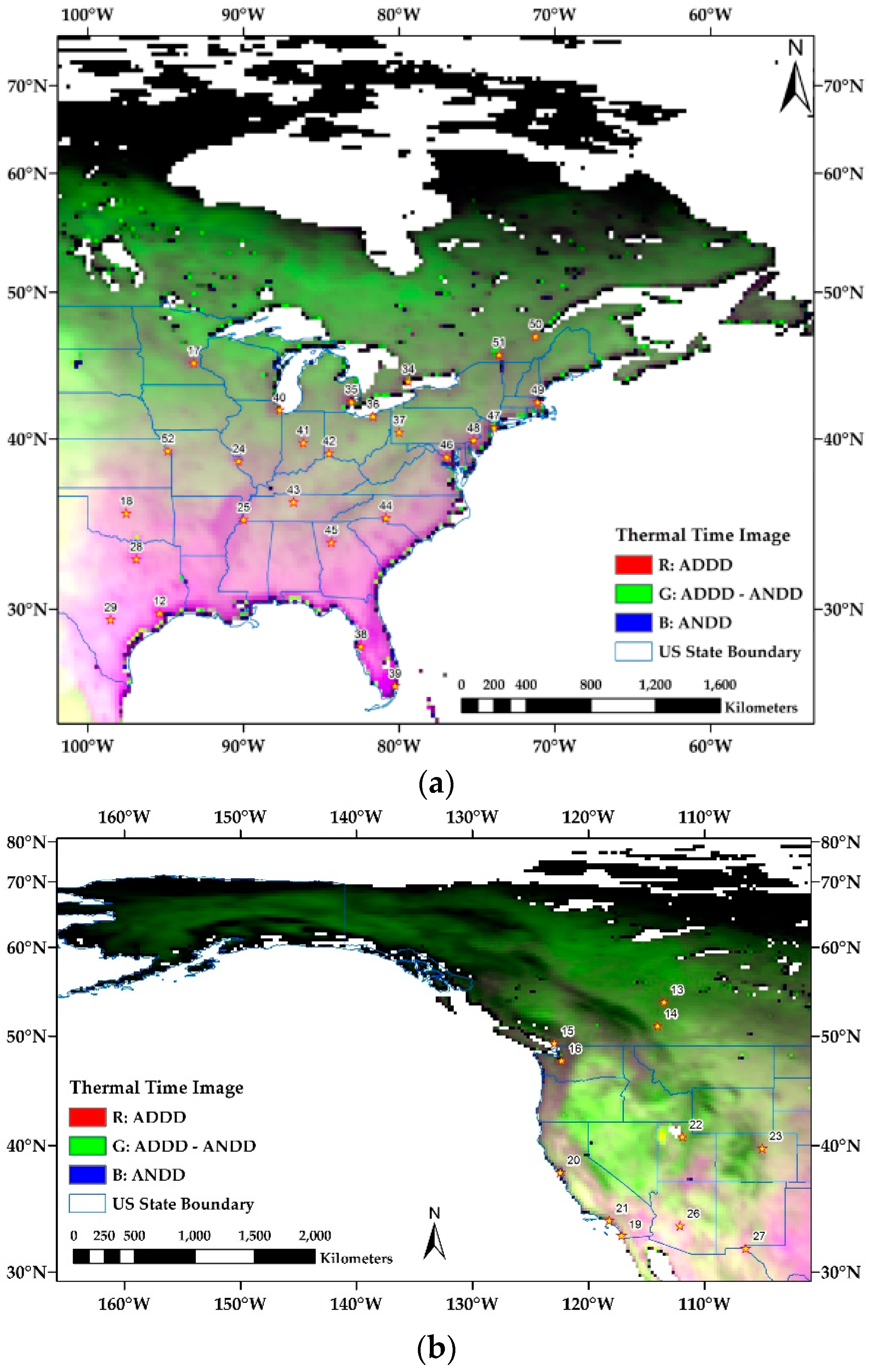
3.2. Urban Heat Islands at Regional Scale

Major inland cities of central and eastern USA, such as Minneapolis-St Paul (MN), Dallas-Fort Worth (TX), Atlanta (GA), St Louis (MO), Nashville (TN), Indianapolis (IN), and Cincinnati (OH), appear as small magenta blooms on the image, which indicates their lower day-night differences compared to that of adjacent rural areas (Figure 3). The air temperature data for major coastal urban agglomerations, such as the northeast corridor from Boston to Washington, Miami (FL), Houston (TX), Chicago (IL), and Detroit (MI), are all affected by adjacent open water leading to missing observations near the shorelines. Urban pixels located farther inland, however, do show lower ADND compared to surrounding rural areas (Figure 3). The two largest cities in Florida—Miami and Tampa—are not clearly distinguishable from the surrounding watery environment. It is also difficult to observe the UHI effect in the cities along the Pacific Coast.

UHI effects are evident with inland cities. Although Phoenix-Tucson (AZ) and El Paso (TX) are located in ecoregions with high average ADND (22 and 20, respectively, in Figure 2a), the two urban areas both have lower thermal day-night variation than surrounding areas as indicated by the light shades of magenta (Figure 3b). While El Paso is a part of the green belt along the Rio Grande River, we attribute the lower day-night thermal variation of Phoenix-Tucson to the extensive use of irrigation to maintain vegetated surfaces in and around Phoenix (and to a much lesser extent in Tucson). Salt Lake City and Denver are both located at higher, drier elevations resulting in higher ADND. Although both cities appear slightly darker than nearby pixels, the differences are not sharp, likely due to the spatial resolution of the AMSR grid being too coarse to capture the rapid spatial changes from rough terrain.

In central Canada, major cities are located nearby large water bodies; thereby generating missing observations (Figure 3a). However, we are still able to observe UHI effects in those cities as indicated by the dark magenta of inland urban pixels compared to the green shade of adjacent rural areas. Major cities in western Canada, including Vancouver, Edmonton, and Calgary (Figure 3b), are small in extent. While “error pixels” cover Vancouver entirely, the other two cities appear to have a slightly lower thermal variation as indicated by slightly darker green shade in the cities. However, since Edmonton and Calgary are both located at high latitudes where the regional thermal budgets and day-night thermal differences are already low, contrasts between urban and rural areas are weaker.

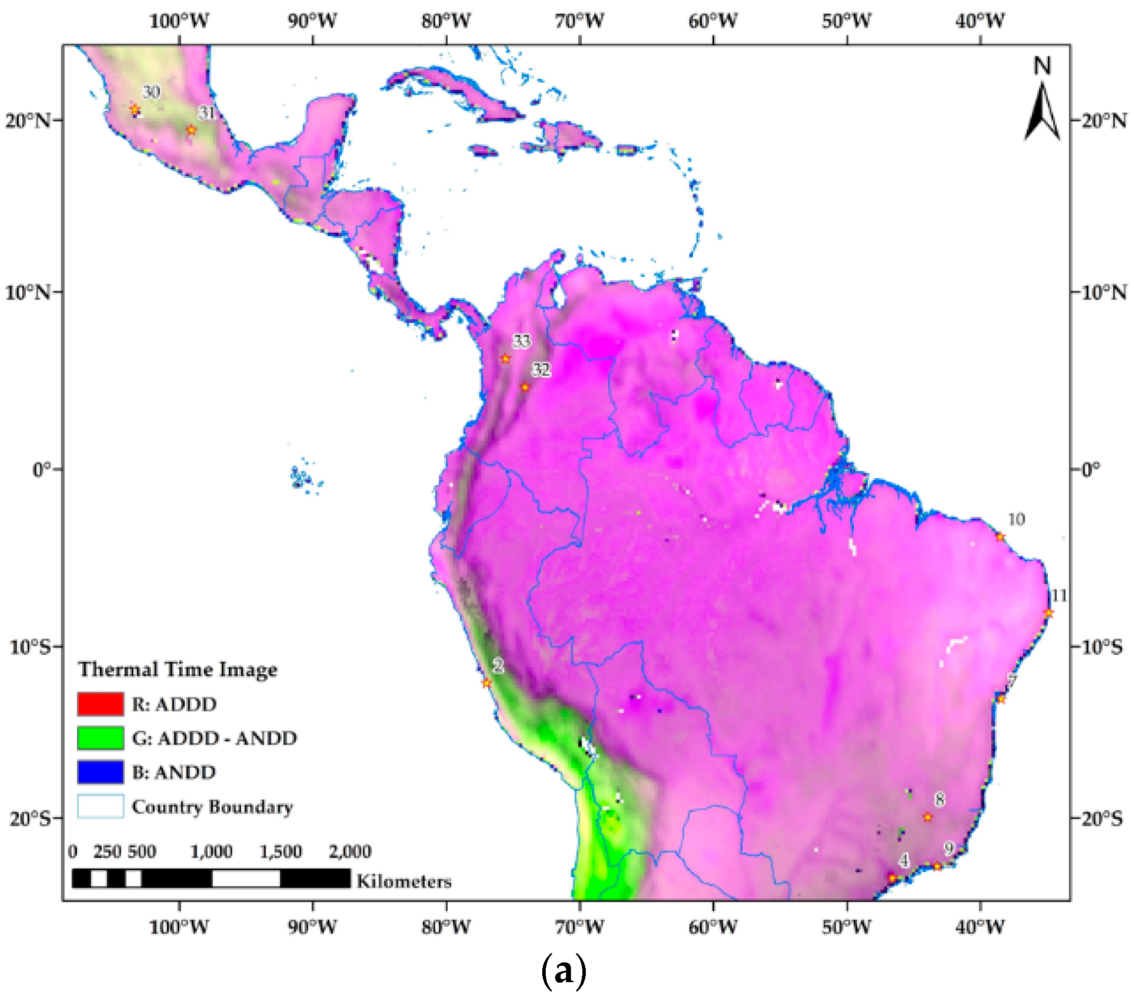
Guadalajara and Mexico City are the two largest cities in Mexico, and both are located on the Mexican Altiplano. In Guadalajara, there is no difference in the thermal pattern between urban and rural areas, possibly due to its small spatial extent. Mexico City is the only city in tropical America to exhibit clear differences between urban and rural thermal times (Figure 4a). Total day-night difference of Mexico City appears slightly weaker than surrounding lands as indicated by a darker shade. Major cities in the Andes Mountains region (Figure 4), including Medellin and Bogota (Colombia), Lima (Peru), and Santiago (Chile) are highly populated but small in extent. In addition, they are either located in rough terrain or on the coast. We cannot see UHI effects in those cities at the coarse spatial resolution of the microwave data.

Most of the major cities in Brazil are located on the coast, including Fortaleza, Recife, Salvador, Rio de Janeiro, and Porto Alegre (Figure 4). Due to their small extents, most of Brazil’s coastal cities are covered by error pixels. We do not see any influence of those cities on the thermal budget of inland pixels as was seen in the eastern US. Although São Paolo and Curitiba are both located farther inland, they demonstrate very different thermal dynamics. While Curitiba does not exhibit UHI effect, total day-night thermal variation is very strong in São Paolo, as indicated by a much darker magenta shade in the city compared to adjacent rural areas. In Belo Horizonte, the only major interior city, thermal difference between urban and rural is very low, likely due to terrain effects. Buenos Aires, the major city in Argentina, is an oddity: its day-night variation is higher in the city than in the surrounding rural areas in stark contrast to the other major cities in the Western Hemisphere.

3.3. Urban Heat Islands: A Comparison between Ground Observations and Remotely Sensed Data

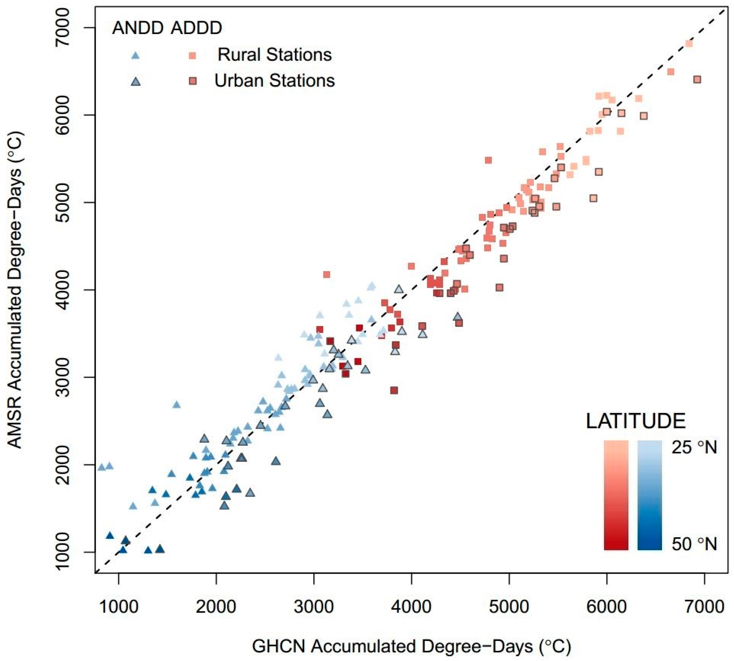
In this section, we zoom in from the subcontinent scale to individual cities. Figure 5 shows multi-year average ADDD and ANDD estimated from GHCN and AMSR surface air temperature data (values are provided in Table S2). The ADDDs from the microwave data are lower than station observations, as shown by the majority of ADDD data points being located below the 1:1 line. GHCN ADDDs are higher than values estimated by AMSR in both urban and rural areas by an average of 8.4% and 1.8%, respectively. The higher ADDD difference in cities indicates stronger urban effect in ground observations than in satellite-based temperature retrievals. In contrast, rural ANDD seems to be comparable between the two datasets as data points are equally distributed around the 1:1 line. However, AMSR urban ANDD are clearly lower than GHCN urban ANDD. Latitudinal effects on thermal time are evident in both datasets, indicated by a gradual decrease in thermal time metrics: moving northward from 20° to 50° north, ADDD decreases from 7000 °C to 3000 °C and ANDD decreases from 4000 °C to 1000 °C.

Over the 27 areas, we compare accumulated diurnal and nocturnal degree-days for 83 urban-rural pairs. ADDD estimated from AMSR data tends to be lower in cities than in adjacent rural areas, with only 15 of 83 pairs showing higher ADDD values in urban areas. Average ADDD and ANDD from AMSR data are lower in cities than adjacent rural areas by 4.2% and 2.1%, respectively. However, in the pairwise comparison, ANDD is higher in urban compared to rural areas 55.4% of the time (46/83). On the other hand, ADDD and ANDD estimated from GHCN data show consistently higher thermal time metrics in cities compared to surrounding rural areas: 81.9% of ADDD and 92.8% of ANDD show higher values in cities. Moreover, the average ADDD and ANDD are higher in cities than paired rural areas by 2% and 14.2%, respectively. GHCN data clearly show a pronounced UHI effect at night.

Large water bodies pose significant impacts on both day and nighttime temperature retrievals from AMSR. Average ADDD and ANDD estimated from GHCN sites located inside the seven coastal cities (Chicago, Toronto, Seattle, Washington, DC, New York, Montreal, Detroit) are higher than similar calculations using AMSR data by 16.5% and 20.6%, respectively; whereas, differences at rural sites that are located farther inland are within 5% for both daytime and nighttime measurements.

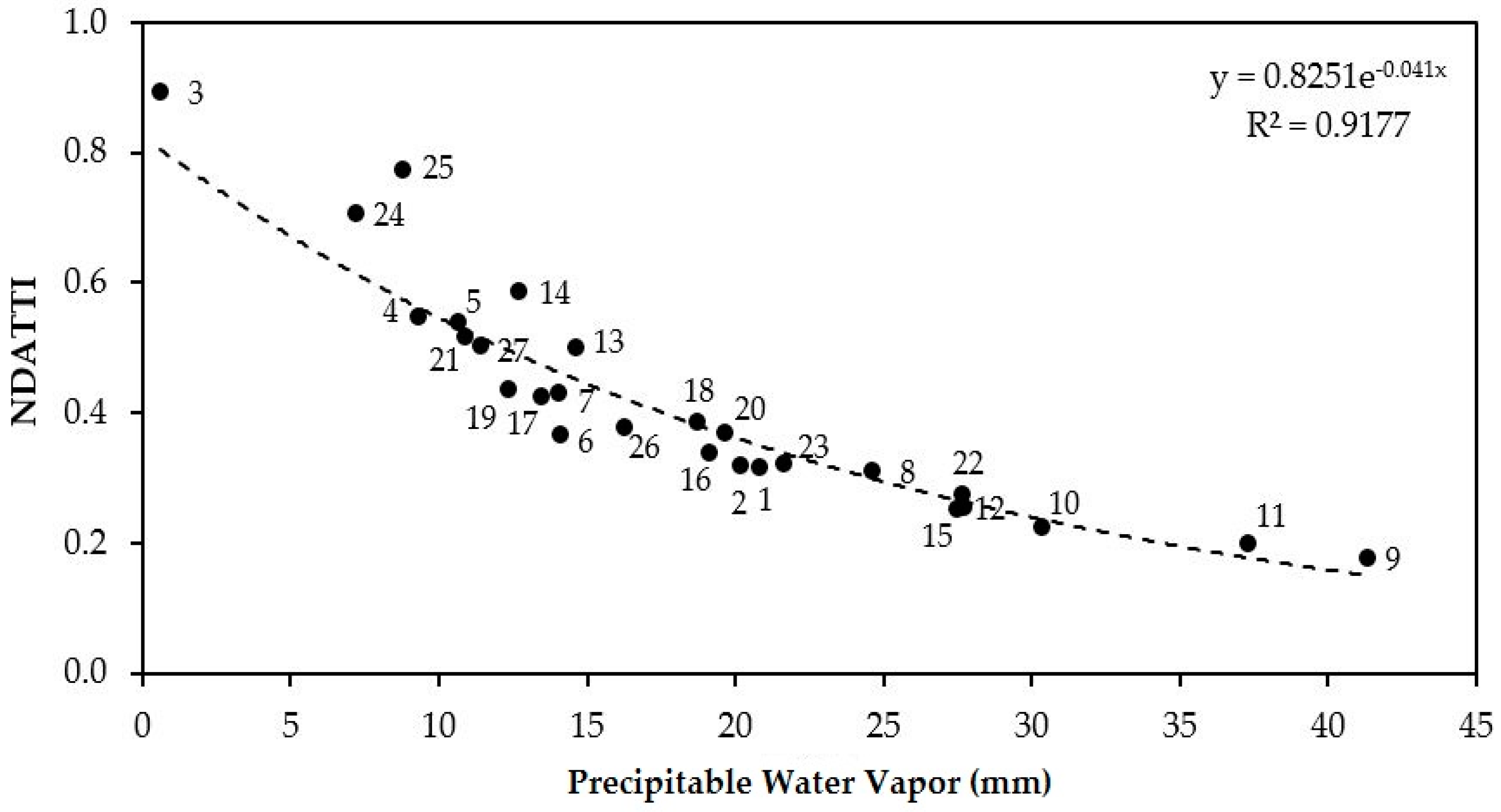
Figure 1 suggests that accumulated day-night differences in thermal time (ADND) are a better indicator for different land surfaces than either daytime or nighttime thermal time metrics alone. However, ADND is impacted by both water vapor and latitude (Figure 2a). Thus, we propose the NDATTI (Equation (6)) as an alternative to ADND through control of the effect of latitude. There is a strong relationship between NDATTI and water vapor (Figure 6). Ecoregions with drier climates have higher NDATTI values, and more humid regions have lower values of NDATTI. Compared to ADND, NDATTI attenuates the latitudinal effect so that water vapor is the key factor. NDATTI estimated for 83 urban-rural pairs from both AMSR and GHCN dataset show consistently lower values in urban areas than surrounding rural areas for more than 90% of comparisons in both datasets.

4. Discussion

Estimated accumulated nocturnal degree-days (ANDD) from AMSR and GHCN surface air temperature agree with previous findings that urban heat island effect is more pronounced at night [7,10]. However, accumulated diurnal degree-days estimated by AMSR data in major cities across the Western Hemisphere appear to be lower than surrounding rural areas (Section 3.3), with the only exception being in Buenos Aires, Argentina (Figure 4). We attribute that pattern partly to a large spatial extent of microwave observations resulting in heterogeneous pixels that include much more than just urban impervious surfaces. Temperature measurements from weather stations represent the conditions of a limited area around the site. On the other hand, surface air temperature retrieved from the AMSR data nominally cover 625 km². Urban land uses captured in coarse pixels may include developed lands, green spaces, water bodies, and the urban-suburban-exurban gradient around the city proper. This classic geographical problem of comparing point to areal measurements does not have a ready solution, but the key conclusion from our results is that the passive microwave measurements have the possibility of retrieving UHI effects. Although the coarse spatial resolution is not appropriate for studying particular cities, it holds promise for monitoring the effect of urbanized surfaces at regional to continental scales and possibly linking with meteorological and climatological simulation models.

Despite the advantage of “seeing” through the clouds and at night, surface air temperature data retrieved from microwave radiometers suffers some limitations in addition to the spatial resolution challenge. First, observations are only available over land; thus, cities with extensive shorelines may not be well imaged. Second, over areas with significant relief, the actual surface area contributing to the observed flux is larger than the nominal area leading to potential biases. Third, observations are limited to the frost-free period. Fourth, despite the recent production of a dataset spanning more than a decade, the observational record remains much shorter than comparable land surface temperature datasets generated from thermal infrared sensors.

It can be argued that the comparison between AMSR and GHCN surface air temperature data is inappropriate due to the scale disparity. Our results do suggest that ADDD in urban areas seem to be underestimated by the AMSR data (Figure 5). While urban temperatures estimated by ground observations are consistently higher during both daytime and nighttime, microwave-based ADDD in urban areas tends to be lower than in adjacent rural areas (Section 3.3). Despite differences in spatial resolution and the physical process behind the GHCN and AMSR data, the NDATTI estimated from both datasets are consistently lower in urban areas. This result suggests that NDATTI could be a better way to examine and compare UHIs from multiple data sources. In the rapidly urbanizing world, cross-comparison between various datasets will allow us to characterize and eventually model UHI effects more accurately. The major limitation with the NDATTI is that its calculation requires consistent temperature observations over a long period, which remains a challenge for many parts of the world. For example, we were not able to select any urban-rural pairs in South America that met our screening criteria to calculate thermal time metrics.

5. Conclusions

Urban heat islands have been long studied using both ground-based observations and TIR remotely sensed data. While observation-based studies are limited to regional scales or beyond, satellite-based UHI studies using TIR time series are often limited by low temporal resolution in many parts of the world. Our study takes advantages of passive microwave data to study UHI effects at regional to continental scales. We used the two measurements of thermal time metrics, ADDD and ANDD, to characterize the heat accumulation in urban and surrounding rural areas during the warm period between the equinoxes. We also proposed a new index, the normalized difference accumulated thermal time index or NDATTI, to examine and compare urban heat islands across latitudes. Our results indicate that day-night thermal variations, as well as NDATTI values, are lower in urban than adjacent rural areas. To better demonstrate the capability of AMSR near-surface air temperatures in the urban study, we compare that dataset to station observations from the Global Historical Climate Network for 27 major cities in the North America. The consistently lower urban NDATTI than rural values in both datasets suggest that our proposed index could prove useful for comparative UHI studies using multiple data sources.