Article

Estimating the Total Nitrogen Concentration of Reed Canopy with Hyperspectral Measurements Considering a Non-Uniform Vertical Nitrogen Distribution

1
Key Laboratory of Watershed Geographic Sciences, Nanjing Institute of Geography and Limnology, Chinese Academy of Sciences, Nanjing 210008, China
2
School of Earth Sciences and Engineering, Hohai University, Nanjing 210098, China
*
Author to whom correspondence should be addressed.
Remote Sens. 2016, 8(10), 789; https://doi.org/10.3390/rs8100789
Submission received: 12 May 2016 / Revised: 25 August 2016 / Accepted: 19 September 2016 / Published: 23 September 2016
(This article belongs to the Special Issue What can Remote Sensing Do for the Conservation of Wetlands?)

Abstract

:
The total nitrogen concentration (NC, g/100 g) of wetland plants is an important parameter to estimate the wetland health status and to calculate the nitrogen storage of wetland plants. Remote sensing has been widely used to estimate biophysical, physiological, and biochemical parameters of plants. However, current studies place little emphasis on NC estimations by only taking nitrogen’s vertical distribution into consideration, resulting in limited accuracy and decreased practical value of the results. The main goal of this study is to develop a model, considering a non-uniform vertical nitrogen distribution to estimate the total NC of the reed canopy, which is one of the wetland’s dominant species, using hyperspectral data. Sixty quadrats were selected and measured based on an experimental design that considered vertical layer divisions within the reed canopy. Using the measured NCs of different leaf layers and corresponding spectra from the quadrats, the results indicated that the vertical distribution law of the NC was distinct, presenting an initial increase and subsequent decrease from the top layer to the bottom layer. The spectral indices MCARI/MTVI2, TCARI/OSAVI, MMTCI, DCNI, and PPR/NDVI had high R2 values when related to NC (R2 > 0.5) and low R2 when related to LAI (R2 < 0.2) and could minimize the influence of LAI and increase the sensitivity to changes in NC of the reed canopy. The relative variation rates (Rv, %) of these spectral indices, calculated from each quadrat, also indicated that the top three layers of the reed canopy were an effective depth to estimate NCs using hyperspectral data. A model was developed to estimate the total NC of the whole reed canopy based on PPR/DNVI with R2 = 0.88 and RMSE = 0.37%. The model, which considered the vertical distribution patterns of the NC and the effective canopy layers, has demonstrated great potential to estimate the total NC of the whole reed canopy.

Graphical Abstract

1. Introduction

Nitrogen is one of the elements triggering the eutrophication of wetlands, which ultimately leads to wetland degradation. Nitrogen is also a necessary element for wetland plant growth and development [1]. Wetland plants can remove nitrogen from the wetland environment by absorbing nitrogen for their growth and development, which is the theoretical basis of wetland restoration by means of cultivated plants [2,3,4]. Estimation and dynamic monitoring of nitrogen concentrations and nitrogen storage (biomass × nitrogen concentration) of wetland plants are critical for wetland evaluation and management, providing important information for adjusting and optimizing wetland management strategies and for improving and evaluating wetland quality and health.
Nitrogen measurements based on destructive point sampling and laboratory methods, despite being effective and accurate, are laborious and time-consuming and thus fail in quickly capturing nitrogen concentrations both temporally and spatially at regional scales [5]. Remote sensing data, including hyperspectral optical/thermal and synthetic aperture radar (SAR) and satellite data, enables timely and nondestructive plant status assessment and is widely used, becoming increasingly important for large-area estimations of biophysical, physiological, and biochemical plant parameters, such as leaf area index (LAI), above-ground biomass, leaf and canopy chlorophyll content, nitrogen concentration (NC, g/100 g) and canopy water content [5,6,7,8,9,10,11]. Many studies have focused on agricultural crops—including wheat, rice, corn, and cotton—and the types of forest vegetation [12,13,14,15]. However, little attention has been paid to estimating NC of wetland plants with the remote sensing technique.
Various methods have been developed to estimate and map plant canopy nitrogen status, including NC and nitrogen content, using hyperspectral reflectance information [16,17,18]. However, the methods rarely take the non-uniformity of nitrogen distribution into consideration. According to the light distribution patterns within a canopy, optimization theory suggests that plants should tend to allocate more nitrogen to the upper levels of the plant canopy than its lower level in an effort to maximize total canopy photosynthesis because the upper canopy leaves are exposed to better light conditions than the lower shaded leaves [19,20]. This theory implies that the distribution of leaf nitrogen in plants of a canopy is non-uniform, and this theory is further supported by a series of studies, indicating that the vertical distribution of NC in a plant canopy is non-uniform [21,22,23,24]. Spectral reflectance of green vegetation within a range from 400 nm to 760 nm is primarily controlled by plant pigments. Given the pigments absorb most of the incident radiation in the 400–760 nm range, the canopy’s spectral reflectance of green vegetation in this range is mainly affected by the upper leaf layers [25]. However, it is still unclear which leaf layers in the canopy should be involved in building a remote sensing-based model for estimating NC. Consequently, the determination of canopy NC based on canopy spectral reflectance, without considering the non-uniform vertical nitrogen distribution, would lead to low accuracy in estimating canopy NC [18,23].
The NC and nitrogen storage of different wetland plants are distinct due to their different nitrogen uptake capacities [26]. Reed, Phragmites australis, is a dominant wetland species, accounting for approximately 40% of a wetland’s ecological community [27,28]. It is the most frequently used plant species worldwide in constructing wetlands for wastewater treatment and wetland restoration because of its high biomass production and ability to uptake nitrogen, and it is also an important nitrogen sink in eutrophic lakesides, littoral zones, and along rivers and marsh wetland [3,29,30]. Therefore, the objectives of this study include (1) roughly identifying vertical distribution patterns in the NC of a reed canopy; (2) determining the effective leaf layers for estimating NC of reed canopy using hyperspectral remote sensing data; and (3) establishing a remotely sensed model for estimating the total NC of the whole reed canopy accounting for the vertical distribution patterns of NC and the effective canopy layer.

2. Materials and Methods

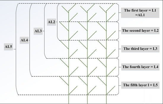
2.1. Field Experiments

Experiments were carried out in three different fields. Experiment I was conducted on 22–24 June 2014, at the lakeside of the Hongze Lake wetland (33.23131°N, 118.30698°E) in Jiangsu province. Experiment II was conducted on 11–14 July 2014, at the bank wetland of the Yangzi River (32.12353°N, 118.7369°E) in Jiangsu province. Experiment III was conducted on 21–25 July 2014, at the Poyang lake wetland (29.45151°N, 116.06231°E) in Jiangxi province. A total of 60 representative quadrats, each with a size of 1 m × 1 m, were selected and measured, including 15 quadrats from Experiment I, 22 from Experiment II, and 23 from Experiment III.
The measured reed beds of the three experiment fields have the same sediment conditions, that is, marshy soil without the water column. An early study indicated that there was a large temporal variation in the reed bed spectra, and the optimal time for data acquisition differed for old reed beds and new ones [31]. New reed beds are characterized by no dead stems and new, live stems reproduced, whereas the old reed beds have erect, dead stems and new, live stems emerging amongst the dead stems. The three experimental fields all contained new reed beds. The reed beds were all in the peak growing stage without flowering during the experimental periods. The average reed height of the quadrats ranges from 1.8 m to 2.5 m; the density ranges from 62 to 74 pcs/m2; and each plant has approximately 11–15 leaves.

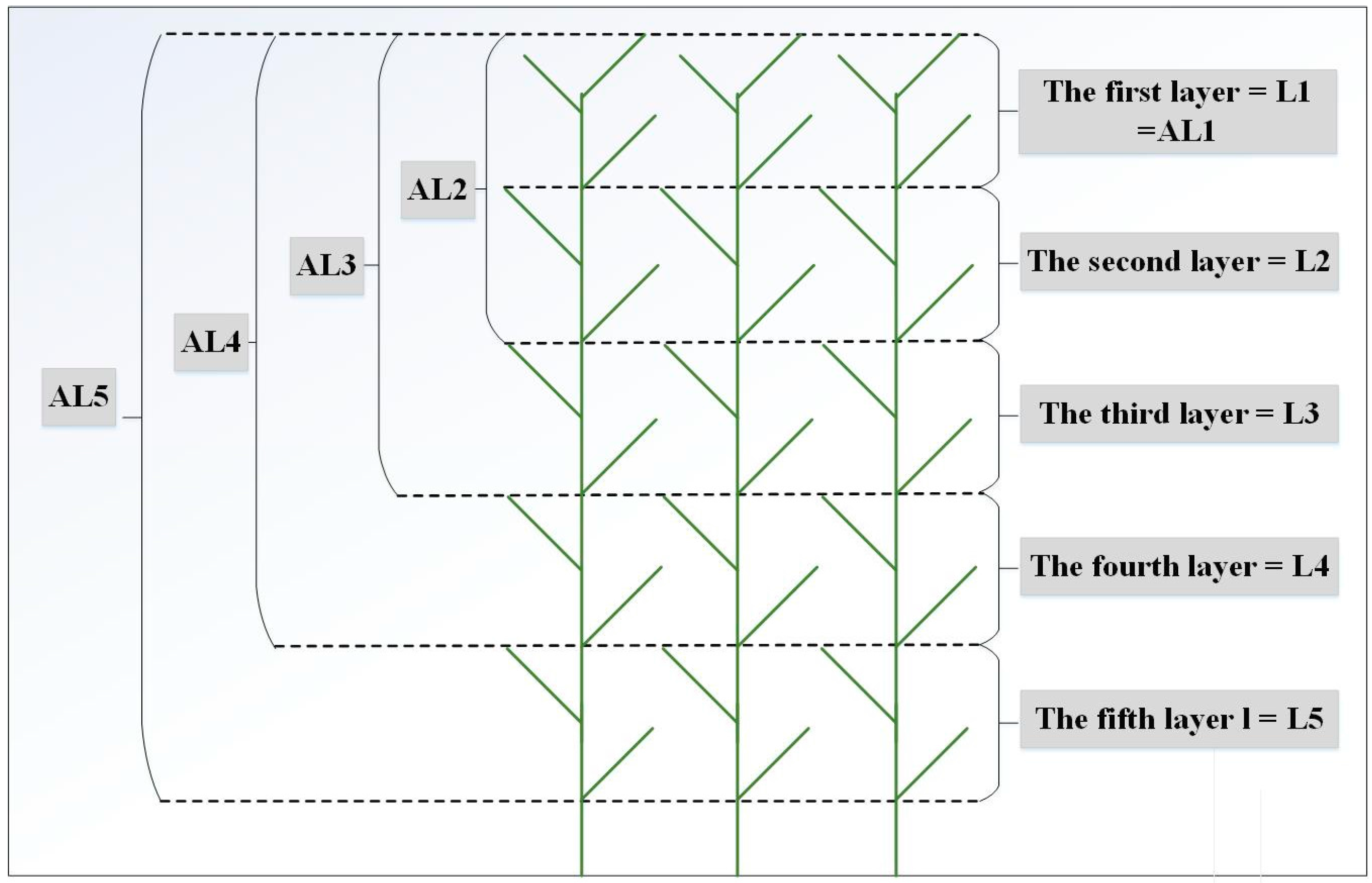
2.2. Experimental Design and Spectral Reflectance Measurement

Since the average reed height at peak growing stage is 1.8–2.5 m, we divided the reed canopy height into five equal layers by height from top (L1) to bottom (L5) for each quadrat (Figure 1). To study the contribution of the leaves to canopy reflectance in each layer, the scheme was used where leaves were removed layer by layer, as shown in Figure 1. By removing the leaves from L5 to L2 in order, we measured the canopy reflectance and corresponding LAI from AL5 to AL2, respectively.
In consideration of the reed height, we measured canopy reflectance using a 2 m long telescopic ladder. The LAI of each target layer was measured using an LAI-2000 Plant Canopy Analyzer (LI-COR Inc., Lincoln, NE, USA) with three replicates, and the three LAI values were averaged to represent the LAI of the target layer. Canopy reflectance measurements were taken at a height of 1 m above the canopy using an ASD FieldSpec Pro spectrometer (Analytical Spectral Devices, Boulder, CO, USA) under clear, blue-sky conditions between 10:00 and 14:00 (Beijing Local Time). The spectrometer has a spectral range of 350–2500 nm and a field of view of 25°, and the spectral resolution (full width at half maximum, FWHM) was 3 nm for the 350–1050 nm region and 10 nm for the 1050–2500 nm region. The measured irradiance was converted to reflectance by recording the irradiance spectra from a 0.4 m × 0.4 m BaSO4 calibration panel. To reduce the possible effects of sky and field conditions, 20 repeated spectral measurements at each target layer of every quadrat were taken and averaged to represent the canopy reflectance of the target layer. Therefore, in every quadrat, five pairs of measurements from AL1 and AL5, including reflectance spectra and corresponding LAIs, could be obtained.
Two to three representative leaves of every layer in every quadrat were randomly selected as sample leaves, and the reflectance measurements (350–2500 nm) of these sample leaves were taken in the field using the ASD FieldSpec Pro spectrometer together with a leaf clip. ASD’s Leaf Clip assembly is designed specifically for use with the Plant Probe to simplify the process of collecting spectra on live vegetation. The unique design includes a gentle trigger lock/release gripping system for holding the target sample in place without removing the leaf from its habitat and inflicting damage. Five reflectance spectra were taken per leaf using an ASD leaf clip covering a halogen bulb-illuminated area with a radius totaling 10 mm. A mean reflectance spectrum was calculated for each sample leaf. Reflectance spectra of sample leaves in every layer were averaged as the leaf reflectance spectrum of the target layer.

2.3. Spectral Indices

Many studies have demonstrated that spectral reflectance of green plants in the spectral region of 400 to 800 nm is primarily governed by plant pigments (e.g., chlorophyll) that are absorbing most of the incident radiation, and some spectral vegetation indices (VIs) were developed based on spectral reflectance in the region to estimate the chlorophyll or nitrogen content of different plants [32]. However, previous research has shown that the spectral IVs tend to be sensitive to LAI [12,33]. To determine the effective leaf layers for NC estimation and estimate the total NC of the reed canopy using hyperspectral measurements, a spectral index that can minimize the influence of LAI and increase the sensitivity of changes in NC needs to be designed. Based on a literature review, 14 spectral VIs used to assess the chlorophyll or nitrogen content of different plants were selected to test their sensitivities to NCs and LAI of the reed canopy in this study (Table 1). The selected indices can be categorized into two types: 11 spectral VIs and 3 combined indices including MCARI/MTVI2, TCARI/OSAVI, and PPR/NDVI.

2.4. Nitrogen Concentration Measurements

After measuring reflectance, the leaves were sealed in a bag and sent to the laboratory for nitrogen concentration measurements via the Kjeldahl method, and the NCs from L1 to L5 in each reed quadrat were obtained. The NCs of AL1, AL2, AL3, AL4, and AL5 were calculated using the following formula:
N A L i = 1 i ( N L i ) / i
where i is the layer number with value i = 1, 2, 3, 4, 5; NALi is the NC (g/100 g) of ALi; and NLi is the NC (g/100 g) of Li.

2.5. Modeling and Validation of Datasets

We measured a total of 60 representative quadrats from all three experimental fields, including 15 quadrats from Experiment I, 22 quadrats from Experiment II, and 23 quadrats from Experiment III. According to the experimental design, each quadrat had five groups of data, including canopy spectra and corresponding NCs and LAIs from AL1 to AL5. We divided the 60 quadrats randomly into two parts: 40 calibration quadrats and 20 validation quadrats. The calibration quadrats contain 10 quadrats from Experiment I, 15 quadrats from Experiment II, and 15 quadrats from Experiment III. The canopy spectral data and corresponding NC from AL1 to AL5 measured in the 40 calibration quadrats are used to establish the model for estimating NC of reed, and the datasets of the validation quadrats were used to validate corresponding models.

3. Results

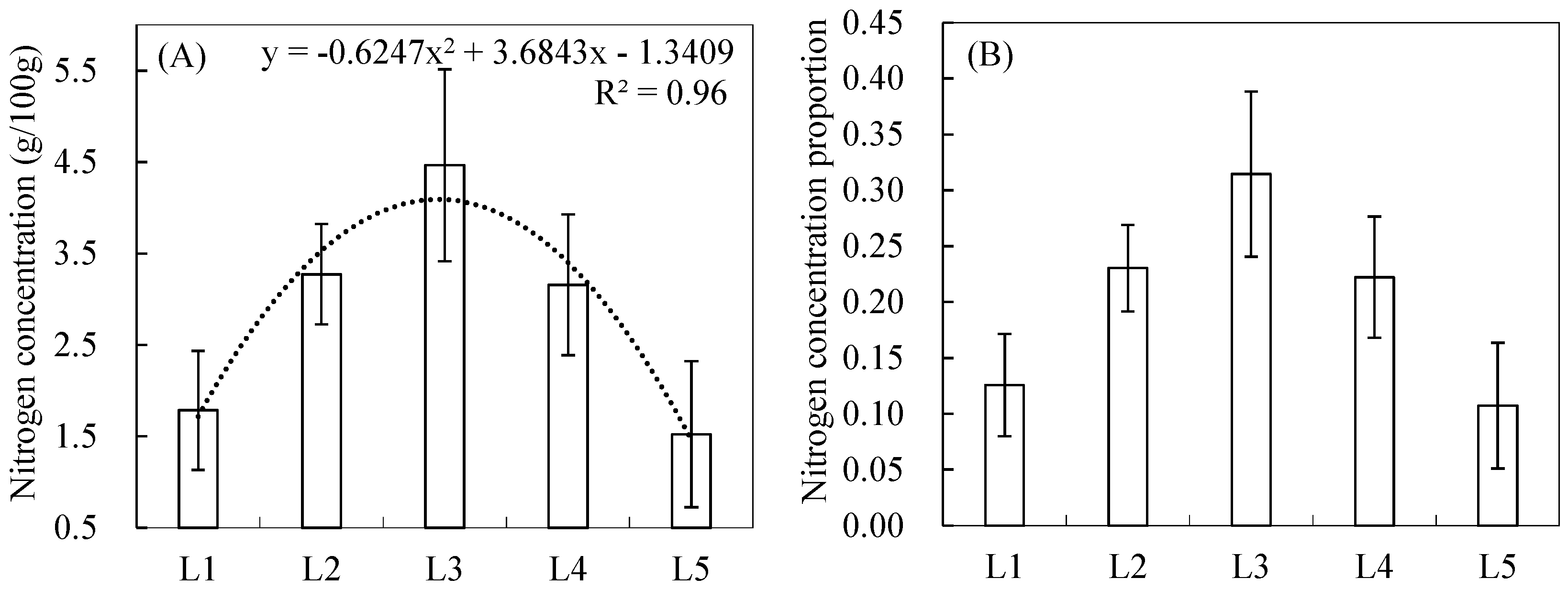
3.1. Vertical Distribution Pattern of Nitrogen Concentrations within the Reed Canopy

Figure 2A shows that the NC distribution of the leaf layers from the first layer (L1) to the fifth layer (L5) based on the leaf layer data from the 60 quadrats. The results demonstrate that the NCs of the leaf layers generally exhibited great vertical differences within reed canopies. From L1 to L5, the NC of the leaves initially increased and then decreased, with a quadratic curve (R2 = 0.96) (Figure 2A). The corresponding mean proportions from L1 to L5 were 0.13, 0.23, 0.31, 0.22, and 0.11, respectively (Figure 2B).

3.2. Estimation of Nitrogen Concentrations Using Spectral Indices

Figure 3 shows the mean reflectance spectra of the reed canopies from AL1 to AL5 of the 60 quadrats, which were recorded during successive leaf removals from L5 to L1. In Figure 3, small reflectance differences in the visible and short wave infrared regions could be observed between AL5, AL4, and AL3, and between AL2 and AL1, but only reflectance differences between AL3 and AL2 were statistically significant. The results suggest that the third layer (L3) is the key layer for reed canopy reflectance spectra and that AL3 has a great contribution to the reflectance in the visible and short wave infrared regions of the reed canopy, while AL2 also showed a significant contribution to the reflectance in the near infrared region.
Given the possible substrate influence on the spectra of AL1 and AL2, we analyzed only the canopy spectra measured from AL3 to AL5 of the quadrats, the corresponding NC and the LAI to test the relationship between LAI, NC, and spectral VIs (Table 2). The result shown in Table 2 indicate that the VIs were significantly related to LAI and NC (p < 0.01). The combined VIs MCARI/MTVI2, TCARI/OSAVI, and PPR/NDVI and the individual VIs MMTCI and DCNI were highly correlated with NC (R2 > 0.5) and had low R2 values when related to LAI (R2 < 0.2). Therefore, the five VIs could minimize the influence of LAI and increase the sensitivity to changes in NC. Of the indices, the PPR/NDVI produced the highest correlation with NC (R2 = 0.62) and the low correlation with LAI (R2 = 0.19) and was selected to estimate the total NC of the canopy reed.

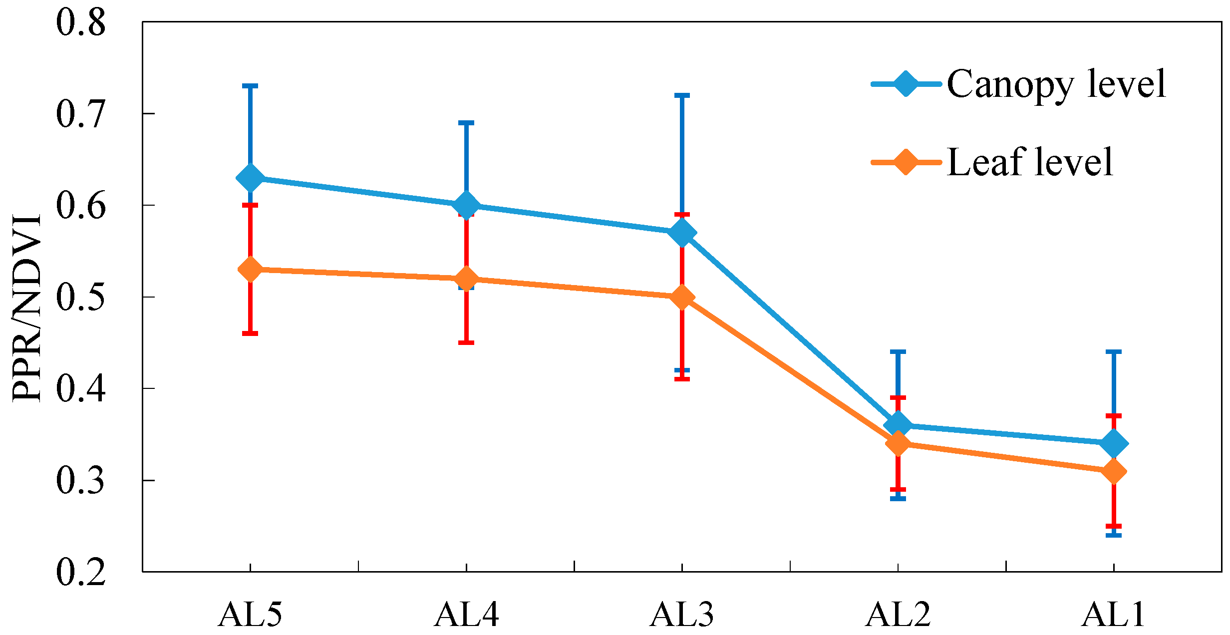
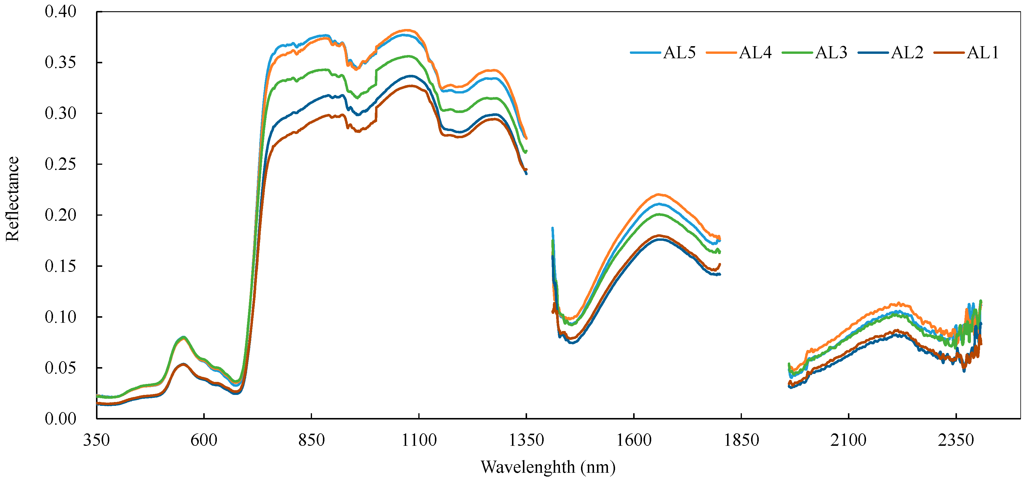
3.3. Variations in the Spectral Index for Different Layers of the Reed Canopies

In Table 2, the five VIs that have low sensitivity to the variation in LAI (R2 < 0.2) and high sensitivity to NC (R2 > 0.5) were further tested using a relative variation rate (RV, %). Rv, which was defined as the percentage difference of VIs between of ALi and ALi-1 divided by VI of ALi (i = 2, 3, 4, 5), was used to determine the change in magnitude of the VIs while removing layer leaves in order (Table 3). The results indicate that MMTCI and DCNI increase upon leaf removal from L5 to L1, whereas MCARI/MTVI2, TCARI/OSAVI, and PPR/NDVI decreased. Furthermore, for each VI, Rv was the highest when removing the leaves of the lower three layers, and of them, PPR/NDVI had the largest Rv value.
Since PPR/NDVI had the highest R2 with NC and the highest Rv (Table 2 and Table 3), we used PPR/NDVI to analyze the effective leaf layers for NC estimation at the canopy and leaf levels. The PPR/NDVI from AL1 to AL5 at the leaf level was calculated using the corresponding leaf reflectance, e.g., PPR/NDVI at leaf level of AL1 was calculated by averaging the leaf reflectance of the representative leaves of L1, and PPR/NDVI, at leaf level of ALi (i = 2, 3, 4, and 5), was calculated by averaging the leaf reflectance of all representative leaves from L1 to Li. In this way, we obtained PPR/NDVI values from AL1 to AL5 of each quadrat at the leaf level. At the canopy level, the PPR/NDVI from AL1 to AL5 for each quadrat was calculated using the canopy reflectance from AL1 to AL5. Figure 4 shows the PPR/NDVI variations from AL1 to AL5 at both the canopy and leaf levels. The results indicate that the variation of the PPR/NDVI was small when removing the leaves of L5 and L4, while the variation of the PPR/NDVI was the greatest when the leaves of L3 were removed. The variations in PPR/NDVI were consistent at the canopy and leaf levels. This suggested that the top three layers (AL3) may be an effective canopy for NC estimation using remote sensing data.

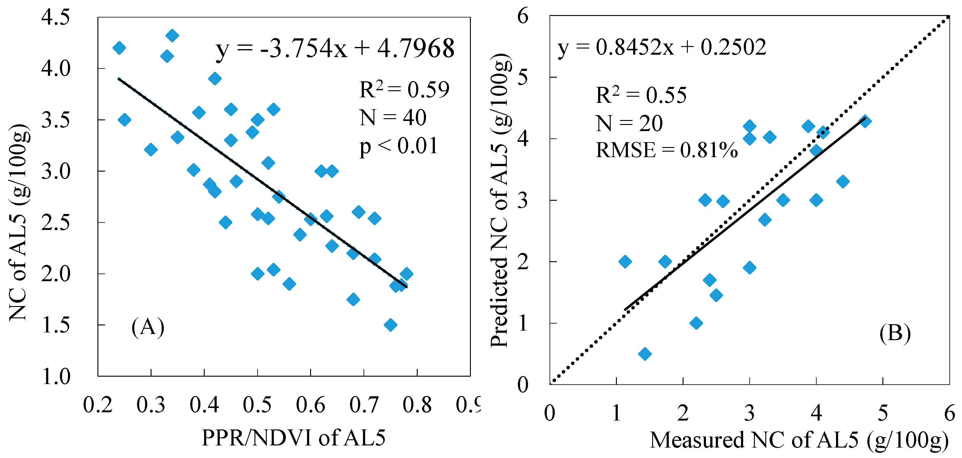
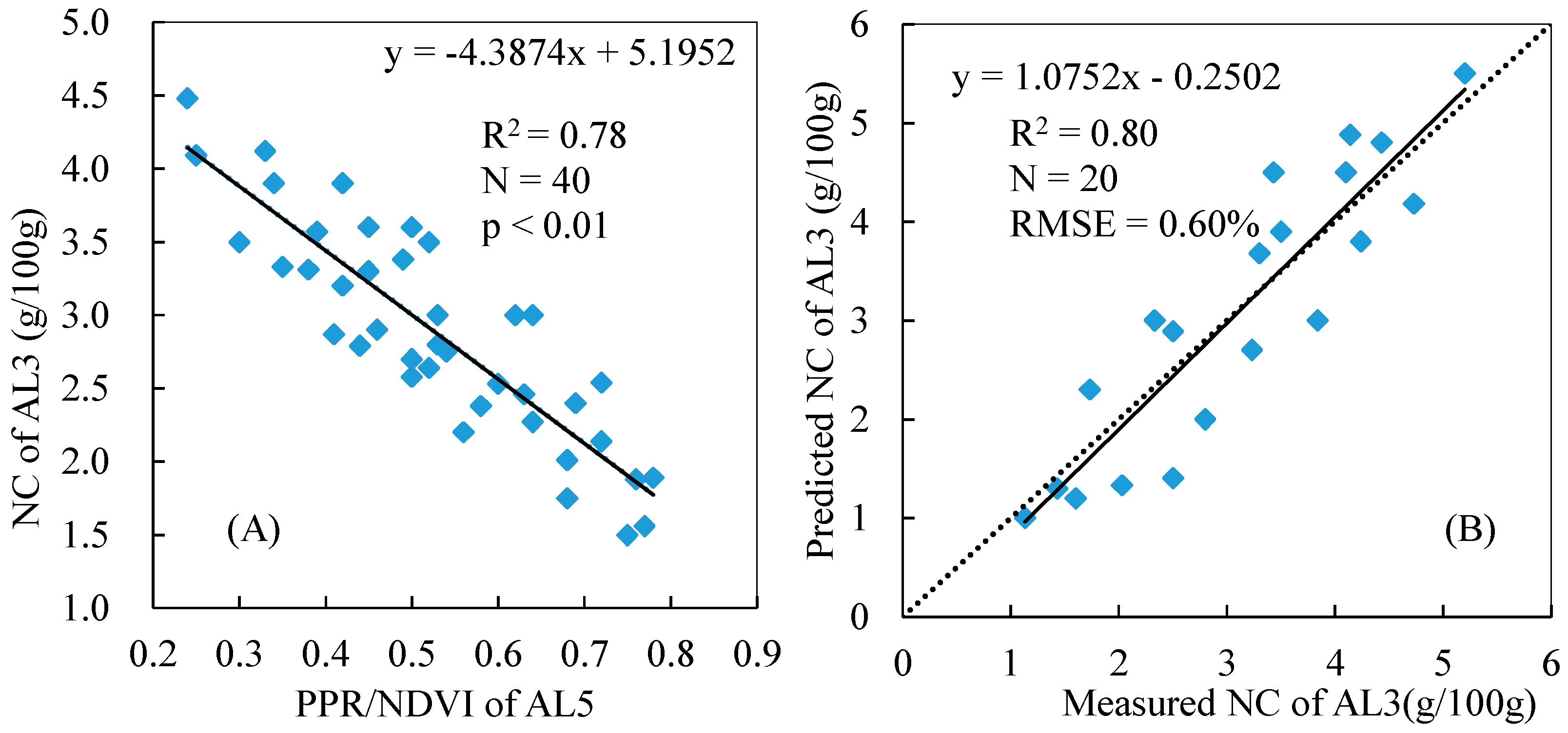
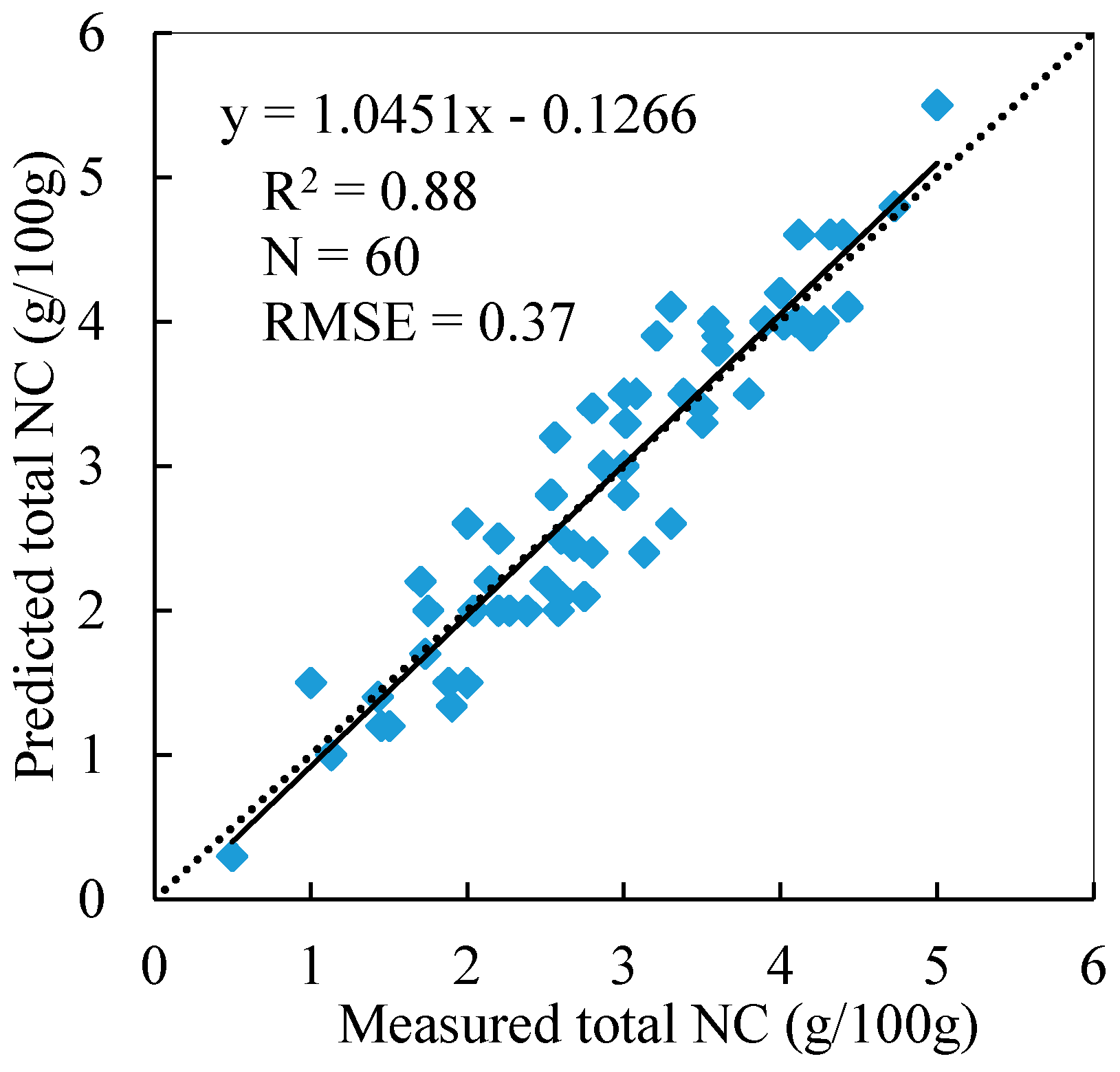
3.4. Total NC Estimation of Reed Canopies

Based on the results presented in Table 3, we selected PPR/NDVI to estimate the total NC of reed canopy because it has the highest R2 when related to NC. Figure 5A and Figure 6A show the relationships between the PPR/NDVI of AL5 and the NC of AL5 and between the PPR/NDVI of AL5 and the NC of AL3, respectively, based on the corresponding datasets of the calibration quadrats. The results indicate that there were better correlations between the PPR/NDVI of AL5 and the NC of AL3 (R2 = 0.78) than between the PPR/NDVI of AL5 and the NC (R2 = 0.59, Figure 5A). Figure 5B and Figure 6B show the validation results of the corresponding models based on the corresponding datasets of the validation quadrats. The result showed that the regression model (Y = −4.3874X + 5.1952) from Figure 5A used to estimate the NC of AL3 had a higher precision and robustness with R2 = 0.80 and RMSE = 0.60%. It could be concluded that the AL3 containing L1–L3 had greater potential than AL5 for predicting the total NC of the reed canopy using PPR/NDVI.
Based on the regression model to estimate the NC of AL3 (Figure 6A) and the vertical mean distribution proportion of NC within the reed canopy (Figure 2B), the model for estimating the total NC of the reed canopy was established as follows:
Yt = (−4.3874X + 5.1952)/(β1 + β2 + β3)
where Yt is the total NC of the reed canopy; X is PPR/NDVI of canopy level; β1, β2, and β3 are the mean NC proportions of L1, L2, and L3, respectively; and β1 = 0.13, β2 = 0.23, and β3 = 0.31 according to Figure 2B.
Using the PPR/NDVI values derived from the reflectance spectra of the 60 quadrats and Equation (2), the total NCs of the 60 reed quadrats were predicted and compared to the measured total NCs. The results show that the model performed well in estimating the total NCs of the reed canopy with R2 = 0.88 and RMSE = 0.37% (Figure 7).

4. Discussion

In this paper, we divided the reed canopy into five layers to obtain the vertical distribution patterns of the NC within the reed canopy based on remote sensing data. Our results indicate that NCs in the leaves of the reed canopy first increase and then decrease from L1 to L5, with the highest NC appearing in L3. Such a pattern was consistent with the previous studies of Wang et al. [44] and Li et al. [45], which suggested that the NC of wheat and maize canopies first increased and then decreased, with the highest values found in the middle layer. Optimization theory suggested that plants should tend to allocate nitrogen according to the light distribution pattern within the canopy, which means the upper leaves with better light conditions should accumulate more nitrogen than the lower shaded leaves, aiding in the effort to maximize total canopy photosynthesis [19,20]. This theory provides an explanation for the phenomenon of non-uniform leaf nitrogen distribution in a canopy. Light distribution in turn depends on the canopy structure and is one of the main characteristics affecting leaf nitrogen contributions within a canopy [46]. Some factors that influence the canopy structure, such as plant species, population density, plant nitrogen status, and growth stages, can greatly impact the vertical distribution patterns of a canopy [21,24,47,48,49]. Given these hypotheses and factors, there are complicated mechanistic models to quantitatively describe the vertical profiles of nitrogen distribution within plant canopies which employ the Beer-Lambert law with an exponential function. However, these models tend to contain numerous parameters, such as cumulative LAI from the top of the canopy, the total LAI of the canopy, the coefficient of light extinction, the depth from the top of the canopy, the intercepted photosynthetically active radiation (IPAR), and the nitrogen content per unit leaf area at the top [47,49,50,51,52]. These models can only provide explanations for some phenomena and are difficult to be implemented in practical applications due to the unavailability of numerous parameters in the models. Compared with the above-mentioned mechanistic models, the vertical distribution pattern of the NC described in this study is simpler and available for practical applications.
The canopy reflectance of green plants is affected by many factors, such as canopy architecture, LAI, leaf chlorophyll concentrations and background factors [32,53]. Previous research has shown that the spectral reflectance in the region of 400–800 nm is low and primarily governed by the abundance of chlorophyll and other pigments that absorb most of the incident radiation [25]. Since the majority of leaf nitrogen is contained in chlorophyll molecules, there is a close link between leaf chlorophyll and leaf nitrogen content [54]. Some VIs for estimating chlorophyll and nitrogen contents were established based on reflectance in the 400–800 nm range, but these VIs tend to also be sensitive to variations in LAI, such as NDVI, MTVI, and MTCI, etc., which would confound changes caused by variation in chlorophyll and nitrogen contents. To improve the estimation of chlorophyll and nitrogen contents and reduce the influence of LAI, some researchers have proposed combinations of VIs based on leaf and canopy radiative transfer models (PROSAOL-SAIL or SAILH). For example, Daughtry [33] simulated crop canopy reflectance using SAIL and varying amounts of LAI and chlorophyll and found that the combined VIs were valuable for estimating chlorophyll content by reducing the influence of LAI; Eitel et al. [36] suggested that the remote sensing indices, which combine chlorophyll and structural indices, apparently had superior ability to estimate SPAD values and leaf nitrogen; Jin et al. [12] confirmed that the combined VIs, such as TCARI/OSAVI, MCARI/MTVI, PPR/NDVI, and SIPI/RVI, were more sensitive to chlorophyll content and less sensitive to variations in LAI than the simple ratio VIs based on PROSAOL-SAIL model simulation data. These results indicate that combinations of VIs can be used to further improve the estimation accuracy of chlorophyll and nitrogen content by reducing the effects of LAI and background factors on spectral indices. In this study, the 14 VIs used to assess the chlorophyll and nitrogen content of different plants were selected to test their sensitivity to the NC and LAI of reed canopy. The results showed that these indices were significantly related to LAI and NC (p < 0.01), but the combined spectral indices MCARI/MTVI2, TCARI/OSAVI, and PPR/NDVI had high R2 when related to NC (R2 > 0.5) and low R2 when related to LAI (R2 < 0.2), which showed good agreement with the aforementioned studies.
Substrate is one of influential factors on the canopy reflectance of green plants. In this study, the three experimental fields had the same marshy soil without water. Given the possible substrate influence on spectra of AL1 and AL2, we analyzed only the canopy spectra collected from AL3 to AL5 of the quadrats and used the corresponding NCs and LAIs to test the relationship between LAI, NC, and spectral VIs (Table 2). Finally, we selected the combined the spectral indices to determine the effective layer for NC estimation and built the total nitrogen concentration of the reed canopy. To some extent, combined spectral indices have been proven to reduce the influence of LAI and background soil on chlorophyll or nitrogen concentration estimations, so the influences of substrate on the combined spectral index in different experiments has not been considered.
The spatial distribution and temporal variation of the total nitrogen or nitrogen storage of a reed are important to evaluate the health status of a wetland and the nitrogen cycle research on wetlands. Two parameters, above-ground biomass (AGB, g/m2) and NC (Nm, g/100 g), are necessary to obtain the total nitrogen and nitrogen storage values of wetland plants. Some studies were conducted on the relationships between the AGB of plants and spectral features. The results have shown that the AGB can be accurately obtained from some spectral features [55]. However, the research on estimating canopy NCs via remote sensing rarely takes the non-uniformity of N distribution within the canopy into consideration. When building the NC model of the reed canopy based on remote sensing data, it is unclear which leaf layers are effective and representative. In practical experiments, we prefer to use the average NC of the top two leaf layers or all leaves within the canopy to study their correlation with spectral indices and then develop models. This leads to a low accuracy for the total estimated NC of the canopy (R2 = 0.55, RMSE = 0.81% in this study). In this study, we identified the vertical nitrogen distribution law and determined the effective leaf layers to use in remote sensing model NC construction. The model to estimate NC was built by taking the vertical nitrogen distribution law and the effective leaf layers into consideration. The model estimated the total NC of reed whole canopy well (R2 = 0.88, RMSE = 0.37%) (Figure 7). With the development of new sensors, especially hyperspectral sensors, the methodology and model proposed in this study could be applied in satellite remote sensing to estimate the spatial and temporal NC distribution of wetland plants and eventually to obtain above-ground nitrogen storage information for wetland plants.

5. Conclusions

Using a layered experimental design and measured datasets of the reed canopy at the peak growing stage of the reed, the vertical nitrogen distribution pattern in the reed canopy was analyzed, and the effective leaf layers for estimating NC using hyperspectral measurement were evaluated. The model to estimate the total NC was established by taking the vertical nitrogen distribution pattern and the effective leaf layers into consideration. The conclusions could be summarized as follows: (1) the leaf nitrogen distribution in the reed canopy was non-uniform, and the NC first increased and later decreased from L1 to L5 with the corresponding mean layered proportions of 0.13, 0.23, 0.31, 0.22, and 0.11; (2) compared with the 11 individual spectra and three combined VIs, the combined spectral index PPR/NDVI had the highest correlation with the NC (R2 = 0.65) and could reduce the effect of the LAI (R2 = 0.19); (3) AL3 was an effective cumulative leaf layer for estimating the total NC using hyperspectral data; and 4) the model for estimating the total NC of reed canopy was built based on PPR/NDVI, taking the vertical nitrogen distribution pattern and the effective leaf layers into consideration. The model shows great potential to estimate the total NC of a reed canopy with R2 = 0.88 and RMSE = 0.37%.

Acknowledgments

This research was supported by the National Natural Science Foundation of China (No. 41301375). We thank the Scientific Data Sharing Platform for Lakes and Watersheds for providing remote sensing data (http://lake.geodata.cn) and the Nanjing Institute of Geography and Limnology of the Chinese Academy of Sciences.

Author Contributions

Juhua Luo designed the experiment, analyzed data, and wrote the manuscript; Ronghua Ma and Huihui Feng gave some suggestions for the experimental design and checked the writing; Xinchuan Li and Huihui Feng participated in the field experiments and collected the field data.

Conflicts of Interest

The authors declare no conflicts of interest.

References

  1. Goldman, M.A.; Needelman, B.A. Chapter one—Wetland restoration and creation for nitrogen removal: Challenges to developing a watershed-scale approach in the chesapeake bay coastal plain. In Advances in Agronomy; Donald, L.S., Ed.; Academic Press: San Diego, CA, USA, 2015; pp. 1–38. [Google Scholar]
  2. Feng, L.; Yang, G.; Zhu, L.; Xu, X.; Gao, F.; Mu, J.; Xu, Y. Enhancement removal of endocrine-disrupting pesticides and nitrogen removal in a biofilm reactor coupling of biodegradable phragmites communis and elastic filler for polluted source water treatment. Bioresour. Technol. 2015, 187, 331–337. [Google Scholar] [CrossRef] [PubMed]
  3. Kang, S.; Kang, H.; Ko, D.; Lee, D. Nitrogen removal from a riverine wetland: A field survey and simulation study of phragmites japonica. Ecol. Eng. 2002, 18, 467–475. [Google Scholar] [CrossRef]
  4. Wang, Y.; Wang, J.; Zhao, X.; Song, X.; Gong, J. The inhibition and adaptability of four wetland plant species to high concentration of ammonia wastewater and nitrogen removal efficiency in constructed wetlands. Bioresour. Technol. 2016, 202, 198–205. [Google Scholar] [CrossRef] [PubMed]
  5. Errecart, P.M.; Agnusdei, M.G.; Lattanzi, F.A.; Marino, M.A. Leaf nitrogen concentration and chlorophyll meter readings as predictors of tall fescue nitrogen nutrition status. Field Crop. Res. 2012, 129, 46–58. [Google Scholar] [CrossRef]
  6. Delegido, J.; Verrelst, J.; Meza, C.M.; Rivera, J.P.; Alonso, L.; Moreno, J. A red-edge spectral index for remote sensing estimation of green lai over agroecosystems. Eur. J. Agron. 2013, 46, 42–52. [Google Scholar] [CrossRef]
  7. Nguy-Robertson, A.L.; Peng, Y.; Gitelson, A.A.; Arkebauer, T.J.; Pimstein, A.; Herrmann, I.; Karnieli, A.; Rundquist, D.C.; Bonfil, D.J. Estimating green lai in four crops: Potential of determining optimal spectral bands for a universal algorithm. Agric. For. Meteorol. 2014, 192–193, 140–148. [Google Scholar] [CrossRef]
  8. Rana, P.; Gautam, B.; Tokola, T. Optimizing the number of training areas for modeling above-ground biomass with als and multispectral remote sensing in subtropical nepal. Int. J. Appl. Earth Obs. 2016, 49, 52–62. [Google Scholar] [CrossRef]
  9. Fitzgerald, G.; Rodriguez, D.; O’Leary, G. Measuring and predicting canopy nitrogen nutrition in wheat using a spectral index—The canopy chlorophyll content index (CCCI). Field Crop. Res. 2010, 116, 318–324. [Google Scholar] [CrossRef]
  10. Clevers, J.G.P.W.; Kooistra, L.; Schaepman, M.E. Estimating canopy water content using hyperspectral remote sensing data. Int. J. Appl. Earth Obs. 2010, 12, 119–125. [Google Scholar] [CrossRef]
  11. Neumann, M.; Saatchi, S.S.; Ulander, L.M.; Fransson, J.E. Assessing performance of l-and p-band polarimetric interferometric sar data in estimating boreal forest above-ground biomass. IEEE Trans. Geosci. Remote Sens. 2012, 50, 714–726. [Google Scholar] [CrossRef]
  12. Jin, X.; Li, Z.; Feng, H.; Xu, X.; Yang, G. Newly combined spectral indices to improve estimation of total leaf chlorophyll content in cotton. IEEE 2014, 7, 4589–4600. [Google Scholar] [CrossRef]
  13. Tian, X.; Su, Z.; Chen, E.; Li, Z.; van der Tol, C.; Guo, J.; He, Q. Reprint of: Estimation of forest above-ground biomass using multi-parameter remote sensing data over a cold and arid area. Int. J. Appl. Earth Obs. 2012, 17, 102–110. [Google Scholar] [CrossRef]
  14. Viana, H.; Aranha, J.; Lopes, D.; Cohen, W.B. Estimation of crown biomass of pinus pinaster stands and shrubland above-ground biomass using forest inventory data, remotely sensed imagery and spatial prediction models. Ecol. Model. 2012, 226, 22–35. [Google Scholar] [CrossRef]
  15. He, L.; Zhang, H.-Y.; Zhang, Y.-S.; Song, X.; Feng, W.; Kang, G.-Z.; Wang, C.-Y.; Guo, T.-C. Estimating canopy leaf nitrogen concentration in winter wheat based on multi-angular hyperspectral remote sensing. Eur. J. Agron. 2016, 73, 170–185. [Google Scholar] [CrossRef]
  16. Li, F.; Gnyp, M.L.; Jia, L.; Miao, Y.; Yu, Z.; Koppe, W.; Bareth, G.; Chen, X.; Zhang, F. Estimating n status of winter wheat using a handheld spectrometer in the north China plain. Field Crop. Res. 2008, 106, 77–85. [Google Scholar] [CrossRef]
  17. Ryu, C.; Suguri, M.; Umeda, M. Multivariate analysis of nitrogen content for rice at the heading stage using reflectance of airborne hyperspectral remote sensing. Field Crop. Res. 2011, 122, 214–224. [Google Scholar] [CrossRef] [Green Version]
  18. Wang, W.; Yao, X.; Yao, X.; Tian, Y.; Liu, X.; Ni, J.; Cao, W.; Zhu, Y. Estimating leaf nitrogen concentration with three-band vegetation indices in rice and wheat. Field Crop. Res. 2012, 129, 90–98. [Google Scholar] [CrossRef]
  19. Hirose, T.; Werger, M. Maximizing daily canopy photosynthesis with respect to the leaf nitrogen allocation pattern in the canopy. Oecologia 1987, 72, 520–526. [Google Scholar] [CrossRef]
  20. Chen, J.-L.; Reynolds, J.F.; Harley, P.C.; Tenhunen, J.D. Coordination theory of leaf nitrogen distribution in a canopy. Oecologia 1993, 93, 63–69. [Google Scholar] [CrossRef]
  21. Werger, M.; Hirose, T. Leaf nitrogen distribution and whole canopy photosynthetic carbon gain in herbaceous stands. Vegetatio 1991, 97, 11–20. [Google Scholar]
  22. Field, C. Allocating leaf nitrogen for the maximization of carbon gain: Leaf age as a control on the allocation program. Oecologia 1983, 56, 341–347. [Google Scholar] [CrossRef]
  23. Li, H.; Zhao, C.; Huang, W.; Yang, G. Non-uniform vertical nitrogen distribution within plant canopy and its estimation by remote sensing: A review. Field Crop. Res. 2013, 142, 75–84. [Google Scholar] [CrossRef]
  24. Lötscher, M.; Stroh, K.; Schnyder, H. Vertical leaf nitrogen distribution in relation to nitrogen status in grassland plants. Ann. Bot. 2003, 92, 679–688. [Google Scholar] [CrossRef] [PubMed]
  25. Thomas, J.; Gausman, H. Leaf reflectance vs. Leaf chlorophyll and carotenoid concentrations for eight crops. Agron. J. 1977, 69, 799–802. [Google Scholar] [CrossRef]
  26. Gusewell, S. Variation in nitrogen and phosphorus concentrations of wetland plants. Perspect. Plant Ecol. Evol. Syst. 2002, 5, 37–61. [Google Scholar] [CrossRef]
  27. Li, H.; Liu, Y.; Li, J.; Zhou, X.; Li, B. Dynamics of litter decomposition of dieback phragmites in spartina-invaded salt marshes. Ecol. Eng. 2016, 90, 459–465. [Google Scholar] [CrossRef]
  28. Saltonstall, K.; Lambert, A.; Meyerson, L. Genetics and reproduction of common (phragmites australis) and giant reed (arundo donax). Invasive Plant Sci. Manag. 2010, 3, 495–505. [Google Scholar] [CrossRef]
  29. Meng, H.; Wang, X.; Tong, S.; Lu, X.; Hao, M.; An, Y.; Zhang, Z. Seed germination environments of typha latifolia and phragmites australis in wetland restoration. Ecol. Eng. 2016. [Google Scholar] [CrossRef]
  30. Tanaka, T.S.T.; Irbis, C.; Kumagai, H.; Inamura, T. Timing of harvest of phragmites australis (cav.) trin. Ex steudel affects subsequent canopy structure and nutritive value of roughage in subtropical highland. J. Environ. Manag. 2016, 166, 420–428. [Google Scholar] [CrossRef] [PubMed]
  31. Tuominen, J.; Lipping, T. Spectral characteristics of common reed beds: Studies on spatial and temporal variability. Remote Sens. 2016, 8. [Google Scholar] [CrossRef]
  32. Colwell, J.E. Vegetation canopy reflectance. Remote Sens. Environ. 1974, 3, 175–183. [Google Scholar] [CrossRef]
  33. Daughtry, C.; Walthall, C.; Kim, M.; De Colstoun, E.B.; McMurtrey, J. Estimating corn leaf chlorophyll concentration from leaf and canopy reflectance. Remote Sens. Environ. 2000, 74, 229–239. [Google Scholar] [CrossRef]
  34. Gitelson, A.A.; Vina, A.; Ciganda, V.; Rundquist, D.C.; Arkebauer, T.J. Remote estimation of canopy chlorophyll content in crops. Geophys. Res. Lett. 2005, 32. [Google Scholar] [CrossRef]
  35. Broge, N.H.; Leblanc, E. Comparing prediction power and stability of broadband and hyperspectral vegetation indices for estimation of green leaf area index and canopy chlorophyll density. Remote Sens. Environ. 2001, 76, 156–172. [Google Scholar] [CrossRef]
  36. Eitel, J.; Long, D.; Gessler, P.; Smith, A. Using in-situ measurements to evaluate the new rapideye™ satellite series for prediction of wheat nitrogen status. Int. J. Remote Sens. 2007, 28, 4183–4190. [Google Scholar] [CrossRef]
  37. Haboudane, D.; Miller, J.R.; Tremblay, N.; Zarco-Tejada, P.J.; Dextraze, L. Integrated narrow-band vegetation indices for prediction of crop chlorophyll content for application to precision agriculture. Remote Sens. Environ. 2002, 81, 416–426. [Google Scholar] [CrossRef]
  38. Rondeaux, G.; Steven, M.; Baret, F. Optimization of soil-adjusted vegetation indices. Remote Sens. Environ. 1996, 55, 95–107. [Google Scholar] [CrossRef]
  39. Dash, J.; Curran, P. Evaluation of the meris terrestrial chlorophyll index (MTCI). Adv. Space Res. 2007, 39, 100–104. [Google Scholar] [CrossRef]
  40. Penuelas, J.; Filella, I.; Gamon, J.A. Assessment of photosynthetic radiation-use efficiency with spectral reflectance. New Phytol. 1995, 131, 291–296. [Google Scholar] [CrossRef]
  41. Metternicht, G. Vegetation indices derived from high-resolution airborne videography for precision crop management. Int. J. Remote Sens. 2003, 24, 2855–2877. [Google Scholar] [CrossRef]
  42. Rouse, J., Jr. Monitoring the Vernal Advancement and Retrogradation (Green Wave Effect) of Natural Vegetation; NASA: Hampton, VA, USA, 1974.
  43. Chen, P.; Haboudane, D.; Tremblay, N.; Wang, J.; Vigneault, P.; Li, B. New spectral indicator assessing the efficiency of crop nitrogen treatment in corn and wheat. Remote Sens. Environ. 2010, 114, 1987–1997. [Google Scholar] [CrossRef]
  44. Wang, Z.; Wang, J.; Zhao, C.; Zhao, M.; Huang, W.; Wang, C. Vertical distribution of nitrogen in different layers of leaf and stem and their relationship with grain quality of winter wheat. J. Plant Nutr. 2005, 28, 73–91. [Google Scholar] [CrossRef]
  45. Li, H.; Zhao, C.; Yang, G.; Feng, H. Variations in crop variables within wheat canopies and responses of canopy spectral characteristics and derived vegetation indices to different vertical leaf layers and spikes. Remote Sens. Environ. 2015, 169, 358–374. [Google Scholar] [CrossRef]
  46. Monsi, M.; Saeki, T. On the factor light in plant communities and its importance for matter production. Ann. Bot. 2005, 95, 549–567. [Google Scholar] [CrossRef] [PubMed]
  47. Hirose, T.; Werger, M.; Pons, T.; Van Rheenen, J. Canopy structure and leaf nitrogen distribution in a stand of lysimachia vulgaris l. As influenced by stand density. Oecologia 1988, 77, 145–150. [Google Scholar] [CrossRef]
  48. Bindraban, P. Impact of canopy nitrogen profile in wheat on growth. Field Crop. Res. 1999, 63, 63–77. [Google Scholar] [CrossRef]
  49. Bertheloot, J.; Martre, P.; Andrieu, B. Dynamics of light and nitrogen distribution during grain filling within wheat canopy. Plant Physiol. 2008, 148, 1707–1720. [Google Scholar] [CrossRef] [PubMed]
  50. Pozo, A.D.; Dennett, M. Analysis of the distribution of light, leaf nitrogen, and photosynthesis within the canopy of vicia faba l. At two contrasting plant densities. Aust. J. Agric. Res. 1999, 50, 183–189. [Google Scholar] [CrossRef]
  51. Anten, N.P.; Werger, M.J.; Medina, E. Nitrogen distribution and leaf area indices in relation to photosynthetic nitrogen use efficiency in savanna grasses. Plant Ecol. 1998, 138, 63–75. [Google Scholar] [CrossRef]
  52. Lemaire, G.; Onillon, B.; Gosse, G.; Chartier, M.; Allirand, J. Nitrogen distribution within a lucerne canopy during regrowth: Relation with light distribution. Ann. Bot. 1991, 68, 483–488. [Google Scholar]
  53. Knyazikhin, Y.; Schull, M.A.; Stenberg, P.; Mõttus, M.; Rautiainen, M.; Yang, Y.; Marshak, A.; Carmona, P.L.; Kaufmann, R.K.; Lewis, P. Hyperspectral remote sensing of foliar nitrogen content. Proc. Natl. Acad. Sci. USA 2013, 110, E185–E192. [Google Scholar] [CrossRef] [PubMed]
  54. Yoder, B.J.; Pettigrew-Crosby, R.E. Predicting nitrogen and chlorophyll content and concentrations from reflectance spectra (400–2500 nm) at leaf and canopy scales. Remote Sens. Environ. 1995, 53, 199–211. [Google Scholar] [CrossRef]
  55. Jin, X.; Diao, W.; Xiao, C.; Wang, F.; Chen, B.; Wang, K.; Li, S.-K. Estimation of wheat nitrogen status under drip irrigation with canopy spectral indices. J. Agric. Sci. 2015, 153, 1281–1291. [Google Scholar] [CrossRef]
Figure 1. Conceptual diagram of vertical layer division within the reed canopy.
Remotesensing 08 00789 g001
Figure 2. Nitrogen concentrations (A) and corresponding proportions (B) in leaves from the first layer (L1) to the fifth layer (L5).
Remotesensing 08 00789 g002
Figure 3. Average reflectance spectra of reed canopies measured from the 60 quadrats during leaf removal from the lower (L5) to the upper (L1) layers. The treatment and description of AL1, AL2, AL3, AL4, and AL5 are illustrated in Figure 1.
Remotesensing 08 00789 g003
Figure 4. PPR/NDVI variation at the canopy and leaf levels when removing leaves from the lower (L5) to the upper (L1) layers. Treatments and description of AL1, AL2, AL3, AL4, and AL5 are illustrated in Figure 1.
Remotesensing 08 00789 g004
Figure 5. Relationship between the PPR/NDVI of AL5 and the NC of AL5 (A); and the validation of the NC of AL5 estimation model (B).
Remotesensing 08 00789 g005
Figure 6. Relationship between the PPR/NDVI of AL5 and the NC of AL3 (A); and the validation of the NC of AL3 estimation model (B).
Remotesensing 08 00789 g006
Figure 7. Validation of the total NC estimation model.
Remotesensing 08 00789 g007
Table 1. Summary of spectral vegetation indices used in this study.
IndexFormulaReference
Red edge model (CIred edge)(R750/R720) − 1[34]
Modified triangular vegetation index 2 (MTVI2)1.5(1.2(R800 − R550) − 2.5(R670 − R550))/sqrt((2R800 + 1)2 − (6R800 − 5sqrt(R670)) − 0.5)[35]
Modified chlorophyll absorption ratio index (MCARI)(R700 − R670 − 0.2(R700 − R550))(R700/R670)[33]
Combined Index I (MCARI/MTVI2)MCARI/MTVI2[36]
Transformed chlorophyll absorption in reflectance index (TCARI)3((R700 − R670) − 0.2(R700 − R550)(R700/R670))[37]
Optimized soil-adjusted vegetation index (OSAVI)1.16(R800 − R670)/(R800 + R670 + 0.16)[38]
Combined Index II (TCARI/OSAVI)TCARI/OSAVI[37]
MERIS terrestrial chlorophyll index (MTCI)(R750 − R710)/(R710 − R680)[39]
Structure insensitive pigment index (SIPI)(R800 − R445)/(R800 − R680)[40]
Plant pigment ratio (PPR)(R550 − R450)/(R550 + R450)[41]
Normalized difference vegetation index (NDVI)(R800 − R670)/(R800 + R670)[42]
Modified MERIS terrestrial chlorophyll index (MMTCI)[(R750 − R680 + 0.03) (R750 − R710)]/(R710 − R680)[39]
Double-peak canopy nitrogen index (DCNI)((R720 − R700)/(R700 − R670))/(R720 − R670 + 0.03)[43]
Combined Index III (PPR/NDVI)PPR/NDVI[12]
Table 2. Relationships of VIs with LAI and NC (n = 180).
Spectral IndexLAINC
R2RMSE (%)R2RMSE (%)
CIred edge0.261.10.560.34
MTVI20.780.630.141.28
MCARI0.580.800.510.51
MCARI/MTVI20.181.600.570.42
TCARI0.211.110.570.38
OSAVI0.620.910.481.25
TCARI/OSAVI0.161.900.580.41
MTCI0.571.500.520.32
SIPI0.401.780.460.60
PPR0.421.260.560.35
NDVI0.700.340.550.51
MMTCI0.191.500.500.44
DCNI0.161.600.590.51
PPR/NDVI0.191.680.620.41
Table 3. Relative variation rates (Rv, %) of the various vegetation indices in response to the removal of leaves from the lower (L5) to upper (L1) layers.
IndexRv (%)
(AL5-AL4)/AL5(AL4-AL3)/AL4(AL3-AL2)/AL3(AL2-AL1)/AL2
MCARI/MTVI23.5 ± 0.514.1 ± 0.6528.8 ± 6.114.46 ± 1.12
TCARI/OSAVI3.2 ± 0.423.9 ± 0.7826.7 ± 4.244.23 ± 0.98
MMTCI−4.12 ± 0.87−4.01 ± 0.88−32.32 ± 4.13−4.13 ± 0.97
DCNI−4.34 ± 0.92−4.26 ± 0.56−34.56 ± 6.01−4.07 ± 1.28
PPR/NDVI4.76 ± 0.655 ± 0.7136.84 ± 5.505.56 ± 1.21
Notes: The relative variation rate (Rv, %) was defined as the percentage difference of VIs between of ALi and ALi-1 divided by VI of ALi (i = 2, 3, 4, 5). A positive value of Rv indicates that the VI increased after leaf removal, whereas a negative value indicates a decrease.

