Technical Note

A Model-Driven Approach for 3D Modeling of Pylon from Airborne LiDAR Data

1
State Key Laboratory of Information Engineering in Surveying, Mapping and Remote Sensing, Wuhan University, Wuhan 430079, China
2
Shenzhen Key Laboratory of Spatial Smart Sensing and Services, Shenzhen University, Shenzhen 518060, China.
3
Collaborative Innovation Center of Geospatial Technology, Wuhan 430079, China
4
School of Remote Sensing and Information Engineering of Wuhan University, Wuhan 430079, China
*
Author to whom correspondence should be addressed.
These authors contributed equally to this work.
Remote Sens. 2015, 7(9), 11501-11524; https://doi.org/10.3390/rs70911501
Submission received: 11 May 2015 / Revised: 25 August 2015 / Accepted: 27 August 2015 / Published: 9 September 2015
(This article belongs to the Special Issue Lidar/Laser Scanning in Urban Environments)

Abstract

:
Reconstructing three-dimensional model of the pylon from LiDAR (Light Detection And Ranging) point clouds automatically is one of the key techniques for facilities management GIS system of high-voltage nationwide transmission smart grid. This paper presents a model-driven three-dimensional pylon modeling (MD3DM) method using airborne LiDAR data. We start with constructing a parametric model of pylon, based on its actual structure and the characteristics of point clouds data. In this model, a pylon is divided into three parts: pylon legs, pylon body and pylon head. The modeling approach mainly consists of four steps. Firstly, point clouds of individual pylon are detected and segmented from massive high-voltage transmission corridor point clouds automatically. Secondly, an individual pylon is divided into three relatively simple parts in order to reconstruct different parts with different strategies. Its position and direction are extracted by contour analysis of the pylon body in this stage. Thirdly, the geometric features of the pylon head are extracted, from which the head type is derived with a SVM (Support Vector Machine) classifier. After that, the head is constructed by seeking corresponding model from pre-build model library. Finally, the body is modeled by fitting the point cloud to planes. Experiment results on several point clouds data sets from China Southern high-voltage nationwide transmission grid from Yunnan Province to Guangdong Province show that the proposed approach can achieve the goal of automatic three-dimensional modeling of the pylon effectively.

Graphical Abstract

1. Introduction

Recently, a rapid development of smart grid has come to the electric power industry, which needs the support of highly accurate, fine and visual three-dimensional geospatial information of the power grid, especially for the high-voltage transmission grid crossing mountains and forests. Pylons are the elementary facility in the power grid and are directly related to security of high-voltage transmission grid. A 3D vector model of pylons is needed for 3D transmission corridors visualization, delivery and storage application. Additionally, the important parameters of pylons can be quickly measured in fine 3D vector model, which can support the numerical simulation analysis on force, weather, tree growth etc., so as to guarantee the security of the high-voltage transmission corridors.
The LiDAR system can quickly obtain dense 3D laser point clouds of high-voltage transmission corridor with high precision. It is widely applied in the power industry throughout the construction and operational period of the grid [1,2,3]. In regard to pylon modeling, the popular solution in production often falls into manual operation with CAD software. Due to the complex structure and the high accuracy, such human interactions become a heavy and difficult work. The automatic method, however, has rarely been reported according to our knowledge. Using these data for rapid, accurate and fine three-dimensional modeling of grid facilities of high-voltage transmission is one of the key techniques for digitization and visualization of smart grid facilities.

1.1. Related Works

Over the past decades, 3D reconstruction from airborne LiDAR has achieved a bundle of works on both natural features (such as terrain, forests, trees, canopy, etc.) and man-made features (e.g., buildings, roads, cars, etc.). Since building reconstruction is the most-studied topic, the methodology can represent that of man-made features reconstruction. Methods reconstructing building purely from LiDAR data can be divided into two categories: model-driven and data-driven [4,5].
Model-Driven Method: In the model-driven method, models of typical buildings are predefined. The modeling is a process of searching the best model and solving parameters of that model. It is effective for low-density point clouds data and guarantee correct topology of the model [6]. Several approaches for model estimation and selection have been proposed. Maas and Vosselman [4] give a closed form solution for estimating gabled roof from laser points by invariant moments. Kada and McKinley [7] select the model whose corresponding point normal fit to most of the directions of the primitive as the best model. Huang et al. [8] construct the target roof by a generative modeling method that fit the data with a predefined primitive library. The Reversible Jump Markov Chain Monte Carlo technique is applied for roof primitives’ selection and the sampling of their parameters. Henn et al. [9] derives simple building primitives from sparse LiDAR data using RANSAC (Random Sample Consensus) [10] and a supervised classification method. To ensure the topological correctness, geometrical constraints such as rectangularity, parallelism on the roof geometry are taken into consideration while estimating its geometric parameters. Due to the model assumption on buildings, the types of reconstructed buildings are limited to those fit with the predefined models. Additionally, it is hard to fully express the true shape of complicated buildings and small component such as chimney, windows, etc.
Data-Driven Method: In the data-driven method, a building is assumed to be unstructured objects and reconstructed by combining and intersecting the split roof planes [11]. It is applicable to complex roofs. It mainly consists of two steps: roof plane segmentation and topology reconstruction. Several approaches are proposed for roof planes segmentation, such as 3D Hough transform [12,13], RANSAC [10,14], region growing [15], classification or clustering [16]. The neighborhood relationships of the roof planes are inferred from the intersections of segmented planes. Elberink [17] reconstructed roof topology through graph matching. Sampath and Shan [18] determined the topology through an adjacency matrix that represents the connectivity of the segmented planar segments. However, the roof topology graph may contain mistakes because of point cloud segmentation failures caused by outliers or low point densities. So a high point density and quality data are required. The key issues of these methods lie on detection of building point clouds, segmentation of roof surface, and determination of topological connection relationship between facades.
As the point cloud quality improves and the demand for detailed model increases, methods that combine data driven with model constrains are developed. Lafarge et al. [19,20] combine geometric 3D-primitives with mesh patches to achieve semantic, compact and generative models. Martin and Andreas [21,22] used planar half-space combination to form a semantic part of building model as a mathematical inequality equation. Xiong et al. use graph to represent the topology of roof planes and sub graph to represent roof primitives [23,24]. Based on these model presentations, constrains derived from prior knowledge such as symmetries, co-planarity, parallelism, and orthogonality are used for model refinement [22,23]. Xiong et al. [24] apply a graph edit dictionary to correct the errors of roof topology effectively. Although it is effective to improve the final result, knowledge constrains are still challenging to detect automatically and reliability.
Works On Power Industry: In the application of power line inspection based on ALS (Airborne LiDAR System), related studies mainly focus on automatic extraction of power lines and three-dimensional reconstruction. Most of these works consist of two steps: First, power lines points are extracted from the corridor scene point clouds. Second, power line is fitted to a certain geometry model for which a catenary model is chosen. McLaughlin [25] proposed a supervised knowledge-based classification method for differentiating transmission lines from their surroundings. The corridor point clouds are labeled into three categories: transmission lines, vegetation, or surfaces. The algorithm correctly identified 86.9% of those data points that lay on transmission lines, and extracted 72.1% of the individual transmission line spans. Jwa et al. [26] introduce a Voxel-based Piece-wise Line Detector (VPLD) method that detects power line by grouping similar features at different levels of information (i.e., points, segments and lines) based on well-known perceptual grouping framework. The final reconstruction of single power line models is accomplished by applying a non-linear least square regression for estimating catenary line parameters to a piece-wisely segmented voxel space. Kim and Sohn [27] start with extract 21 features from voxel space of different scales as well as its embedded points, then apply the Random Forest as an ensemble decision classifier to classify power-line scenes into ground, vegetation, power lines, electricity pylons and buildings with these extracted features, and finally achieved an optimized classification performance of 96% success rate. Sohn et al. [
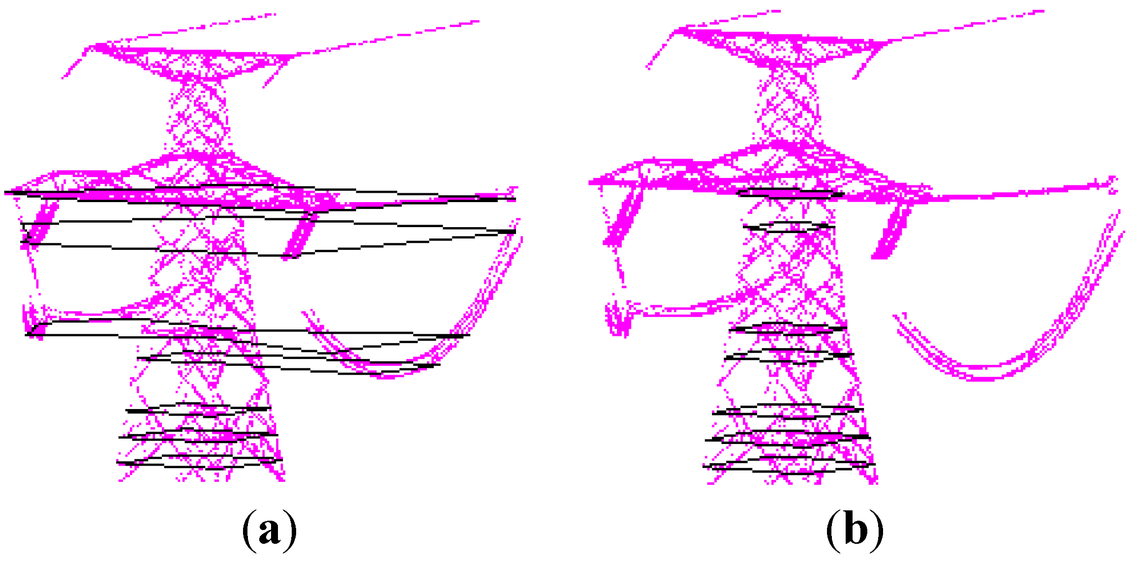
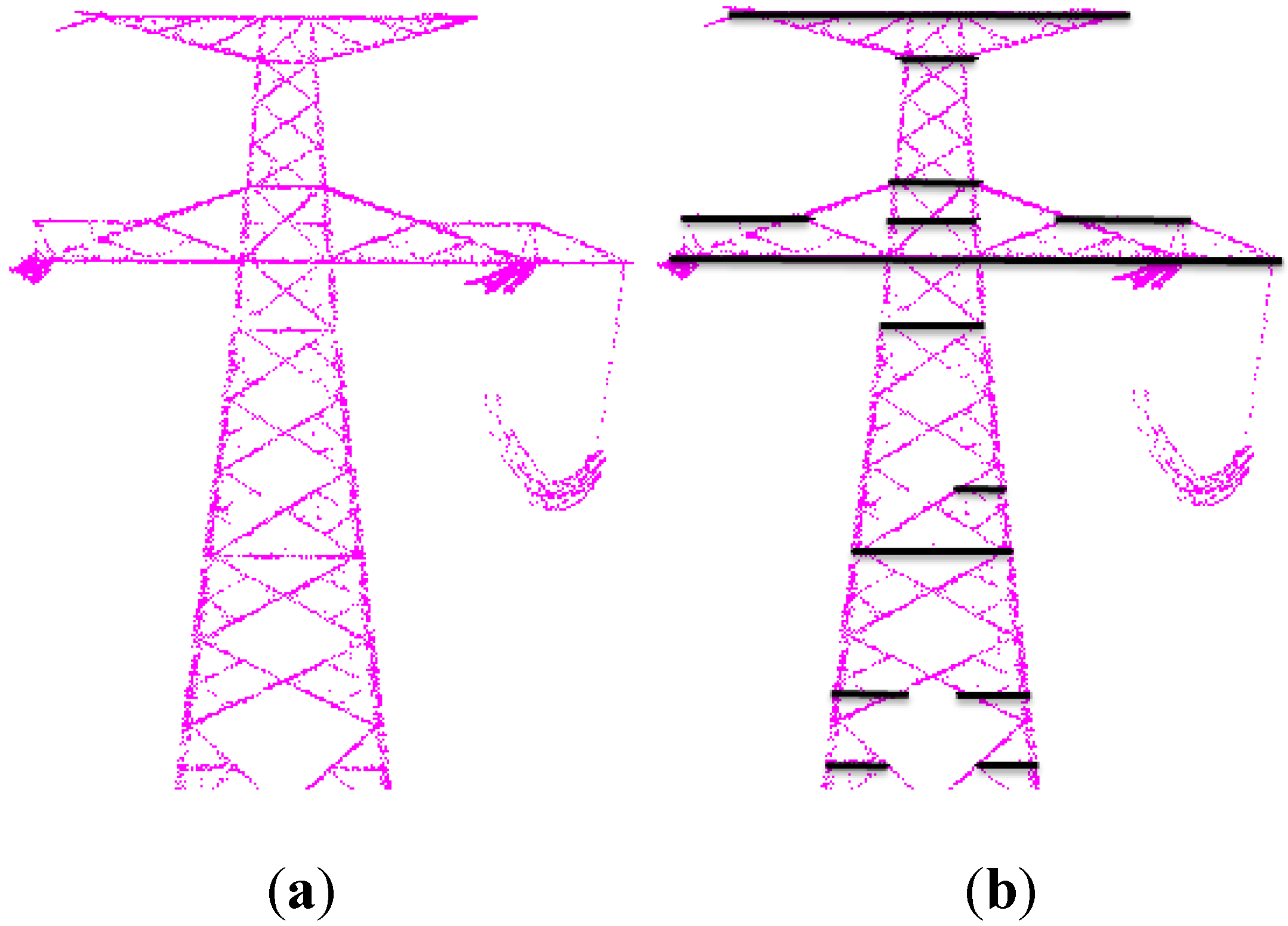
28] proposed a method base on Markov Random Field (MRF) to classify key features (power lines, pylons, and buildings) that comprising utility corridor scene using airborne LiDAR data and model power lines in 3D object space. Since the geometry model of power line is relatively simple, the first step, separating power line points from background point clouds correctly, is the most significant issue in the power line reconstruction.
Generally, most of the existing 3D modeling methods based on point clouds is designed for specific modeling object. Due to the different distribution characteristics of different modeling target point clouds, these methods are difficult to be applied directly on the automatic three-dimensional reconstruction of pylon.

1.2. Our Contribution

In this paper, we promote a solution that reconstructs the pylon model of high-voltage transmission for smart grid safety and 3D visualization application. We first define a general parametric pylon model based on some observations of the point clouds and existing vector models of several types of pylon. A practical segmentation method is used to detect the pylon points for further individual pylon modeling. We use a height histogram method that decomposes a pylon into three simple parts. The head of pylon is reconstructed through a pre-build library if the type is determined. Furthermore, the body of pylon is reconstructed by least square fitting with additional constrains.
In the rest of this paper, Section 2 defines the pylon parametric model and describes the modeling workflow. Section 3 discusses the pylon segmentation, orientation and position method, modeling of pylon head and body. Experiments and results are discussed in Section 4. Finally, Section 5 gives the conclusions of the proposed approach and future work.

2. Overview of Our Approach

Due to some intrinsic imperfections (e.g., uneven distribution, incompleteness and noise) in ALS point clouds, model-drive method is preferred for pylon reconstruction. As the pylon is a complicated truss construction (Figure 1), a variety of actual pylon structures as well as characteristics of point clouds data are reviewed to derive a practical parametric model. Then a model-driven method is applied to the three-dimensional reconstruction of the specific self-supporting pylon. First, the complex power pylon is segmented into several simple parts. Then each part is reconstructed with different strategies. At last, they are assembled according to position and direction information.
Figure 1. Pylon model and point cloud: (a) Pylon model, (b) pylon point cloud, and (c) noisy points.
Remotesensing 07 11501 g001

2.1. Pylon Parametric Model

Pylons in China can be divided into self-supporting pylon and guyed pylon according to their structure [29]. This paper mainly studies the most commonly applied self-support pylon with four legs (Figure 1), which has the following characteristics:
(1)
There are four legs in a pylon. Each of them is an inverted three-pyramids and their size may vary from terrain to terrain.
(2)
The pylon body is a simple quadrangular frustum pyramid.
(3)
The structure of pylon head is more complicated. There exist distinguishing features between different types of pylons, while structures of pylon heads with the same type are strictly consistent. So a pylon can be classified into a certain class according to its head type.
Based on these characteristics, a self-supporting pylon is described as an integrated model which is composed of: pylon legs, pylon body and pylon head determined by four remarkable structure heights: the foot height, the body height, the shoulder height and the head height. A local right hand reference frame attached to the pylon is built with its origin in the center of pylon top, x axis pointing to direction of pylon cross arm and z axis vertical (Figure 2a). Therefore its origin ( x 0 , y 0 , z 0 ) represents the pylon’s position and x axis indicates the pylon’s orientation ( φ ). The head is decided by its type   T c . The body can be depicted by intersecting four planes P i , and two stricter heights, H s and H b . The legs can be decided by four points P t i . So a pylon can be determined by a parameter Equation (1).
p y l o n = [ x 0 y 0 z 0 φ T c H s H b P i P t i ]
where i = 1 , 2 , 3 , 4 .
Corresponding to the actual structure, pylon point clouds have the following distribution characteristics:
(1)
Distribution of the head points is quite complicated due to the complexity of the head structure. There are power lines points distributed close to the head points. In addition, the point cloud of the head may be incomplete during data acquisition.
(2)
There are some power line points near the body and points of it may be incomplete due to occlusion and a low scan frequency of LiDAR.
(3)
Usually, noisy points, such as terrain points and plant points, among the pylon leg points exist.
(4)
The pylon structure can be clearly presented in the front and side view of the point cloud (Figure 2b).
Figure 2. Pylon parametric model. (a) 3D view, (b) Front view, (c) Side view, (d) Vertical view.
Remotesensing 07 11501 g002

2.2. Workflow for Pylon Modeling

Based on the characteristics of pylon structure and coresponding point cloud, the modeling procedure is presented. Pylons are detected and segmented from the corridor point cloud first, then an individual pylon is reconstructed. Noting that the point density and shape of pylon is distinct from that of power line, it can be detected by a practical segment process of the point clouds. When it comes to an individual pylon, for the complicated structure of its head, it is challenging to infer the topological relationship between the surfaces and lines using a data driven method. However, the structure of the pylon head with the same type is strictly consistent. Therefore, it can be modeled with a pre-build head model library if the head type is known, which can be determined by a classifier. The structure of pylon body is a regular quadrangular frustum pyramid. It is easy to infer the position and orientation and the model of the body by combining the four planar surfaces on its side. The scene of point clouds of pylon leg is quite complex due to the noisy points of terrain, plants, etc. Thus, an interactive modeling method may be preferred for it. This will not be discussed in this paper. The proposed modeling method consists of several steps, as follows (Figure 3).
(1)
Pylon detection: Pylons are detected from transmission corridor point clouds.
(2)
Pylon segmentation, positioning and orientation: A pylon is decomposed into head, body and legs by its structure height. After that, the position and orientation are derived from the body.
(3)
Modeling of pylon head: Pattern features of head are extracted from height histogram and front projection of the pylon head points, its type is decided by SVM (Support Vector Machine) classification method. The head is modeled once through matching with the head model library.
(4)
Modeling of pylon body: The pylon body is modeled by intersecting the adjacent body side planes that derived from a constrained plane fitting process.
(5)
Modeling of pylon legs: The rest of the pylon is modeled manually with the aid of previous modeling results.
In this paper, only Steps 1–4 are discussed in detail.
Figure 3. Workflow of pylon modeling.
Remotesensing 07 11501 g003

3. Methodology

3.1. Pylon Detection

The raw data we used in this paper is corridor point clouds in which terrain points have been filtered out in advance by software. It contains power line points, pylon points and a small quantity of noisy points such as terrain, plants and so on. It is necessary to separate the points of an individual pylon before modeling. Power line points appear as thin lines, while the pylon appears as blocks in the vertical projection (Figure 4). The heights of power line points in the same projection grid vary in a small range while those of pylons vary in a greater range. Based on these findings, a practical algorithm (Algorithm 1) is proposed to detect pylons through the density projection image and height variance image of corridor point clouds. These parameters involved in Algorithm 1 all have an explicit physical meaning, based on which the empirical values are set (Table 1).
Figure 4. Point cloud projection images: (a) point density projection image; and (b) point height variance image.
Remotesensing 07 11501 g004
Algorithm 1 Pylon detection
Input: corridor point clouds P c o r = { ( x i , y i , z i ) | i = 1 , 2 , n , n is the number of points;
Output: Individual pylon points   P p y l o n = { P j | j = 1 , 2 m } , m is the number of pylons.
1:
Generate the point density projection image I 1 (Figure 4a) and point height variance image I 2 (Figure 4b) of corridor point clouds with grid size g d . The pixel values of I 1 equal the counts of points in the corresponding grids. The pixel value of I 2 is height variance of points of each grid.
2:
Use a window with a disk kernel of size S to slide along the nonzero pixels on image I 1 . The response image I 3 is the total number of points within the slide window.
3:
Select the local maximum pixel with a suppression range r s as the candidate center of pylons.
4:
Count the number of high value (greater than t v ) pixels in image I 2 in the disk kernel of the each candidate centers and donate them as N . The centers whose N value is greater than t a are regard as the final pylon centers.
5:
Return: Points P j in the circle range with a radius r p of pylon centers.
Table 1. Physical meaning and empirical values of parameters in Algorithm 1.
ParametersPhysical MeaningEmpirical Value
g d The ground distance of one pixel0.5 m
r s The smallest distance between two nearby pylons20 m
t v The threshold to judge if a grid is a pylon grid or a power line grid since pylon grid have greater height variance.3 m
S The size of a pylon11 m
t a The ratio of high variance pixels count to the sum of disk kernel pixels0.2
r p The range of possible pylon points r p = 1.5 * s

3.2. Pylon Segmentation, Position and Orientation

A robust method for pylon decomposition should follow a noise filtering process and one of the decomposed parts, known as pylon body, will be used to derive the position and orientation.

3.2.1. Filtering

There usually exist several kinds of noisy points in the auto-detected pylon points (Figure 1) as we have mentioned in Section 2.1. Their distribution characteristics are summarized below:
(i)
Terrain and plants points often aggregate near the pylon legs.
(ii)
Power line points around the body are usually relatively far from the pylon horizontal center.
(iii)
Power line points close to the head are hard to separate. However, this has little effect on the pylon head modeling result due to the model driven method we take.
A progressive filtering strategy is applied in this paper: using the extracted information, exclude the noise step-by-step during the whole modeling process until the modeling process finishes. On the basis of case (i), we filter out points under a height threshold T h (where T h = H r + C , H r stands for the lowest elevation of pylon points, C is a constant which is decided by the pylon structure empirically). As for power line points in case (ii), they are removed according to the horizontal distance to the pylon center.

3.2.2. Decomposition

The horizontal component of a pylon distributed appears as high amount of points at a height interval (Figure 5). The plane of the horizontal component is called feature plane and its height is defined as feature height. When the histogram is counted against the height level, the local maximums probably correspond to feature heights (Figure 5c).
Figure 5. Segmentation based on feature heights histogram: (a) pylon model; (b) constrain length; (c) height histogram; and (d) point cloud and feature heights. Horizontal members are high lightened with magenta color in (a,b). Height histogram is shown in (c). Feature heights are marked with short lines.
Remotesensing 07 11501 g005
In the height histogram, not all local maximums correspond to pylon feature height, and the distribution of them are irregular (Figure 5c). What is more, the values of them vary with the density of point cloud. Therefore, it is hard to extract these heights by simple local extreme value analysis or threshold methods. The interval between neighboring feature height is greater than a certain threshold value (Figure 5b). A detailed extraction algorithm is presented as follow:
Algorithm 2 Feature heights extraction
Input: pylon point clouds P p y l o n = { P i | i = 1 , 2 n } , n is the count of points;
Output: pylon feature heights H f e a t u r e = { H j | j = 1 , 2 , , m } , m is the count of feature heights
1:
Generate the histogram of height of P i with a certain bin width H .
2:
Seek N t largest heights with the histogram values as candidate feature heights (Figure 6a)
3:
use a window with size of L c to move forward and backward to extract the local maximums (Figure 6b,c). Select the consistent local maximums in two processes as the initial feature heights H j i n i t (Figure 6d).
4:
Select points p = { p i | z i [   H j i n i t ε , H j i n i t + ε ] } , calculate the mean value of { z i } iteratively and eliminate gross errors and yield the refined feature heights   { H j } .
5:
Return: { H j } .
It is assumed that the feature height below tower top in a certain range with the most points correspond to the shoulder height, i.e., the height where the body and head join. The head and body can be separated by this height (Figure 5c). Since the shoulder height value equals the top height minus the height of head, it can be calculate and validated once the type of pylon head is determined.
Figure 6. Extracting local maximums from height histogram with constraint (Lc = 6): (a) points elevation histogram; (b) forward extracted local maximums; (c) backward extracted local maximums; and (d) final extracted local maximums.
Remotesensing 07 11501 g006

3.2.3. Extraction of Orientation and Position

The feature planes on pylon body are a group of vertically distributed rectangles with an approximately consistent horizontal center (Figure 7a). These rectangles shrink from the bottom to the top. That helps to obtain a robust estimation of orientation and position of the pylon.
Figure 7. Contours analysis: (a) feature plane; (b) circumcircles; (c) α-shapes contour; and (d) simplified contour.
Remotesensing 07 11501 g007
For points on each feature plane, the α-shapes algorithm [30] is applied to generate the convex contour of each, then the plane center coincides with the center of its circumcircle. The horizontal position of pylon is derived from the average center of each circumcircle (Figure 7b).
Short line segments in the primitive contours, which appear to zigzag, are merged into long ones (Figure 7c) to infer the pylon orientation. This is achieved by the pipe algorithm [31]. Direction of the longest line segment in each merged contour is treated as the pylon orientation (Figure 7d). Again, the averaging operation is conducted to obtain the orientation of the whole pylon. During estimation of the position and orientation, gross errors derived from each contour are removed using RANSAC. Finally, the average values are regarded as accurate position and orientation.
Suspension power line points would disturb the contour generation if not eliminated (Figure 8a). Noticing that rectangles at lower heights are larger than those at higher heights, we first extract contours from the bottom. The smallest extracted contour is used to limit the scope of the next feature plane to eliminate power line points before α-shapes algorithm process (Figure 8b).
Figure 8. Power line noise’s influence on α-Shapes results: (a) before eliminating noise; and (b) after eliminating noise.
Remotesensing 07 11501 g008

3.3. Pylon Head Modeling Method

Due to the consistence of pylon heads with the same type, the key issue in reconstructing this component is determination of its type, position and orientation.

3.3.1. Features of Head

In order to decide the type of a given head, pattern features that describe the type are extracted first. Then the type can be judged automatically by classification technic. Two kinds of features are designed for the pylon head, which are based on the point height histogram and front projection image.
Features based on point height histogram: There are some interesting characteristics in the point height histogram of a pylon head. Firstly, pylon heads of the same pe present similar feature heights in the histogram (Figure 9). Another stable characteristic is the maximum value, which corresponds to the horizontal component with the most steel of the head. On the basis of these, three robust features can be extracted by calculating the differences between some semantic feature heights and the mentioned stable height. Thus, a feature vector F 1 = [ H 1 H s , H 2 H s , H 3 H s ] is generated. Table 2 gives the semantics of these feature heights in detail.
Table 2. Feature heights derived from the histogram.
Feature ElevationSemantics
H s height of the most points
H 1 first feature height above H s
H 2 feature height of the most points above H s
H 3 feature height closest to pylon top
Figure 9. Point cloud height histograms of the same type pylons.
Remotesensing 07 11501 g009
Features based on front projection image: Pylon is a symmetrical truss artificial construction. When rotating to the front or side view (Figure 2b), its dimension is reduced from 3D to 2D and the feature extraction can be simplified. The front view image contains the most information including the vertical and horizontal structure variable of a pylon. Thus, it can be used to extract features of the head. Before further processing, the point clouds are rotated by the extracted pylon orientation ϕ, making the pylon cross arm pointing to the y-axis of world coordinate system.
After that, points on a feature height are project into a line image. Adjacent lines on this image are merged and short lines are removed on each feature height. The feature lengths and difference of their corresponding heights are taken as features (Figure 10). Two kinds of feature lengths of each feature height are defined: the one is span length, i.e., the span of all horizontal members; the other is physical length, i.e., the actual length of all horizontal members. The detail algorithm is shown below:
Algorithm 3 Feature length extraction based on front projection
Input: pylon point clouds P i = { x i , y i , z i } , extracted feature height H f e a t u r e = { H j } ;
Output: pylon head features F 2
1:
project points at a certain feature height  p = { p i | z i [   H j i n i t ε , H j i n i t + ε ] } ), to a line array according to the x coordinate value. If there are no points in a grid, the value of the grid is 0 , otherwise it is 1 (Figure 11).
2:
Merge adjacent non-empty grids if the gaps between them are less than a certain threshold t g a p (Figure 11b). Right after that, eliminate continuous non-empty grid sequences with length less than a certain threshold t l e n g t h (Figure 11c).
3:
Calculate the span length and physical length on each feature height. The span length L s equals to the distance of the leftmost non-empty grid to the rightmost one. The physical length L p equals to the summed length of all non-empty grids at one feature height, i.e., L p = L p i (Figure 11c).
4:
Find the largest and second largest span length L s 1 , L s 2 and heights H L s 1 , H L s 2 corresponding to them, the largest and second largest physical length and corresponding heights. Take F 2 = [   L s 1 ,   L s 2 ,   L p 1 ,   L p 2 , H s , H p ] as the features of pylon head, where H s = |   L s 1   L s 2 | , H p = |   L p 1   L p 2 |
5:
Return: F 2
Figure 10. Result of feature length extraction: (a) front view; and (b) result of feature lengths.
Remotesensing 07 11501 g010
Figure 11. Extract feature length based on front projection. (a) Point cloud projection; (b) line connection; and (c) eliminate short lines.
Remotesensing 07 11501 g011

3.3.2. Classify Pylon Head with SVM

By combining the previously derived features together, the unique descriptor for a pylon head is obtained. Taking the consistency of head type into account, the classification method can achieve an efficient 3-dimensional reconstruction. Once the type is determined, the shape model is selected from a prior library and fitted to the point cloud. Support vector machines, proposed by Cortes and Vapnik [32], initially aim to make a small training set classifier that can be applied in large-scale data classification, which means strong generalization ability. That property accords with the requirement for pylon reconstruction since the number of samples is relatively limited. A model library of some typical heads and a classifier trained with some head samples is constructed first. Once the type is determined for a new head, the previously derived orientation and horizontal position and its own height is used to fit the final shape for the particular point cloud.
In this paper, the LibSVM package of SVM algorithm [33] is used to classify the extracted pylon. The kernel function of the classifier is radial basis function (RBF). In the RBFSVM model, index parameter λ and the penalty factor C in objective function is decided through the grid parameter search during the training stage, it selects the best cross-validation accuracy corresponding the λ and C parameters in order to make the classifier to obtain the best generalization ability, i.e., classifier with less training data but better generalization ability. Therefore workload of classifier training in the pylon head modeling process is reduced.

3.4. Reconstruction of Pylon Body

Pylon body is a regular quadrangular frustum pyramid (Figure 12a). For a robust body framework model, a fitting method is employed for the modeling process. At first, the pylon body is segmented into four side planes. Next, it is fitted to a whole quadrangular frustum pyramid, i.e., fit the plane considering the symmetrical and perpendicular relationship of the body sides. Finally, the body framework is generated by intersecting the adjacent side planes.
Figure 12. Pylon body fitting: (a) feature planes; (b) segmentation; (c) vertical view of segmentation; and (d) body framework.
Remotesensing 07 11501 g012

3.4.1. Body Side Plane Segmentation

When the point cloud is sufficiently dense, we assume that points in the body feature plane contours extracted by α-shapes algorithm can represent the body. In order to identify points belong to which side, we need to identify its corresponding contour edge belong to which side. This is achieved by classifying the edges of α-shapes contour into four groups according to their orientation. If the orientation of a contour edge is close enough to one of the four orientations of body sides, the two endpoints of the edge are classified to the corresponding side (Figure 12b,c) otherwise they will be removed.

3.4.2. Pylon Body Fitting

The body is fitted to a quadrangular frustum pyramid whose center axis is vertical (Figure 12d). This problem can be modeled as a least squares fitting with additional parameters. That means the four sides are fitted to planes considering that the XOY projection of adjacent side normal vectors are perpendicular and the sides opposite to each other are symmetrical with the center axis. These constraints are added into the adjustment model. That will overcome the adverse impact caused by sparseness or incompleteness of points on body sides.
The general function model of the least squares fitting with additional parameters can be express as Equation (2), where L ˜ refers to the observation values, and X ˜ refers to the additional parameters.
F ( L ˜ , X ˜ ) = 0
There are two types of error equations for this fitting problem: the ones are equations where the observations meet, the others are equations where the plane parameter meet. Observations satisfy the conditional equation, i.e., plane condition equations. Each point can form one equation. The 12 coefficients of the four planes are additional parameters. The number of additional parameter conditions is five in total. Total number of equations is N + 5, where N is the points of pylon body side planes. The unknown value to solve is plane parameters corrections.
The planar conditional equations that points on the four body side satisfy, as Equation (3):
A i x i j + B i x i j + C i z i j + 1 = 0
The constrain equations that plane coefficients satisfy:
Perpendicular constrains of adjacent side, as Equation (4):
{ A 1 × A 2 + B 1 × B 2 = 0 A 2 × A 3 + B 2 × B 3 = 0 A 3 × A 4 + B 3 × B 4 = 0
Symmetrical constrains of opposite side, as Equation (5):
{ C 1 / A 1 2 + B 1 2 C 3 / A 3 2 + B 3 2 = 0 C 2 / A 2 2 + B 2 2 C 4 / A 4 2 + B 4 2 = 0
Linearization and iterative solution are needed to solve these nonlinear error equations. The initial values of side planes parameters are set by plane fitting. Since noise points on the contours may disturb the final result seriously, RANSAC method is used in plane fitting to eliminate gross errors before global adjustment. Finally, fit four planes intersection lines to obtain the framework of the pylon (Figure 12d).

4. Experiments and Result

4.1. Dataset

For verifying the effectiveness of the proposed method, several experiments are conducted on the airborne LiDAR data of transmission corridors from China Southern Power Grid. The raw data is collected by a Harris 56 laser scanner attached to a helicopter. The flight height is about 300~400 m. The density of points is about 40/m2 on average. Six transmission lines point cloud data are used for pylon detection and six types of 157 pylon samples whose types have been labeled manually are used for individual pylon modeling.

4.2. Result and Discussion

4.2.1. Pylon Detection

In this experiment, pylons are automatically detected and extracted from six transmission lines point cloud data. The correctness and completeness of the result (Table 3) are evaluated according to the Equation (6), where T P   is the number of correctly extracted pylon, F P   refers to the number of pylon mistakenly extracted, and F N   refers to the number of missing power towers. The missing extracted pylons are mainly guyed style (Figure 13b), not the four-leg style that is studied in this paper, because they were filtered out by a high value area threshold t a . The experimental results show that the proposed algorithm is effective at separating a single pylon from massive point clouds.
Figure 13. Missing detected guyed pylons: (a) point cloud; and (b) vertical view.
Remotesensing 07 11501 g013
{ C o m p l e t e n e s s = T P / ( T P + F N ) C o r r e c t n e s s = T P / ( T P + F P )
Table 3. Pylon detection result. Note: N is the umber of points.
Dataset N T P F P F N CorrectnessCompleteness
11,321,5414800100%100%
2665,583380490%100%
3642,1541300100%100%
41,219,018410295%100%
51,884,0656600100%100%
61,326,5395420100%96%
Sum7,058,9002602698%99%

4.2.2. Structure Heights of Different Types of Pylon

The structure height of pylon is a significant parameter of pylon model. The difference of pylon top height and shoulder height of different types of pylons are measured, and the standard deviations are calculated (Table 4). The result indicated that the differences are almost identical if the pylon types are the same. Hence the differences of structure height can be features that characterize pylon head.
Table 4. The top height and shoulder height difference of pylons with different types.
IndexType 1Type 2Type 3Type 4Type 5Type 6
114.07517.01018.51813.78112.9848.627
214.09717.00318.54013.79812.9908.612
314.09117.00218.54213.76812.9808.624
414.08417.01218.53213.74712.9958.599
514.09017.01218.54213.78612.9768.595
614.08417.00018.52713.75713.0098.612
714.09716.99818.51213.74912.9958.601
814.08717.00318.54613.74012.9898.594
Standard deviation0.0070.0060.0120.0210.0100.013

4.2.3. Precision of Pylon Horizontal Position and Orientation

In this experimentation, the proposed modeling method is applied on the 157 pylon samples. Table 5 shows the precision of automatically extracted horizontal center position and orientation from each pylon on average as well as their standard deviation. δ x , δ y stand for the average precision of x position and y position, respectively; and δ d represents the average precision of orientation. They are defined by Equation (7):
{ δ x = δ x i / n δ y = δ y i / n δ d = δ d i / n
where n is the total number of pylons, i = 1 , 2 , 3 , 4 , δ x i , δ y i , δ φ i stand for the position and orientation precision of pylon i, which are standard deviations of ( x i j , y i j ) and φ i j of pylon body feature contours after removing the gross errors; j is the number of body feature contours those without gross errors.
The result indicated that the precision of pylon horizontal position reached 0.03 m and that of the pylon orientation reached 0.99°. They are both accurate enough for pylon visualization application.
Table 5. Precision of pylon horizontal position and orientation. Note: N is the point number of pylon, H is the height of pylon.
Pylon Index N N / H (m) δ x (m) δ y (m) δ d (°)
16349155.00.0460.0400.418
213,050291.70.0110.0230.287
39873224.20.0430.0161.317
411,132268.30.0210.0080.208
55291118.40.0260.0442.280
611,859260.50.0200.0190.853
7362197.90.0260.0270.709
8478692.60.0490.0411.397
9216347.20.0470.0490.772
1054,1831191.60.0110.0150.599
118053189.60.0300.0302.118
1216,003393.00.0220.0150.587
136739157.00.0420.0290.427
14265651.10.0470.0491.608
15382377.00.0450.0310.910
1613,298315.00.0130.0130.309
1727,082594.00.0160.0190.680
1854,1831191.60.0110.0150.599
Mean14119317.50.0290.0270.893

4.2.4. Accuracy of SVM Classification

In this experiment, 157 pylon samples are grouped with five kinds of proportions randomly (1:1, 1:3, 1:5, 1:7, 1:9) for training and testing. Classifications based on two kinds of features combination are tested in this experiment. The three features combination is extracted based on the point height histogram and the six features combination is extracted based on the front projection image. The SVM with a RBF as basic function implemented by LibSVM is utilized for the training and testing. The test accuracy values based on different feature combinations are presented in Table 6.
Table 6. Classification accuracy. Note: Ns: number of all samples Ntr: number of train samples, Nte: number of test samples, Accuracy1: accuracy based on three features; Accuracy2: accuracy based on six features.
Ntr;NteNsNtrNteAccuracy 1 (%)Accuracy 2 (%)
1:1157787997.4798.73
1:31573911898.3199.15
1:51572613195.4298.47
1:71571913893.4895.65
1:91571514286.6295.77
The result of experiment suggests:
(a)
The classification accuracy of the test sample decreases as the ratio of training samples to test samples decreases. Dirty samples may have greater impact on the training results in the case of too few training samples, while too many training samples will make it inefficient. Therefore, an appropriate number of power tower samples data set for training is significant to promote the generalization ability and outreach capacity of classifier in the modeling process.
(b)
Comparing the classification accuracy of different features combinations, it is obvious that feature extraction method based on front projection image performs better, because this method extracts not only elevation features but also length features. What is more, the elevations are determined by the length features so that it can avoid the effect caused by noisy and result in robust features.
In conclusion, when taking proper feature extraction method and quantity of training samples, the proposed method can classify the head with accuracy higher than 95%.

4.2.5. Result of Pylon Body Fitting Accuracy

Results of 157 pylon body fitting accuracy are evaluated by the average distance of points to the corresponding side plane. Table 7 gives the result of six randomly selected types of 18 pylons. It demonstrates that the average distance of points to the side planes is about 0.05 m. Bad fitting results are usually caused by the sparseness, incompleteness of point cloud, so it is necessary to improve the density of raw data for more accuracy modeling result.
This paper has modeled the heads and bodies of 157 pylons with known types automatically using the proposed method. To visually check the result of the model, the pylon points and model are registered. Figure 14 shows the result of six different typical types of pylon and it can be seen that the models fit the points quite well, and this model can be applied in the digital power gird for visualization and some simple digital management.
Figure 14. Samples of six types of pylon modeling result.
Remotesensing 07 11501 g014
Table 7. Precision of body side planes fitting.
Pylon TypeNp1Residuals1Np2Residuals2Np3Residuals3Np4Residuals4
1160.034220.041190.036180.034
1400.044390.041270.075360.042
1210.043340.048390.039230.040
2130.084140.068310.056130.054
2190.05680.030170.037220.034
2110.09640.067290.038200.029
3290.044200.028360.033250.026
3340.063260.041220.086240.064
3710.167530.1271000.056480.034
4430.054310.040270.041220.047
4630.047300.024330.042270.034
4540.046270.031320.036160.044
5330.027160.061260.034330.027
5290.027210.045290.031280.025
5220.027240.029340.029200.043
6580.048350.053450.152300.070
6260.052380.042480.051310.057
6580.046630.051510.056420.047
Mean35.60.05628.10.04835.80.05126.60.042

5. Conclusions

In this paper, a parametric pylon model of high-voltage transmission is first constructed. A model driven 3D pylon reconstruction method is proposed based on this model. Pylons are detected and segmented from the transmission corridor point clouds by a practical segment process before modeling. For single pylon modeling, a complex pylon is first segmented into several simple parts. Then each part is reconstructed with different strategies and, finally, assembled according to position and orientation in consistent reference frame.
Noting that the point density and shape of pylon is distinct from that of power line, horizontal scope can be detected by a practical segment process of the point clouds, the completeness and correctness of the detection result are both higher than 90%. Local maximums in pylon point clouds height histogram can well reflect the structure of pylon. Segmentation of pylon points and extraction of the feature planes are achieved using the height histogram local maximums. Pylon position and orientation are derived by contour analyzing of the feature planes. The dimension of raw 3D data are reduced to 2 dimensions and 1 dimension though height histogram and front projection, which helps to mitigate the adverse impact of sparseness, incompleteness and noisy of raw data. This makes the process easier and more robust features with semantics. In order to evade the complexity of the head, the reconstruction method based on SVM classification is utilized. This method can determine the pylon type with accuracy higher than 95%. The body is reconstructed by least square fitting with additional constrains. The edges of body are precisely reconstructed by intersecting the side planes. Experiments on data sets from the South China Grid suggest that the proposed method can reconstruct the pylon get the head and body model automatically.
However, there are also several limitations in this method. Due to the conceptual pylon model, it is only applicable for pylons that fit the parametric model (i.e., pylons with four legs) of high-voltage transmission. Another limitation is the need for pre-build head model library, which is also the one limitation in most model driven methods. Additionally, the body reconstruction result would be susceptible to extreme sparseness of points on pylon body sides.
For higher accuracy applications, such as pylon force analysis, deformation monitoring and so on, it demands finer and more accurate pylon model. In addition, for pylon modeling of regional networks, the LiDAR data quality and complex pylon model library are the new challenge for the proposed approach. With the development of Airborne Lidar technique, high precision and density point clouds are available. Therefore, study of fine pylon modeling with high-density point clouds based on LiDAR techniques will be the future work.

Acknowledgments

The authors would like to express their gratitude to the editors and the reviewers for their constructive and helpful comments for substantial improvement of this paper, and to Doctor Peng Jianwei and Doctor Zou Qing in Wuhan University for polishing the language of this paper. This research is supported by National Natural Science Foundation of China (Grand No: 41271452), National Natural Science Foundation of China(Grand No:2012CB725300), Shenzhen Key Laboratory Construction Project (Grand No: ZDSY20121019111146499),Shenzhen Scientific Research and Development Funding Program (No. ZDSY20121019111146499) and Shenzhen Dedicated Funding of Strategic Emerging Industry Development Program (No. JCYJ20121019111128765).

Author Contributions

Qingquan Li and Qingwu Hu conceived the study and designed the experiments. Zhipeng Chen wrote the main program and most of the paper. Qingwu Hu published this paper.

Conflicts of Interest

The authors declare no conflict of interest.

References

  1. Xu, Z.; Yang, F.; Huang, Y.; Wang, Z.; Liu, Y. Lidar applications in the electrical power industry. Int. Arch. Photogramm. Remote Sens. Spat. Inf. Sci. 2008, XXXVII, 137–140. [Google Scholar]
  2. You, A.; Han, X.; Wang, X.; Tang, D. Applications of Lidar in Patrolling Electric-Power Lines. In Proceedings of the 2013 International Conference on Technological Advances in Electrical, Electronics and Computer Engineering (TAEECE), Konya, Turkey, 9–11 May 2013.
  3. Ussyshkin, R.V.; Theriault, L.; Sitar, M.; Kou, T. Advantages of airborne Lidar technology in power line asset management. In Proceedings of the 2011 International Workshop on Multi-Platform/Multi-Sensor Remote Sensing and Mapping (M2RSM), Xiamen, China, 10–12 January 2011.
  4. Maas, H.-G.; Vosselman, G. Two algorithms for extracting building models from raw laser altimetry data. ISPRS J. Photogramm. Remote Sens. 1999, 54, 153–163. [Google Scholar] [CrossRef]
  5. Tarsha-Kurdi, F.; Landes, T.; Grussenmeyer, P.; Koehl, M. Model-Driven and Data-Driven Approaches Using Lidar Data: Analysis and Comparison. Available online: https://halshs.archives-ouvertes.fr/halshs-00264846/document (accessed on 11 May 2015).
  6. Dorninger, P.; Pfeifer, N. A comprehensive automated 3d approach for building extraction, reconstruction, and regularization from airborne laser scanning point clouds. Sensors 2008, 8, 7323–7343. [Google Scholar] [CrossRef]
  7. Kada, M.; McKinley, L. 3d building reconstruction from Lidar based on a cell decomposition approach. Int. Arch. Photogramm. Remote Sens. Spat. Inf. Sci. 2009, XXXVIII, 47–52. [Google Scholar]
  8. Huang, H.; Brenner, C.; Sester, M. 3d Building Roof Reconstruction from Point Clouds via Generative Models; ACM: New York, NY, USA, 2011. [Google Scholar]
  9. Henn, A.; Gröger, G.; Stroh, V.; Plümer, L. Model driven reconstruction of roofs from sparse Lidar point clouds. ISPRS J. Photogramm. Remote Sens. 2013, 76, 17–29. [Google Scholar] [CrossRef]
  10. Fischler, M.A.; Bolles, R.C. Random sample consensus: A paradigm for model fitting with applications to image analysis and automated cartography. Commun. ACM 1981, 24, 381–395. [Google Scholar] [CrossRef]
  11. Lafarge, F.; Mallet, C. Building Large Urban Environments from Unstructured Point Data. In Proceedings of the 2011 IEEE International Conference on Computer Vision (ICCV), Barcelona, Spain, 6–13 November 2011.
  12. Overby, J.; Bodum, L.; Kjems, E.; Iisoe, P.M. Automatic 3d building reconstruction from airborne laser scanning and cadastral data using hough transform. Int. Arch. Photogramm. Remote Sens. 2004, 35, 296–301. [Google Scholar]
  13. Tarsha-Kurdi, F.; Landes, T.; Grussenmeyer, P. Hough-Transform and Extended Ransac Algorithms for Automatic Detection of 3d Building Roof Planes from Lidar Data. In Proceedings of ISPRS Workshop on Laser Scanning 2007 and SilviLaser 2007, Espoo, Finland, 12–14 September 2007.
  14. Tarsha-Kurdi, F.; Landes, T.; Grussenmeyer, P. Extended RANSAC algorithm for automatic detection of building roof planes from Lidar data. Photogramm. J. Finl. 2008, 21, 97–109. [Google Scholar]
  15. Verma, V.; Kumar, R.; Hsu, S. 3d Building Detection and Modeling from Aerial Lidar Data. In Proceedings of the 2006 IEEE Computer Society Conference on 2006 Computer Vision and Pattern Recognition, New York, NY, USA, 17–22 June 2006.
  16. Zhou, Q.-Y.; Neumann, U. A Streaming Framework for Seamless Building Reconstruction from Large-Scale Aerial Lidar Data. In Proceedings of the IEEE Conference on 2009 Computer Vision and Pattern Recognition, CVPR 2009, Miami, FL, USA, 20–25 June 2009.
  17. Elberink, S.O. Target graph matching for building reconstruction. Proc. Laserscanning 2009, 9, 49–54. [Google Scholar]
  18. Sampath, A.; Shan, J. Segmentation and reconstruction of polyhedral building roofs from aerial Lidar point clouds. IEEE Trans. Geosci. Remote Sens. 2010, 48, 1554–1567. [Google Scholar] [CrossRef]
  19. Lafarge, F.; Mallet, C. Creating large-scale city models from 3d-point clouds: A robust approach with hybrid representation. Int. J. Comput. Vis. 2012, 99, 69–85. [Google Scholar] [CrossRef]
  20. Lafarge, F.; Alliez, P. Surface reconstruction through point set structuring. Comput. Graph. Forum. 2013, 32, 225–234. [Google Scholar] [CrossRef]
  21. Kada, M.; Wichmann, A. Feature-driven 3d building modeling using planar halfspaces. ISPRS Ann. Photogramm. Remote Sens. 2013, II-3/W3, 37–42. [Google Scholar] [CrossRef]
  22. Wichmann, A.; Kada, M. 3D building adjustment using planar half-space regularities. ISPRS Ann. Photogramm. Remote Sens. Spat. Inf. Sci. 2014, 1, 189–196. [Google Scholar] [CrossRef]
  23. Xiong, B.; Jancosek, M.; Elberink, S.O.; Vosselman, G. Flexible building primitives for 3d building modeling. ISPRS J. Photogramm. Remote Sens. 2015, 101, 275–290. [Google Scholar] [CrossRef]
  24. Xiong, B.; Elberink, S.O.; Vosselman, G. A graph edit dictionary for correcting errors in roof topology graphs reconstructed from point clouds. ISPRS J. Photogramm. Remote Sens. 2014, 93, 227–242. [Google Scholar] [CrossRef]
  25. McLaughlin, R.A. Extracting transmission lines from airborne Lidar data. IEEE Geosci. Remote Sens. Lett. 2006, 3, 222–226. [Google Scholar] [CrossRef]
  26. Jwa, Y.; Sohn, G.; Kim, H.B. Automatic 3d powerline reconstruction using airborne Lidar data. Int. Arch. Photogramm. Remote Sens. 2009, 38, 105–110. [Google Scholar]
  27. Kim, H.B.; Sohn, G. 3D classification of power-line scene from airborne laser scanning data using random forests. Int. Arch. Photogramm. Remote Sens. 2010, 38, 126–132. [Google Scholar]
  28. Sohn, G.; Jwa, Y.; Kim, H.B. Automatic powerline scene classification and reconstruction using airborne Lidar data. ISPRS Ann. Photogramm. Remote Sens. Spat. Inf. Sci. 2012, 1–3, 167–172. [Google Scholar] [CrossRef]
  29. Huiming, S. Research and Application of Optimal Design Method of High Voltage Transmission Tower Structure; Guangzhou University: Guangzhou, China, 2011. [Google Scholar]
  30. Edelsbrunner, H.; Mücke, E.P. Three-dimensional alpha shapes. ACM Trans. Graphics 1994, 13, 43–72. [Google Scholar] [CrossRef]
  31. Shen, W.; Li, J.; Chen, Y.-H.; Deng, L.; Peng, G.-X. Algorithms study of building boundary extraction and normalization based on Lidar data. J. Remote Sens. 2008, 5, 692–698. [Google Scholar]
  32. Cortes, C.; Vapnik, V. Support-vector networks. Mach. Learn. 1995, 20, 273–297. [Google Scholar] [CrossRef]
  33. Chang, C.-C.; Lin, C.-J. LIBSVM: A library for support vector machines. ACM Trans. Intell. Syst. Technol. 2011. [Google Scholar] [CrossRef]

