Removal of Thin Clouds in Landsat-8 OLI Data with Independent Component Analysis

Abstract

An approach to remove clouds in Landsat-8 operational land imager (OLI) data was developed with independent component analysis (ICA). Within cloud-covered areas, histograms were derived to quantify changes of the reflectance values before and after the use of the algorithm. Referred to a cloud-free image, changes of histogram curves validated the algorithm. Scatterplots were generated and linear regression performed for the reflectance values of each band before and after the algorithm, and compared to those of the reference image. Band-by-band, results in cloud removal were acceptable. The algorithm had little effect on pixels in cloud-free areas after the analyses of histograms, scatterplots, and linear regression equations. Finally, the algorithm was applied to various land use and land cover types and cloud conditions, and to a full Landsat-8 scene yielding satisfactory results efficiently.

1. Introduction

Landsat-8 was launched into space in February of 2013. The success in data collection has operationally ensured the data continuity from Landsats-4, -5 and -7 to current Landsat-8 in acquisition geometry, multispectral characteristics, and ground coverage as well as radiometric and geometric calibration. Together, Landsat data allow us to study global agriculture, forestry, geology, land use and land cover (LULC) change, mapping, and regional planning over a time span nearly 40 years [1]. In addition, a coastal/aerosol band (Band 1, 433–453 nm of wavelength), a cirrus band (Band 9, 1360–1390 nm of wavelength), and a quality assessment (QA) band are added to Landsat-8 so that the needs of scientific studies and routine operations can be better met. The inclusion of Band 9 and QA band also stimulates the study of the cloud removal using one single Landsat-8 image (e.g., [2,3]).

Clouds in the atmosphere are located between spaceborne optical sensors and targets on the Earth’s surface. As solar radiation travels through clouds, the ice crystals and water vapor in the clouds cause scattering and absorption and can influence the transmission of the radiation. Thus, the satellite remote sensing data in the optical region are affected. Without the correction of the cloud effect, results derived from the data can be erroneous (e.g., [3,4]). Therefore, the removal of cloud effect is necessary.

Numerous methods such as image filtering, replacement, and transformation have been developed to remove clouds. The filtering approach operates in the frequency domain. As clouds are usually made of low frequency components, a high-pass filter such as the homomorphism filter [5,6] is capable of removing the clouds after filtering the data. However, the cut-off frequency to separate the high and low frequency components is empirically determined. The filter could affect the spectral characteristics of pixels in cloud-free areas as well. The image replacement approach uses either multi-temporal images [7,8,9] or a single image [3,10]. As long as there is a cloud-free image available on another acquisition date, the multi-temporal image replacement is feasible. Unfortunately, the success of the replacement is adversely affected by the temporal variation of the ground targets between two acquisition dates.

Coupled with Band 9 and QA band, Shen et al. (2015) [3] developed an image replacement approach using one single image to remove clouds for Bands 1–5 of Landsat-8. However, there are four main concerns with that method [3]. First, QA band data are used, and thermal infrared (TIR) data are needed to create the QA band. A majority of current operational optical sensors in space do not have one single TIR band [11]. Second, the replacement relies on the ability of Band 6 (1560–1660 nm of wavelength) and Band 7 (2100–2300 nm of wavelength) to penetrate the clouds. If there is doubt in the penetration, the replacement can be questionable. Third, if the cloud-covered area is over a water surface or the cloud-free area is water, the replacement can be erroneous because water absorbs almost all the solar radiation in Bands 6 and 7. Finally, the possible existence of cloud effects on Bands 6 and 7 are not considered.

As long as there is an image, image transformation can always be performed. The noticeable transformation approaches related to cloud/haze include the haze optimized transformation (HOT) [12], and extension of the original Tasseled Cap transformation [13]. The HOT approach is based on a defined “clear line” (CL) in a two-dimensional scatterplot between two spectral bands using reflectance values from pixels of cloud-free areas. The distance of every pixel to the CL is measured as the HOT response, which represents haziness [12] or cloud. After the quantification of the offset values of pixels grouped within a certain range of HOT levels relative to the histogram of the clear regions, the reflectance from the cloud of a pixel is removed by subtracting the individual offset value. Unfortunately, when the HOT is applied to land cover types of very high or low reflectance values in visible bands, the HOT is insensitive to the types. Thus, the cloud removal is ineffective [14]. Of the Tasseled Cap transformation, the fourth component is identified as haziness that is regarded as the cloud component in Landsat TM/ETM+ data [15,16]. The cloud component for Landsat-8 data is yet to be developed, although the Tasseled Cap transformation using Landsat-8 data has been studied [17,18].

The cloud detection using the independent component analysis (ICA) has been reported [19,20,21], but cloud removal using the ICA has not been studied. Therefore, we investigate an image transformation approach using the ICA to remove clouds in visible and infrared bands (Bands 1–7) of Landsat-8 operational land imager (OLI) data. Once the cloud reflectance of each pixel in each band can be estimated, the correction of clouds is simply a subtraction. The effectiveness of the ICA method is also assessed qualitatively and quantitatively.

2. Methodology

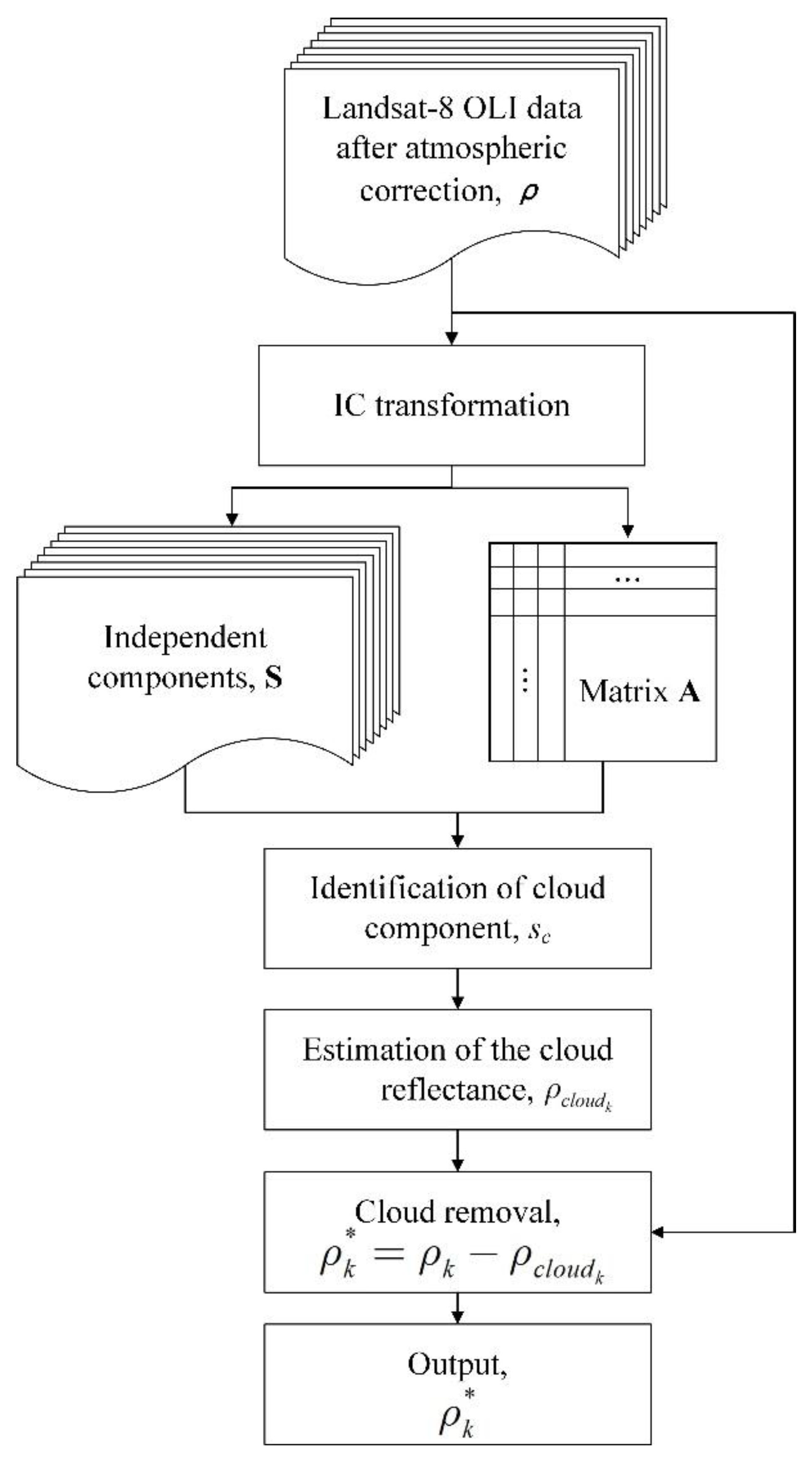
2.1. An Algorithm to Remove Clouds Using ICA

ICA is a technique of blind source separation that partitions independent sources from their liner observations [22,23]. The ICA is widely used in classification, change detection, and feature extraction [24]. An approach to remove clouds in Bands 1–7 of Landsat-8 data is explored using the ICA coupled with Band 9. The reason to add Band 9 in the algorithm is because each independent component (IC) is the linear mixtures of Landsat-8 Bands 1–7 and 9. Although the physical meaning of each IC is usually unclear, the absolute weight value from Band 9 related to each IC is used to delineate cloud component in the ICs. Therefore, we are able to remove the clouds in Bands 1–7.

Let ρ be the linear mixtures that are observed from n ICs or

$$\mathbf{\rho }\mathbf{=}\mathbf{A}\mathbf{S}$$

(1)

where S with elements s₁, …, and s_n is the column vector of ICs. Square matrix A with elements a_ij (i, j ∈ [1, …, n]) represents the linear transformation. ρ is the linearly mixed column vector and consists of elements ρ₁, …, and ρ_n. In this study, ρ₁, …, and ρ_n represent reflectance data of Bands 1–7 and 9. Thus, n = 8. Equation (1) can be also expressed in scalar form as

$${\mathrm{\rho }}_i={\displaystyle \sum _{j=1}^n{a}_{ij}{s}_j}.$$

(2)

Equation (1) or (2) is the ICA describing how mixtures are generated. A and S are unknown and can be estimated from ρ using the ICA as long as two assumptions that s_j is statistically independent to each other and s_j is not normally distributed are met.

The relationship of the reflectance data caused by cirrus clouds in any pair of two bands from Bands 1–7 and 9 is linearly related [25,26]. The cloud reflectance is linearly mixed with surface reflectance [27,28]. The reflectance of clouds is independent from that of ground surface targets, which means that one variable contributes nothing in the estimation of the other. In addition, the ICs including reflectance values from the ground surface and/or clouds should not be normally distributed because various surface types and/or cloud types produce different reflectance values. Therefore, both assumptions are met. Because of the efficiency and robustness, the FastICA algorithm [23] is used to estimate A. After the inverse of matrix A, S is derived as

$$\mathbf{S}={\mathbf{A}}^{-1}\mathbf{\rho }$$

(3)

Since Band 9 is used in the ICA, one IC is anticipated to be related to Band 9 mostly based on weights of Band 9 on each IC. We define that IC as a “cloud component” or s_c with c = 1, 2,…, or n. As shown in Equation (2), Band 9 is the summation of eight products of each IC through the multiplication of its corresponding coefficient in A. Therefore, to determine s_c, we use the row of coefficients of Band 9 in A, and identify the largest coefficient (in absolute value) from Band 9 contributing to an IC. Thus, the IC is related to clouds, and can be considered as s_c. Since the naming of each IC after the FastICA algorithm is arbitrary [23], one can number the ICs from 1 to n by ranking the absolute values of weights of Band 9 from the largest to the smallest. Thus, s₁ is always the cloud component. Then, the cloud reflectance of band k, ${\mathrm{\rho }}_{clou{d}_k}$ estimated as the product of the coefficient multiplied by s₁ is

$${\mathrm{\rho }}_{clou{d}_k}=a_{k1}{s}_1$$

(4)

where $a_{k1}$ is the k^th coefficient of s₁ in A with k = 1, 2,…, and 7 corresponding to Bands 1–7 data of Landsat-8, respectively. (Band 9 is the cirrus band. We only need to remove clouds in Bands 1–7.) Finally, the cloud corrected reflectance, ${\mathrm{\rho }}_k^{*}$ of the k^th band can be obtained by subtraction or

$${\mathrm{\rho }}_k^{*}={\mathrm{\rho }}_k-{\mathrm{\rho }}_{clou{d}_k}.$$

(5)

The algorithm is summarized in Figure 1.

2.2. Algorithm Assessment

Since the developed algorithm is applied to the entire image, the algorithm is assessed as two parts, the pixels in cloud-covered areas and the pixels in cloud-free areas. Thus, a cloud mask identifying the cloud cover and cloud-free areas is needed. Intuitively, one way to derive the mask is to use the bit information of QA band of Landsat-8. In particular, the cloud information has been provided in bits 12 and 13, and bits 14 and 15 of the QA band [29]. A value of 00 of the two bits means that the status does not exist. Values 01, 10, and 11 mean that the statuses exist with 0–33% level of confidence, 34%–66% level of confidence, and 67%–100% level of confidence, respectively. In this study, a pixel with two bits of 10 and 11 of bits 12 and 13 or bits 14 and 15 in QA band is considered as a cloud pixel. Logical “OR” or union is used to identify the number of cloud pixels. The remaining image pixels are cloud free.

As discussed later, the use of QA band to create the cloud mask might not adequately identify cloud pixels with a Landsat-8 image. It appears that a majority of the cloudy pixels might be categorized as 01 of bits 12 and 13, or 01 of bits 14 and 15. Therefore, the segmentation algorithm [30] coupled with Band 9 is used to detect clouds for Landsat-8 data. Finally, the union of cloud pixels derived from bits 12 and 13 and bits 14 and 15 in QA band, and the segmentation method is treated as cloud pixels. The reason to use the union is to maximize the number of cloud-covered pixels in the algorithm assessment.

Figure 1. The algorithm to remove clouds using the independent component analysis.

Figure 1. The algorithm to remove clouds using the independent component analysis.

With a cloud mask, the cloud-covered areas are identified. Within the areas, histograms are derived to quantify the change of the reflectance values before and after the use of the algorithm for the cloud removal. Then, the scatterplot and linear regression of reflectance values of one band before the algorithm versus the corresponding band of a cloud-free (reference) image are generated. Similarly, the scatterplot and linear regression of one band after the algorithm versus corresponding band of the reference image are also generated. Band-by-band, both types of the scatterplots, and the regression equations are evaluated.

For the cloud-free areas, histograms before and after the algorithm are computed and assessed. Finally, the scatterplot and linear regression of reflectance values of one band before the algorithm versus the same band after the algorithm are generated such that the impact of the algorithm on the cloud-free areas can be assessed.

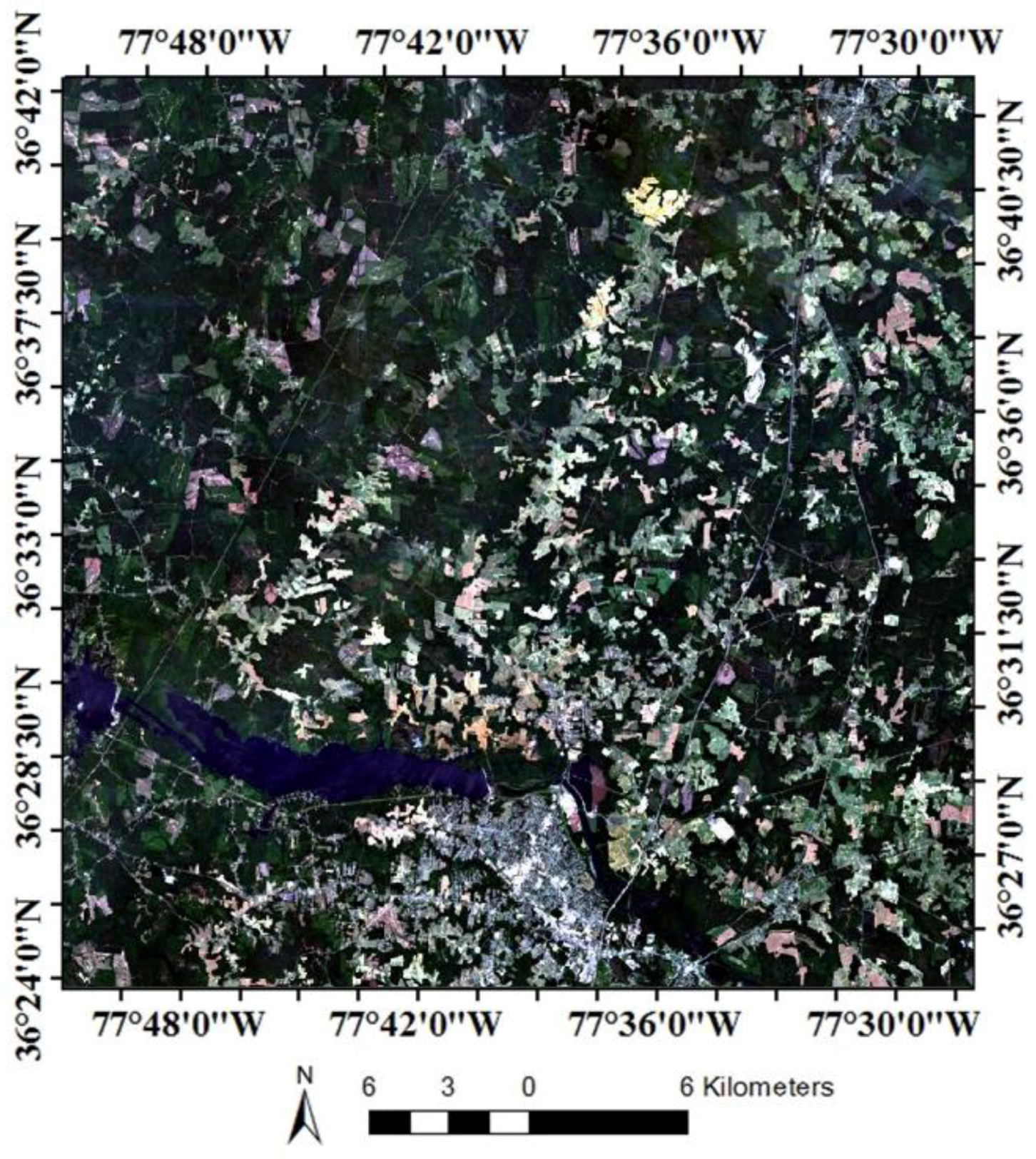
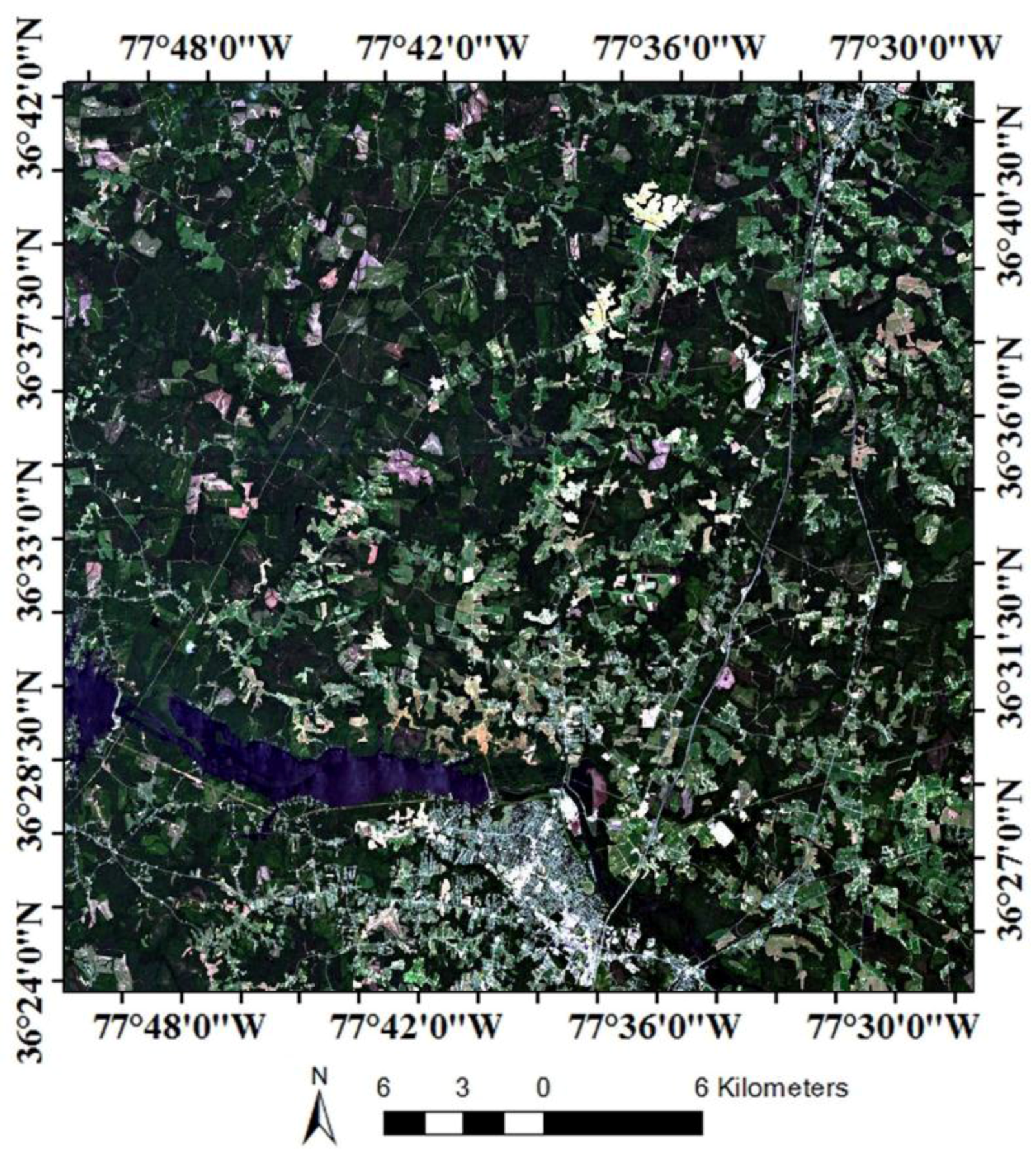
2.3. Study Area and Landsat-8 Datasets

One Landsat-8 OLI image of 015/035 (path/row) acquired on 13 July 2014 is identified and downloaded from the United States Geological Survey (USGS) website (http://earthexplorer.usgs.gov/). A sub-image of Landsat-8 is shown as a color composite of Band 4 as red, Band 3 as green, and Band 2 as blue (Figure 2). The image is 1000 (rows) × 1000 (columns) and it is centered at 36°33′17.64″N, 77°39′49.72″W. The area is around Roanoke Rapids, North Carolina (NC), USA. The LULC types are predominantly agriculture, forest, grassland, and water, as well as patches of developed areas.

Figure 2. A sub-image of Landsat-8 acquired on 13 July 2014 is shown as a color composite (Band 4 as red, Band 3 as green, and Band 2 as blue). Clouds as bright features are noticeable. The image is 1000 rows (30 km) by 1000 columns (30 km). The area is around Roanoke Rapids, NC.

Figure 2. A sub-image of Landsat-8 acquired on 13 July 2014 is shown as a color composite (Band 4 as red, Band 3 as green, and Band 2 as blue). Clouds as bright features are noticeable. The image is 1000 rows (30 km) by 1000 columns (30 km). The area is around Roanoke Rapids, NC.

3. Results and Discussions

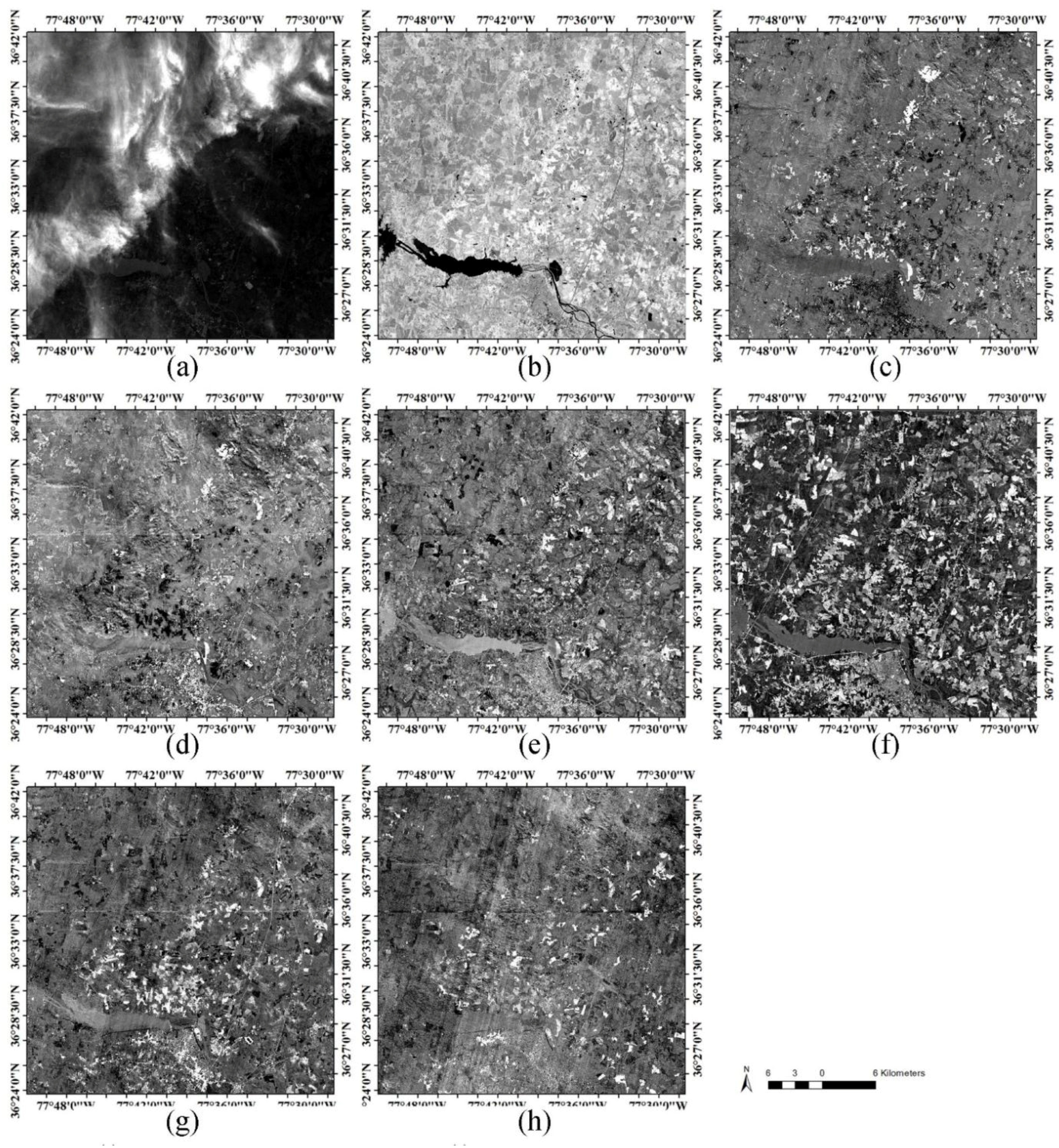
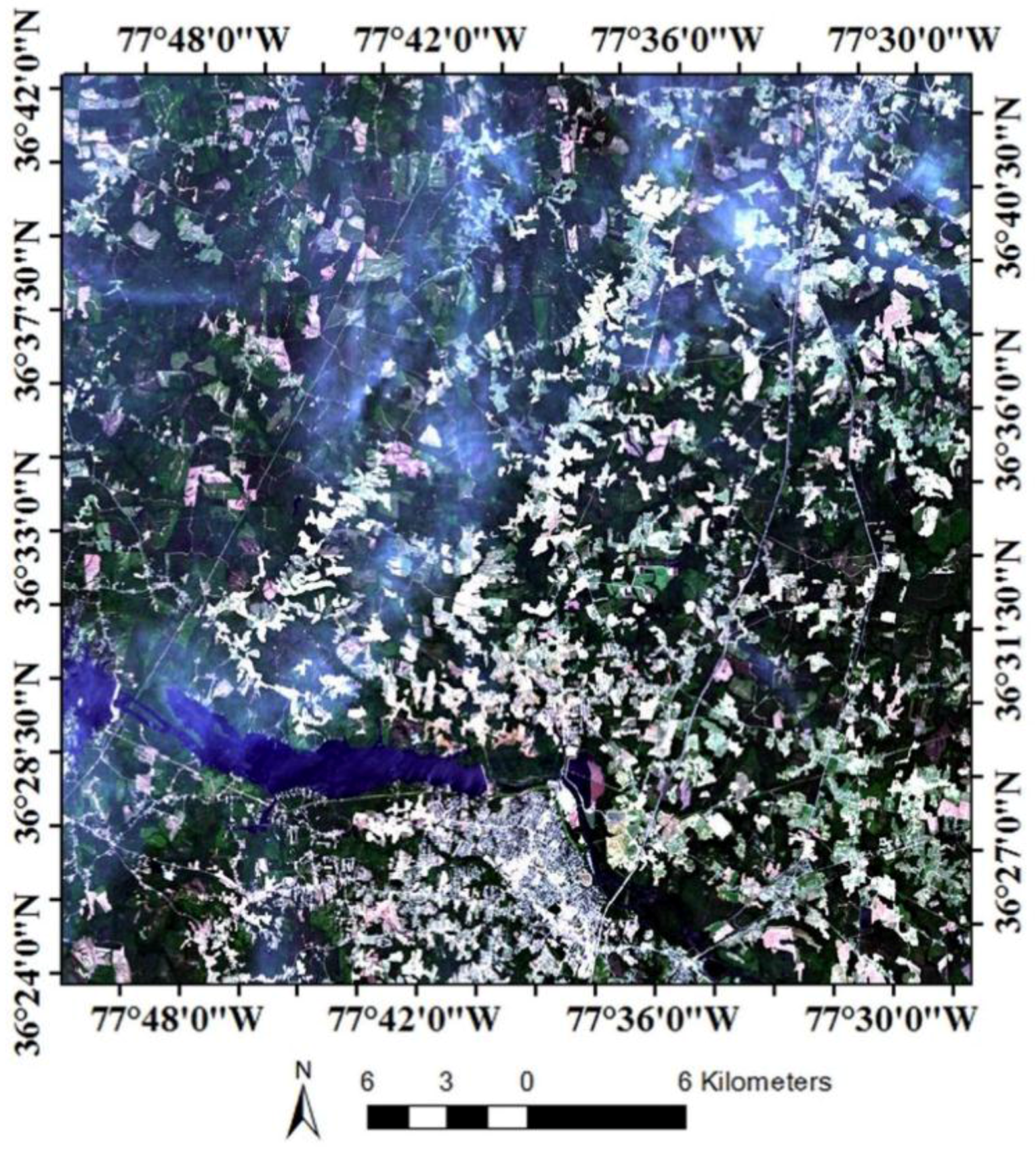
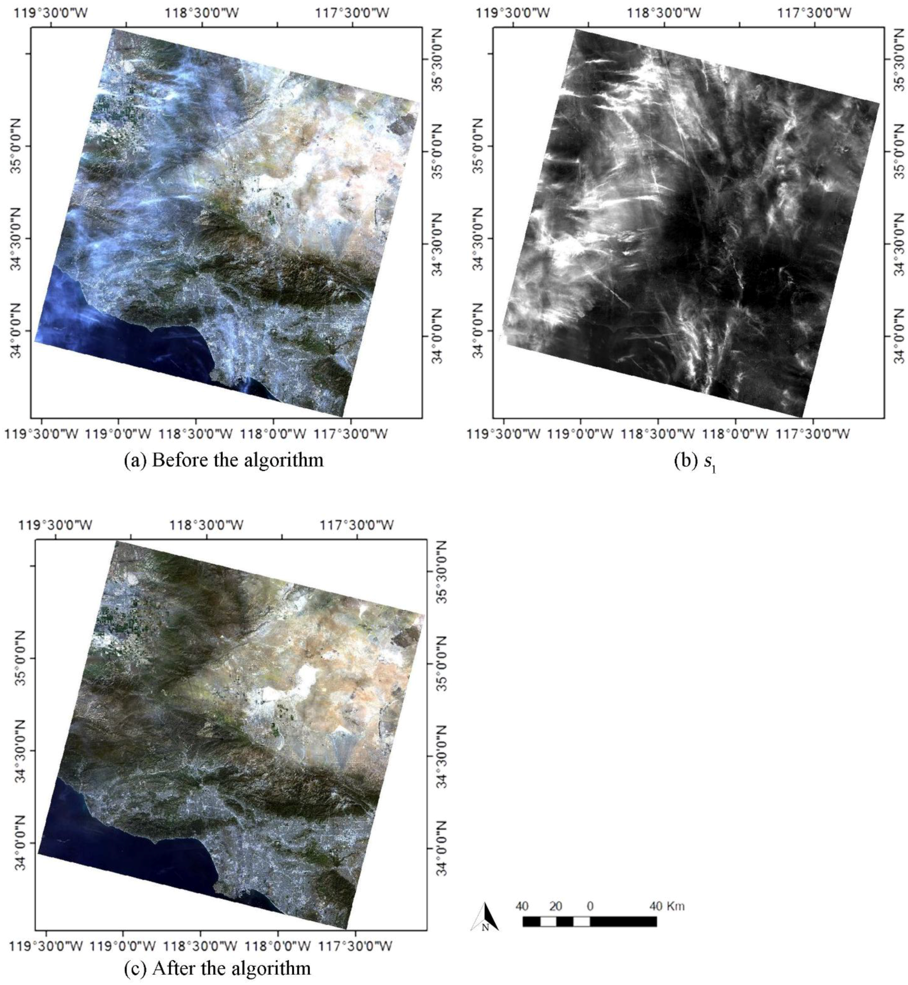
3.1. Cloud Correction

Inputting Bands 1–7 and 9 data into the FastICA algorithm, we obtained eight ICs (Figure 3). As stated previously, the first IC (Figure 3a) is considered as cloud component. Visually, the bright spatial patterns were similar to those of clouds in Figure 2. In addition to each IC, A and its elements were obtained (Table 1). The elements show relationships among Bands 1–7 and 9, and ICs, quantitatively. For example, of the coefficients of Band 9, s₁ had the largest value of 0.496 × 10⁻². The value was ~14 times larger than the second largest value (–0.036 × 10⁻²) of s₂, absolutely (Table 1). In the reference to Equation (4), ${\mathrm{\rho }}_{clou{d}_1}=a_{11}{s}_1=0.903\times {10}^{-2}\cdot s_1$, ${\mathrm{\rho }}_{clou{d}_2}=a_{21}{s}_1=0.795\times {10}^{-2}\cdot s_1$, …, and ${\mathrm{\rho }}_{clou{d}_7}=a_{71}{s}_1=-0.134\times {10}^{-2}\cdot s_1$.

Figure 3. (a–h) are first, second, …, and eighth independent components, respectively.

Figure 3. (a–h) are first, second, …, and eighth independent components, respectively.

Table 1. Coefficients (×10⁻²) of A.

	s1	s2	s3	s4	s5	s6	s7	s8
Band 1	0.903	0.394	0.321	–0.023	1.217	1.033	0.554	1.170
Band 2	0.795	0.635	0.426	0.025	1.248	1.209	0.662	1.211
Band 3	0.594	0.674	1.112	0.434	1.440	1.742	1.182	1.295
Band 4	0.542	1.398	1.046	1.028	1.972	2.497	1.132	1.371
Band 5	–0.870	–1.602	8.079	–0.240	–0.026	–1.267	–0.185	0.772
Band 6	–0.491	1.832	4.525	0.404	2.055	5.996	0.519	0.809
Band 7	–0.134	1.819	2.401	0.295	2.395	4.310	0.961	0.376
Band 9	0.496	–0.036	0.030	0.021	–0.019	–0.016	–0.011	–0.010

Table 1. Coefficients (×10⁻²) of A.

	s1	s2	s3	s4	s5	s6	s7	s8
Band 1	0.903	0.394	0.321	–0.023	1.217	1.033	0.554	1.170
Band 2	0.795	0.635	0.426	0.025	1.248	1.209	0.662	1.211
Band 3	0.594	0.674	1.112	0.434	1.440	1.742	1.182	1.295
Band 4	0.542	1.398	1.046	1.028	1.972	2.497	1.132	1.371
Band 5	–0.870	–1.602	8.079	–0.240	–0.026	–1.267	–0.185	0.772
Band 6	–0.491	1.832	4.525	0.404	2.055	5.996	0.519	0.809
Band 7	–0.134	1.819	2.401	0.295	2.395	4.310	0.961	0.376
Band 9	0.496	–0.036	0.030	0.021	–0.019	–0.016	–0.011	–0.010

Next, the cloud removed image has been obtained using Equation (5). A color composite (Band 4 as red, Band 3 as green, and Band 1 as blue) is shown in Figure 4. In comparison with the before image (Figure 2), clouds have been removed visually. Ground features where there are no clouds remain. Overall, the cloud removal was encouraging. The quantitative assessment is carried out next.

Figure 4. Landsat-8 OLI data acquired on 13 July 2014 after the removal of clouds. The color composite is with Band 4 as red, Band 3 as green, and Band 2 as blue.

Figure 4. Landsat-8 OLI data acquired on 13 July 2014 after the removal of clouds. The color composite is with Band 4 as red, Band 3 as green, and Band 2 as blue.

3.2. Assessment

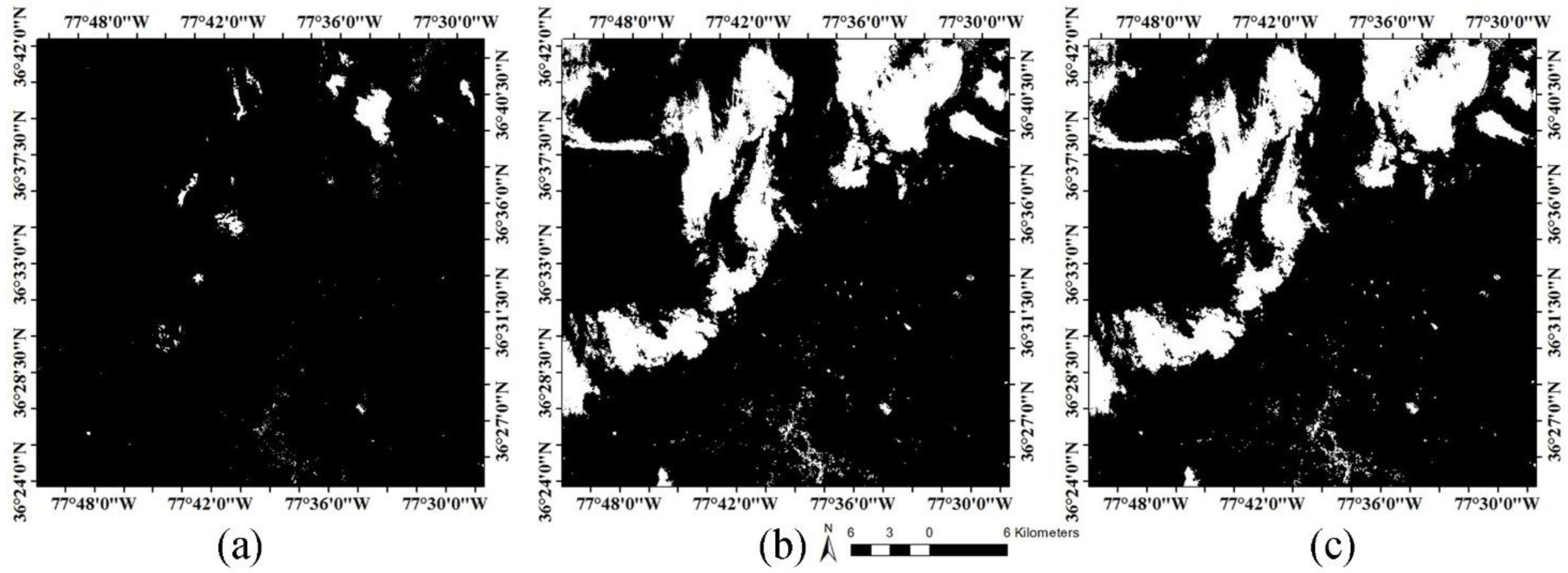
3.2.1. Cloud and Cloud-Free Masks

Of the study area, the numbers of pixels with 10 and 11 of bits of 12 and 13, and 10 and 11 of bits of 14 and 15 in QA band were 13,007 and 1251, respectively. The union of both numbers was 14,246. Figure 5a was the mask derived from QA Band and was shown as a binary image (cloud pixels: white, and non-cloud pixels: black). Because the number was small, the QA band might not identify all clouds in the study area. Then, the image segmentation method [30] was used. The number of cloud-covered pixels delineated by the segmentation method was 188,975 (Figure 5b). The increase of cloud-covered pixels could be attributed to different methods for the cloud delineation. However, the variation in the number of cloud-covered pixels should not affect the development of the cloud removal algorithm because the mask was only used to assist the evaluation of the algorithm in the cloud-covered and cloud-free areas. Furthermore, our intent was to use the algorithm for an entire input image. After the union of the cloud pixels derived from the QA band and the segmentation method, the number of total cloud-covered pixels was 189,054. The percentage of cloudy pixels was about 18.9%. Figure 5c was the mask after the union of Figure 5a,b.

Figure 5. Cloud/non-cloud masks shown as a binary image with cloud being white and non-cloud as black. (a) The mask derived from QA Band, (b) the mask derived from the segmentation method, and (c) The mask after logical union operation of (a) and (b). (c) is used in the algorithm assessment.

Figure 5. Cloud/non-cloud masks shown as a binary image with cloud being white and non-cloud as black. (a) The mask derived from QA Band, (b) the mask derived from the segmentation method, and (c) The mask after logical union operation of (a) and (b). (c) is used in the algorithm assessment.

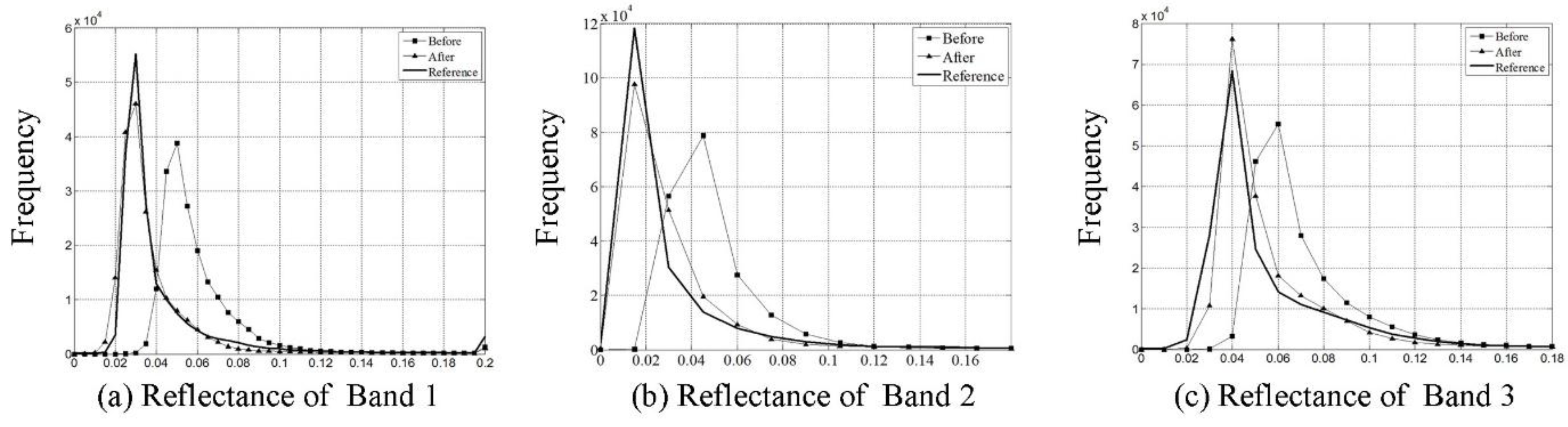
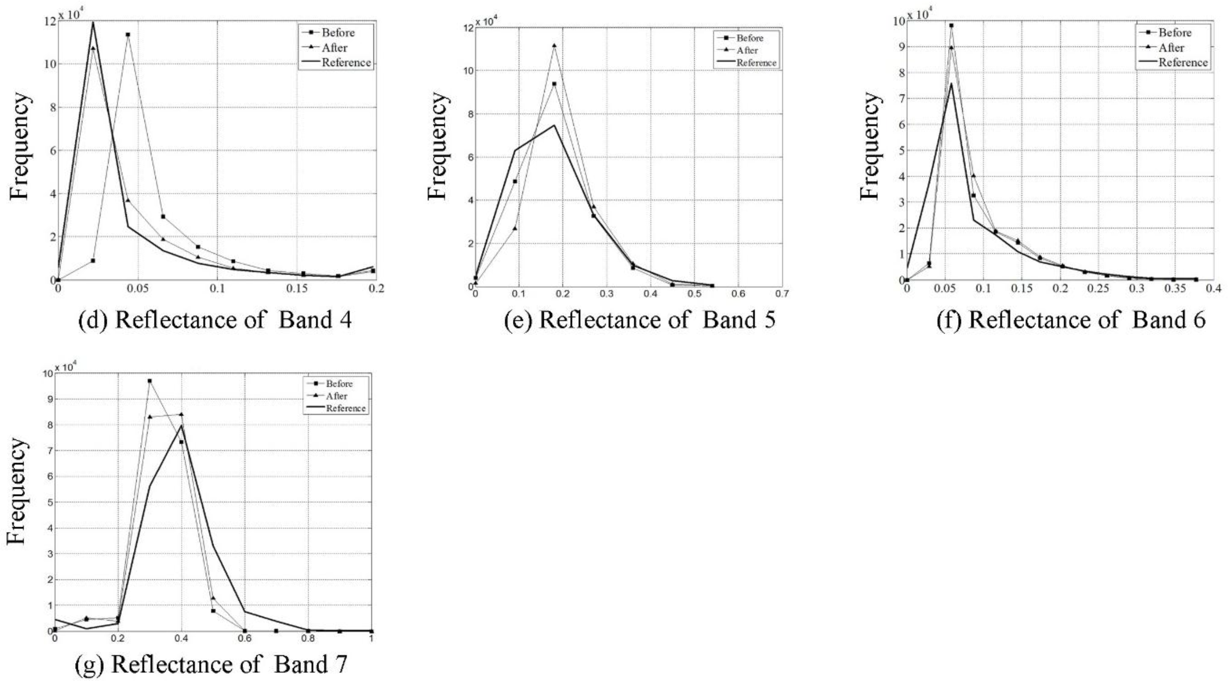
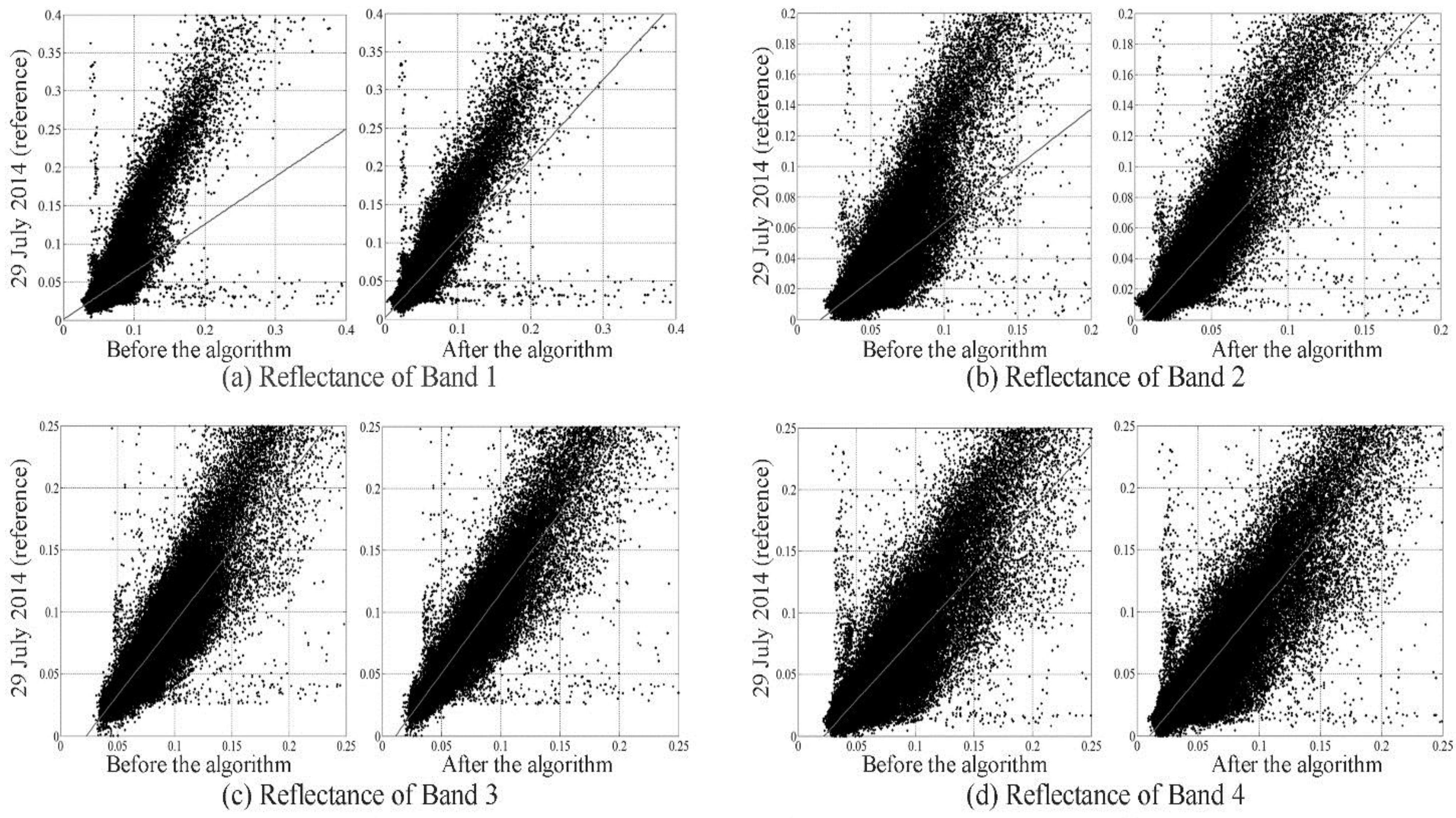
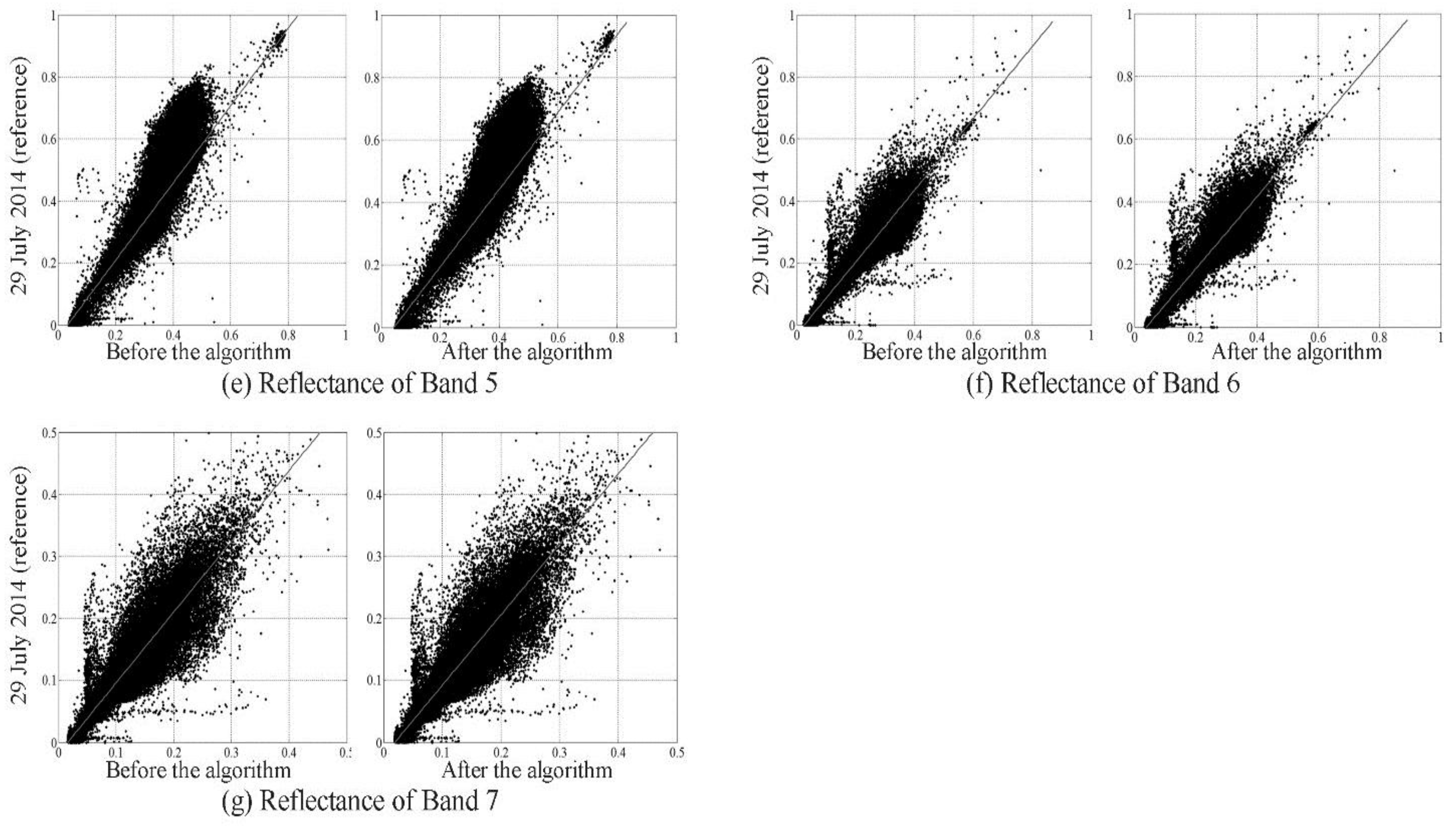
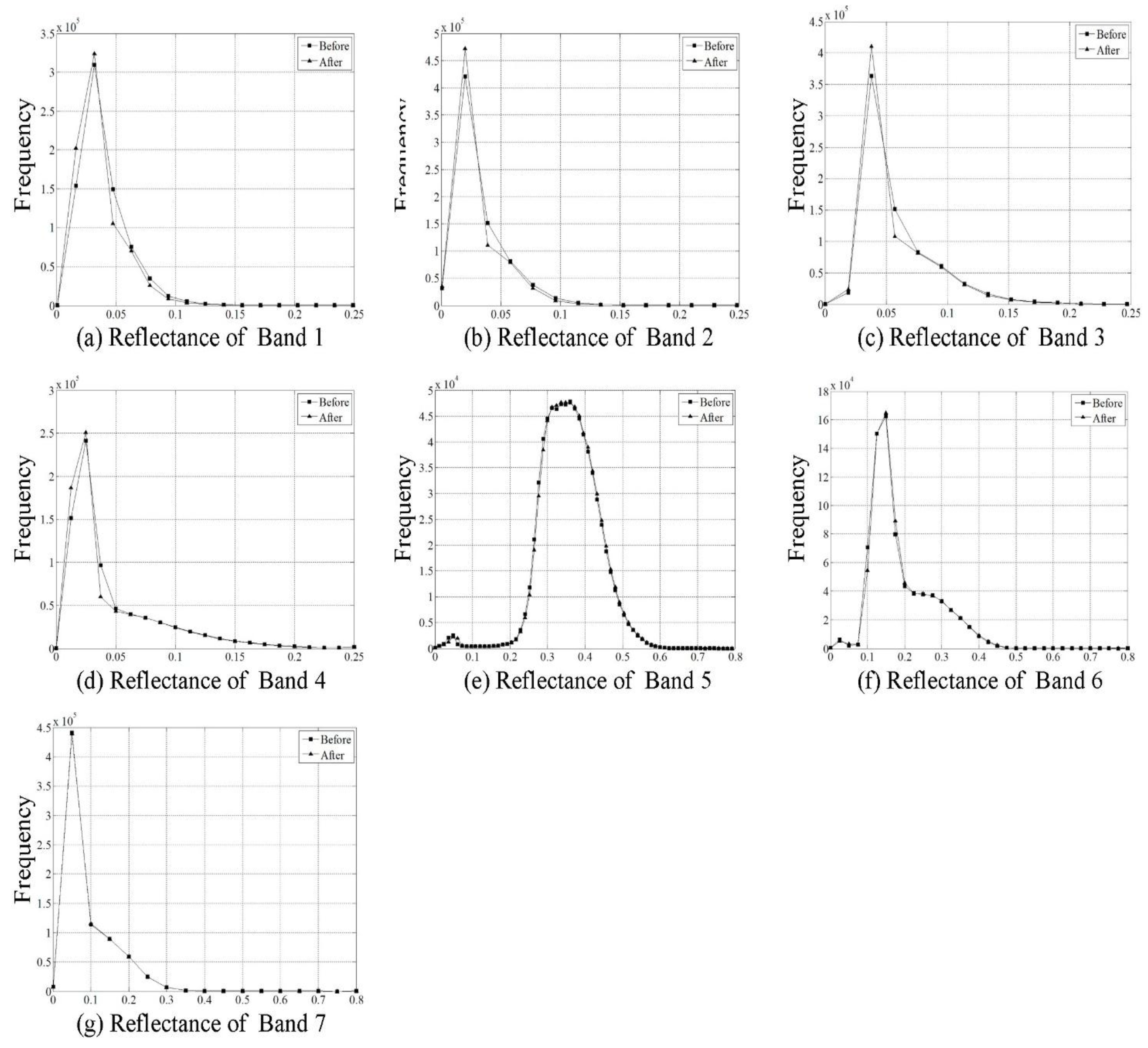
3.2.2. Assessment in Cloud-Covered Areas

Due to the constant spatial and temporal variations of clouds, the verification of the developed algorithm is done through comparison of the 13 July 2014 image before and after the cloud removal with a cloud-free image as reference. To do so, we assume that surface reflectance from cloud-free areas (from the 13 July 2014 image and the reference image) should be the same. With the solo Landsat-8, the best possibility candidate is another dataset that is 16 days before or after the (current) acquisition time. Thus, we are limited with the images acquired on 28 June 2014 and 29 July 2014. Fortunately, the image acquired on 29 July 2014 was cloud-free in our study area. Thus, the image was selected as the reference image (Figure 6).

After identifying cloud-covered pixels from Bands 1–7 with the cloud mask (Figure 5c), we extracted the reflectance values from the pixels of the 13 July 2014 image before and after the cloud removal algorithm, and from the same pixels of the reference image. Histograms showing the reflectance values of the cloudy pixels before and after the algorithm were given in Figure 7. After the algorithm, the histogram curve moved closer to that of the reference image, band-by-band. Therefore, the movement of each histogram curve revealed the effectiveness of the algorithm to remove clouds.

To evaluate the performance of the algorithm further, we analyzed scatterplots of the reflectance values of the cloud-covered pixels paired by the 13 July 2014 image before the algorithm versus the 29 July 2014 image, and by the 13 July 2014 image after the algorithm versus the 29 July 2014 image. The scatterplots of seven bands were given (Figure 8). Per band, points of the scatterplots moved toward the 1:1 ratio line after the algorithm. The movement suggested that the algorithm was working properly. The least-squared linear fit was performed. The slope, intercept, and R² were summarized in Table 2. Sixteen out of the total 21 cases, the slope moved closer to 1.0, the intercept to 0.0, and R² to 1.0 after applying the algorithm. For instance, the slope increased from 0.624 to 1.038, the intercept was the same as 0.001, and the R² increased from 0.965 to 0.977 in Band 1. Even though there were five exceptional cases (as italicized in the table), the results should be satisfactory overall.

Figure 6. The reference image of the study area shown as a color composite with Bands 4 as red, Band 3 as green, and Band 2 as blue. The image was acquired on 29 July 2014.

Figure 6. The reference image of the study area shown as a color composite with Bands 4 as red, Band 3 as green, and Band 2 as blue. The image was acquired on 29 July 2014.

Table 2. Coefficients of linear regression analyses of Bands 1–7 before and after the cloud removal in comparison with the reference image (Five exceptional cases are italicized).

	Slope		Intercept		R2
	Before	After	Before	After	Before	After
Band 1	0.624	1.038	0.001	0.001	0.965	0.977
Band 2	0.745	1.095	–0.012	–0.005	0.968	0.982
Band 3	1.182	1.303	–0.027	–0.015	0.963	0.983
Band 4	1.034	1.178	–0.023	–0.012	0.976	0.989
Band 5	1.249	1.238	–0.042	–0.054	0.922	0.933
Band 6	1.160	1.151	–0.045	–0.030	0.967	0.955
Band 7	1.143	1.138	–0.023	–0.019	0.974	0.969

Table 2. Coefficients of linear regression analyses of Bands 1–7 before and after the cloud removal in comparison with the reference image (Five exceptional cases are italicized).

	Slope		Intercept		R2
	Before	After	Before	After	Before	After
Band 1	0.624	1.038	0.001	0.001	0.965	0.977
Band 2	0.745	1.095	–0.012	–0.005	0.968	0.982
Band 3	1.182	1.303	–0.027	–0.015	0.963	0.983
Band 4	1.034	1.178	–0.023	–0.012	0.976	0.989
Band 5	1.249	1.238	–0.042	–0.054	0.922	0.933
Band 6	1.160	1.151	–0.045	–0.030	0.967	0.955
Band 7	1.143	1.138	–0.023	–0.019	0.974	0.969

Figure 7. Histograms of reflectance values for the cloud-covered pixels in 13 July 2014 image before and after the algorithm, and for the corresponding pixels of the reference image acquired on 29 July 2014. (a) Band 1; (b) Band 2; (c) Band 3; (d) Band 4; (e) Band 5; (f) Band 6; (g) Band 7.

Figure 7. Histograms of reflectance values for the cloud-covered pixels in 13 July 2014 image before and after the algorithm, and for the corresponding pixels of the reference image acquired on 29 July 2014. (a) Band 1; (b) Band 2; (c) Band 3; (d) Band 4; (e) Band 5; (f) Band 6; (g) Band 7.

Figure 8. Scatterplots of Bands 1–7 for cloud-covered pixels on the 13 July 2014 image. The 13 July 2014 image before the cloud removal (before) vs. the 29 July 2014 image (as reference). The 13 July 2014 image after the cloud removal (after) vs. the 29 July 2014 image. (a–g) are Bands 1–7, respectively.

Figure 8. Scatterplots of Bands 1–7 for cloud-covered pixels on the 13 July 2014 image. The 13 July 2014 image before the cloud removal (before) vs. the 29 July 2014 image (as reference). The 13 July 2014 image after the cloud removal (after) vs. the 29 July 2014 image. (a–g) are Bands 1–7, respectively.

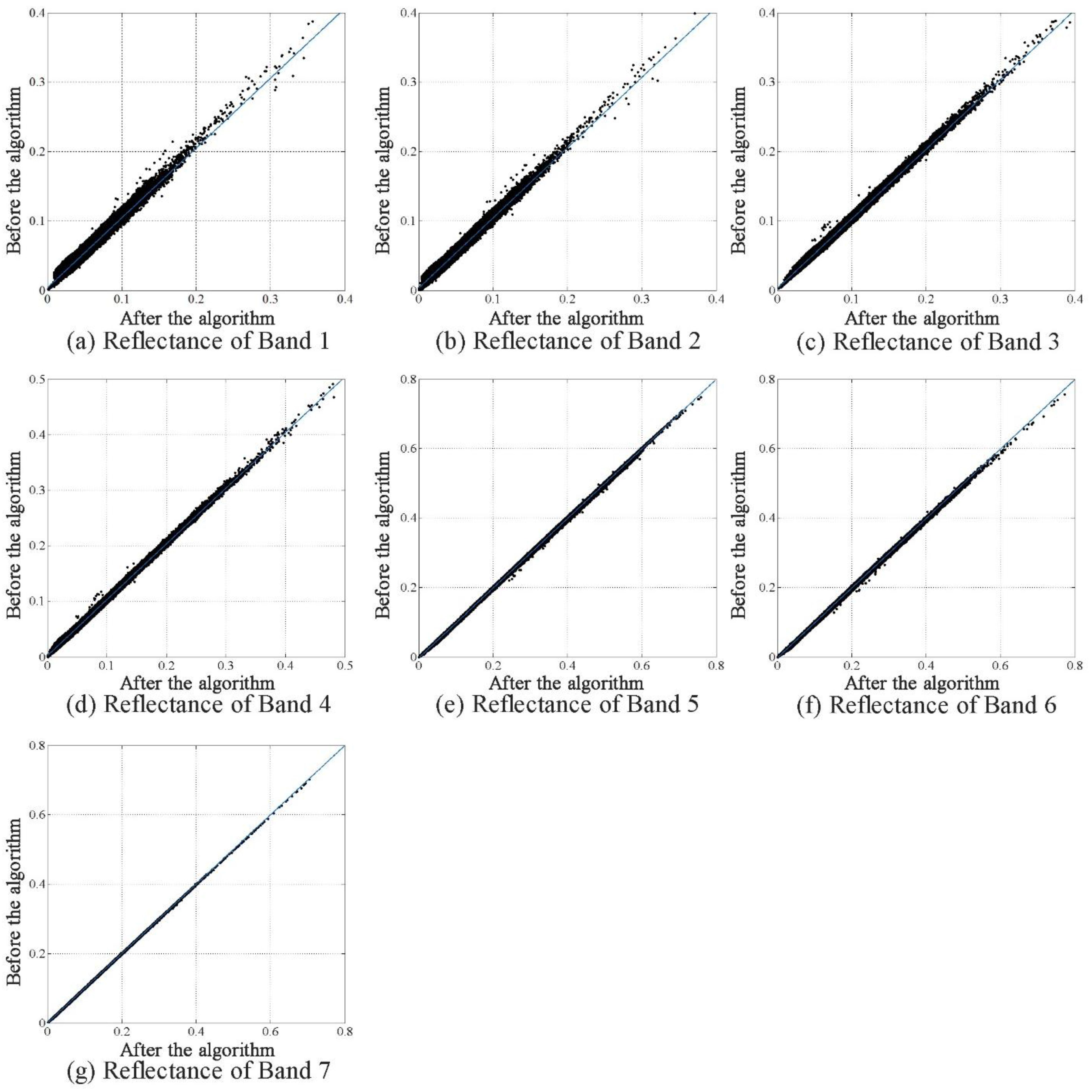
3.2.3. Assessment in Cloud-Free Areas

Since the ICA algorithm is applied to the entire image, we need to know whether the algorithm alters the reflectance value of each cloud-free pixel. In the assessment, the algorithm was applied to cloud-free pixels of the 13 July 2014 image. Then, the results were compared to the cloud-free pixels of the original 13 July 2014 image. If the algorithm is deemed valid, it should have none or a minimum impact on the reflectance values for the pixels. Histograms of reflectance values before and after the algorithm were given in Figure 9. Of each plot, both (before and after) curves were almost identical. This was especially true for the before and after curves of Band 5, Band 6, or Band 7. They were overlapped entirely. A very small variation was observed for the histogram curves after the algorithm was applied to Bands 1–4. Scatterplots of Bands 1–7 are shown in Figure 10. Almost all pixels were clustered around the 1:1 ratio line. Thus, the algorithm had little effect on the reflectance values from cloud-free pixels of Bands 1–7. Finally, the slope, intercept, and R² of linear regression analyses were tabulated (Table 3). Overall, the slope, intercept, and R² were close to 1.0, 0.0, and 1.0, respectively. Therefore, the algorithm did not change the reflectance values from the cloud-free pixels noticeably.

Table 3. Linear regression analyses of cloud-free pixels before and after the algorithm.

	Slope	Intercept	R2
Band 1	1.007	0.004	0.910
Band 2	1.007	0.003	0.944
Band 3	1.001	0.003	0.984
Band 4	1.002	0.003	0.992
Band 5	1.002	–0.003	0.999
Band 6	1.002	–0.003	0.998
Band 7	1.000	–0.001	0.999

Table 3. Linear regression analyses of cloud-free pixels before and after the algorithm.

	Slope	Intercept	R2
Band 1	1.007	0.004	0.910
Band 2	1.007	0.003	0.944
Band 3	1.001	0.003	0.984
Band 4	1.002	0.003	0.992
Band 5	1.002	–0.003	0.999
Band 6	1.002	–0.003	0.998
Band 7	1.000	–0.001	0.999

Figure 9. Histograms of reflectance values for cloud-free pixels before and after the algorithm. (a) Band 1; (b) Band 2; (c) Band 3; (d) Band 4; (e) Band 5; (f) Band 6; (g) Band 7.

Figure 9. Histograms of reflectance values for cloud-free pixels before and after the algorithm. (a) Band 1; (b) Band 2; (c) Band 3; (d) Band 4; (e) Band 5; (f) Band 6; (g) Band 7.

Figure 10. Scatterplots of cloud-free pixels before and after the algorithm. (a–g) are Bands 1–7, respectively.

Figure 10. Scatterplots of cloud-free pixels before and after the algorithm. (a–g) are Bands 1–7, respectively.

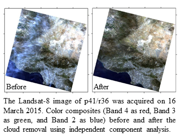
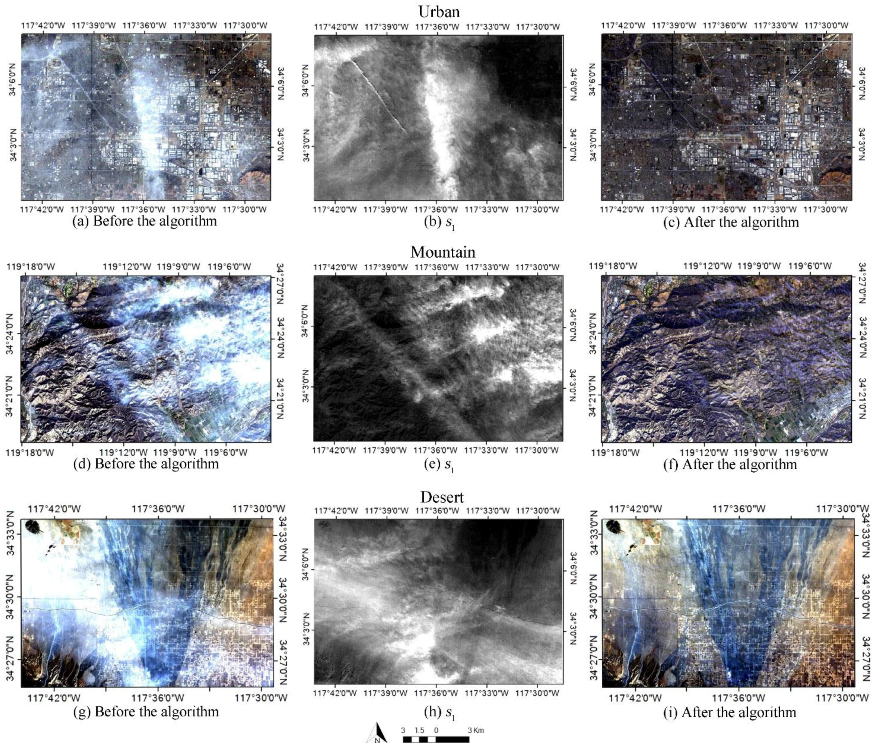
3.3. Applicability to Other LULC Types and to an Entire Landsat-8 Image

To assess the applicability of the algorithm to various types of LULC types, we downloaded another Landsat-8 OLI image acquired on 8 January 2014. The path and row numbers were 41, and 36, respectively. The area covered by the image was near Los Angeles, California (CA), USA. In the scene, the typical LULC types were urban, desert, cropland land, mountain, vegetation, and ocean. Three subimages were extracted. Each subimage consisted of 500 (rows) × 750 (columns) or 15.0 km × 22.5 km. Figure 11a centered at 34°4′27.30″N and 117°35′52.16″W was dominated by urban. The area was near Rancho Cucamonga, CA. Clouds were scattered within the entire subimage. The cloud component was shown in Figure 11b. Figure 11c was the cloud-removed subimage. Clearly, clouds were removed, but ground features underneath clouds remained and were properly revealed. The mean values before and after the algorithm were tabulated in Table 4.

Figure 11. Three subimages extracted from the image of p41/r36 of Landsat-8 OLI data acquired on 8 January 2014. (a) The original urban image. (b) The cloud component of the image. (c) The image after the algorithm. (d) The original mountainous image. (e) The cloud component of the image. (f) The image after the algorithm. (g) The original desert image. (h) The cloud component of the image. (i) The image after the algorithm. (a), (c), (d), (f), (g), and (i) are the color composites with Band 4 as red, Band 3 as green, and Band 2 as blue, respectively. (b), (e), and (h) are in gray scale.

Figure 11. Three subimages extracted from the image of p41/r36 of Landsat-8 OLI data acquired on 8 January 2014. (a) The original urban image. (b) The cloud component of the image. (c) The image after the algorithm. (d) The original mountainous image. (e) The cloud component of the image. (f) The image after the algorithm. (g) The original desert image. (h) The cloud component of the image. (i) The image after the algorithm. (a), (c), (d), (f), (g), and (i) are the color composites with Band 4 as red, Band 3 as green, and Band 2 as blue, respectively. (b), (e), and (h) are in gray scale.

Mountains and valleys near Ventura, CA were the predominate ground features in Figure 11d that is centered at 34°22′53.34″N and 119°10′49.31″W. Cloud cover was noted on the east. After applying the algorithm, the cloud component was derived (Figure 11e). Almost all clouds were removed (Figure 11f). Decreases in mean values after the algorithm were observed (Table 4).

Figure 11g showed desert where dry bare soil is the major LULC type. The subimage was centered at 34°29′43.56″N and 117°36′38.81″W and was near Pinon Hill, CA. Clouds mainly existed in the west, south, and southeast. After the algorithm, we identified the cloud component (Figure 11h), and removed the clouds (Figure 11i). The mean values before and after the algorithm were also tabulated in Table 4.

Table 4. Mean values of three subimages before and after the algorithm.

	Urban		Mountain		Desert
	Before	After	Before	After	Before	After
Band 1	0.205	0.172	0.181	0.156	0.188	0.176
Band 2	0.189	0.155	0.160	0.135	0.178	0.166
Band 3	0.167	0.134	0.133	0.108	0.173	0.161
Band 4	0.168	0.135	0.131	0.106	0.190	0.178
Band 5	0.222	0.175	0.206	0.170	0.238	0.221
Band 6	0.183	0.154	0.229	0.207	0.257	0.246
Band 7	0.154	0.130	0.173	0.155	0.225	0.216

Table 4. Mean values of three subimages before and after the algorithm.

	Urban		Mountain		Desert
	Before	After	Before	After	Before	After
Band 1	0.205	0.172	0.181	0.156	0.188	0.176
Band 2	0.189	0.155	0.160	0.135	0.178	0.166
Band 3	0.167	0.134	0.133	0.108	0.173	0.161
Band 4	0.168	0.135	0.131	0.106	0.190	0.178
Band 5	0.222	0.175	0.206	0.170	0.238	0.221
Band 6	0.183	0.154	0.229	0.207	0.257	0.246
Band 7	0.154	0.130	0.173	0.155	0.225	0.216

Finally, to assess the efficiency of the algorithm, we applied it to process an entire Landsat 8 OLI image of p41/r36. The image was acquired on 16 March 2015. The image was shown in Figure 12a as a color composite with Band 4 as red, Band 3 as green, and Band 2 as blue. The image consisted of 6560 rows (along the satellite flying direction) by 6330 columns (perpendicular to the flight direction) of data. It was about 196.8 km along the flight direction, and 189.9 km in cross flight direction. The city of Los Angeles was located near the south and southeast. Clouds existed mainly on the west and south. The cloud component was given in Figure 12b. As an example, the result was shown as a color composite with Band 4 as red, Band 3 as green, and Band 2 as blue (Figure 12c). Clouds were clearly removed. The process time was 42 minutes with an Intel^® Core^TM i5-3470 CPU at 3.20 GHz and 3.20 GHz, and an 8-GB RAM under 64-bit Windows 7 operating system. Thus, the algorithm was able to process an entire Landsat-8 scene efficiently.

4. Conclusions

An approach to remove clouds using the independent component analysis (ICA) coupled with cirrus band (Band 9) was developed for Landsat 8 OLI data. With the input of Bands 1–7 and 9, eight independent components were generated. Then, based on the weight value on each component from Band 9 data, the cloud related component was identified. After the subtraction of the cloud reflectance, the cloud corrected result was achieved.

Visually, clouds disappeared after the algorithm in five locations where difference land use and land cover types existed. In the quantitative assessment of the algorithm, changes of histogram curves, referred to a cloud-free (reference) image, indicated the validity of the algorithm. For pixels of cloud-covered areas, the scatterplot and linear regression of reflectance values of one band before the algorithm versus the corresponding band of the reference image were generated. Similarly, in cloud-free areas, the scatterplot and linear regression of one band before and after the algorithm were produced. Band-by-band, both types of the scatterplots, and the regression equations were evaluated. The results were satisfactory. When the algorithm was applied to an entire Landsat 8 OLI image, the process time was 42 minutes with an Intel^® Core^TM i5-3470 CPU at 3.20 GHz and 3.20 GHz, and an 8-GB RAM under 64-bit Windows 7 operating system. Thus, the algorithm was able to remove clouds efficiently as well.

Figure 12. (a) The Landsat image of p41/r36 was acquired on 16 March 2015; (b) The cloud component, s₁ in gray scale; (c) The Landsat image after the algorithm. Color composites before (a) and after (b) the algorithm were with Band 4 as red, Band 3 as green, and Band 2 as blue.

Figure 12. (a) The Landsat image of p41/r36 was acquired on 16 March 2015; (b) The cloud component, s₁ in gray scale; (c) The Landsat image after the algorithm. Color composites before (a) and after (b) the algorithm were with Band 4 as red, Band 3 as green, and Band 2 as blue.

Before ending this article, we would argue the algorithm assessment using the reference dataset. Because of the spatiotemporal variability of clouds in general, the approach using the in situ measurement traditionally done in remote sensing studies is impossible. An alternative approach is to find a reference image from the same remote sensor, and the image is cloud free within the study area. Due to the solo Landsat-8, possible candidates for the reference images include the image acquired 16 days before or after the evaluating image, and the image acquired near anniversary dates (of the evaluating image). In addition, if the study area is near the edge such as on the west side and is small enough within the overlapped areas of the current path and west-adjacent path, an interval of seven days is possible. Nevertheless, reflectance characteristics from ground targets can vary temporally. In addition, the reference image is usable only if the study area is cloud free. Therefore, the outcome in assessment can be greatly affected by the selection and use of the reference image(s).

References

1. U.S. Geological Survey. Landsat—A global Land-Imaging Mission: U.S. Geological Survey fact sheet 2012–3072. Available online: http://pubs.usgs.gov/fs/2012/3072/ (accessed on 15 August 2015).
2. Xu, M.; Jia, X.; Pickering, M. Automatic cloud removal for Landsat 8 OLI images using cirrus band. In Proceedings of the IEEE International Geoscience and Remote Sensing Symposium, Quebec City, QC, Canada, 13–18 July 2014; pp. 2511–2514.
3. Shen, Y.; Wang, Y.; Lv, H.; Li, H. Removal of thin clouds using cirrus and QA bands of Landsat 8. Photogramm. Eng. Remote Sens. 2015, 81, 721–731. [Google Scholar] [CrossRef]
4. Goodwin, N.R.; Collett, L.J.; Denham, R.J.; Flood, N.; Tindall, D. Cloud and cloud shadow screening across Queensland, Australia: An automated method for Landsat TM/ETM+ time series. Remote Sens. Environ. 2013, 134, 50–65. [Google Scholar] [CrossRef]
5. Chanda, B.; Majumder, D.D. An iterative algorithm for removing the effect of thin cloud cover from LANDSAT imagery. Math. Geol. 1991, 23, 853–860. [Google Scholar] [CrossRef]
6. Shen, H.; Li, H.; Qian, Y.; Zhang, L.; Yuan, Q. An effective thin cloud removal procedure for visible remote sensing Images. ISPRS J. Photogramm. Remote Sens. 2014, 96, 224–235. [Google Scholar] [CrossRef]
7. Tseng, D.C.; Tseng, H.T.; Chien, C.L. Automatic cloud removal from multi-temporal SPOT images. Appl. Math. Comput. 2008, 205, 584–600. [Google Scholar] [CrossRef]
8. Cheng, Q.; Shen, H.; Zhang, L.; Yuan, Q.; Zeng, C. Cloud removal for remotely sensed images by similar pixel replacement guided with a spatio-temporal MRF model. ISPRS J. Photogramm. Remote Sens. 2014, 92, 54–68. [Google Scholar] [CrossRef]
9. Jin, S.; Homer, C.G.; Yang, L.; Xian, G.; Fry, J.; Danielson, P.; Townsend, P.A. Automated cloud and shadow detection and filling using two-date Landsat imagery in the USA. Int. J. Remote Sens. 2013, 34, 1540–1560. [Google Scholar] [CrossRef]
10. Liu, J.; Wang, X.; Chen, M.; Liu, S.G.; Zhou, X.R.; Shao, Z.F.; Liu, P. Thin cloud removal from single satellite images. Opt. Express 2014, 22, 618–632. [Google Scholar] [CrossRef] [PubMed]
11. Earth Observation Portal. Available online: https://directory.eoportal.org/web/eoportal/directory (accessed on 15 August 2015).
12. Zhang, Y.; Guindon, B.; Cihlar, J. An image transform to characterize and compensate for spatial variations in thin cloud contamination of Landsat images. Remote Sens. Environ. 2002, 82, 173–187. [Google Scholar] [CrossRef]
13. Kauth, R.J.; Thomas, G.S. The Tasseled Cap—A graphic description of the spectral-temporal development of agricultural crops as seen in Landsat. In Proceedings of the Landsat Symposium on Machine Processing of Remotely Sensed Data, West Lafayette, IN, USA, 29 June–1 July 1976; pp. 41–51.
14. Li, H.; Zhang, L.; Shen, H. A principal component based haze masking method for visible images. IEEE Geosci. Remote Sens. Lett. 2013, 11, 975–979. [Google Scholar] [CrossRef]
15. Crist, E.P.; Cicone, R.C. A physically-based transformation of Thematic Mapper data—The TM Tasselled Cap. IEEE Trans. Geosci. Remote Sens. 1984, 22, 256–263. [Google Scholar] [CrossRef]
16. Lavreau, J. De-Hazing Landsat thematic mapper images. Photogramm. Eng. Remote Sens. 1991, 57, 1297–1302. [Google Scholar]
17. Baig, M.H.A.; Zhang, L.; Tong, S.; Tong, Q. Derivation of a Tasselled Cap transformation based on Landsat 8 at-satellite reflectance. Remote Sens. Lett. 2014, 5, 423–431. [Google Scholar] [CrossRef]
18. Liu, Q.; Liu, G.; Huang, C.; Xie, C. Comparison of Tasselled Cap transformations based on the selective bands of Landsat 8 OLI TOA reflectance images. IEEE Trans. Geosci. Remote Sens. 2015, 36, 417–441. [Google Scholar] [CrossRef]
19. Miguel, M.; Carlos, J.G.; Horacio, G.; Ramón, G. Independent component analysis for cloud screening of Meteosat images. In Artificial Neural Nets Problem Solving Methods: 7th International Work-Conference on Artificial and Natural Neural Networks Proceedings, Part II; Springer: Berlin/Heidelberg, Germany, 2003; Volume 2687, pp. 551–558. [Google Scholar]
20. Unger, H.; Zeevi, Y.Y. Blind separation of a dynamic image source from superimposed reflections. Proc. SPIE 2005, 5888. [Google Scholar] [CrossRef]
21. Du, H.; Wang, Y.; Chen, Y. Studies on cloud detection of atmospheric remote sensing image using ICA algorithm. In Proceedings of the 2nd International Congress on Image and Signal Processing, Tianjin, China, 17–19 October 2009; pp. 1–4.
22. Hyvärinen, A. Fast and robust fixed-point algorithms for independent component analysis. IEEE Trans. Neural Netw. 1999, 10, 626–634. [Google Scholar] [CrossRef] [PubMed]
23. Hyvärinen, A.; Oja, E. Independent component analysis: algorithms and applications. Neural Netw. 2000, 13, 411–430. [Google Scholar] [CrossRef]
24. Ozdogan, M. The spatial distribution of crop types from MODIS data: Temporal unmixing using Independent Component Analysis. Remote Sens. Environ. 2010, 114, 1190–1204. [Google Scholar] [CrossRef]
25. Gao, B.; Yang, P.; Han, W.; Li, R.; Wiscombe, W.J. An algorithm using visible and 1.38-μm channels to retrieve cirrus cloud reflectances from aircraft and satellite data. IEEE Trans. Geosci. Remote Sens. 2002, 40, 1659–1668. [Google Scholar]
26. Ji, C.Y. Haze reduction from the visible bands of Landsat TM and ETM+ images over a shallow water reef environment. Remote Sens. Environ. 2008, 112, 1773–1783. [Google Scholar] [CrossRef]
27. Li, C.F.; Yin, J.Y. Variational Bayesian independent component analysis-support vector machine for remote sensing classification. Comput. Elect. Eng. 2013, 39, 717–726. [Google Scholar] [CrossRef]
28. Gao, B.; Li, R. Removal of thin cirrus scattering effects for remote sensing of ocean color from space. IEEE Geosci. Remote Sens. Lett. 2012, 9, 972–976. [Google Scholar]
29. U.S. Geological Survey. Landsat 8 Quality Assessment band. Available online: https://landsat.usgs.gov/L8QualityAssessmentBand.php (accessed on 15 August 2015).
30. Zhu, Z.; Woodcock, C.E. Object-based cloud and cloud shadow detection in Landsat imagery. Remote Sens. Environ. 2012, 118, 83–94. [Google Scholar] [CrossRef]