Abstract
The Shuttle Radar Topography Mission (SRTM) digital elevation model (DEM) is one of the most complete and frequently used global-scale DEM products in various applications. However, previous studies have shown that the SRTM DEM is systematically higher than the actual land surface in vegetated mountain areas. The objective of this study is to propose a procedure to calibrate the SRTM DEM over large vegetated mountain areas. Firstly, we developed methods to estimate canopy cover from aerial imagery and tree height from multi-source datasets (i.e., field observations, airborne light detection and ranging (LiDAR) data, Geoscience Laser Altimeter System (GLAS) data, Landsat TM imagery, climate surfaces, and topographic data). Then, the airborne LiDAR derived DEM, covering ~5% of the study area, was used to evaluate the accuracy of the SRTM DEM. Finally, a regression model of the SRTM DEM error depending on tree height, canopy cover, and terrain slope was developed to calibrate the SRTM DEM. Our results show that the proposed procedure can significantly improve the accuracy of the SRTM DEM over vegetated mountain areas. The mean difference between the SRTM DEM and the LiDAR DEM decreased from 12.15 m to −0.82 m, and the standard deviation dropped by 2 m.
1. Introduction
A Digital Elevation Model (DEM) is the three-dimensional representation of a terrain surface [1]. It is an essential input for diverse applications in geographical analyses [2,3,4], hydrological modellings [5,6,7], ecological studies [8,9,10], and forest management [11,12], etc. The Shuttle Radar Topography Mission (SRTM) took a major step forward in the generation of the unprecedented near-global DEM product in fine spatial resolution [13]. Originally, it provided 3 arc second resolution DEMs for the Earth’s land surface from 56°S to 60°N and 1 arc second resolution DEMs for the United States (U.S.). In late 2014 and early 2015, the U.S. National Aeronautics and Space Administration (NASA) released an enhanced version of the SRTM DEM product, which provides 1 arc second resolution DEMs globally. Its remarkable fine spatial resolution made it become one of the most frequently used DEM products.
The accuracy of the SRTM DEM product is widely studied. Before the release of the dataset, the Jet Propulsion Laboratory (JPL) has carefully assessed and calibrated the products using continental-scale kinematic Global Position System (GPS) transects, corner reflector arrays, ocean data takes, and the National Geospatial-Intelligence Agency (NGA) and JPL ground control points [13,14]. Moreover, there have been many published works focusing on assessing the accuracy of the released SRTM DEM products either globally or locally using independent ground elevation datasets, such as kinematic GPS transects, NGA ground control points, self-collected GPS data, SPOT5 DEM, and hellebore DEM [15,16,17,18,19]. However, due to the challenges of conducting geodetic survey in vegetated mountain areas (e.g., the inaccessibility and the limitation of acquiring GPS signal), these studies concentrated mainly on areas with little vegetation cover and low terrain relief. The accuracy of the SRTM DEM over vegetated mountain areas may be more complex than that over non-vegetated and low-relief terrains, because the absorption and reflection effects of leaves, branches and trunks may prevent the SRTM radar phase center from reaching the land surface [20].
Light detection and ranging (LiDAR), an active remote sensing technique, provides the opportunity to evaluate the accuracy of the SRTM DEM over vegetated mountain areas. It can penetrate the forest canopy effectively due to the use of a focused short wavelength laser pulse. There have been numerous studies proving that LiDAR data can be used to generate fine-resolution DEMs (from 50 cm to tens of meters) of a vegetated mountain terrain with high accuracy [21,22,23,24,25]. These highly accurate LiDAR-derived DEMs provide great potential for assessing the accuracy of the SRTM DEM in vegetated mountain environments. Carabajal & Harding (2005, 2006) [26,27] and Bhang et al. (2007) [28] used the Geoscience Laser Altimeter System (GLAS) onboard the Ice, Cloud and land Elevation Satellite (ICESat) to evaluate the SRTM DEM over vegetated areas, and found that the SRTM elevation was located somewhere between the actual land surface and canopy top. Hofton et al. (2006) [29] found a similar result by comparing the SRTM DEM with the Laser Vegetation Imaging Sensor data. Su & Guo (2014) [30] used nine airborne LiDAR flights across the U.S. to evaluate the performance of the SRTM DEM, and found that the SRTM DEM was around 10–20 m systematically higher than the actual ground in vegetated mountain areas. They moved a further step forward to correct the SRTM DEM by using accurate airborne LiDAR-derived vegetation products, and found that a regression model between the SRTM DEM error and vegetation products (e.g., tree height and leaf area index) can be used to significantly improve the SRTM DEM accuracy. However, currently, the availability of airborne LiDAR data is limited due to the high LiDAR flight mission cost. How to correct the SRTM DEM in areas without airborne LiDAR coverage is still a question that needs to be addressed.
Recently, the fusion of multisource datasets has shown the capability of mapping forest structure parameters in large spatial scale. The ICESat/GLAS, the only available spaceborne LiDAR system, provides full-waveform LiDAR data coverage in global scale. However, its footprints are spaced at 170 m along tracks and tens of kilometers across tracks, which are too sparse to generate fine-resolution DEMs and vegetation products. Conventional optical remote sensing data provide continuous land surface observations, e.g. the 30 m Landsat TM imagery and the 250–1000 m MODIS imagery. However, due to their limited penetration capabilities in forested areas, the vegetation structure parameters retrieved from them are usually fraught with uncertainty issues [31,32]. By taking advantages of GLAS data and optical imagery, there have been studies that mapped the forest vegetation structures (e.g., tree height and aboveground biomass) in large spatial scale [33,34,35,36]. Unfortunately, most of these current products are too coarse to be used to correct the SRTM DEM directly.
In this study, we proposed a method to correct the SRTM DEM over a vegetated mountain area in the Sierra Nevada, California, U.S. through the combination of multi-source remotely sensed datasets at different spatial resolutions, including spaceborne LiDAR data, airborne LiDAR data, Landsat TM imagery, airborne imagery, and climate surfaces (i.e., annual mean temperature, annual temperature seasonality, annual total precipitation, and annual precipitation seasonality). Firstly, algorithms were developed to estimate the forest structure parameters (i.e., tree height and canopy cover) from multi-source datasets. Then, a regression model was built to correct the SRTM DEM using the airborne LiDAR-derived DEM and obtained forest structure parameters. The corrected SRTM DEM was evaluated by independent airborne LiDAR-derived elevations and GLAS land surface elevations.
2. Study Area and Datasets
In this study, seven datasets, including forest inventory data, SRTM DEM, ICESat/GLAS data, airborne LiDAR data, Landsat TM imagery, and climate surfaces, were collected. Table 1 ([37]) shows the general characteristics and data source of each dataset. Detailed descriptions of each dataset will be presented in the following sections.

Table 1.
Characteristics and data sources of the seven collected datasets in this study.
| Name | Type | Time | Coverage | Resolution | Source |
|---|---|---|---|---|---|
| Forest inventory | Field measurements | 2004–2009 | -- | -- | U.S. Forest Service |
| SRTM DEM | Imagery | 2000 | 5022 km2 | 30 m | U.S. Geological Survey |
| GLAS/ICESat | Full-waveform LiDAR | 2003–2009 | -- | ~65 m in diameter | NASA |
| Airborne LiDAR | Discrete LiDAR | 2009 | 257 km2 | 15–20 cm in diameter | U.S. Forest Service |
| Aerial imagery | Imagery | 2009 | 5022 km2 | 1 m | U.S. Department of Agriculture |
| Landsat TM | Imagery | 2009 | 5022 km2 | 30 m | U.S. Geological Survey |
| Climate surfaces | Imagery | 1950–2000 | 5022 km2 | 30 m | Alvarez et al., (2014) [37] |
2.1. Study Area
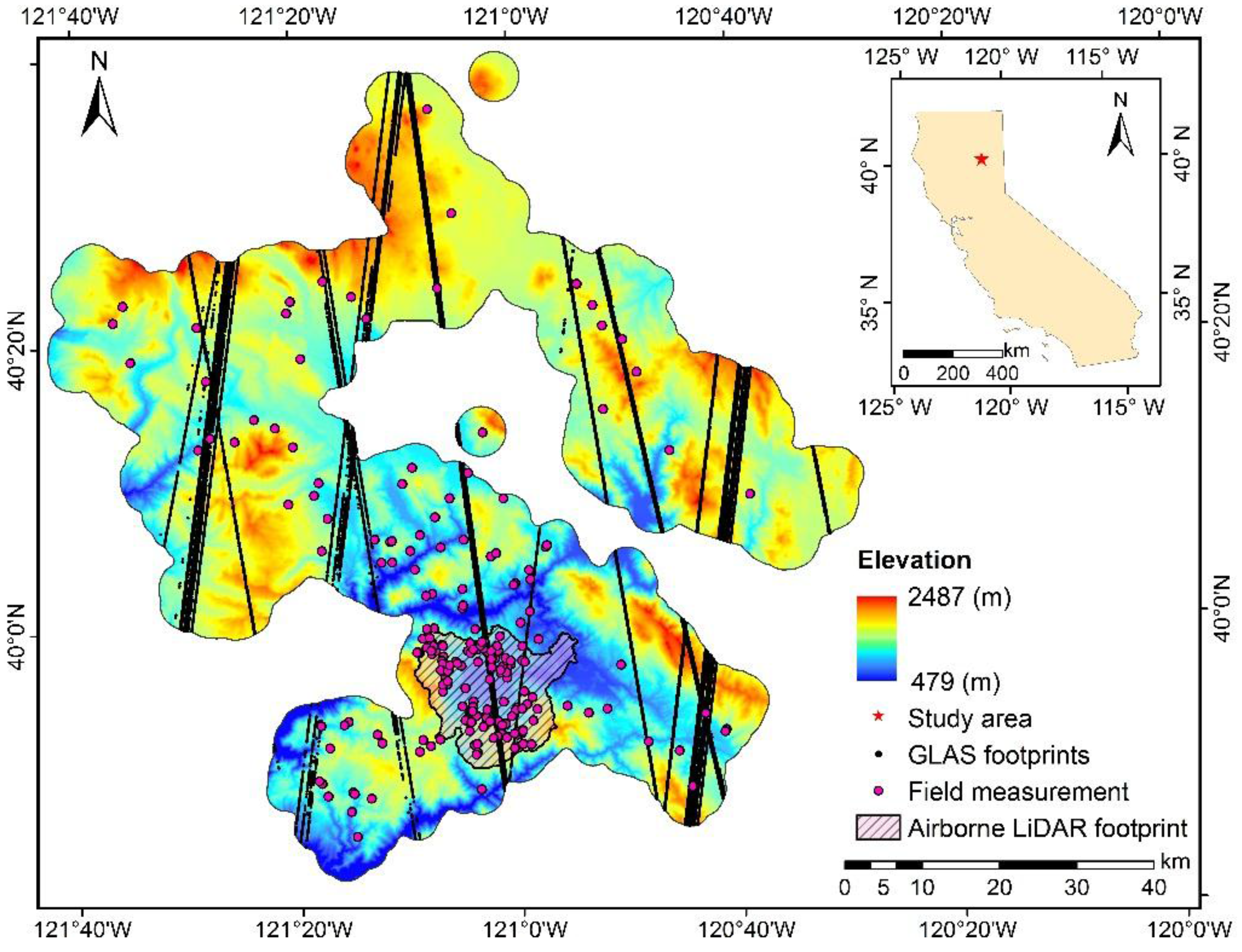
The study site is within the Plumas and Lassen National Forest, located in the northern Sierra Nevada, California, U.S. (Figure 1). It covers an area of 5022 km2. Its elevation ranges from 479 m to over 2500 m, and the average elevation is 1640 m. The slope of the study site can reach to 73°, and the average slope is 13°. The study site is dominated by mixed conifer forest, including incense cedar (libocedrus decurrens), lodgepole pine (pinus contorta), sugar pine (pinus lambertiana), ponderosa pine (pinus ponderosa), jeffrey pine (pinus jeffreyi), grey pine (pinus sabiniana), western juniper (juniperus occidentalis), Douglas-fir (pseudotsuga menziesii), California red fir (abies magnifica), and white fir (abies concolor). The major hardwoods within the mixed conifer stands are black oak (quercus kelloggii) and canyon live oak (quercus chrysolepis).

Figure 1.
The location of the study area, and the distribution of Geoscience Laser Altimeter System (GLAS) footprints, airborne light detection and ranging (LiDAR) data and in-situ measurements. Note that the elevation distribution in the figure is represented by the Shuttle Radar Topography Mission (SRTM) digital elevation model (DEM).
2.2. In-Situ Data
Within the study area, 239 plot measurements were obtained by the U.S. Forest Service based on the national forest inventory and analysis protocol [38]. These plots were originally set to study the behavior of California spotted owl (Strix occidentalis occidentalis), an endangered wildlife species in the Sierra Nevada. Each plot location was randomly selected and had to be potentially suitable for the owl to nest or forage. Within the airborne LiDAR footprint, plots were densified to generate and validate vegetation products from airborne LiDAR data. Each plot was composed of four sub-plots (956 in total), which were 14.62 m in diameter. In each sub-plot, tree height and diameter at the breast height (DBH) for each individual tree with a DBH lager than 12.7 cm were measured in the growing season between 2004 and 2009 using a laser range finder and diameter tape, respectively. Note that all computations and assessments in this study were performed at the sub-plot level. The elevation occupied by these subplots ranges from 940 m to 1950 m, and the mean elevation of all subplots is 1476 m; the slope ranges from near 0° to over 44°, and mean slope is 15°.
2.3. SRTM Data
The 11-day SRTM was a joint mission conducted by the NASA and NGA, which was flown in February 2000. It utilized a 225 km wide swath from an altitude of 233 km above the Earth. A radar interferometer operating in C-band (with a wavelength of 5.6 cm) was used to generate the globally consistent DEM products, covering approximately 99.97% of the Earth’s land surface from 56°S to 60°N. The 1 arc second (often quoted as 30 m) SRTM global DEM has been released in late 2014 and early 2015, and is available at the website of U.S. Geological Survey (USGS) [39]. The horizontal datum of the SRTM data is WGS84, and the vertical datum is the mean sea level determined by the WGS84 Earth gravitational model geoid. In this study, to keep in accordance with all other datasets, the horizontal coordinates of the collected SRTM DEM was projected to UTM Zone 10 projection based on the ellipsoid of NAD1983, and the vertical coordinates were projected to NAVD88. The terrain slope was calculated from the SRTM DEM using the ESRITM ArcGIS software. It should be noted that all slope data mentioned hereafter refer to the SRTM DEM-derived slope product.
2.4. Spaceborne LiDAR Data
GLAS onboard the NASA ICESat was a full-waveform LiDAR sensor, which was first launched in January 2003, and operated for seven years before being retired in February 2010. It was designed for measuring ice sheet elevations and changes in elevation through time, and obtaining global-scale cloud and aerosol height profiles, land elevation and vegetation cover, and sea ice thickness. However, these measurements were not spatially consistent. Its footprints had a nominal diameter of 65 m, and were spaced at 170 m along tracks and tens of kilometers across tracks.
In this study, we collected all available GLA01, GLA06 and GLA14 products from the ICESat/GLAS data pool [40]. The GLA01 product provided the full-waveform measurements, the GLA06 product provided the geolocation and data quality for each full-waveform record, and the GLA14 product provided the land surface elevation information of each footprint. These three products were linked together using the unique ID and shot time of each laser pulse. For GLAS footprints within the study area, four filtering criteria were used to ensure the quality of GLAS measurements: (1) should be obtained under cloud-free condition; (2) should have no saturation effect; (3) should have high signal to noise ratio; and (4) should not be significantly higher (i.e., 100 m) than the land surface elevation described by the SRTM DEM.
There were finally 13,716 GLAS full-waveform records left within the study site (Figure 1). For each GLAS record, four parameters were extracted from the GLAS products, including land surface elevation, waveform extent, leading edge extent, and trailing edge extent. The land surface elevation was directly obtained from the GLA14 product. The waveform extent, leading edge extent and trailing edge extent were computed from the full-waveform information. These three parameters have been proved to be highly correlated to canopy height, canopy height variability and terrain slope [33,41,42,43,44]. Definitions of these three parameters can be found in Lefsky et al. (2007) [42], and will not be discussed in detail here. Note that the vertical datum of GLAS data is TOPEX/Poseidon, which is normally 71 cm higher than the commonly used WGS84 ellipsoid. In this study, all GLAS elevations were first subtracted by 71 cm, and then projected to NAVD88 using GEOID12B from National Geodetic Survey.
2.5. Airborne LiDAR Data
The airborne LiDAR data was collected at the bottom left of the study site (Figure 1); it covered about 5% (256.57 km2) of the total study area. The data was acquired between July and August 2009, using a Leica ALS50 II laser system mounted on a Cessna Caravan airplane. The LiDAR sensor allowed up to four range measurements per laser pulse, and the sensor scan angle was ±14° from nadir. To reduce the laser shadowing and increase LiDAR point density, each flight line was surveyed with an opposing flight line with a side-lap of ≥50%. The obtained LiDAR point cloud density ranged from 4.0–10.2 pt/m2 with a mean of 5.7 pt/m2. Ground control points, which were surveyed using a real-time kinematic GPS, were set to evaluate the positioning accuracy of the LiDAR data. The obtained horizontal and vertical accuracy of the LiDAR data were 31 cm and 3.5 cm, respectively.
Canopy quantile metrics, DEM, and canopy cover products for the airborne LiDAR footprint were directly computed from the airborne LiDAR data. Canopy quantile metrics, representing the height below X% of the LiDAR point cloud, are frequently used LiDAR products to estimate forest parameters that cannot be obtained directly from LiDAR point cloud [45,46]. In this study, 11 quantile metrics, i.e. 0%, 1%, 5%, 10%, 25%, 50%, 75%, 90%, 95%, 99%, and 100%, were computed from the LiDAR point cloud at a resolution of 30 m. The DEM (at 30 m resolution) within the airborne LiDAR footprint was interpolated from the LiDAR ground returns using ordinary kriging, which has been proved to be more accurate than other interpolation schemes (e.g., inverse distance weighted and spline) for interpolating DEM from LiDAR-derived elevation points [21,23,47]. The canopy cover (at 30 m resolution) was computed using a canopy height model based method, which has been proven reliable and consistent for estimating canopy cover from LiDAR data [48].
2.6. Aerial Imagery
The National Agriculture Imagery Program (NAIP) aerial imagery taken in 2009 was used to generate the canopy cover product in the study area. The NAIP imagery is at 1 m resolution, and composed by blue band, green band, red band and near-infrared (NIR) band. The NAIP program is run by the Farm Service of U.S. Department of Agriculture for the purpose of making high-resolution digital orthographies available to maintain common land units. All NAIP images were taken under permitted weather conditions, and followed the specification of no more than 10% cloud cover per quarter quad tile. The Aerial Photography Field Office (APFO) has adjusted and balanced the dynamic range of each image tile to full range of Digital Number (DN) value (0–255), and orthorectified each image file using National Elevation Dataset before releasing the data [49].
2.7. Landsat TM Imagery
The Landsat 5 TM data were collected from the USGS website for the study site during the growing season of 2009 [50]. In total, nine scenes of surface reflectance data, generated using 6S (Second Simulation of a Satellite Signal in the Solar Spectrum) radiative transfer models [51], were downloaded for the tree height mapping procedure. Visual examination was performed on each scene to ensure that there was less than 5% cloud or snow coverage in the image. The cumulative normalized difference vegetation index (NDVI) and maximum value composite (MVC) were calculated from the time-series TM imagery. The use of cumulative NDVI can increase the estimation accuracy of forest parameters compared with the use of NDVI data from a single time period [52]. MVC imagery has been demonstrated to be highly related to green-vegetation dynamics [53], and is capable of minimizing the problems common to single-date optical imagery, such as cloud contamination, atmospheric attenuation, surface directional reflectance, and view and illumination geometry [53].
2.8. Climate Surfaces
Four climate surfaces, namely annual mean temperature, annual temperature seasonality, annual total precipitation, and annual precipitation seasonality between 1950 and 2000 were calculated within the study area at 30 m resolution. The monthly mean temperature and monthly total precipitation across the western U.S. created by Alvarez et al. (2014) [37] were used to generate these four climate surfaces. For each year, the mean temperature and total precipitation were directly calculated from the monthly layers, and the temperature seasonality and precipitation seasonality were computed from the following equation:
where Seasonality represents the temperature seasonality or precipitation seasonality of the corresponding year, and SDmonthly and Meanmonthly are the standard deviation and mean of the monthly mean temperature (in Kelvin) or monthly total precipitation (in millimeter) for the corresponding year. The annual mean temperature, annual temperature seasonality, annual total precipitation, and annual precipitation seasonality were derived from the averages of corresponding yearly products.
3. Methodology
Generally, the procedure of the SRTM DEM correction method can be divided into three modules (Figure 2): (1) develop methods to estimate vegetation products (i.e., canopy cover and tree height) from multi-source datasets; (2) build the SRTM DEM correction model within the airborne LiDAR footprint; (3) estimate the SRTM DEM error and therefore correct the SRTM DEM across the study site. The detailed procedures and methods to estimate vegetation parameters and correct the SRTM DEM will be described in the following sections.
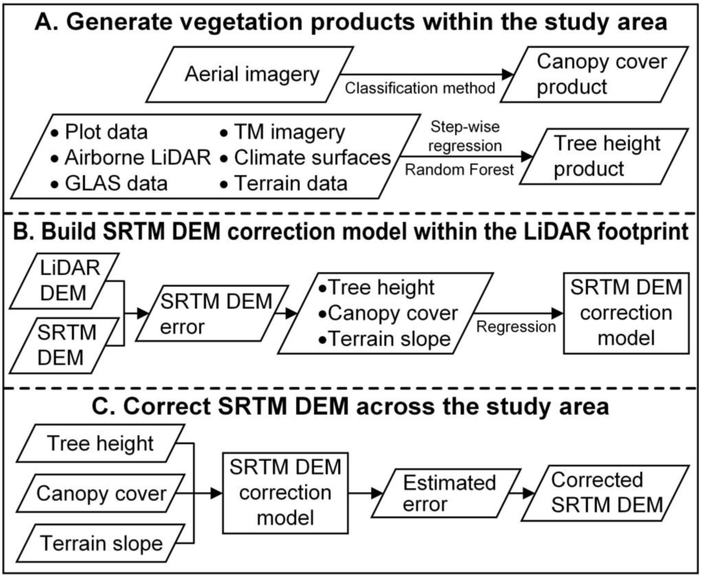
Figure 2.
Flow chart of the method to correct the SRTM DEM over vegetated mountain areas in this study.
Figure 2.
Flow chart of the method to correct the SRTM DEM over vegetated mountain areas in this study.

3.1. Canopy Cover Estimation Procedure
The canopy cover for the whole study site was calculated from aerial imagery using a classification method. The NAIP imagery was classified into two land cover types, tree and non-tree, using the Support Vector Machine algorithm. The training samples were randomly selected, and the attribute (tree/non-tree) of each sample was determined by visual examination. Considering the similarities in the spectral reflectance characteristics of forest canopies and grass [54], we further extracted seven texture layers (including mean, variance, homogeneity, contrast, dissimilarity, entropy and second moment) from each spectral band using the gray-level co-occurrence matrix (GLCM) filtering method, and included them in the classification procedure. Because grasslands usually have a smoother texture than trees, the use of these texture parameters was expected to reduce the chance of misclassification between trees and grass [55,56]. Procedures on how to calculate the GLCM matrix and extract texture parameters from the GLCM matrix can be found in Haralick et al. (1973) [57], and will not be discussed in detail here. The accuracy of the classification result was evaluated by independent and randomly-selected samples that were different from training samples. Finally, to calculate the canopy cover, the classification result in 1 m resolution was overlaid with a 30 m grid. The canopy cover for each 30 m × 30 m cell was calculated as the percentage of tree pixels within each corresponding cell. Since there was no field observed canopy cover, the estimated canopy cover product was evaluated by the airborne LiDAR-derived canopy cover, considering the strong capability of airborne LiDAR in estimating canopy forest structures [48,58].
3.2. Tree Height Estimation Method
In this study, the tree height distribution across the whole study site was calculated through the combination of multi-source datasets. It should be noted that the tree height mentioned hereafter refers to the Lorey’s height. For the field measurements, the Lorey’s height at the sub-plot scale (HL) was calculated from individual tree height (h) and basal area (b) using the following equation,
where i is the ith tree within a sub-plot, and n is the total number of trees in a sub-plot.
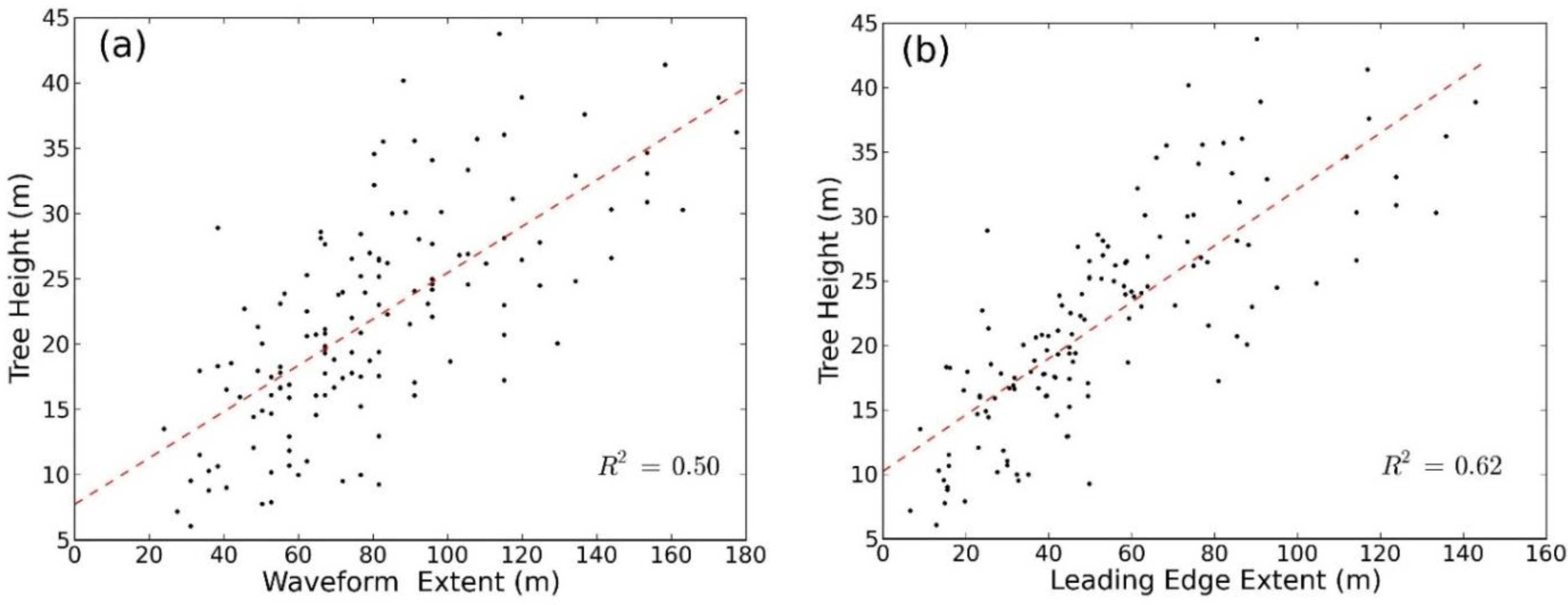
Figure 3 shows the procedure to estimate tree height from multi-source datasets. Within the airborne LiDAR footprint, we firstly estimated the tree height distribution from canopy quantile metrics using the step-wise regression method. Then, this airborne LiDAR derived tree height product was used to spatially link with GLAS parameters in the airborne LiDAR footprint, and therefore build a regression model between the airborne LiDAR-derived tree height and GLAS parameters. Lefsky et al. (2007) [42] found that GLAS waveform extent and leading edge extent were linearly correlated with the airborne LiDAR-derived tree height. As can be seen in Figure 4, the R2 for correlations between tree height and waveform extent and between tree height and leading edge extent were both higher than 0.5. Moreover, GLAS parameters, especially waveform extent and trailing edge extent, were influenced by terrain relief [42]. Therefore, the multiple linear regression method was used to build the correlation among airborne LiDAR-derived tree height, GLAS parameters and slope [41,42]. This regression model was applied to estimate tree heights for all GLAS footprints within the whole study site.
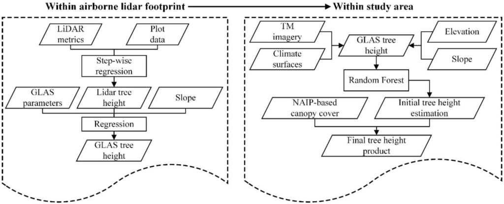
Figure 3.
The procedure of estimating forest tree height in the study area through the combination of multi-source datasets.
Figure 3.
The procedure of estimating forest tree height in the study area through the combination of multi-source datasets.

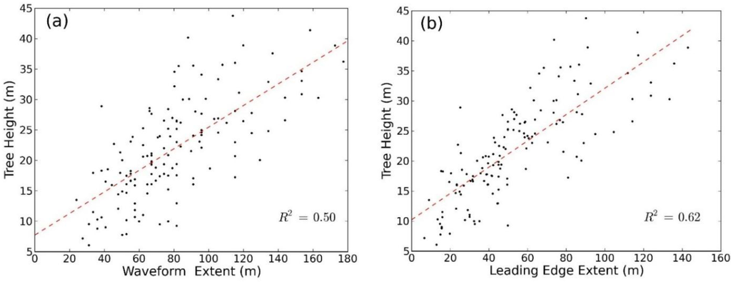
Figure 4.
(a) Correlation between airborne LiDAR-derived tree height and GLAS waveform extent; (b) Correlation between airborne LiDAR-derived tree height and GLAS leading edge extent. R2 represents the coefficient of determination. The red dashed lines are fitted lines between airborne LiDAR-derived tree height and GLAS parameters.
The obtained GLAS tree heights were used as a training dataset to extrapolate the tree height estimations to the whole study site. In this study, the regression tree method Random Forest (RF) [59] was used to estimate the tree height distribution from 13 predictors, i.e., six Landsat TM MVC bands (excluding the thermal band), cumulative NDVI, four climate surfaces, elevation, and slope. The RF algorithm was selected because there have been studies showing that it outperformed other parametric regression methods in estimating forest structures from GLAS parameters [31,36,43]. The RF extrapolation method was implemented using the randomForest R package [60], which included both classification and regression functions. We used manual iterative examination method to determine the optimized parameters to construct the “forest”, i.e., number of trees and number of variables tried at each split [60]. The number of trees and number of variables tried at each split were increased by one iteratively, and the values that produced the minimum mean-squared error were selected to extrapolate the GLAS tree height measurements. Here, based on manual iterative examination, 500 “RF trees” were included and four variables were tried at each split. The significance of variables used in the extrapolation process was evaluated by the percentage increase in the mean-squared error (%IncMSE) and the increase in node purity (IncNodePurity) [60]. Finally, the canopy cover data obtained from Section 3.1 was used to mask the initial tree height estimation. Tree heights at areas without tree coverage (canopy cover equaled to zero) were assigned as zero meter in the final tree height product. The estimated tree height product across the whole study area was assessed by field plot measurements.
3.3. SRTM DEM Correction Method
Su & Guo et al. (2014) [30] found that a multiple linear regression model of the SRTM DEM error depending on vegetation parameters and terrain slope can be used to correct the SRTM DEM efficiently. However, their regression model was developed based on airborne LiDAR-derived vegetation parameters, and could not be applied to areas without airborne LiDAR coverage. In this study, we developed a similar regression method to correct the SRTM DEM based on above-mentioned vegetation products obtained from multi-source datasets.
Firstly, we evaluated the SRTM DEM accuracy using the LiDAR DEM. For each SRTM DEM pixel within the airborne LiDAR coverage, we calculated differences between the SRTM DEM and the LiDAR DEM. Then, two-thirds of these pixels were randomly selected to build the SRTM DEM calibration model. A multiple linear regression model of the SRTM DEM error depending on the estimated canopy cover and tree height products and terrain slope derived from the SRTM DEM was developed based on these randomly selected training pixels. Finally, this regression model was applied to the whole study site to estimate the SRTM DEM error from the estimated canopy cover, tree height, and terrain slope and therefore calibrate the SRTM DEM. The accuracy of the corrected SRTM DEM was assessed by the remaining one-third LiDAR DEM pixels and GLAS elevations.
3.4. Accuracy Assessment
The accuracy of the estimated canopy cover and tree height products and the corrected SRTM DEM was evaluated using coefficient of determination (R2) and root-mean-squared error (RMSE), which can be computed by the following equations,
where n is the number of samples, xi is the ith original value, i is the ith modeled value, and is the mean of all original values. Besides, the test statistic was taken for all coefficients and constants obtained from multiple linear regression analysis at the significance level (α) of 0.05 or 0.01. The null hypothesis for the test statistic was that the obtained coefficients and constants should be zero. If the probability of obtaining this null hypothesis (known as p-value, denoted as p) was smaller than the significance level, the null hypothesis was rejected and the obtained coefficients were recognized as statistically significant.
4. Results
4.1. Canopy Cover Estimation
Figure 5a shows the estimated canopy cover distribution in the study area. The average canopy cover in the study area is 53% and the standard deviation is 26%. The canopy cover is generally higher in the eastern part of the study site than in the western part. Moreover, as can be seen in Figure 5a, there is a “banding” effect associated with the aerial imagery flight lines. The airborne LiDAR-derived canopy cover was used to evaluate the accuracy of the estimated canopy cover product. The R2 between the estimated canopy cover and airborne LiDAR-derived canopy cover is as high as 0.71, and the mean absolute difference is about 12%. The mean and standard deviation of the canopy cover from airborne LiDAR data is 60.9% and 27.0%, which are 2% lower and 4% higher than those from the estimated canopy cover product, respectively. As can be seen in Figure 5b, the estimated canopy cover is slightly higher than the LiDAR-derived canopy cover in all canopy cover groups. Both the mean and median of differences between the estimated canopy cover and the airborne LiDAR-derived canopy cover are closer to zero with the increase of canopy cover, and the range of differences decreases with the increase of the canopy cover.
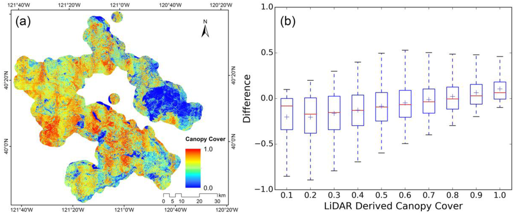
Figure 5.
(a) Estimated canopy cover distribution from aerial imagery in the study area; (b) Boxplot of differences between the airborne LiDAR-derived canopy cover and the estimated canopy cover within the airborne LiDAR footprint (airborne LiDAR-derived canopy cover minus estimated canopy cover). The blue “+” indicates the mean difference of the corresponding group. Numbers 0.1–1.0 on x axis represent the airborne LiDAR-derived canopy cover group of 0–0.1, 0.1–0.2, 0.2–0.3, 0.3–0.4, 0.4–0.5, 0.5–0.6, 0.6–0.7, 0.7–0.8, 0.8–0.9, and 0.9–1.0, respectively.

4.2. Tree Height Estimation
In this study, four LiDAR canopy quantile metrics, including 25%, 50%, 75% and 100%, were selected by the step-wise regression model to calculate tree height from airborne LiDAR data. The R2 between these four canopy quantile metrics and field observations is 0.70. This airborne LiDAR-derived tree height was linked with GLAS parameters, and a multiple linear regression model was developed to calculate tree height from GLAS parameters,
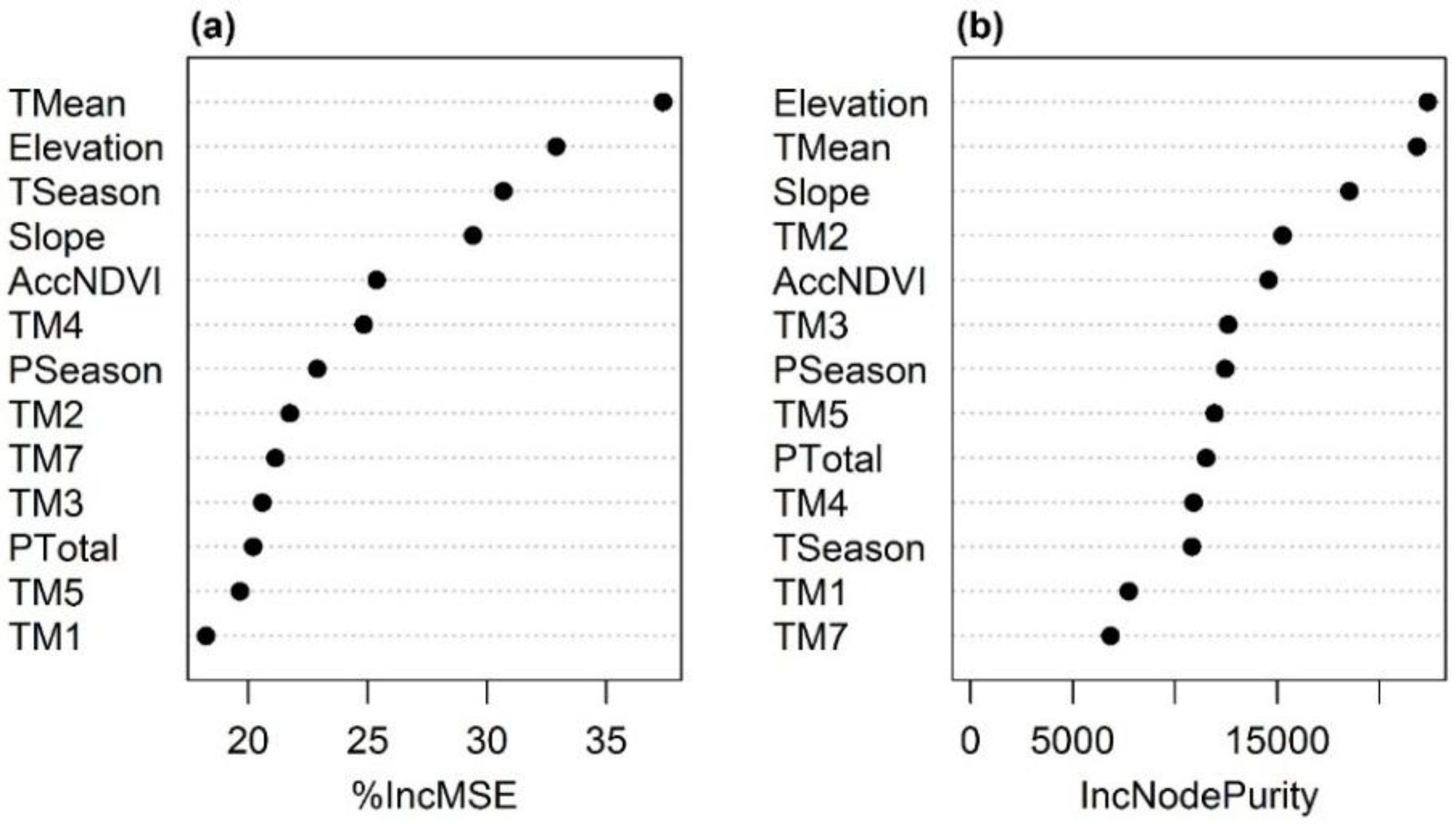
where THGLAS represents the GLAS-derived tree height, WE represents the waveform extent, LE represents the leading edge extent, TE represents the trailing edge extent, and S represents the terrain slope. This equation was applied to all GLAS footprints within the study area to calculate tree height at the GLAS footprints. Finally, a RF regression model was built to extrapolate the tree height estimations from GLAS footprints to the whole study area. The RF regression model built from the selected multi-source datasets can explain 72% of the variances in tree height. Figure 6 shows the importance of variables in the built RF regression model. As can be seen, regardless of whether the evaluation was performed using %IncMSE or IncNodePuri, the absence of annual mean temperature, elevation, annual temperature seasonality, slope and cumulative NDVI significantly increased the mean-squared error and node purity, indicating a decrease in the prediction accuracy of the built RF regression tree model.
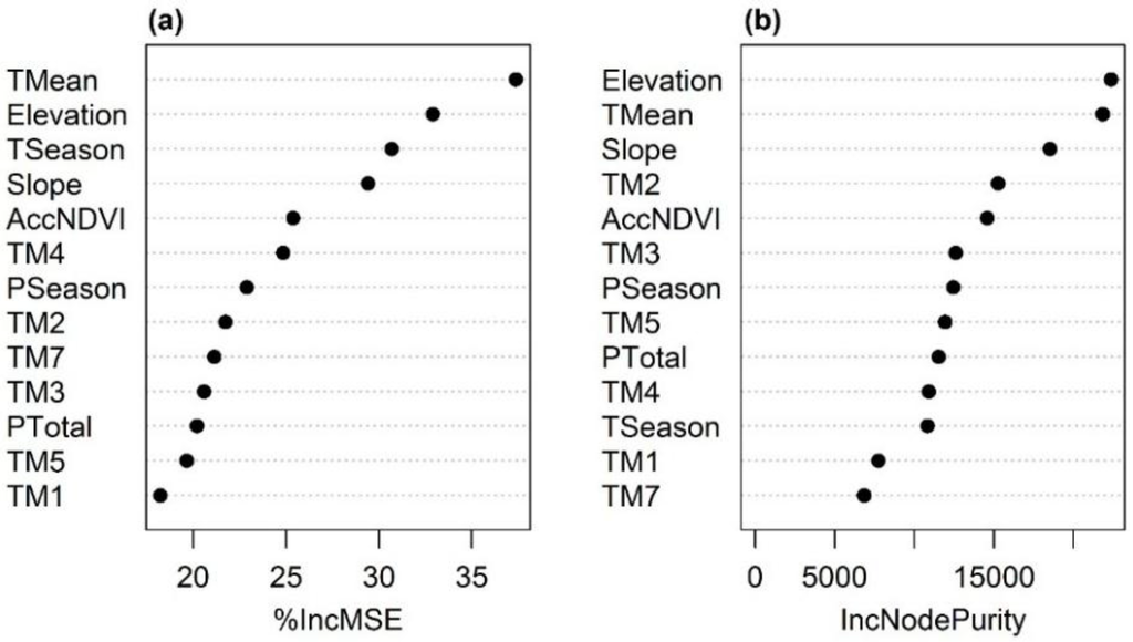
Figure 6.
Variable importance for the tree height estimation Radom Forest model, denoted by (a) the percentage increase of mean-squared error (%IncMSE) and (b) the increase in node purity (IncNodePurity). PTotal, PSeason, TMean, TSeason, AccNDVI, and TM 1–5 and 7 represent the annual total precipitation, annual precipitation seasonality, annual mean temperature, annual temperature seasonality, cumulative NDVI, and six TM spectral bands, respectively.
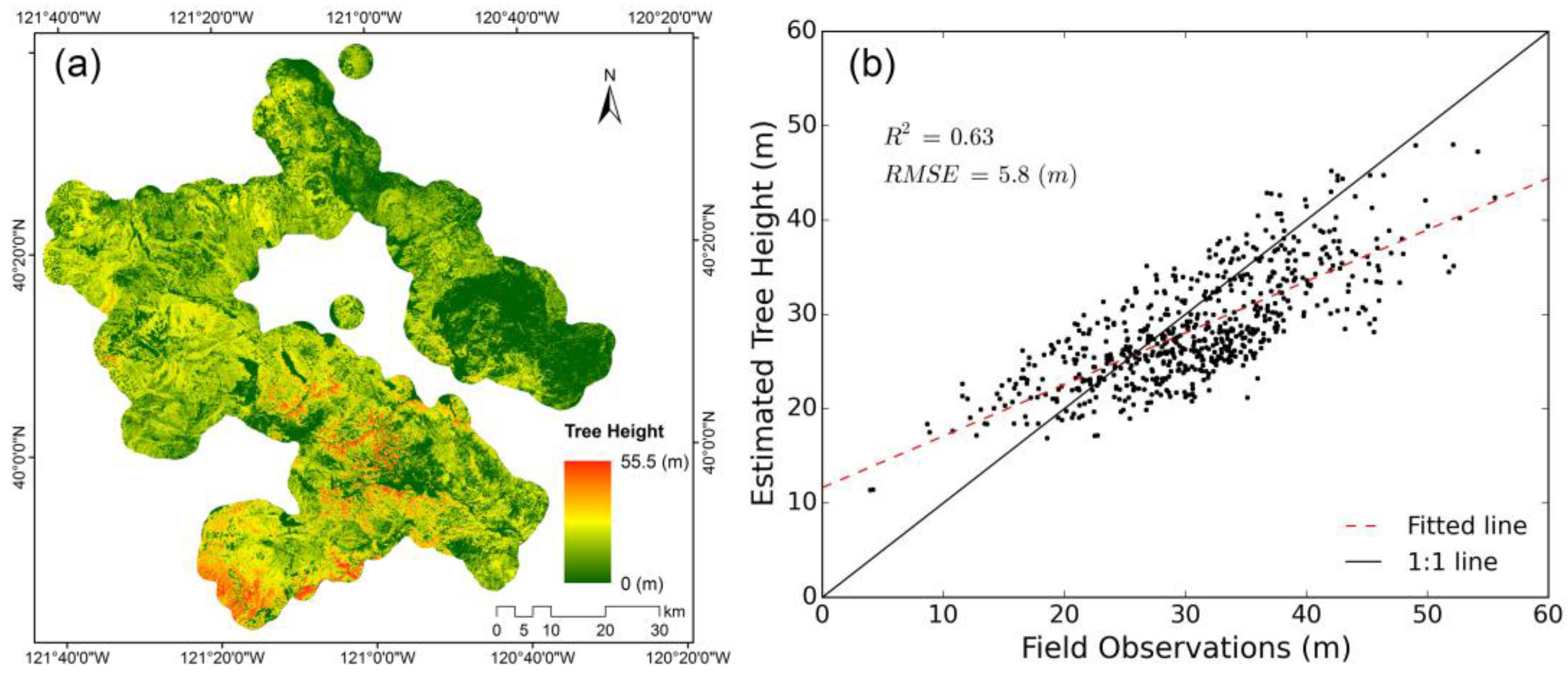
The estimated tree height distribution is shown in Figure 7a. As can be seen, the tree height is generally higher in the southern part of the study site than in the northern part. It ranges from 0–55.5 m, with a mean of 18.3 m and a standard deviation of 11.8 m. The field plot measurements were used to evaluate the accuracy of the tree height estimation. As shown in Figure 7b, the R2 between the estimated and field-measured tree height is 0.63, and the RMSE is 5.8 m. The fitted line between the predicted and field measured tree height is close to the 1:1 line. However, the proposed tree height estimation method still overestimated tree height with relatively low values (<15 m) and underestimated tree height with relatively high values (>40 m).

Figure 7.
(a) Estimated tree height distribution in the study area; (b) Scatter plot between the estimated tree height and field observations.
Figure 7.
(a) Estimated tree height distribution in the study area; (b) Scatter plot between the estimated tree height and field observations.
4.3. SRTM DEM Correction
The accuracy of the SRTM DEM was evaluated by comparing with the LiDAR DEM. As can be seen in Figure 8, the SRTM DEM is over 12 m higher than the LiDAR DEM on average, and the highest difference can reach to over 60 m. The standard deviation of differences between the SRTM DEM and the LiDAR DEM is around 11 m. Over 88% of the SRTM DEM pixels are higher than the LiDAR DEM. The systematic positive difference between the SRTM DEM and the LiDAR DEM further proves that the SRTM radar phase center can hardly reach the ground in vegetated mountain areas.
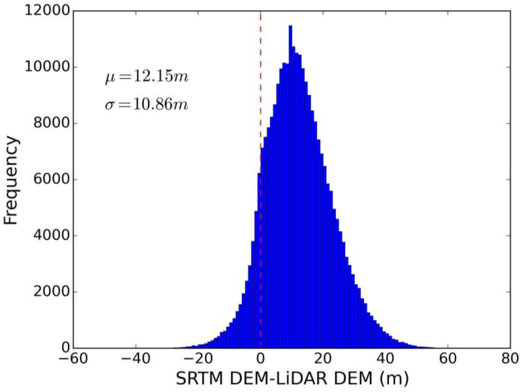
Figure 8.
Histogram of differences between the SRTM DEM and the LiDAR DEM (SRTM DEM minus LiDAR DEM). µ and σ represent the mean and standard deviation of differences between the SRTM DEM and the LiDAR DEM, respectively.
Figure 8.
Histogram of differences between the SRTM DEM and the LiDAR DEM (SRTM DEM minus LiDAR DEM). µ and σ represent the mean and standard deviation of differences between the SRTM DEM and the LiDAR DEM, respectively.

The distribution of the SRTM errors is highly correlated with vegetation and terrain conditions (Table 2). Specifically, the SRTM error increases rapidly with tree height. The mean difference between the SRTM DEM and the LiDAR DEM (SRTM DEM minus LiDAR DEM) for the group with trees higher than 40 m is almost eight times as large as that for the group with trees lower than 5 m. The standard deviation of differences also increases with the tree height, but not as significantly as the mean difference. Canopy cover has a similar effect on the SRTM error. The mean difference between the SRTM DEM and the LiDAR DEM for the group with canopy cover higher than 90% is over eight times larger than that for the group with canopy cover lower than 10%, and the standard deviation is about 3 m higher. Compared to the influence of tree height and canopy cover, slope has no significant influence on the mean difference between the SRTM DEM and the LiDAR DEM. However, it has more pronounced influence on the standard deviation of differences between the SRTM DEM and the LiDAR DEM. As can be seen in Table 2, the standard deviation has an over 15 m increase from the group with slope lower than 5° to the group with slope higher than 40°.
Table 2.
Statistics for differences between the SRTM DEM and the LiDAR DEM (SRTM DEM minus LiDAR DEM), classified by tree height, canopy cover and slope.
| Tree Height (m) | Canopy Cover (%) | Slope (°) | |||||||||
|---|---|---|---|---|---|---|---|---|---|---|---|
| Group | Mean a | STD b | N c | Group | Mean a | STD b | N c | Group | Mean a | STD b | N c |
| 0–5 | 3.04 | 7.39 | 34,387 | 0–10 | 2.11 | 7.68 | 15,482 | 0–5 | 9.52 | 8.07 | 43,494 |
| 5–10 | 6.01 | 8.17 | 13,952 | 10–25 | 4.57 | 9.06 | 15,438 | 5–10 | 12.12 | 8.43 | 69,034 |
| 10–20 | 7.91 | 8.71 | 40,121 | 25–50 | 7.21 | 8.89 | 44,492 | 10–20 | 12.72 | 10.66 | 111,021 |
| 20–30 | 13.33 | 9.95 | 139,790 | 50–75 | 11.76 | 9.58 | 87,439 | 20–30 | 13.12 | 14.35 | 41,927 |
| 30–40 | 20.67 | 10.30 | 42,986 | 75–90 | 15.15 | 10.19 | 65,838 | 30–40 | 12.80 | 18.20 | 7783 |
| ≥40 | 24.35 | 10.12 | 2751 | 90–100 | 19.29 | 10.86 | 45,298 | ≥40 | 13.30 | 23.13 | 724 |
a “Mean” represents the mean difference between the SRTM DEM and the LiDAR DEM; b “STD” represents the standard deviation of differences between theSRTM DEM and the LiDAR DEM; c “N” represents the the number of pixels in each group.
As mentioned in Section 3.3, two thirds of the LiDAR DEM were randomly selected to build the regression model of the SRTM DEM error dependent on tree height, canopy cover and slope. The built regression equation is described as follows,
where ε represents the SRTM DEM error, TH represents the tree height, CC represents the canopy cover, and S represents the terrain slope. The R2 for the built regression model is 0.52, and all coefficients in the model are statistically significant (p = 0.000 at α = 0.01). This model was then applied to the whole study area to compute the SRTM DEM errors, and therefore calibrate the SRTM DEM.
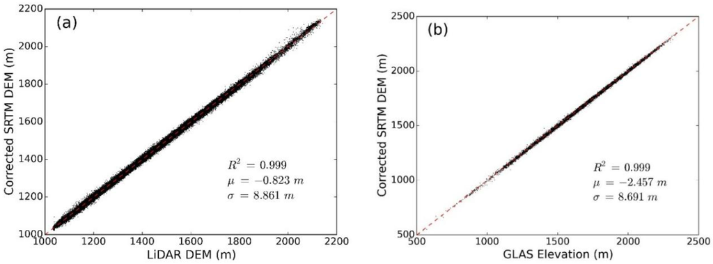
Figure 9.
(a) Scatter plot between the corrected SRTM DEM and the LiDAR DEM; (b) Scatter plot between the corrected SRTM DEM and GLAS elevations within GLAS footprints. R2 represents the coefficient of determination, and µ and σ represent the mean and standard deviation of differences between the corrected SRTM DEM and the LiDAR DEM (or GLAS elevations) (SRTM DEM minus LiDAR DEM or GLAS elevations). The red dashed line represents the 1:1 line.
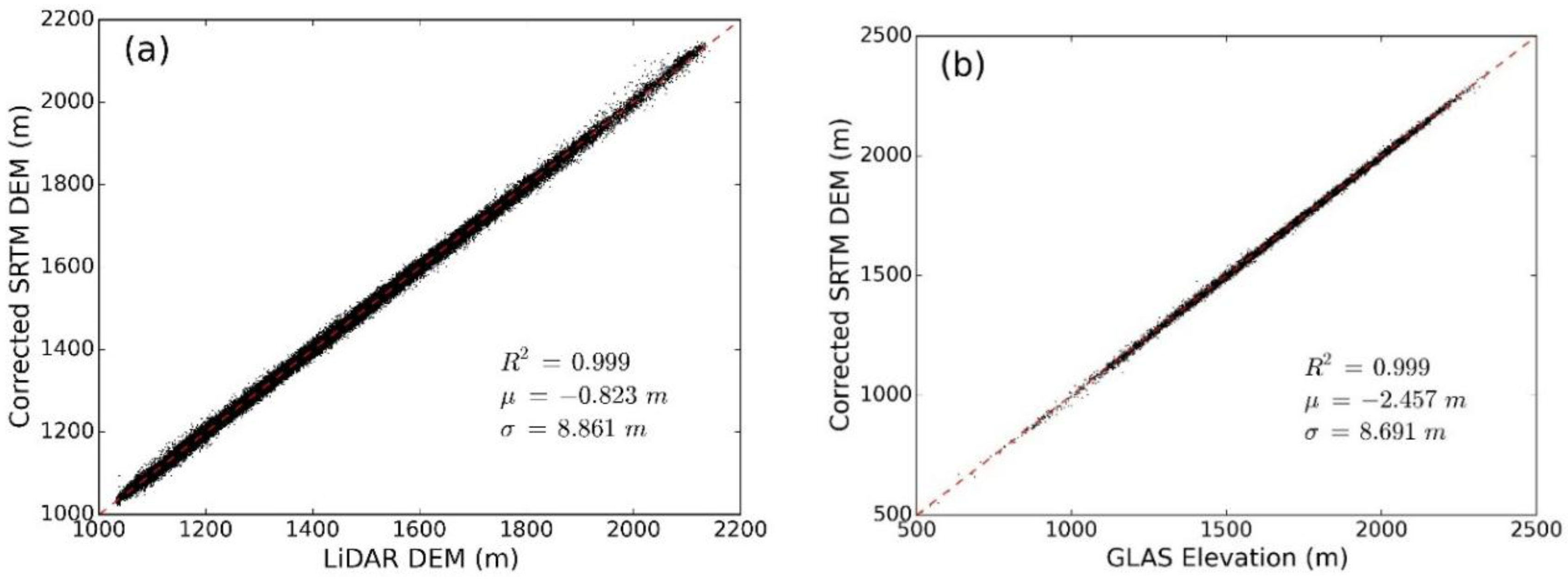
The corrected SRTM DEM was evaluated by the remaining one third of the LiDAR DEM pixels and GLAS elevations, respectively. As can be seen in Figure 9a, the corrected SRTM DEM shows a very good correspondence with the LiDAR DEM. The mean difference between the corrected SRTM DEM and the LiDAR DEM has decreased significantly, which is very close to 0 m. The standard deviation of differences between the corrected SRTM DEM and the LiDAR DEM also has a ~2 m drop, compared to the original SRTM DEM. The corrected SRTM DEM also shows a good correspondence with GLAS elevations (Figure 9b). However, the corrected SRTM DEM is about 2.5 m lower than the GLAS elevation on average. The standard deviation of differences between the corrected SRTM DEM and GLAS elevations is almost identical with that between the corrected SRTM DEM and the LiDAR DEM.
5. Discussions
5.1. Accuracy of Estimated Vegetation Parameters
In this study, canopy cover and tree height products were estimated to correct the SRTM DEM. The estimated canopy cover and tree height products showed good correspondences with either corresponding airborne LiDAR products or field measurements. However, systematic biases remain in the products. As can be seen in Figure 5b, the estimated canopy cover is systematically higher than the airborne LiDAR-derived canopy cover product, and the bias decreases with the increase of canopy cover. This result is consistent with previous studies [61,62], and may be caused by the misclassification of grass and low shrubs as trees in the aerial imagery classification procedure. At an individual pixel level, forest canopies, grass and low shrubs have very similar spectral reflectance characteristics [54]. Although the use of texture information can help to reduce the misclassification rate [55,56], it may not be used to totally remove grass and low shrubs from the tree group. The increased proportion of “tree” given by the misclassification of grass and low shrubs in areas with few trees tends to elevate canopy cover relative to that calculated from airborne LiDAR. With the increase of canopy cover, the possibility of misclassification may become smaller because grass and low shrubs are blocked by the forest canopy in aerial imagery, and therefore the estimated canopy cover is closer to the airborne LiDAR-derived canopy cover. Moreover, there is a noticeable “banding” effect in the estimated canopy cover product associated with flight lines (Figure 5a), which is possibly caused by the non-linear color-balancing problem of the NAIP imagery. The NAIP images were acquired at different time and under different weather conditions, which led the images from different flight lines to have dynamic ranges of DN values [49]. Although the APFO has adjusted and balanced the images into the same range (0–255) before releasing the data, the priority goal of the process was to make the images look “pleasant” instead of radiometrically correcting the images, because the NAIP imagery was primarily for public use. Using other high resolution imagery (e.g., QuickBird and WorldView) or performing a systematic radiometric correction on the NAIP imagery may be helpful to solve this “banding” effect.
As for tree height, the estimated product inclined to slightly overestimate the tree heights in areas with small trees and underestimate the tree heights in areas with big trees (Figure 7b). The overestimation of tree heights in areas with low vegetation may also be related to the existence of grass. In this study, we used spectral reflectance characteristics from Landsat TM as a data source to extrapolate tree height estimations from GLAS footprints to spatially continuous layers. Similar to aerial imagery, Landsat TM imagery also has similar spectral reflectance characteristics between grass and trees [63]. Although GLAS parameters can be used to estimate forest structures accurately within GLAS footprints, the similarity in the spectral reflectance between grass and trees may overestimate the height of grass during the extrapolation process, and therefore increase the overall tree height estimation in areas with low tree coverage. Moreover, because of the limited penetration capability in vegetated areas, estimating forest structure parameters from Landsat TM imagery usually suffered from saturation effect [64,65]. The use of other ancillary datasets, e.g. climate surfaces and topographic data, can help to reduce the saturation effect in the extrapolation process, but may not be used to totally eliminate its influence on the result. Additionally, the in-situ measurements are densified in the airborne LiDAR footprint (Figure 1), and this may lead to a biased accuracy assessment result because they are less representative of the whole region. To address this issue, we further evaluated the estimated tree height product only using the plot measurements outside of the airborne LiDAR footprint. The result shows that the obtained R2 and RMSE are 0.61 and 6.2 m, respectively, which are very close to those obtained from the accuracy assessment result using all plot measurements.
5.2. Comparisons among SRTM DEM, GLAS Elevations, LiDAR DEM and Corrected SRTM DEM
The SRTM DEM was found to be systematically higher than the actual land surface in vegetated mountain areas, which agrees with previous studies [26,27,28,30]. Different vegetation conditions and topographic conditions have a significant influence on the SRTM DEM error (Table 2). Specifically, the SRTM DEM error tends to be higher in areas with tall and dense forest. This may be caused by the absorption and reflection effects of forest canopy to the SRTM radar signal. The topographic conditions have more influence on the uncertainty of the SRTM DEM bias. As can be seen Table 2, the standard deviation of differences between the SRTM DEM and the LiDAR DEM increases rapidly with the slope. Su & Guo (2014) [30] argued that the influence of slope on the SRTM DEM error depends on other factors, i.e., terrain aspect, SRTM radar signal azimuth, and SRTM radar signal incidence angle. A rough terrain can either increase or decrease the distance needed for the SRTM radar signal to reach the ground based on different combinations of terrain aspect, SRTM radar signal azimuth and SRTM radar signal incidence angle. A larger slope can increase the variation of this distance and therefore increase the uncertainty of the SRTM DEM bias. Moreover, in this study, the slope product used to correct the SRTM DEM was derived from the SRTM DEM itself, and the SRTM DEM error might propagate to the slope product. However, the SRTM DEM error is a systematic bias in vegetated mountain areas, and may not significantly change the relative terrain relief. Therefore, the derived slope product may still reflect the terrain changes of adjacent areas. As mentioned, the terrain slope can influence the variability of the SRTM DEM bias. By including the SRTM DEM-derived slope into the correction procedure, the standard deviation of differences between the corrected SRTM DEM and the LiDAR DEM dropped by two meters approximately, which further indicates that the SRTM DEM-derived slope may be a valid parameter to correct the SRTM DEM.
Outside the airborne LiDAR footprint, the corrected SRTM DEM was evaluated based on the GLAS elevations. As can be seen in Figure 9b, the corrected SRTM DEM was found to be around 2.5 m lower than the GLAS elevations. This may be caused by the fact that the GLAS elevations overestimated ground elevations in vegetated areas [66]. In this study, we further compared the GLAS elevations with the LiDAR-derived DEM and the original SRTM DEM within the airborne LiDAR footprint. As shown in Figure 10, GLAS elevations are about 6 m higher than the LiDAR DEM and about 8 m lower than the SRTM DEM. Although the accuracy of the GLAS elevations is higher than the SRTM DEM, they are still systematically higher than the actual ground. The GLAS elevation error is also influenced by the vegetation conditions. Unlike the SRTM DEM error, GLAS elevation errors are not linearly influenced by the vegetation conditions. As can be seen in Table 3, in groups with tree height lower than 20 m or canopy cover lower than 50%, the mean biases of GLAS elevations are almost identical, which are around 3.5 m higher than the LiDAR DEM. However, in groups with tree height higher than 20 m or canopy cover higher than 50%, the mean biases of GLAS elevations increase significantly. This indicates that the GLAS laser pulse may still reach the land surface unless the forest density or forest height reach to a certain level. Moreover, the terrain slope has no significant influence on the mean difference of GLAS elevation errors. As shown in Table 3, the mean difference between GLAS elevations and the LiDAR DEM stays stable among different slope groups, except the group with slope higher than 30°. The large GLAS elevation bias for the group with slope higher than 30° may be caused by a relatively smaller number of samples. Besides, neither vegetation condition nor terrain slope has a significant influence on the standard deviation of GLAS elevation errors, which stays around 4–5 m for all groups (Table 3).

Figure 10.
(a) Histogram of differences between GLAS elevations and the LiDAR DEM (LiDAR DEM minus GLAS elevations); (b) Histograms of differences between GLAS elevations and the SRTM DEM (SRTM DEM minus GLAS elevations). µ and σ represent the mean and standard deviation of differences between GLAS elevations and the LiDAR DEM (or the SRTM DEM).
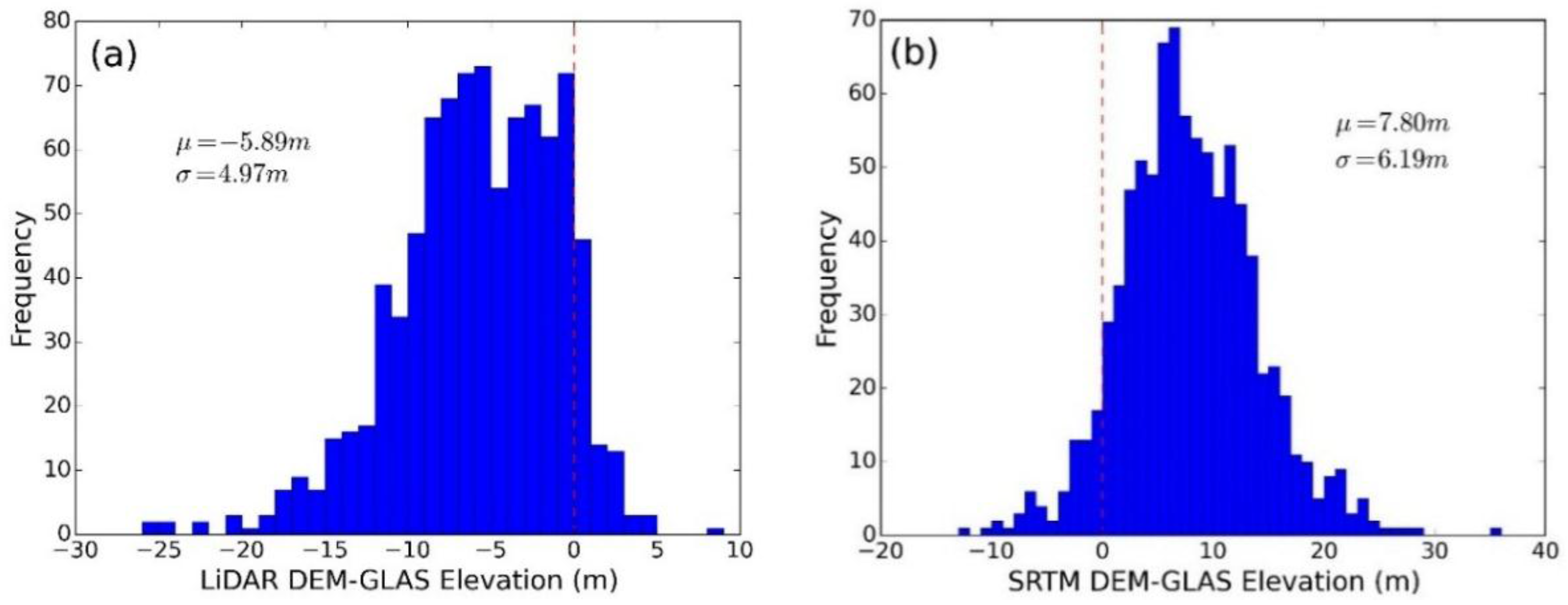
Table 3.
Statistics for differences between GLAS elevations and the LiDAR DEM (GLAS elevations minus LiDAR DEM), classified by tree height, canopy cover, and slope.
| Tree Height (m) | Canopy Cover (%) | Slope (°) | |||||||||
|---|---|---|---|---|---|---|---|---|---|---|---|
| Group | Mean a | STD b | N c | Group | Mean a | STD b | N c | Group | Mean a | STD b | N c |
| 0–5 | −3.49 | 3.92 | 74 | 0–10 | −3.58 | 4.85 | 36 | 0–5 | −5.45 | 5.25 | 120 |
| 5–10 | −3.68 | 3.93 | 35 | 10–25 | −1.10 | 2.75 | 50 | 5–10 | −5.57 | 4.77 | 284 |
| 10–20 | −3.62 | 4.24 | 172 | 25–50 | −3.54 | 4.25 | 201 | 10–20 | −6.23 | 5.02 | 420 |
| 20–30 | −6.38 | 4.89 | 469 | 50–75 | −6.47 | 4.58 | 423 | 20–30 | −5.57 | 4.98 | 56 |
| ≥30 | −9.04 | 4.79 | 133 | ≥75 | −9.08 | 4.71 | 173 | ≥30 | −9.02 | 6.62 | 3 |
a “Mean” represents the mean difference between GLAS elevations and the LiDAR DEM; b “STD” represents the standard deviation of differences between GLAS elevations and the LiDAR DEM; c “N” represents the the number of pixels in each group.
The SRTM DEM correction procedure shows great potential to correct the SRTM DEM in large spatial coverage. The mean difference between the corrected SRTM DEM and the LiDAR DEM is very close to zero (Figure 9a), indicating that the systematic bias of the SRTM DEM can be removed by the proposed method. By collecting more field observations and airborne LiDAR measurements covering different forest types, the proposed method in this study may even have the possibility to provide an improved version of the SRTM DEM in global scale. Hansen et al. (2013) [67] provided a global scale high-resolution forest cover product using the Earth observation satellite data. Simard et al. (2011) [36] and Lefsky (2010) [33] showed the possibility to estimate tree height distribution in global scale through the combination of MODIS data and GLAS data. Considering the availability of GLAS data, Landsat TM imagery and other ancillary datasets in global scale, it is possible to produce a global-scale tree height map in fine resolution. Moreover, Su & Guo et al. (2014) [30] demonstrated that a SRTM correction model based on one forest type is also applicable to areas with similar forest type coverage. Therefore, if we can gather airborne LiDAR data to cover more forest types, individual SRTM correction models can be developed for each forest type and therefore an improved global-scale SRTM DEM product may be achieved.
6. Conclusions
The SRTM DEM is systematically higher than actual land surface in vegetated mountain areas. The error of the SRTM DEM is significantly influenced by different vegetation and terrain conditions. In general, the SRTM DEM bias tends to be bigger in areas with high canopy cover and tall trees, and the uncertainty of SRTM DEM bias tends to be bigger in areas with steep slope. To correct the SRTM DEM in areas without airborne LiDAR coverage, this study first developed methods to estimate canopy cover and tree height from aerial imagery and multi-source datasets, respectively. The estimated canopy cover and tree height products show good correspondences with airborne LiDAR-derived canopy cover and field measurements, respectively. The R2 between the estimated canopy cover and the airborne LiDAR-derived canopy cover is 0.71, and that between the estimated tree height and field observations is 0.63. These obtained vegetation products were used along with the LiDAR DEM and slope derived from the SRTM DEM to build a SRTM DEM correction model. This model significantly improves the accuracy of the SRTM DEM. The mean difference between the corrected SRTM DEM and the LiDAR DEM decreases from over 12 m to −0.8 m, and the standard deviation drops from 10.86 m to 8.86 m. Besides, this study also examined the accuracy of GLAS elevations within the airborne LiDAR footprint. The GLAS elevations are more than 5 m higher than the LiDAR DEM on average. The corrected SRTM DEM is about 2.5 m lower than GLAS elevations across the whole study site, which further demonstrates that the proposed correction model can reduce the systematic bias of the SRTM DEM.
Acknowledgments
This study is supported by the National Science Foundation of China (project numbers 41471363 and 31270563). We thank the USGS and NASA for providing the SRTM DEM products. Thanks to John Keane and Ross Gerrard for giving constructive comments on generating the vegetation products. Thanks to Otto Alvarez for providing the climate surface products.
Author Contributions
Yanjun Su and Qinghua Guo conceived and designed the experiments; Yanjun Su and Qin Ma performed the experiments; Yanjun Su analyzed the data; Yanjun Su contributed materials and analysis tools; Yanjun Su, Qinghua Guo and Wenkai Li wrote the paper.
Conflicts of Interest
The authors declare no conflict of interest.
References
- Zhang, W.; Montgomery, D.R. Digital elevation model grid size, landscape representation. Water Resour. Res. 1994. [Google Scholar] [CrossRef]
- Franklin, S.; Peddle, D.; Dechka, J.; Stenhouse, G. Evidential reasoning with Landsat TM, DEM and GIS data for landcover classification in support of grizzly bear habitat mapping. Int. J. Remote Sens. 2002, 23, 4633–4652. [Google Scholar] [CrossRef]
- Falorni, G.; Teles, V.; Vivoni, E.R.; Bras, R.L.; Amaratunga, K.S. Analysis and characterization of the vertical accuracy of digital elevation models from the shuttle radar topography mission. J. Geophys. Res. 2005. [Google Scholar] [CrossRef]
- Koch, A.; Lohmann, P. Quality Assessment and Validation of Digital Surface Models Derived from the Shuttle Radar Topography Mission (SRTM). Available online: http://www.ipi.uni-hannover.de/uploads/tx_tkpublikationen/Paper620.pdf (accessed on 9 July 2015).
- Callow, J.N.; van Niel, K.P.; Boggs, G.S. How does modifying a DEM to reflect known hydrology affect subsequent terrain analysis? J. Hydrol. 2007, 332, 30–39. [Google Scholar] [CrossRef]
- Peters, D.L.; Prowse, T.D.; Pietroniro, A.; Leconte, R. Flood hydrology of the Peace-Athabasca Delta, northern Canada. Hydrol. Process. 2006, 20, 4073–4096. [Google Scholar] [CrossRef]
- Ludwig, R.; Schneider, P. Validation of digital elevation models from SRTM X-SAR for applications in hydrologic modeling. ISPRS J. Photogramm. Remote Sens. 2006, 60, 339–358. [Google Scholar] [CrossRef]
- Van Niel, K.P.; Laffan, S.W.; Lees, B.G. Effect of error in the DEM on environmental variables for predictive vegetation modelling. J. Veg. Sci. 2004, 15, 747–756. [Google Scholar] [CrossRef]
- Drake, J.M.; Randin, C.; Guisan, A. Modelling ecological niches with support vector machines. J. Appl. Ecol. 2006, 43, 424–432. [Google Scholar] [CrossRef]
- Kellndorfer, J.; Walker, W.; Pierce, L.; Dobson, C.; Fites, J.A.; Hunsaker, C.; Vona, J.; Clutter, M. Vegetation height estimation from shuttle radar topography mission and national elevation datasets. Remote Sens. Environ. 2004, 93, 339–358. [Google Scholar] [CrossRef]
- Franklin, S.E. Remote Sensing for Sustainable Forest Management; CRC Press: Boca Raton, FL, USA, 2001. [Google Scholar]
- Steelman, T.A.; Maguire, L.A. Understanding participant perspectives: Q-methodology in national forest management. J. Policy Anal. Manag. 1999, 18, 361–388. [Google Scholar] [CrossRef]
- Farr, T.G.; Kobrick, M. Shuttle radar topography mission produces a wealth of data. Eos Trans. Am. Geophys. Union 2000, 81, 583–585. [Google Scholar] [CrossRef]
- Rabus, B.; Eineder, M.; Roth, A.; Bamler, R. The shuttle radar topography mission—A new class of digital elevation models acquired by spaceborne radar. ISPRS J. Photogramm. Remote Sens. 2003, 57, 241–262. [Google Scholar] [CrossRef]
- Rodriguez, E.; Morris, C.S.; Belz, J.E. A global assessment of the SRTM performance. Photogramm. Eng. Remote Sens. 2006, 72, 249–260. [Google Scholar] [CrossRef]
- Bourgine, B.; Baghdadi, N. Assessment of C-band SRTM DEM in a dense equatorial forest zone. CR Geosci. 2005, 337, 1225–1234. [Google Scholar] [CrossRef]
- Berthier, E.; Arnaud, Y.; Vincent, C.; Remy, F. Biases of SRTM in high-mountain areas: Implications for the monitoring of glacier volume changes. Geophys. Res. Lett. 2006, 33, L08502. [Google Scholar] [CrossRef]
- Weydahl, D.J.; Sagstuen, J.; Dick, O.B.; Ronning, H. SRTM DEM accuracy assessment over vegetated areas in Norway. Int. J. Remote Sens. 2007, 28, 3513–3527. [Google Scholar] [CrossRef]
- Leon, J.; Cohen, T. An improved bathymetric model for the modern and palaeo Lake Eyre. Geomorphology 2012, 173, 69–79. [Google Scholar] [CrossRef]
- Farr, T.G.; Rosen, P.A.; Caro, E.; Crippen, R.; Duren, R.; Hensley, S.; Kobrick, M.; Paller, M.; Rodriguez, E.; Roth, L.; et al. The shuttle radar topography mission. Rev. Geophys. 2007. [Google Scholar] [CrossRef]
- Guo, Q.; Li, W.; Yu, H.; Alvarez, O. Effects of topographic variability and LiDAR sampling density on several DEM interpolation methods. Photogramm. Eng. Remote Sens. 2010, 76, 701–712. [Google Scholar] [CrossRef]
- Liu, X.Y.; Zhang, Z.Y.; Peterson, J.; Chandra, S. LiDAR-derived high quality ground control information and DEM for image orthorectification. Geoinformatica 2007, 11, 37–53. [Google Scholar] [CrossRef]
- Lloyd, C.D.; Atkinson, P.M. Deriving DSMs from LiDAR data with kriging. Int. J. Remote Sens. 2002, 23, 2519–2524. [Google Scholar] [CrossRef]
- Lohr, U. Digital elevation models by laser scanning. Photogramm. Rec. 1998, 16, 105–109. [Google Scholar] [CrossRef]
- Wehr, A.; Lohr, U. Airborne laser scanning—An introduction and overview. ISPRS J. Photogramm. Remote Sens. 1999, 54, 68–82. [Google Scholar] [CrossRef]
- Carabajal, C.C.; Harding, D.J. ICESat validation of SRTM C-band digital elevation models. Geophys. Res. Lett. 2005. [Google Scholar] [CrossRef]
- Carabajal, C.C.; Harding, D.J. SRTM C-band and ICESat laser altimetry elevation comparisons as a function of tree cover and relief. Photogramm. Eng. Remote Sens. 2006, 72, 287–298. [Google Scholar] [CrossRef]
- Bhang, K.J.; Schwartz, F.W.; Braun, A. Verification of the vertical error in C-band SRTM DEM using ICESat and Landsat-7, Otter Tail County, MN. IEEE Trans. Geosci. Remote Sens. 2007, 45, 36–44. [Google Scholar] [CrossRef]
- Hofton, M.; Dubayah, R.; Blair, J.B.; Rabine, D. Validation of SRTM elevations over vegetated and non-vegetated terrain using medium footprint LiDAR. Photogramm. Eng. Remote Sens. 2006, 72, 279–285. [Google Scholar] [CrossRef]
- Su, Y.; Guo, Q. A practical method for SRTM DEM correction over vegetated mountain areas. ISPRS J. Photogramm. Remote Sens. 2014, 87, 216–228. [Google Scholar] [CrossRef]
- Baccini, A.; Laporte, N.; Goetz, S.; Sun, M.; Dong, H. A first map of tropical Africa’s above-ground biomass derived from satellite imagery. Environ. Res. Lett. 2008. [Google Scholar] [CrossRef]
- Luckman, A.; Baker, J.; Kuplich, T.M.; Yanasse, C.D.C.F.; Frery, A.C. A study of the relationship between radar backscatter and regenerating tropical forest biomass for spaceborne SAR instruments. Remote Sens. Environ. 1997, 60, 1–13. [Google Scholar] [CrossRef]
- Lefsky, M.A. A global forest canopy height map from the Moderate Resolution Imaging Spectroradiometer and the Geoscience Laser Altimeter System. Geophys. Res. Lett. 2010. [Google Scholar] [CrossRef]
- Mitchard, E.; Saatchi, S.; White, L.; Abernethy, K.; Jeffery, K.; Lewis, S.; Collins, M.; Lefsky, M.; Leal, M.; Woodhouse, I.; et al. Mapping tropical forest biomass with radar and spaceborne LiDAR: Overcoming problems of high biomass and persistent cloud. Biogeosci. Discuss. 2011, 8, 8781–8815. [Google Scholar] [CrossRef]
- Saatchi, S.S.; Harris, N.L.; Brown, S.; Lefsky, M.; Mitchard, E.T.; Salas, W.; Zutta, B.R.; Buermann, W.; Lewis, S.L.; Hagen, S. Benchmark map of forest carbon stocks in tropical regions across three continents. Proc. Natl. Acad. Sci. USA 2011, 108, 9899–9904. [Google Scholar] [CrossRef] [PubMed]
- Simard, M.; Pinto, N.; Fisher, J.B.; Baccini, A. Mapping forest canopy height globally with spaceborne LiDAR. J. Geophys. Res. 2011. [Google Scholar] [CrossRef]
- Alvarez, O.; Guo, Q.; Klinger, R.C.; Li, W.; Doherty, P. Comparison of elevation and remote sensing derived products as auxiliary data for climate surface interpolation. Int. J. Climatol. 2014, 34, 2258–2268. [Google Scholar] [CrossRef]
- Woodall, C.; Monleon-Moscardo, V.J.; Inventory, F. Sampling Protocol, Estimation, and Analysis Procedures for the Down Woody Materials Indicator of the FIA Program. Available online: http://www.fs.fed.us/nrs/pubs/gtr/gtr_nrs22.pdf (accessed on 9 July 2015).
- United States Geological Survey Earth Explorer. Available online: http://earthexplorer.usgs.gov/ (accessed on 9 July 2015).
- Ice, Cloud and Land Elevation Satellite/Geoscience Laser Altimeter System Data. Available online: http://nsidc.org/data/icesat/order.html (accessed on 9 July 2015).
- Boudreau, J.; Nelson, R.F.; Margolis, H.A.; Beaudoin, A.; Guindon, L.; Kimes, D.S. Regional aboveground forest biomass using airborne and spaceborne LiDAR in Québec. Remote Sens. Environ. 2008, 112, 3876–3890. [Google Scholar] [CrossRef]
- Lefsky, M.A.; Keller, M.; Pang, Y.; de Camargo, P.B.; Hunter, M.O. Revised method for forest canopy height estimation from Geoscience Laser Altimeter System waveforms. J. Appl. Remote Sens. 2007. [Google Scholar] [CrossRef]
- Fayad, I.; Baghdadi, N.; Bailly, J.S.; Barbier, N.; Gond, V.; Hajj, M.E.; Fabre, F.; Bourgine, B. Canopy height estimation in French Guiana with LiDAR ICESat/GLAS data using principal component analysis and random forest regressions. Remote Sens. 2014, 6, 11883–11914. [Google Scholar] [CrossRef]
- Baghdadi, N.; Le Maire, G.; Fayad, I.; Bailly, J.S.; Nouvellon, Y.; Lemos, C.; Hakamada, R. Testing different methods of forest height and aboveground biomass estimations from ICESat/GLAS data in Eucalyptus plantations in Brazil. IEEE Sel. Top. Appl. Earth Obs. Remote Sens. 2014, 7, 290–299. [Google Scholar] [CrossRef]
- Lim, K.S.; Treitz, P.M. Estimation of above ground forest biomass from airborne discrete return laser scanner data using canopy-based quantile estimators. Scand. J. Forest Res. 2004, 19, 558–570. [Google Scholar] [CrossRef]
- Thomas, V.; Treitz, P.; McCaughey, J.; Morrison, I. Mapping stand-level forest biophysical variables for a mixedwood boreal forest using LiDAR: An examination of scanning density. Can. J. Forest Res. 2006, 36, 34–47. [Google Scholar] [CrossRef]
- Clark, M.L.; Clark, D.B.; Roberts, D.A. Small-footprint LiDAR estimation of sub-canopy elevation and tree height in a tropical rain forest landscape. Remote Sens. Environ. 2004, 91, 68–89. [Google Scholar] [CrossRef]
- Lucas, R.M.; Cronin, N.; Lee, A.; Moghaddam, M.; Witte, C.; Tickle, P. Empirical relationships between AIRSAR backscatter and LiDAR-derived forest biomass, Queensland, Australia. Remote Sens. Environ. 2006, 100, 407–425. [Google Scholar] [CrossRef]
- Hart, S.J.; Veblen, T.T. Detection of spruce beetle-induced tree mortality using high-and medium-resolution remotely sensed imagery. Remote Sens. Environ. 2015, 168, 134–145. [Google Scholar] [CrossRef]
- United States Geological Survey Landsat Missions. Available online: http://landsat.usgs.gov/ (accessed on 9 July 2015).
- Zhu, Z.; Woodcock, C.E. Automated cloud, cloud shadow, and snow detection in multitemporal landsat data: An algorithm designed specifically for monitoring land cover change. Remote Sens. Environ. 2014, 152, 217–234. [Google Scholar] [CrossRef]
- Li, L.; Guo, Q.; Tao, S.; Kelly, M.; Xu, G. LiDAR with multi-temporal MODIS provide a means to upscale predictions of forest biomass. ISPRS J. Photogramm. Remote Sens. 2015, 102, 198–208. [Google Scholar] [CrossRef]
- Van Leeuwen, W.J.; Huete, A.R.; Laing, T.W. MODIS vegetation index compositing approach: A prototype with AVHRR data. Remote Sens. Environ. 1999, 69, 264–280. [Google Scholar] [CrossRef]
- Walton, J.T.; Nowak, D.J.; Greenfield, E.J. Assessing urban forest canopy cover using airborne or satellite imagery. Arboric. Urban Forestry 2008, 34, 334–340. [Google Scholar]
- Myeong, S.; Nowak, D.J.; Hopkins, P.F.; Brock, R.H. Urban cover mapping using digital, high-spatial resolution aerial imagery. Urban Ecosys. 2001, 5, 243–256. [Google Scholar] [CrossRef]
- Zhang, Y. Texture-integrated classification of urban treed areas in high-resolution color-infrared imagery. Photogramm. Eng. Remote Sens. 2001, 67, 1359–1366. [Google Scholar]
- Haralick, R.M.; Shanmugam, K.; Dinstein, I.H. Textural features for image classification. IEEE Syst. Man Cybern. Soc. 1973, 610–621. [Google Scholar] [CrossRef]
- Lim, K.; Treitz, P.; Wulder, M.; St-Onge, B.; Flood, M. LiDAR remote sensing of forest structure. Prog. Phys. Geogr. 2003, 27, 88–106. [Google Scholar] [CrossRef]
- Breiman, L. Random forests. Mach. Learn. 2001, 45, 5–32. [Google Scholar] [CrossRef]
- Liaw, A.; Wiener, M. Classification and regression by randomforest. Available online: ftp://131.252.97.79/Transfer/Treg/WFRE_Articles/Liaw_02_Classification%20and%20regression%20by%20randomForest.pdf (accessed on 9 July 2015).
- Frescino, T.S.; Moisen, G.G. Comparing Alternative Tree Canopy Cover Estimates Derived from Digital Aerial Photography and Field-based Assessments. Available online: http://www.treesearch.fs.fed.us/pubs/41019 (accessed on 9 July 2015).
- Gatziolis, D. Comparison of LiDAR-and Photointerpretation-Based Estimates of Canopy Cover. Available online: http://www.treesearch.fs.fed.us/pubs/41012 (accessed on 9 July 2015).
- Rogan, J.; Miller, J.; Stow, D.; Franklin, J.; Levien, L.; Fischer, C. Land-cover change monitoring with classification trees using Landsat TM and ancillary data. Photogramm. Eng. Remote Sens. 2003, 69, 793–804. [Google Scholar] [CrossRef]
- Anderson, M.; Neale, C.; Li, F.; Norman, J.; Kustas, W.; Jayanthi, H.; Chavez, J. Upscaling ground observations of vegetation water content, canopy height, and leaf area index during SMEX02 using aircraft and Landsat imagery. Remote Sens. Environ. 2004, 92, 447–464. [Google Scholar] [CrossRef]
- Ardö, J. Volume quantification of coniferous forest compartments using spectral radiance recorded by Landsat Thematic Mapper. Int. J. Remote Sens. 1992, 13, 1779–1786. [Google Scholar] [CrossRef]
- Sun, G.; Ranson, K.; Kimes, D.; Blair, J.; Kovacs, K. Forest vertical structure from GLAS: An evaluation using LVIS and SRTM data. Remote Sens. Environ. 2008, 112, 107–117. [Google Scholar] [CrossRef]
- Hansen, M.C.; Potapov, P.V.; Moore, R.; Hancher, M.; Turubanova, S.; Tyukavina, A.; Thau, D.; Stehman, S.; Goetz, S.; Loveland, T.; et al. High-resolution global maps of 21st-century forest cover change. Science 2013, 342, 850–853. [Google Scholar] [CrossRef] [PubMed]
© 2015 by the authors; licensee MDPI, Basel, Switzerland. This article is an open access article distributed under the terms and conditions of the Creative Commons Attribution license (http://creativecommons.org/licenses/by/4.0/).