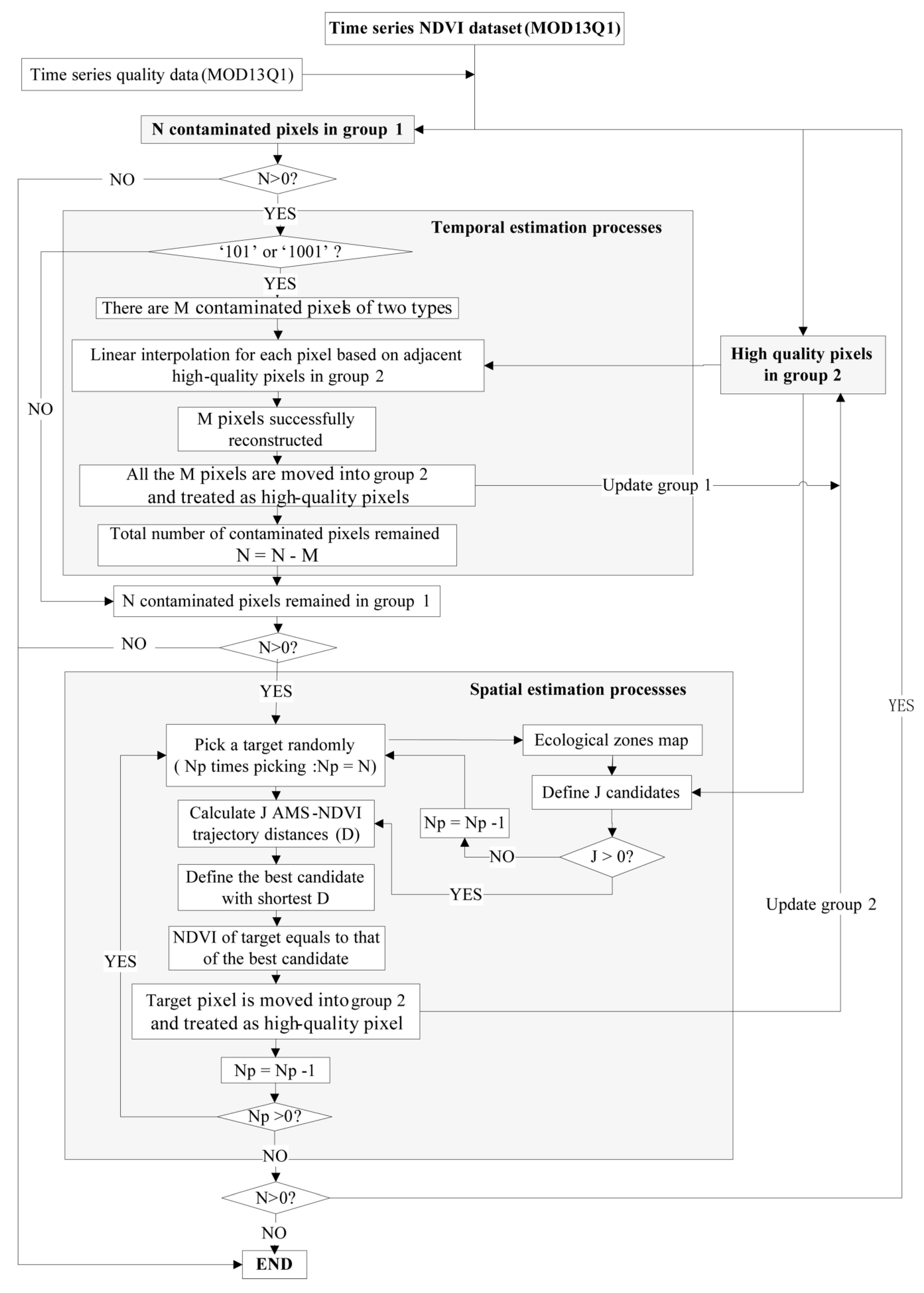
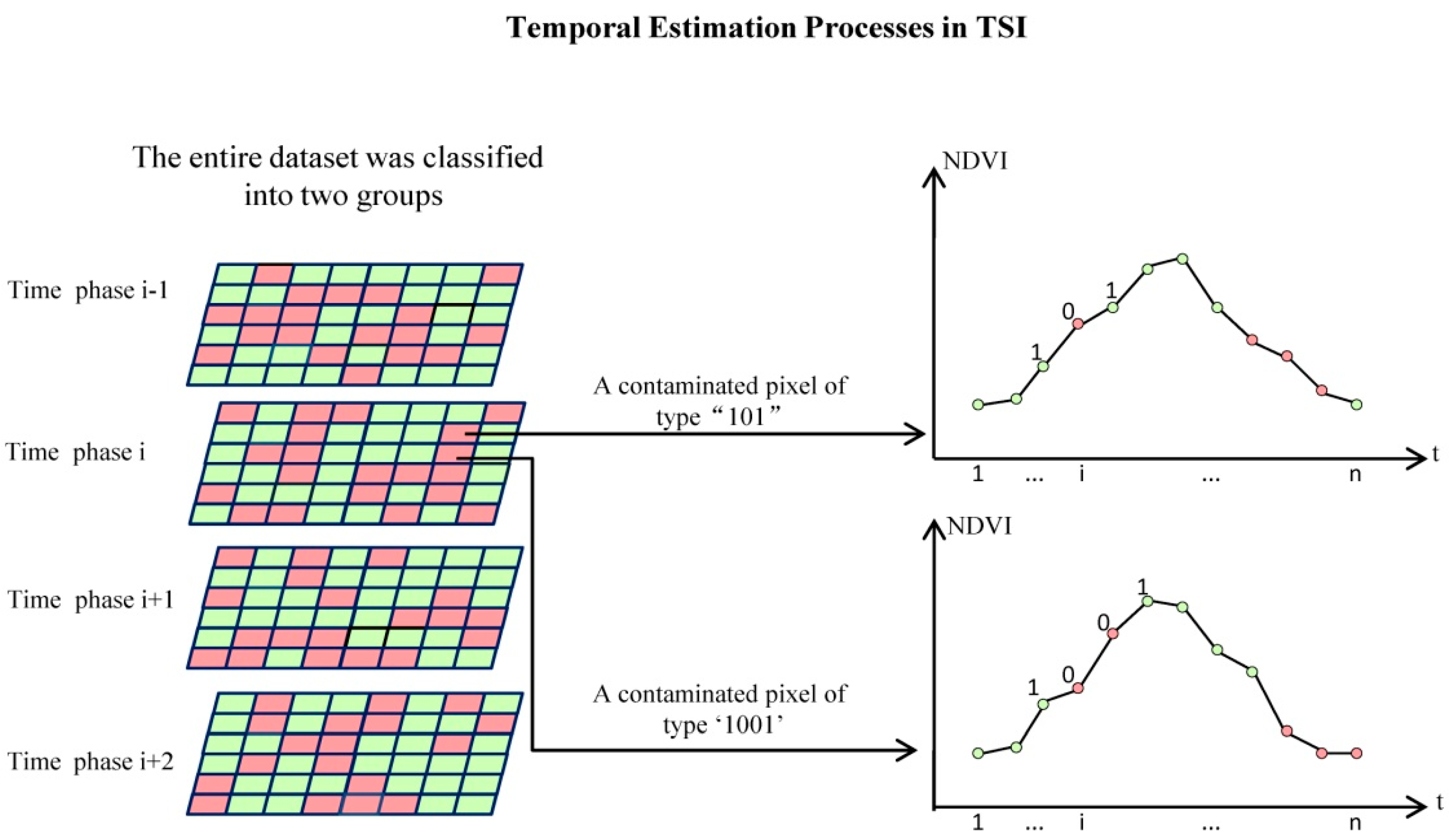
The estimation of the NDVIs of contaminated pixels using the TSI method was based on both temporal and spatial estimations. The NDVIs of the contaminated pixels based on temporal estimation were computed through linear interpolation of adjacent high-quality pixels in the time series. To reduce the impact of fluctuations due to vegetation growth, the contaminated NDVIs were only estimated using NDVIs of high-quality pixels from within one month forwards or backwards.
For temporal estimation, we predicted the NDVI of contaminated pixels solely based on the NDVIs of this pixel in other time phases. For spatial estimation, we predicted the NDVI of contaminated pixels from those of other pixels. However, the vegetation heterogeneity of 250 m MODIS data made it difficult to find a pixel with the same land cover as a contaminated one. Generally, the land cover types of a pixel seldom change within one month and the status of vegetation should not vary greatly within one month, meaning linear interpolation of NDVI in the temporal domain was more reliable than spatial estimation.
Figure 2.
Framework of the TSI method.
Spatial estimation strategies were based on the NDVI of high-quality pixels that contained similar land cover types, as established by Gao
et al. [
26] and Zhu
et al. [
27]. In this study, determining the most similar candidate pixel was not based directly on land cover maps because it was difficult to obtain a land cover map with high spatial accuracy. We assumed that the pixels with more similar NDVI change trajectories occupied more similar land cover types. Thus, the WTD algorithm based on the shortest NDVI trajectory distance was used to determine the pixel with the most similar land cover type for a contaminated pixel (details are shown in
Section 2.3.2).
2.3.2. Spatial Estimation
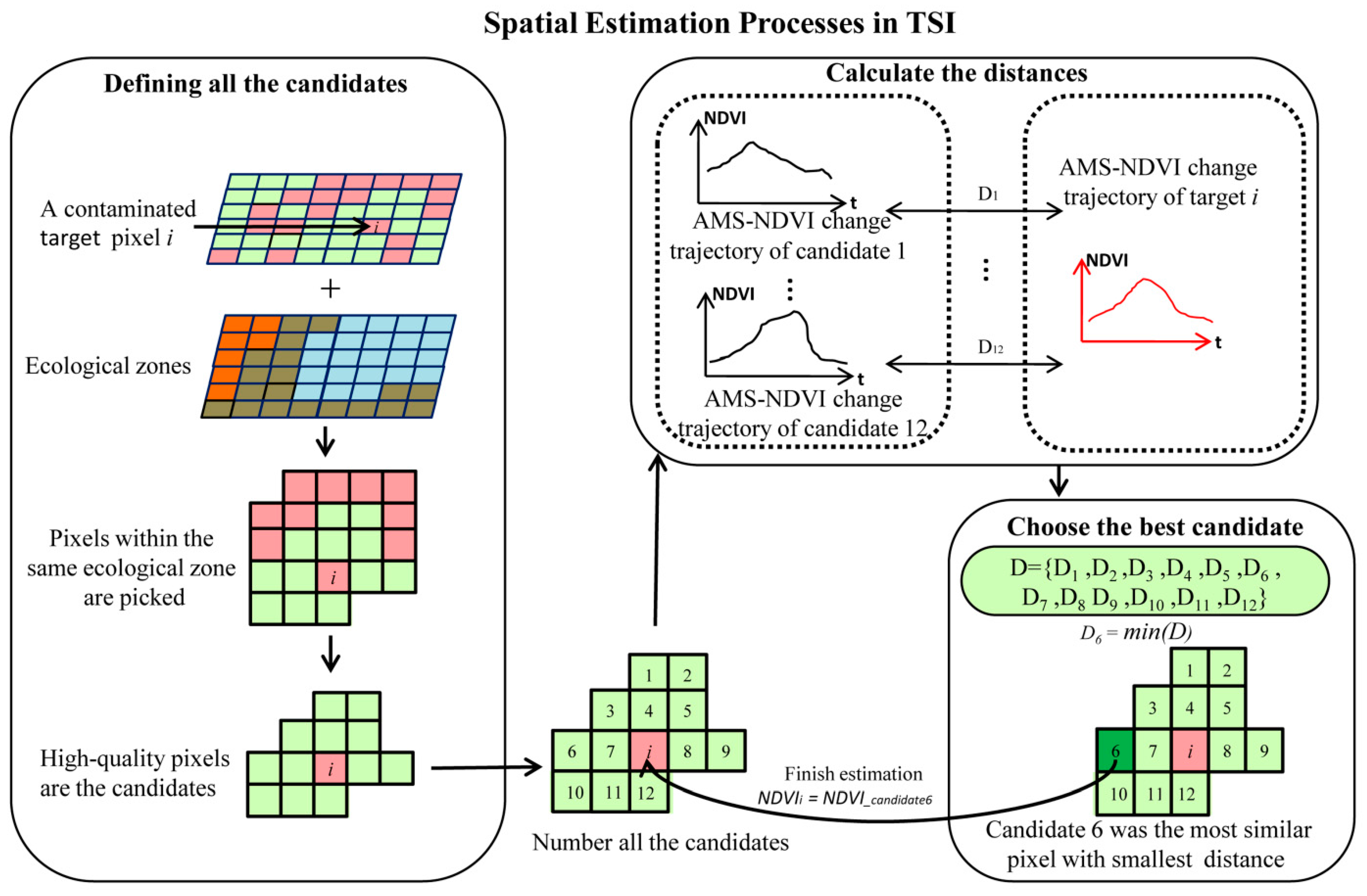
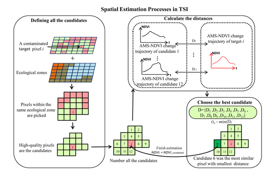
Step 1: defining all the candidates used for a contaminated NDVI estimation
This step is conducted to find all the suitable candidate pixels that can be used for the estimation of the contaminated NDVIs. For a contaminated NDVI, the candidates must satisfy three conditions, namely: (1) be pixels of high quality; (2) be in the same time phase as the contaminated pixel; and (3) be in the same ecological zone as the contaminated pixel (
Figure 4).
Figure 4.
Graphical representation of spatial neighborhood estimation.
Figure 4.
Graphical representation of spatial neighborhood estimation.
Step 2: calculating similarities of AMS-NDVI change trajectories between a target-contaminated NDVI and the candidates used for its estimation
For vegetation growth, the NDVIs in some key phases are important for controlling the form of the AMS-NDVI trajectory. Therefore, in this study, we selected the WTD to indicate the similarity of the AMS-NDVI change trajectory between a contaminated NDVI and the candidate used for its estimation. The WTD method assigns different weights to points within a change trajectory to measure the importance of points in affecting the form of the trajectory [
28,
29,
30]. The WTD can be calculated using Equation (4):
where
i is the
ith target contaminated pixel to be estimated,
j is the
jth high-quality candidate pixel used for the spatial neighborhood estimation,
n is the total number of time phases in the AMS-NDVI trajectory of the reconstructed NDVI series (
n = 12 in this paper),
is the trajectory distance between the
ith target and the
jth candidate, and
means the weight assigned to the
kth time phase in the growing season.
In this study, all the phases in a vegetation change trajectory were grouped into two classes: (1) key phases; and (2) non-key phases. Key phases (peak point, the fastest growth phase before peak point and the fastest decrease phase after peak point) controlled the fundamental form of the NDVI change trajectory and all other phases were considered as non-key phases. When
was calculated, the
for each key phase was given additional weight. The total of the additional weights equaled 1.0, and higher NDVI slope changes indicated higher weights. The value of
can be calculated using Equation (5):
where
is the weight of the NDVI in the
kth time phase;
is the additional weight in the
kth phase; and
m1,
m2, and
m3 are the time phases of the key phases (
Figure 4).
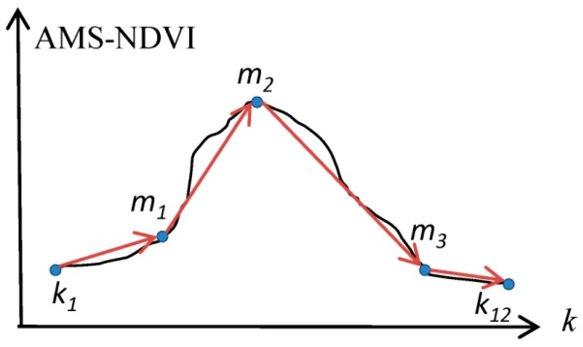
Figure 5.
The AMS-NDVI change trajectories with three key phases.
Figure 5.
The AMS-NDVI change trajectories with three key phases.
In this study, we used three key phases as the controls of the fundamental form of the AMS-NDVI change trajectory. The key phases were located at the peak period (
m2 in
Figure 5), start period (
m1 in
Figure 5), and end period (
m3 in
Figure 5),
i.e., where the NDVI changed most rapidly. The key phase in the peak period was the phase with maximum NDVI among all the NDVIs. The key phases in the start and end periods were determined as follows: (1) the change of NDVI slope for every phase on the growing part of the NDVI change trajectory before the peak or on the decreasing part after the peak was computed; (2) the phases where the change of NDVI slope was the greatest on the growing part of the NDVI change trajectory before the peak and on the decreasing part after the peak were selected as key phases. The additional weights for three key phases were computed using Equations (6) and (7):
where
is the additional weight in the
kth time phase,
k is the
kth time phase,
m1,
m2, and
m3 are the time phases of the key phases,
is the NDVI change slope between the 1st time phase (the first phase in the growing season) and the
time phase,
is the NDVI change slope between the
time phase and the
time phase,
is the NDVI change slope between the
time phase and the
time phase, and
is the NDVI change slope between the
time phase and the
nth time phase (final phase in the growing season) in the AMS-NDVI change trajectories.
is the total slope change in three key phases (
k = m1,
m2,
m3).
Step 3: choosing the best candidate and estimating the NDVI of a contaminated pixel
For an undetermined NDVI of a contaminated pixel, the most similar candidate was determined using Equation (8):
where
is the trajectory distance between the
ith contaminated pixel and the
jth candidate of the high-quality pixels for the estimation, and
is the shortest trajectory distance.
The undetermined NDVI was estimated based on the NDVI of the candidate shown as having the shortest trajectory distance by Equation (9):
where
is the estimated NDVI, and
is the NDVI of the candidate with the shortest trajectory distance among those between the estimated NDVI and all the candidates used for the estimation.
Step 4: iteration of temporal–spatial estimation of the NDVI of contaminated pixels
It is possible that some contaminated pixels will not be estimated following both the temporal and the spatial estimations. In such cases, the estimation process (steps 1–4 in
Section 2.3.2) is repeated, incorporating all the successfully estimated NDVIs of contaminated pixels as high-quality pixels. This iterative process continues until all the NDVIs of the contaminated pixels have been successfully estimated.


