
Large-Area Landslides Monitoring Using Advanced Multi-Temporal InSAR Technique over the Giant Panda Habitat, Sichuan, China


 ,
,
Abstract
:
1. Introduction
2. Study Area and Data
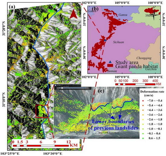
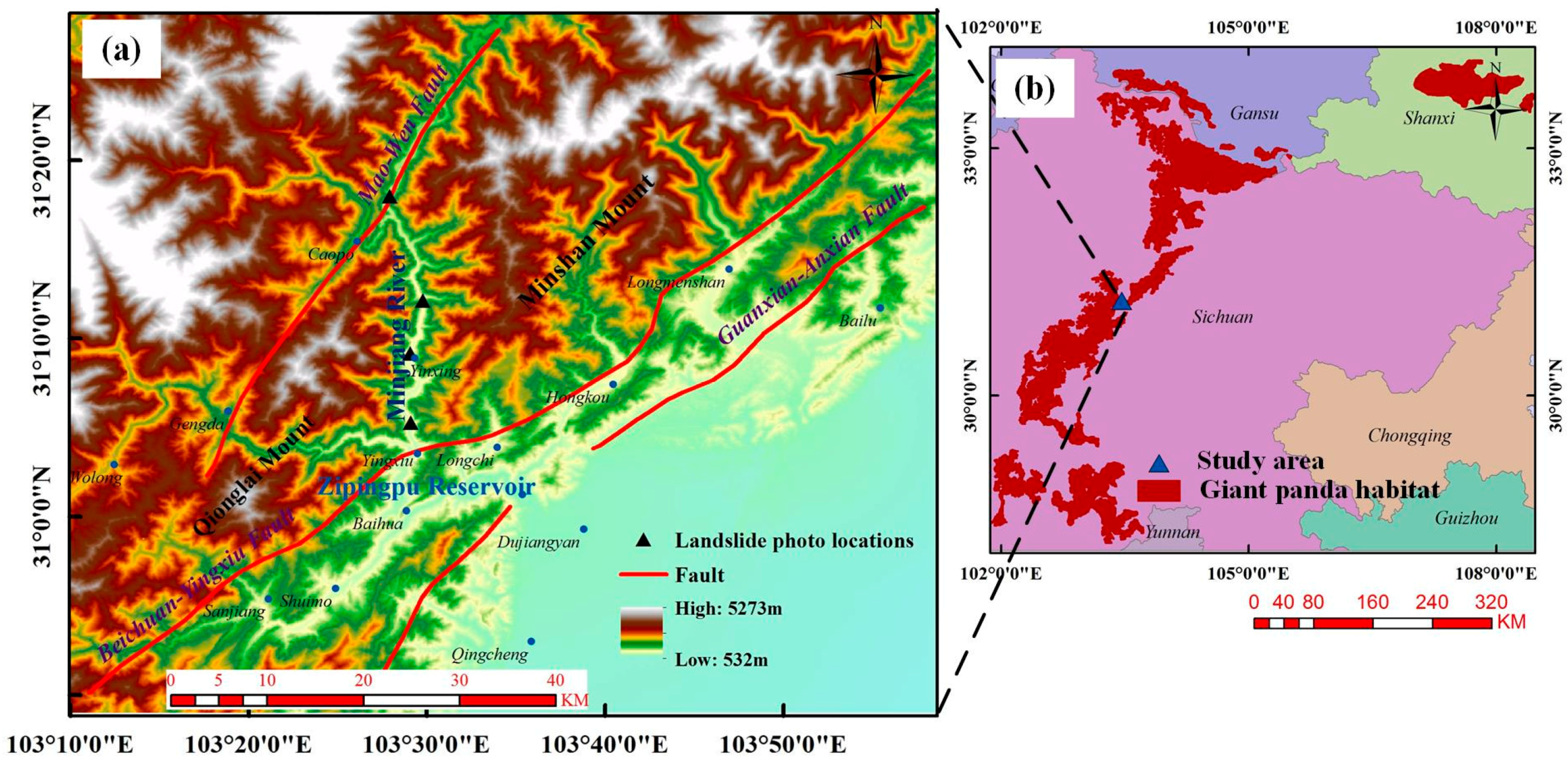
2.1. Study Site
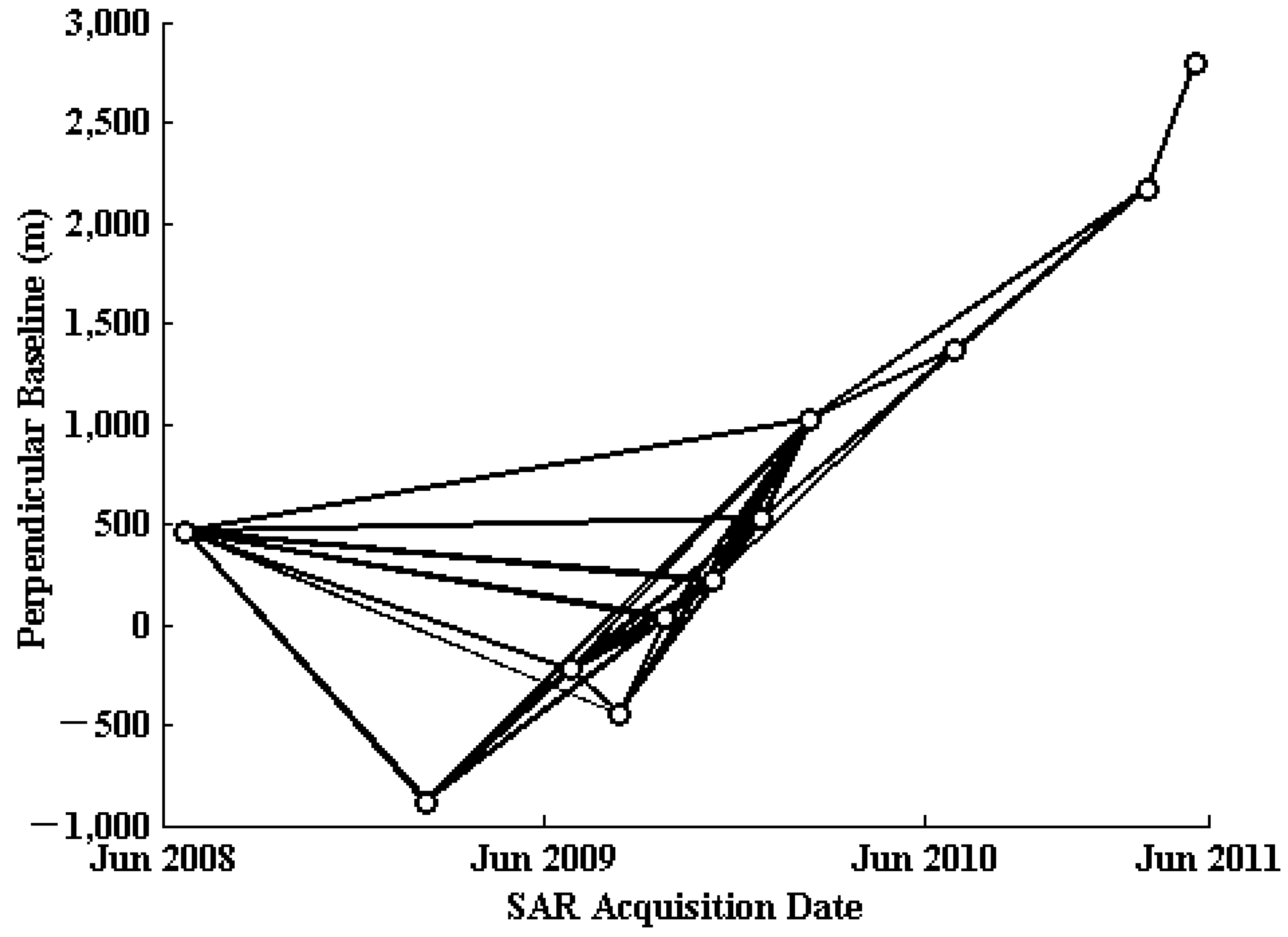
2.2. Data

| No. | Acquisition Time (yyyymmdd) | Polarization | Perpendicular Baseline (m) | Temporal Baseline (days) |
|---|---|---|---|---|
| 1 | 20080622 | HH | 244.8 | −506 |
| 2 | 20090207 | HH | −1102.5 | −276 |
| 3 | 20090625 | HH/HV | −439.5 | −138 |
| 4 | 20090810 | HH/HV | −662.9 | −92 |
| 5 | 20090925 | HH/HV | −184.1 | −46 |
| 6 | 20091110 | HH | 0 | 0 |
| 7 | 20091226 | HH | 316.2 | 46 |
| 8 | 20100210 | HH | 807.6 | 92 |
| 9 | 20100628 | HH/HV | 1157.7 | 230 |
| 10 | 20101229 | HH/HV | 1954.1 | 414 |
| 11 | 20110213 | HH | 2573.3 | 460 |
3. Methodology
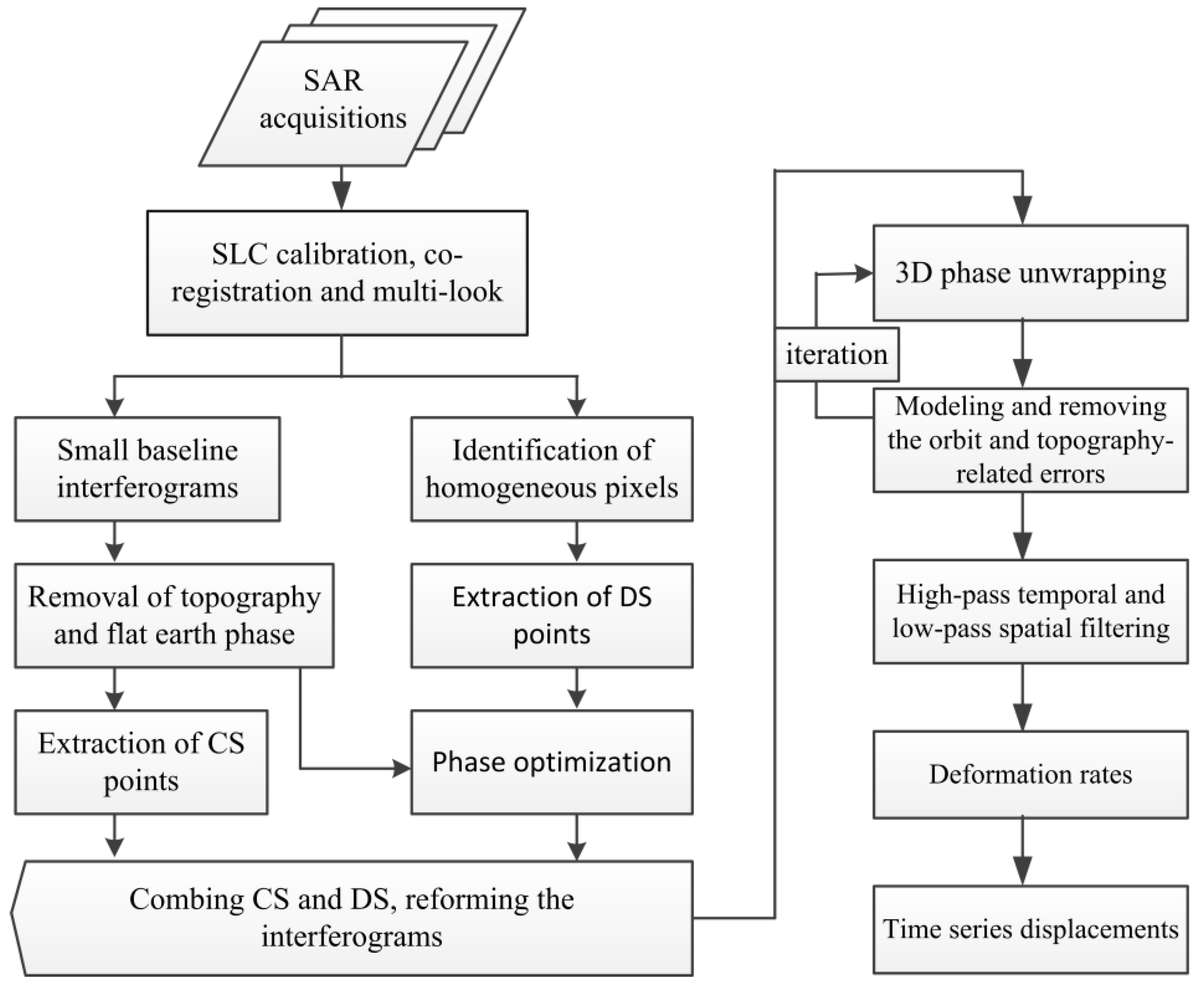
3.1. Combination of CS and DS


3.2. Parameter Estimation by SBAS Solution
3.3. Improvements and Advantages
4. Results, Validation and Discussion
4.1. Application to Landslide Monitoring


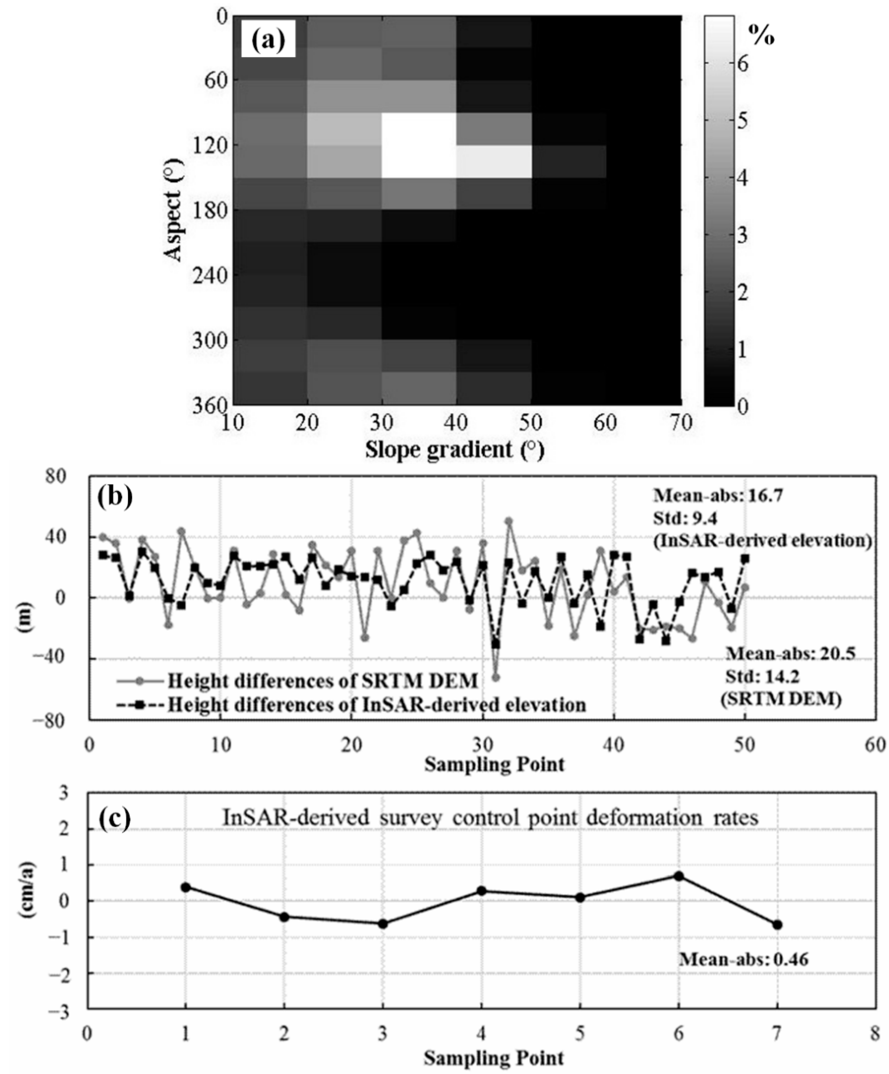
4.2. Validation
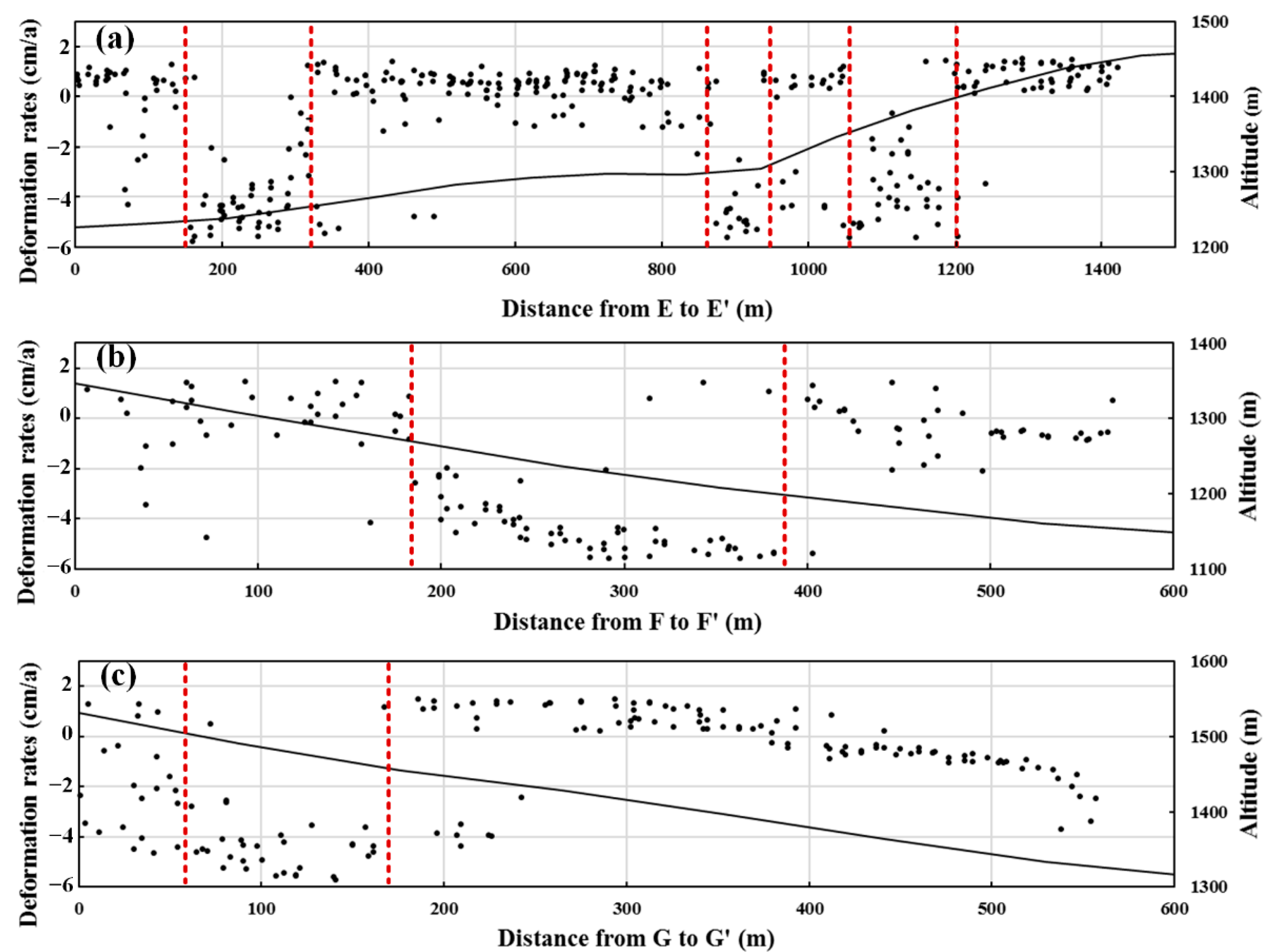
4.3. Deformation and Landslides Analysis
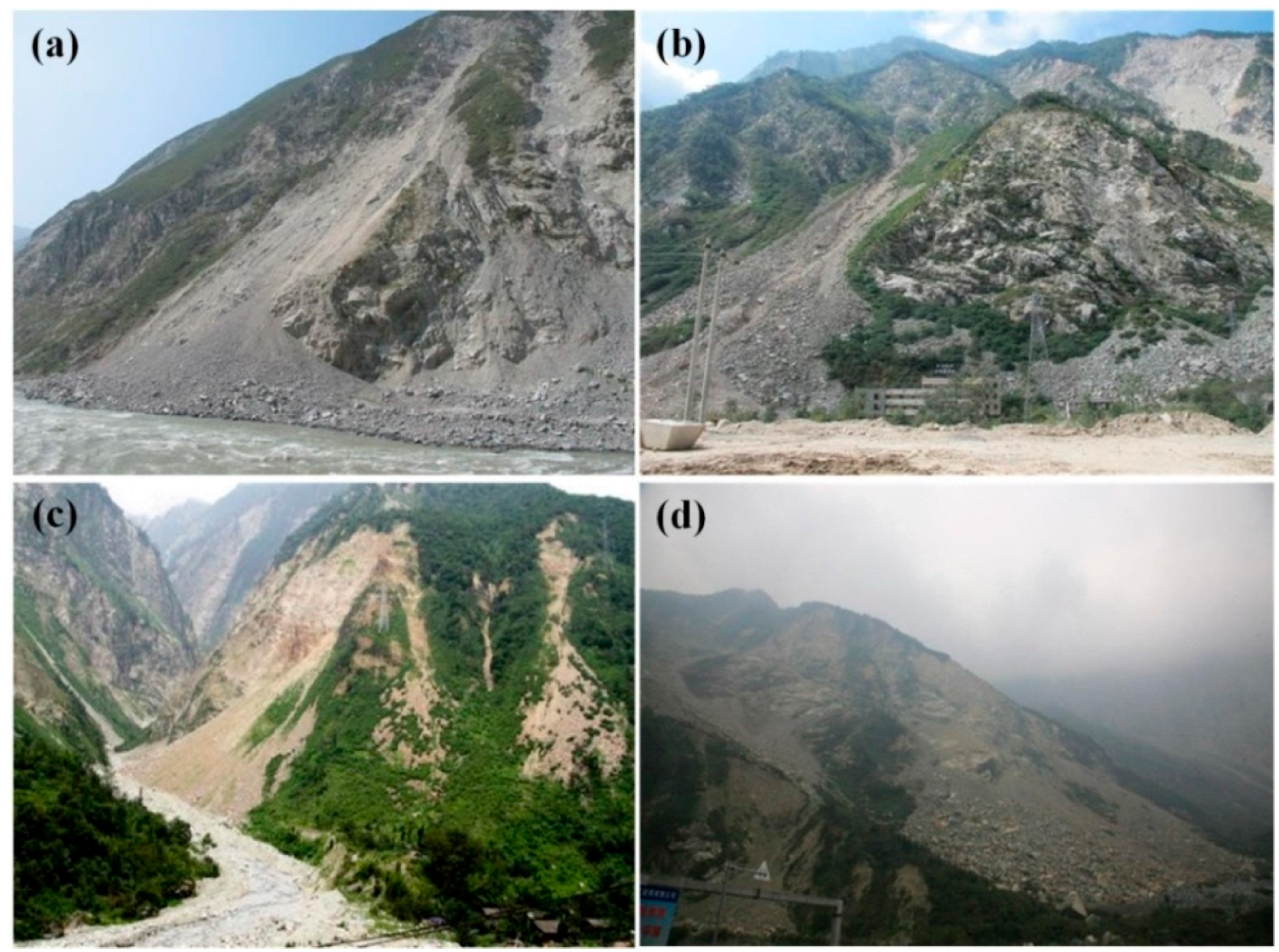
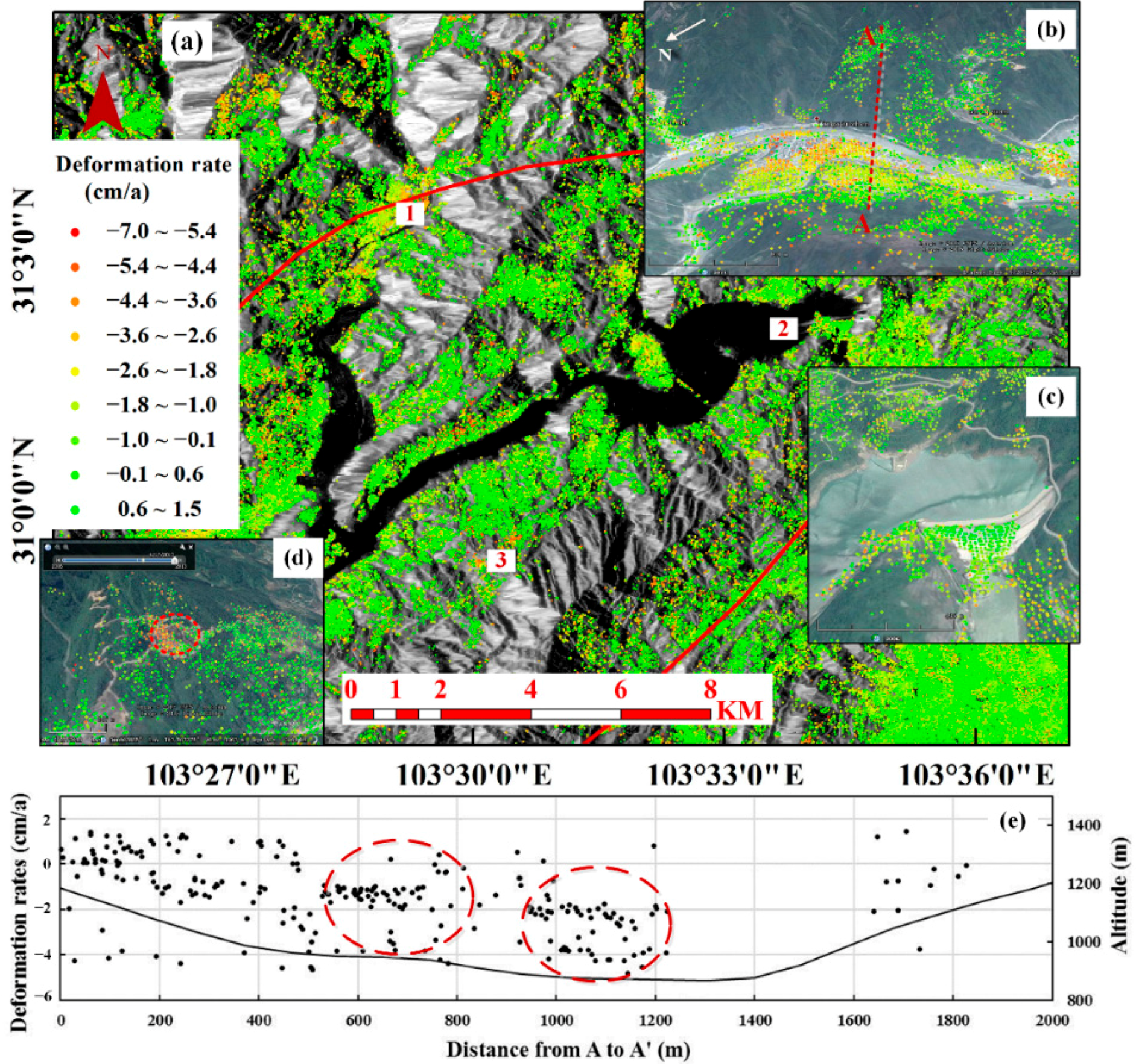
4.3.1. Minjiang River
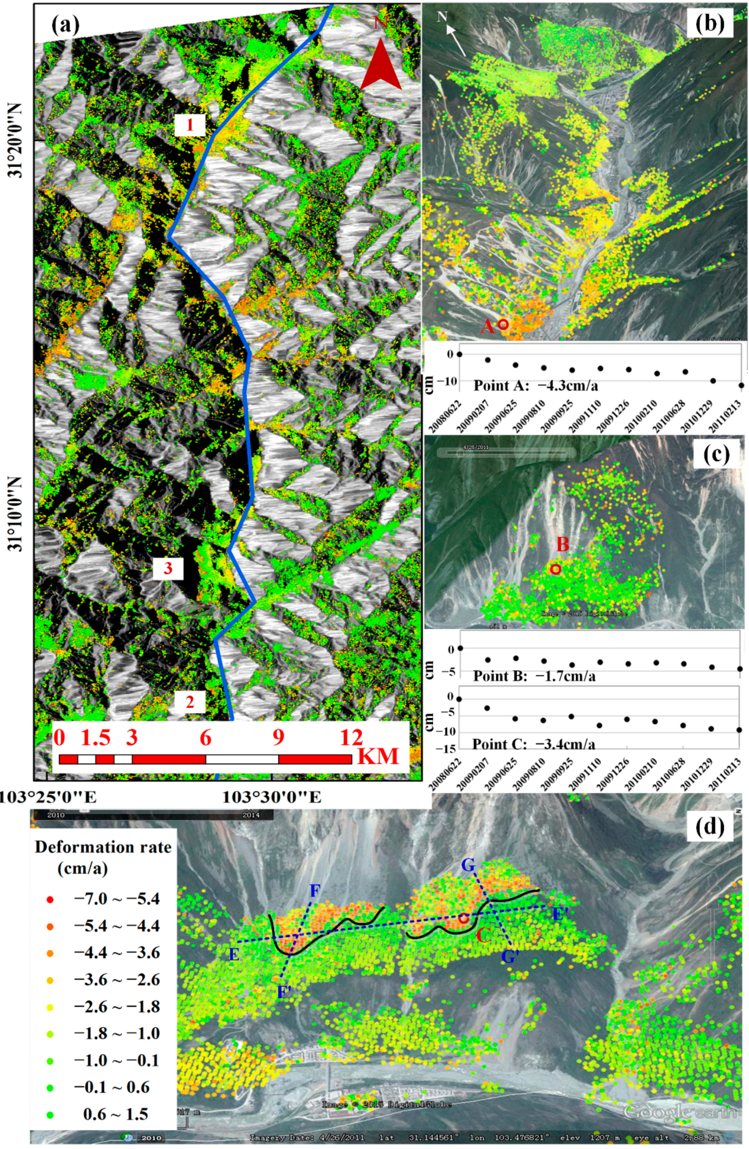

4.3.2. Longmenshan Fault
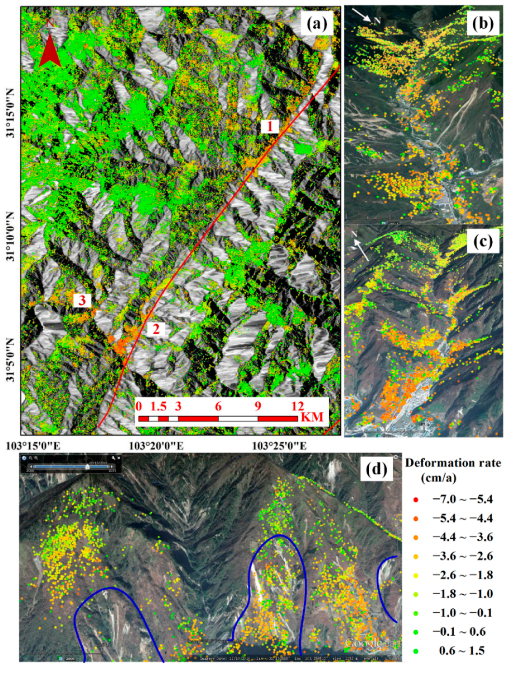

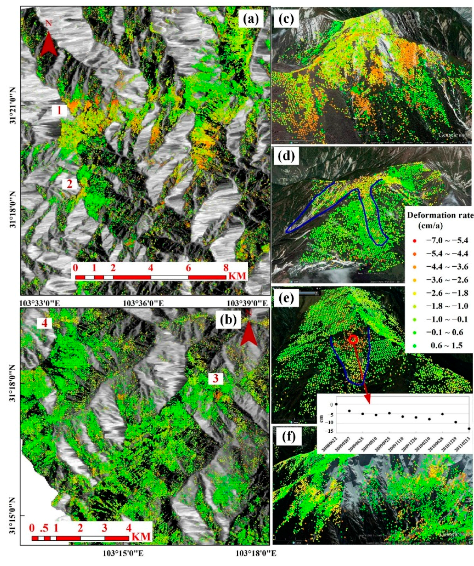
4.3.3. High-Altitude Mountains
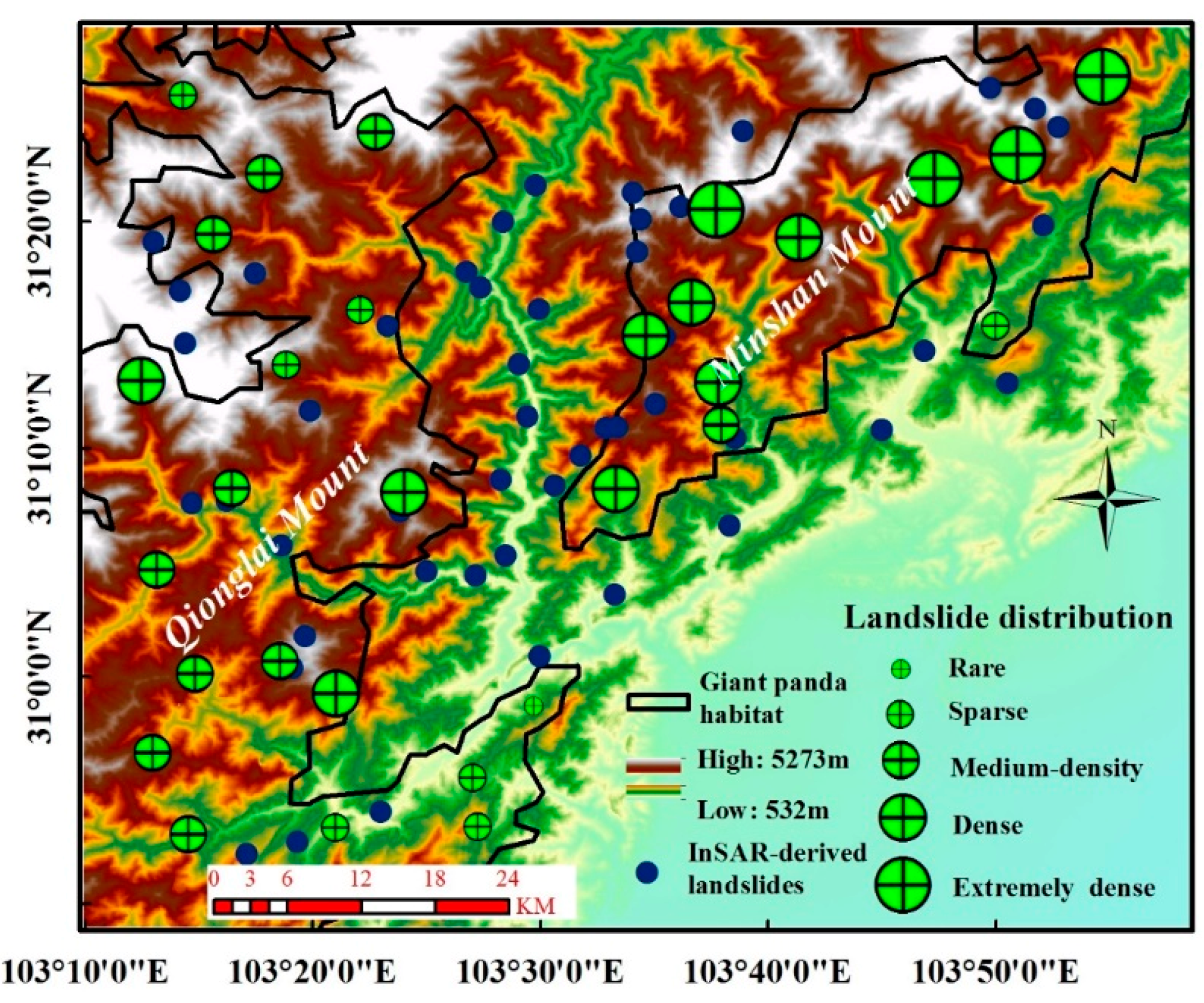
4.3.4. Giant Panda Habitat
5. Conclusions
Acknowledgments
Author Contributions
Conflicts of Interest
References
- Cruden, D.; Varnes, M.; David, J. Landslides: Investigation and mitigation. Chapter 3—Landslide types and processes. In Transportation Research Board Special Report; Transportation Research Board: Washington, DC, USA, 1996; pp. 36–75. [Google Scholar]
- Wu, Y.; He, S.M.; Li, X.P. Characteristics, causes and prevention measures of the landslides in Sichuan Province. J. Anhui Agric. Sci. 2008, 36, 7387–7390. [Google Scholar]
- Cui, P.; Zhu, Y.Y.; Han, Y.S.; Chen, X.Q.; Zhuang, J.Q. The 12 May Wenchuan earthquake-induced landslide lakes: Distribution and preliminary risk evaluation. Landslides 2009, 6, 209–223. [Google Scholar] [CrossRef]
- Dai, F.C.; Xu, C.; Yao, X.; Xu, L.; Tu, X.B.; Gong, Q.M. Spatial distribution of landslides triggered by the 2008 Ms 8.0 Wenchuan earthquake, China. J. Asian Earth Sci. 2011, 40, 883–895. [Google Scholar] [CrossRef]
- Huang, R.Q.; Li, W.L. Post-earthquake landsliding and long-term impacts in the Wenchuan earthquake area, China. Eng. Geol. 2014, 182, 111–120. [Google Scholar] [CrossRef]
- Dai, F.C.; Lee, C.F.; Ngai, Y.Y. Landslide risk assessment and management: An overview. Eng. Geol. 2002, 64, 65–87. [Google Scholar] [CrossRef]
- Chen, F.L.; Lin, H.; Hu, X. Slope superficial displacement monitoring by small baseline SAR interferometry using data from L-band ALOS PALSAR and X-band TerraSAR: A case study of Hong Kong, China. Remote Sens. 2014, 6, 1564–1586. [Google Scholar] [CrossRef]
- Thompson, P.W.; Cierlitza, S. Identification of a slope failure over a year before final collapse using multiple monitoring. In Geotechnical Instrumentation and Monitoring in Open Pit and Underground Mining; Szwedzicki, T., Ed.; CRC Press: Boca Raton, FL, USA, 1993; pp. 491–511. [Google Scholar]
- Massonnet, D.; Feigl, K.L. Radar interferometry and its application to changes in the Earth’s surface. Rev. Geophys. 1998, 36, 441–500. [Google Scholar] [CrossRef]
- Bovenga, F.; Nitti, D.O.; Refice, A.; Nutricato, R.; Chiaradia, M.T. Multi-temporal DInSAR analysis with X-band high-resolution SAR data: Examples and potential. In Proceedings of the SPIE 78290I-78290I-10 (2010); SAR Image Analysis, Modeling, and Techniques X, Toulouse, France, 20–23 September 2010.
- Fruneau, B.; Achace, J.; Delacourt, C. Observation and modeling of the Saint-Etienne-de-Tinée landslide using SAR interferometry. Tectonophysics 1996, 265, 181–190. [Google Scholar] [CrossRef]
- Ferretti, A.; Prati, C.; Rocca, F. Permanent scatterers in SAR interferometry. IEEE Trans. Geosci. Remote Sens. 2001, 39, 8–20. [Google Scholar] [CrossRef]
- Berardino, P.; Fornaro, G.; Lanari, R.; Sansosti, E. A new algorithm for surface deformation monitoring based on small baseline differential SAR interferograms. IEEE Trans. Geosci. Remote Sens. 2002, 40, 2375–2383. [Google Scholar] [CrossRef]
- Ferretti, A.; Fumagalli, A.; Novali, F.; Prati, C.; Rocca, F.; Rucci, A. A new algorithm for processing interferometric data-stacks: SqueeSAR. IEEE Trans. Geosci. Remote Sens. 2011, 49, 3460–3470. [Google Scholar] [CrossRef]
- Bovenga, F.; Wasowski, J.; Nitti, D.O.; Nutricato, R.; Chiaradia, M.T. Using COSMO/SkyMed X-band and ENVISAT C-band SAR interferometry for landslides analysis. Remote Sens. Environ. 2012, 119, 272–285. [Google Scholar] [CrossRef]
- Cascini, L.; Fornaro, G.; Peduto, D. Advanced low- and full-resolution DInSAR map generation for slow-moving landslide analysis at different scales. Eng. Geol. 2010, 112, 29–42. [Google Scholar] [CrossRef]
- Colesanti, C.; Ferretti, A.; Prati, C.; Rocca, F. Monitoring landslides and tectonic motion with the permanent scatterers technique. Eng. Geol. 2003, 68, 3–14. [Google Scholar] [CrossRef]
- Colesanti, C.; Wasowski, J. Investigating landslides with space-borne synthetic aperture radar (SAR) interferometry. Eng. Geol. 2006, 88, 173–199. [Google Scholar] [CrossRef]
- Calò, F.; Ardizzone, F.; Castaldo, R.; Lollino, P.; Tizzani, P.; Guzzetti, F.; Lanari, R.; Angeli, M.; Pontoni, F.; Manunta, M. Enhanced landslide investigations through advanced DInSAR techniques: The Ivancich case study, Assisi, Italy. Remote Sens. Environ. 2014, 142, 69–82. [Google Scholar] [CrossRef]
- Farina, P.; Colombo, D.; Fumagalli, A.; Marks, F.; Moretti, S. Permanent Scatterers for landslide investigations: Outcomes from the ESA-SLAM project. Eng. Geol. 2006, 88, 200–217. [Google Scholar] [CrossRef]
- Herrera, G.; Gutiérrez, F.; García-Davalillo, J.C.; Guerrero, J.; Notti, D.; Galve, J.P.; Cooksley, G.; Fernández-Merodo, J.A. Multi-sensor advanced DInSAR monitoring of very slow landslides: The Tena Valley case study (Central Spanish Pyrenees). Remote Sens. Environ. 2013, 128, 31–43. [Google Scholar] [CrossRef]
- Hilley, G.E.; Burgmann, R.; Ferretti, A.; Novali, F.; Rocca, F. Dynamics of slow-moving landslides from permanent scatterer analysis. Science 2004, 304, 1952–1955. [Google Scholar] [CrossRef] [PubMed]
- Liu, P.; Li, Z.; Hoey, T.; Kincal, C.; Zhang, J.; Zeng, Q.; Muller, J.P. Using advanced InSAR time series techniques to monitor landslide movements in Badong of the Three Gorges region, China. Int. J. Appl. Earth Obs. 2013, 21, 253–264. [Google Scholar] [CrossRef]
- Del Ventisette, C.; Righini, G.; Moretti, S.; Casagli, N. Multitemporal landslides inventory map updating using spaceborne SAR analysis. Int. J. Appl. Earth Obs. 2014, 30, 238–246. [Google Scholar] [CrossRef]
- Hanssen, R.F. Radar interferometry: Data Interpretation and Error Analysis (Vol. 2); Springer Science & Business Media: Dordrecht, The Netherlands, 2001. [Google Scholar]
- Samsonov, S.; van der Kooij, M.; Tiampo, K. A simultaneous inversion for deformation rates and topographic errors of DInSAR data utilizing linear least square inversion technique. Comput. Geosci. 2011, 37, 1083–1091. [Google Scholar] [CrossRef]
- Yun, S.H.; Zebker, H.A.; Segall, P.; Hooper, A.; Poland, M. Interferogram formation in the presence of complex and large deformation. Geophys. Res. Lett. 2007, 34, 237–254. [Google Scholar] [CrossRef]
- Lauknes, T.R. InSAR tropospheric stratification delays: Correction using a small baseline approach. IEEE Geosci. Remote Sens. Lett. 2011, 8, 1070–1074. [Google Scholar] [CrossRef]
- Zebker, H.A.; Rosen, P.A.; Hensley, S. Atmospheric effects in interferometric synthetic aperture radar surface deformation and topographic maps. J. Geophys. Res. 1997, 102, 7547–7563. [Google Scholar] [CrossRef]
- Wasowski, J.; Bovenga, F. Investigating landslides and unstable slopes with satellite Multi Temporal Interferometry: Current issues and future perspectives. Eng. Geol. 2014, 174, 103–138. [Google Scholar] [CrossRef]
- Chigira, M.; Wu, X.; Inokuchi, T.; Wang, G. Landslides induced by the 2008 Wenchuan earthquake, Sichuan, China. Geomorphology 2010, 118, 225–238. [Google Scholar] [CrossRef]
- Fan, X.; van Westen, C.J.; Xu, Q.; Gorum, T.; Dai, F. Analysis of landslide dams induced by the 2008 Wenchuan earthquake. J. Asian Earth Sci. 2012, 57, 25–37. [Google Scholar] [CrossRef]
- Gorum, T.; Fan, X.; van Westen, C.J.; Huang, R.Q.; Xu, Q.; Tang, C.; Wang, G.H. Distribution pattern of earthquake-induced landslides triggered by the 12 May 2008 Wenchuan earthquake. Geomorphology 2011, 133, 152–167. [Google Scholar] [CrossRef]
- Huang, R.Q.; Li, W.L. Development and distribution of geohazards triggered by the 5.12 Wenchuan Earthquake in China. Sci. China Ser. E 2009, 52, 810–819. [Google Scholar] [CrossRef]
- Strozzi, T.; Farina, P.; Corsini, A.; Ambrosi, C.; Thüring, M.; Zilger, J.; Wiesmann, A.; Wegmüller, U.; Werner, C. Survey and monitoring of landslide displacements by means of L-band satellite SAR interferometry. Landslides 2005, 2, 193–201. [Google Scholar] [CrossRef]
- García-Davalillo, J.C.; Herrera, G.; Notti, D.; Strozzi, T.; Álvarez-Fernández, I. DInSAR analysis of ALOS PALSAR images for the assessment of very slow landslides: The Tena Valley case study. Landslides 2014, 11, 225–246. [Google Scholar] [CrossRef]
- Zhao, C.Y.; Lu, Z.; Zhang, Q.; de La Fuente, J. Large-area landslide detection and monitoring with ALOS/PALSAR imagery data over Northern California and Southern Oregon, USA. Remote Sens. Environ. 2012, 124, 348–359. [Google Scholar] [CrossRef]
- Zhang, Y.; Cheng, Y.; Yin, Y.; Lan, H.; Wang, J.; Fu, X. High-position debris flow: A long-term active geohazard after the Wenchuan earthquake. Eng. Geol. 2014, 180, 45–54. [Google Scholar] [CrossRef]
- Handwerger, A.L.; Roering, J.J.; Schmidt, D.A. Controls on the seasonal deformation of slow-moving landslides. Earth Planet. Sci. Lett. 2013, 377, 239–247. [Google Scholar] [CrossRef]
- Chen, F.L.; Guo, H.D.; Ishwaran, N.; Zhou, W.; Yang, R.X.; Jing, L.H.; Chen, F.; Zeng, H.C. Synthetic aperture radar (SAR) interferometry for assessing Wenchuan earthquake (2008) deforestation in the Sichuan giant panda site. Remote Sens. 2014, 6, 6283–6299. [Google Scholar] [CrossRef]
- Wang, X.; Xu, W.; Ouyang, Z.; Zhang, J. Impacts of Wenchuan Earthquake on giant panda habitat in Dujiangyan region. Acta Ecol. Sin. 2008, 28, 5856–5861. [Google Scholar]
- Jarvis, A.; Reuter, H.I.; Nelson, A.; Guevara, E. Hole-filled SRTM for the globe Version 4, Available from the CGIAR-CSI SRTM 90 m Database. 2008. Available online: http://srtm.csi.cgiar.org (accessed on 8 July 2015).
- Monti Guarnieri, A.; Tebaldini, S. A new framework for multi-pass SAR interferometry with distributed targets. In Proceedings of the IGARSS 2007, Barcelona, Spain, 23–28 July 2007; pp. 5289–5293.
- Lv, X.; Yazici, B.; Zeghal, M.; Bennett, V.; Abdoun, T. Joint-scatterer processing for time-series InSAR. IEEE Trans. Geosci. Remote Sens. 2014, 52, 7205–7221. [Google Scholar]
- Deledalle, C.A.; Denis, L.; Tupin, F.; Reigber, A.; Jager, M. NL-SAR: A unified nonlocal framework for resolution-preserving (Pol) (In) SAR Denoising. IEEE Trans. Geosci. Remote Sens. 2015, 53, 2021–2037. [Google Scholar] [CrossRef]
- Vasile, G.; Trouvé, E.; Lee, J.S.; Buzuloiu, V. Intensity-driven adaptive-neighborhood technique for polarimetric and interferometric SAR parameters estimation. IEEE Trans. Geosci. Remote Sens. 2006, 44, 1609–1621. [Google Scholar] [CrossRef]
- Liu, D.; Nocedal, J. On the limited memory method for large scale optimization. Math. Program. 1989, 45, 503–528. [Google Scholar] [CrossRef]
- Byrd, R.H.; Lu, P.; Nocedal, J.; Zhu, C. A limited memory algorithm for bound constrained optimization. SIAM J. Sci. Stat. Comput. 1995, 16, 1190–1208. [Google Scholar] [CrossRef]
- Pepe, A.; Lanari, R. On the extension of the minimum cost flow algorithm for phase unwrapping of multitemporal differential SAR interferograms. IEEE Trans. Geosci. Remote Sens. 2006, 44, 2374–2383. [Google Scholar] [CrossRef]
- Nakamura, R.; Nakamura, S.; Kudo, N.; Katagiri, S. Precise orbit determination for ALOS. In Proceedings of the 20th International Symposium on Space Flight Dynamics, Annapolis, MD, USA, 24–28 September 2007.
- Goldstein, R. Atmospheric limitations to repeat-track radar interferometry. Geophys. Res. Lett. 1995, 22, 2517–2520. [Google Scholar] [CrossRef]
- Xu, B.; Li, Z.W.; Wang, Q.J.; Jiang, M.; Zhu, J.J.; Ding, X.L. A Refined Strategy for Removing Composite Errors of SAR Interferogram. IEEE Geosci. Remote Sens. Lett. 2014, 11, 143–147. [Google Scholar] [CrossRef]
- Shirzaei, M.; Walter, T.R. Estimating the effect of satellite orbital error using wavelet-based robust regression applied to InSAR deformation data. IEEE Trans. Geosci. Remote Sens. 2011, 49, 4600–4605. [Google Scholar] [CrossRef]
- Wegmüller, U.; Werner, C. Gamma SAR Processor and Interferometry Software. Available online: http://earth.esa.int/workshops/ers97/papers/wegmuller2/ (accessed on 8 July 2015).
- Chaabane, F.; Avallone, A.; Tupin, F.; Briole, P.; Maître, H. A multitemporal method for correction of tropospheric effects in differential SAR interferometry: Application to the Gulf of Corinth earthquake. IEEE Trans. Geosci. Remote Sens. 2007, 45, 1605–1615. [Google Scholar] [CrossRef]
- Sun, Q.; Zhang, L.; Ding, X.L.; Hu, J.; Li, Z.W.; Zhu, J.J. Slope deformation prior to Zhouqu, China landslide from InSAR time series analysis. Remote Sens. Environ. 2015, 156, 45–57. [Google Scholar] [CrossRef]
- Zwally, H.J.; Schutz, B.; Abdalati, W.; Abshire, J.; Bentley, C.; Brenner, A.; Bufton, J.; Dezio, J.; Hancock, D.; Harding, D.; et al. ICESat’s laser measurements of polar ice, atmosphere, ocean, and land. J. Geodyn. 2002, 34, 405–445. [Google Scholar] [CrossRef]
- State Forestry Administration. The Third National Survey Report on the Giant Panda in China; Science Press: Beijing, China, 2006. (In Chinese)
- Ouyang, Z.Y.; Xu, W.H.; Wang, X.Z.; Wang, W.J.; Dong, R.C.; Zheng, H.; Li, D.H.; Li, Z.Q.; Zhang, H.F.; Zhuang, C.W. Impact assessment of Wenchuan earthquake on ecosystems. Acta Ecol. Sin. 2008, 28, 5856–5861. [Google Scholar]
- Shen, G.Z.; Xie, Z.Q.; Feng, C.Y.; Xu, W.T.; Guo, K. Influence of the Wenchuan earthquake on giant panda habitats and strategies for restoration. J. Plant Ecol. Chin. Version 2008, 32, 1417–1425. [Google Scholar]
© 2015 by the authors; licensee MDPI, Basel, Switzerland. This article is an open access article distributed under the terms and conditions of the Creative Commons Attribution license (http://creativecommons.org/licenses/by/4.0/).
Share and Cite
Tang, P.; Chen, F.; Guo, H.; Tian, B.; Wang, X.; Ishwaran, N. Large-Area Landslides Monitoring Using Advanced Multi-Temporal InSAR Technique over the Giant Panda Habitat, Sichuan, China. Remote Sens. 2015, 7, 8925-8949. https://doi.org/10.3390/rs70708925
Tang P, Chen F, Guo H, Tian B, Wang X, Ishwaran N. Large-Area Landslides Monitoring Using Advanced Multi-Temporal InSAR Technique over the Giant Panda Habitat, Sichuan, China. Remote Sensing. 2015; 7(7):8925-8949. https://doi.org/10.3390/rs70708925
Chicago/Turabian StyleTang, Panpan, Fulong Chen, Huadong Guo, Bangsen Tian, Xinyuan Wang, and Natarajan Ishwaran. 2015. "Large-Area Landslides Monitoring Using Advanced Multi-Temporal InSAR Technique over the Giant Panda Habitat, Sichuan, China" Remote Sensing 7, no. 7: 8925-8949. https://doi.org/10.3390/rs70708925
APA StyleTang, P., Chen, F., Guo, H., Tian, B., Wang, X., & Ishwaran, N. (2015). Large-Area Landslides Monitoring Using Advanced Multi-Temporal InSAR Technique over the Giant Panda Habitat, Sichuan, China. Remote Sensing, 7(7), 8925-8949. https://doi.org/10.3390/rs70708925