Annual Detection of Forest Cover Loss Using Time Series Satellite Measurements of Percent Tree Cover


Abstract
: We introduce and test a new method to detect annual forest cover loss from time series estimates of percent tree cover. Our approach is founded on two realistic assumptions: (1) land cover disturbances are rare events over large geographic areas that occur within a short time frame; and (2) spatially discrete land cover disturbances are continuous processes over time. Applying statistically rigorous algorithms, we first detect disturbance pixels as outliers of an underlying chi-square distribution. Then, we fit nonlinear, logistic curves for each identified change pixel to simultaneously characterize the magnitude and timing of the disturbance. Our method is applied using the yearly Vegetation Continuous Fields (VCF) tree cover product from Moderate Resolution Imaging Spectroradiometer (MODIS), and the resulting disturbance-year estimates are evaluated using a large sample of Landsat-based forest disturbance data. Temporal accuracy is ∼65% at 250-m, annual resolution and increases to >85% when temporal resolution is relaxed to ±1 yr. The r2 of MODIS VCF-based disturbance rates against Landsat ranges from 0.7 to 0.9 at 5-km spatial resolution. The general approach developed in this study can be potentially applied at a global scale and to other land cover types characterized as continuous variables from satellite data.1. Introduction
Forest cover loss is releasing massive quantities of carbon dioxide from the terrestrial biosphere into the atmosphere [1]. As the second largest source of anthropogenic greenhouse gas emissions, tropical deforestation is estimated to emit 0.3 to 0.8 petagrams of carbon per year (Pg·C·yr−1) into the atmosphere in the 1980s, 0.5 to 3.0 Pg·C·yr−1 in the 1990s and 0.81 to 2.2 Pg·C·yr−1 in the 2000s [2–7]. The large range of emission estimates is mainly due to uncertainties in both deforestation and biomass density estimates [1,8]. A recent study suggested that areal estimates of deforestation could contribute as many as 5–10-times more error to emission estimates than biomass data [5]. The accurate quantification of forest cover change is therefore critically important for reducing uncertainties in carbon emission estimates and for evaluating the effectiveness of environmental policies aiming at reducing emissions from deforestation and forest degradation (REDD+).
Changes in forest and other land cover types have been monitored by various techniques using remotely sensed data for over four decades [9,10]. Although many successful applications of satellite monitoring of forest cover change are carried out at sparse temporal intervals (e.g., 5 yr, 10 yr or longer) [11–17], forest change rates have been shown to vary substantially from one year to another [18–20]. Hence, change products derived at sparse temporal intervals cannot capture such temporal dynamics, especially when forest cover change is caused by harvest and other land management practices [21]. In areas where forests can re-establish within a few years after having been cleared, coarse-interval change detection may also miss significant portions of the changes that are followed by rapid regrowth [14,22,23].
To overcome these limitations, a growing number of studies have exploited dense time series of satellite observations for monitoring forest cover change. In particular, a number of novel techniques have recently emerged for reconstructing forest change history using dense time series of Landsat images [24–27]. Consisting of “clear-view” Landsat observations every year or every two years [19], such image stacks allow forest change mapping at annual or biennial time steps. Although Landsat provides one of the longest and most consistent satellite records of the land surface with a spatial resolution suitable for monitoring many types of anthropogenic land cover change [28], dense time series of Landsat observations do not exist in many areas outside the U.S. [29]. So far, optimized global collections of Landsat images are available only for a few selected epochs centered at 1975, 1990, 2000, 2005 and 2010 [30–32], although global wall-to-wall coverage has been constructed using all available Landsat 7 Enhanced Thematic Mapper Plus (ETM+) images between 2000 and 2012 [20]. In the tropics, where most carbon emissions from deforestation are located, cloud and shadow contamination is another limiting factor for large-area land cover change mapping with Landsat [33]. Coarse-resolution sensors, such as MODIS, with a daily revisit frequency, have a greater probability of obtaining cloud-free observations annually [22,33].
Methods for mapping forest disturbance using time series satellite data mainly rely on detecting structural changes in the spectral responses of a pixel over time [26,27,34] or changes in spectral-based indices, such as the Normalized Difference Vegetation Index (NDVI) [35–37], Enhanced Vegetation Index (EVI) [38], disturbance index [14,39], MODIS global disturbance index [40], the integrated forest z-score [24], etc. Spectral index-based methods (e.g., NDVI) typically seek a drop in inter-annual signals to infer forest loss or an increase for forest gain. Whereas NDVI is a robust indicator of vegetation cover; even a strong drop in NDVI may not be unambiguously related to forest loss, as other vegetation changes, such as crop rotation, may result in similar patterns of NDVI change. Moreover, time series of vegetation indices are often sensitive to fluctuations in primary productivity and/or climatic fluctuations at intra-annual scales, causing difficulties for land cover change detection [41]. As an alternative, explicitly converting intra-annual satellite signals to annual continuous tree cover and then tracking year-to-year changes in tree cover provides another useful way for disturbance mapping [41,42].
The objective of this study is to develop and test a novel procedure to quantify annual forest cover loss using time series MODIS Vegetation Continuous Fields (VCF) tree cover dataset. The MODIS VCF product (MOD44B), currently in Collection 5, has a spatial resolution of 250-m and a temporal resolution of one year from 2000 to 2010 [43]. More details of this dataset are described in Section 2 of the paper. In Section 3, an algorithm, namely VCF-based Change Analysis (VCA), is presented with an overview followed by detailed descriptions. The algorithm is then tested in two distinctive biomes of various patterns of forest cover loss—the southern Amazon and the Western U.S.—and evaluated using reference data derived from Landsat. The qualitative and quantitative evaluation results are presented in Section 4. We then discuss the study using global examples of the algorithm implementation in Section 5 and draw general conclusions in Section 6.
2. Data
The MODIS VCF tree cover data have been used in a wide range of Earth system studies, such as simulating climate [44], quantifying gross forest cover loss [15], mapping forest canopy height [45], mapping forest biomass [46], analyzing the conservation status of tropical dry forests [47], estimating carbon emissions from deforestation [5] and as a source of training for a Landsat-based global tree cover dataset [48]. The current version is generated at a spatial resolution of 250 m annually from 2000 to 2010 [43]. To make the product, a bagged regression tree model is trained on a large Landsat-based reference sample and annual phenological metrics composited from the MODIS 16-day surface reflectance, including Bands 1–7 and brightness temperature from Bands 20, 31 and 32 [49]. The model is then applied to annual phenological metrics to predict percent tree cover in each MODIS pixel in each year. Here, tree cover refers to percent canopy cover, which measures the proportion of skylight obstructed by tree canopies equal to or greater than 5 m in height [49]. Poor-quality pixels due to either cloud, cloud shadow, high aerosol or >45° view zenith angle are reduced through the composition process, and the remnants are flagged in the quality assurance (QA) layer as a per pixel quality indicator. It is important to note that the yearly VCF product is generated based on atmospherically-corrected surface reflectance (a uniform physical value that enhances spatial consistency for the global characterization of tree cover, as well as temporal consistency for change analysis).
An early version of VCF was validated using high-resolution IKONOS images and field data in Zambia [50]. The Collection 1 global VCF product was validated against independent field data across the arid Southwestern United States [51], and later, the Collection 4 product was evaluated using reference data derived from high-resolution images across the boreal-taiga ecotone [52]. Recently, the error of the Collection 5 VCF was estimated against measurements of tree cover from small-footprint light detection and ranging (LiDAR) data in four sites across three different forest biomes [48]. Additionally, many studies have cross-compared the MODIS VCF to other remotely-sensed global land cover datasets [53–56]. These independent assessments found that saturation of the optical signal, phenological noise and confusion with dense herbaceous vegetation led to errors in the earlier MODIS VCF, varying between 10%–31% in terms of root-mean-square error (RMSE) and 7%–21% in the latest version [48,51,52]. The latest Collection 5 MODIS VCF product is used in this study.
3. The VCA Algorithm
3.1. Algorithm Overview
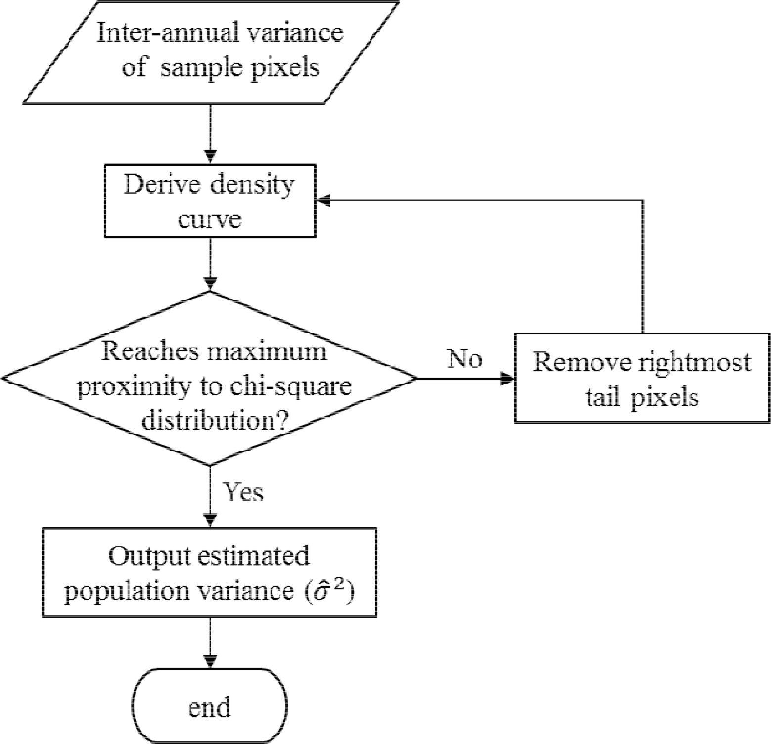
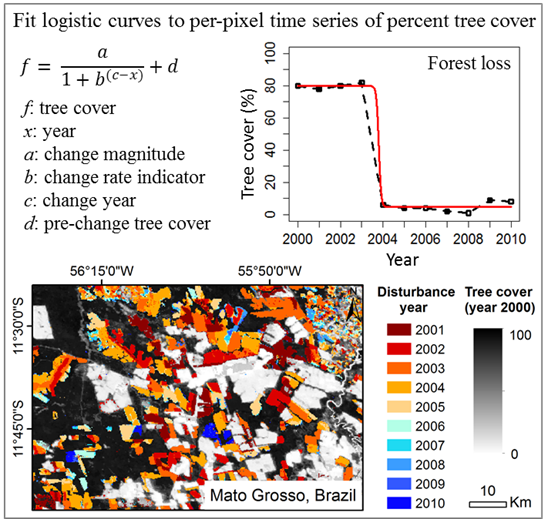
Our algorithm explicitly tracks changes in tree cover over time, as opposed to existing time series approaches of forest cover change detection (e.g., VCT [24], LandTrendr [26]), which rely on spectral indexes to infer forest cover change. This new method, which also improves upon existing empirical approaches, is developed based on the theoretical basis that land cover disturbances are rare phenomena for a relatively large area within a short time period. For example, ∼1.1% of forests in the U.S. were disturbed annually between 1985 and 2005 [18], and globally, ∼0.2% of the land surface experienced stand-clearing forest disturbances (gross forest cover loss) annually between 2000 and 2012 [20]. Repeated measures of land cover over the entire area therefore contain a majority of numerically-stable data points and a small set of outliers. Assuming that errors in the repeated measurements follow a normal distribution, well-established parametric statistical theories [57] provide proof that land cover changes are outliers of an underlying chi-square distribution. The first step of the algorithm is to separate these outliers from the majority of unchanged pixels (Figure 1). Then, for each identified change pixel, the algorithm tracks continuous changes in tree cover over time by fitting one or more nonlinear curves. Specifically, we intend to capture the sigmoid or “S” shape of forest cover change using logistic models, a close compliance with the actual physical process of land cover change on the ground. Quantitative metrics, such as the magnitude, rate and time of forest cover change in each pixel, are then derived from the parameters of the fitted logistic equations.
3.2. Identifying Candidate Change Pixels
3.2.1. Theoretical Basis
Assuming errors in the repeated estimates of tree cover are independent and identically follow a normal distribution (i.i.d.), the idea to separate changes from unchanged pixels lies in that repeated estimates over stable locations over time follow a normal distribution, while estimates over disturbed locations are outliers of the distribution. Mathematically, let x(i,t) denote the estimated percent tree cover in pixel i at time t, μ(i,t) denote the true tree cover and ε(i,t) be the associated error, then:
For any i and t, ε(i,t) is assumed to be independent and identically distributed. Following this assumption, the pixel value x(i,t) is considered as a random variable drawn from a normal distribution. For any i, the sample variance of the pixel vector over N years (x(i,1), x(i,2), ···, x(i,N)) follows a scaled chi-square distribution, with a mean of σ2 and a variance of 2σ2:
Given a sample dataset consisting of a majority of stable observations (i.e., μi constant over time) and a small proportion of outliers (i.e., μi changes), the i.i.d. normality of the dataset is violated by the inclusion of change outliers. Because change pixels typically have greater variances than those of stable pixels, stable pixels are concentrated around the peak, while change pixels are located in the tail of the distribution; the greater the variance, the more likely the pixel is an outlier (Figure 2a). Because the distribution of has a mean value of σ2 and a variance of 2σ2 for unchanged pixels, the unknown population variance (i.e., σ2) of random errors can then be estimated by the mean value of after removing change outliers.
For a dataset with a total of M pixels, let:
Compared to a standard chi-square distribution, the density curve of Y′i is supposed to have a fatter tail and a systematic shift towards the left when the sample includes outliers (Figure 2b). The objective of detecting outliers is now to search for a threshold, such that by removing likely outliers on the tail, the residual dataset has a maximum proximity to a chi-square distribution (Figure 2c).
3.2.2. Deriving Parameters of the Chi-Square Distribution
An iterative procedure was used to progressively remove the rightmost tail pixels to achieve an optimal match between the density distribution of the residual data sample and a standard chi-square distribution (Figure 3). The idea of adaptively trimming the distribution tail to approximate a theoretical chi-square distribution for outlier recognition has been applied in exploratory data analysis in many other disciplines, e.g., geochemistry [58,59]. Here, we employ the maximum likelihood estimation (MLE) framework to find the optimal threshold. The objective function in the MLE is to maximize the quantile-quantile (Q-Q) correlation coefficient (the most commonly used and effective tool for a distribution test [60]) between the residual sample and a theoretical chi-square distribution. Iteratively, the Q-Q correlation coefficient is calculated between a standard chi-square distribution and the residual sample after removing the highest variance pixel. The iteration breaks when the residual sample reaches a maximum Q-Q correlation. The mean value of this residual dataset is then an unbiased estimate of the population variance (σ̂2) of random errors (unchanged pixels).
3.2.3. Create a Change Mask Based on Probabilistic Threshold
The chi-square values corresponding to different probability levels of the simulated distribution are used as the threshold to separate likely change pixels from unchanged pixels. For example, the threshold corresponding to 0.9 probability is calculated as:
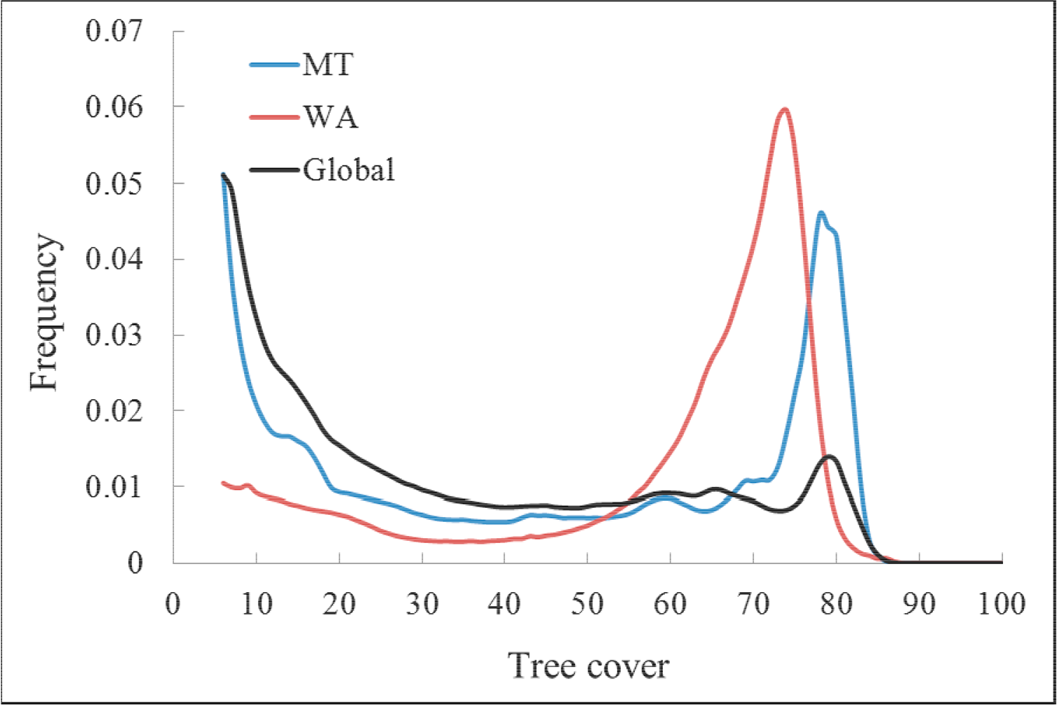
We calculated the inter-annual mean and variance of the 11-year VCF vector for each pixel and found that the strong i.i.d. assumption of the error distribution is a plausible explanation for the empirical data, but not perfectly confirmed, in part due to regional differences in measurement errors. Specifically, pixels with VCF values at the low end (0–20) and high end (60–100) tend to have relatively small variances, whereas pixels at the middle range (20–60) tend to have relatively large variances. Therefore, we stratified the dataset into a number of strata based on the inter-annual mean tree cover, subsequently applying the outlier detection on each stratum.
It should also be noted that the purpose of this outlier detection is not to detect change with 100% accuracy, but to estimate the inter-annual variance of stable pixels (σ̂2) in order to derive the probabilistic threshold and mask out the majority of unchanged pixels. We set a conservative threshold (Figure 2c) corresponding to a probability of 0.9 to capture all of the true changes without introducing significant false positives. Temporal dynamics in each pixel of this inclusive set of candidate change pixels were then modeled using logistic equations, of which the goodness-of-fit test would further discriminate true change versus false detection.
3.3. Curve Fitting to Model Change Trajectory
3.3.1. Logistic Model of Loss or Gain
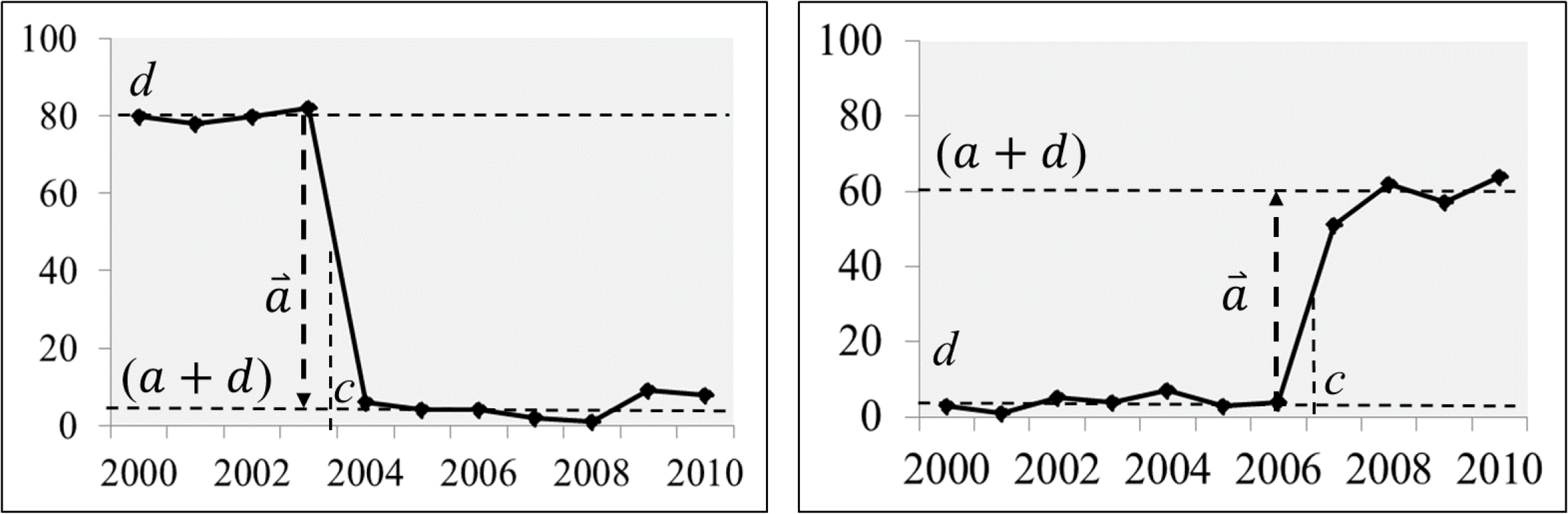
Forest cover change is reflected by the increase or decrease of the continuous tree cover values over time, which can be either abrupt (e.g., clear-cutting) or gradual (e.g., forest regrowth), and show different patterns of temporal trajectory (Figure 4). Whereas a persistent forest or non-forest pixel has a much flatter curve over time with small anomalies, a change pixel exhibits large, structural fluctuations in time series tree cover. Further, multiple successive change events could occur within the 11-year span. These structural segments are basic elements used to characterize the complete temporal trajectory for a change pixel. Capturing change events is therefore to decompose a pixel’s temporal profile into meaningful segments with distinctive structures.
Each individual change event (forest loss or gain) typically involves three distinct stages: a pre-change stage when the VCF value is stable, a change stage when the VCF value increases or declines and a post-change stage when the VCF value stays stable until the next change event occurs. This three-stage dynamic process is modeled using a logistic function:
3.3.2. Modeling Multiple Loss-Gain Processes
As multiple successive change events could occur within the 11-year span, and as the exact number of change events within the temporal profile is unknown prior to analysis, an exhaustive moving-window curve fitting is employed to capture all possible change events in the study period. Modeling multiple changes is performed in three iterations. In the first iteration, a five-year moving window is used to model a single change segment for the window focal year from 2002 to 2008. The window size of five years is chosen because (1) this ensures the minimum number of observations required to estimate four parameters and because (2) multiple forest cover changes are highly unlikely to happen within five years. It is well understood that five years may not be long enough to capture natural forest regrowth. However, since the primary objective is to detect abrupt forest loss, a shorter window size is preferred to avoid omitting forest loss signals. Goodness-of-fit for each individual curve fit is evaluated using the chi-square value of the least-squares fit. In the second iteration, the locally best fit with the smallest chi-square value is selected as the logistic model for the expected change event. Lastly, the modeled successive change events are crosschecked with each other based on a set of pre-defined neighborhood rules. For example, a clearing-cutting can be followed by an immediate plantation and, later on, by a second clearing, but cannot be followed by another immediate clearing. A maximum of two forest loss events or a maximum of two forest gain events are allowed within the 11-year period. The temporal neighborhood rules are defined such that only four specific patterns of change trajectories are detected: forest loss followed by gain, forest gain followed by loss, forest loss followed by gain and then by loss and forest gain followed by loss and then by gain (Figure 4e–h).
3.3.3. Estimating Parameters of the Logistic Model
Parameters of the logistic model are estimated as the solution to a nonlinear least-squares problem. We use MPFIT, an implementation of the iterative Levenberg–Marquardt algorithm, to perform curve fitting [62,63]. Goodness-of-fit is determined using a standard F-test (p < 0.01) based on the chi-square value of the least-squares fit. Only the statistically significant curves are saved in the final results.
4. Algorithm Evaluation
The VCA algorithm generates four output layers representing change magnitude (a), change time (c), abrupt/gradual type (b) and pre-change tree cover (d). Here, we focus our accuracy assessment on the change time layer, with an outreaching objective of evaluating the method’s performance of retrieving the disturbance area at annual resolution. Validating forest disturbance products at annual resolution remains a challenge, mainly due to a lack of reference data [14,20,24,64]. In this study, we assess the VCA disturbance map in two distinct forest biomes, where we have dense time series disturbance products derived from Landsat images as the reference. Hence, all accuracy numbers generated are relative to Landsat. We carried out the evaluation at different spatial resolutions, which is described as follows.
4.1. Deriving Reference Datasets
The first site is located in the Brazilian state of Mato Grosso within the spatial extent of MODIS tile h12v10 (hereafter referred to as the MT site). The northern part of this test area is in the tropical humid broadleaf forest biome with high-density tree canopy cover, and the southern part is in the tropical dry broadleaf forest biome with low-density canopy cover (Figure 6). This site is in the so-called “arc of deforestation” region, where large patches of primary forests were cleared for mechanized agricultural production [65]. We collected year-to-year Landsat deforestation maps derived from the PRODES (Deforestation Monitoring in the Brazilian Amazon) project by the Brazilian National Institute for Space Research (INPE, http://www.obt.inpe.br/prodes/index.php). In PRODES, Landsat data are selected at the peak of the dry season in each year to minimize cloud contamination. This reference dataset consists of 36 Landsat path/rows. The PRODES project maps deforestation in the Brazilian Amazon using Landsat images since 1988, but we only used a subset that coincides with our study period.
The second site is located in the U.S. state of Washington, near Olympic National Park (hereafter referred to as the WA site). It is within the temperate conifer forests biome with moderate to high density tree canopy cover (Figure 6). Harvesting trees for timber is the primary driver of forest cover change in this region. We collected annual growing-season Landsat images of Path 47 and Row 27 from 1984 to 2011. These Landsat images were first converted to surface reflectance through the Landsat Ecosystem Disturbance Adaptive Processing System (LEDAPS) [66] to construct a dense time series image stack [25]. This image stack was then analyzed using the vegetation change tracker (VCT) algorithm to produce an annual disturbance product [24]. The product had an overall accuracy of 93.8%, while its average user’s and producer’s accuracies for the disturbance year classes were 91.5% and 91.8%, respectively [67]. Only changes occurring between 2000 and 2010 were considered in evaluating the VCA disturbance products.
4.2. Balancing Regional Biases in Disturbance Area Estimates from MODIS
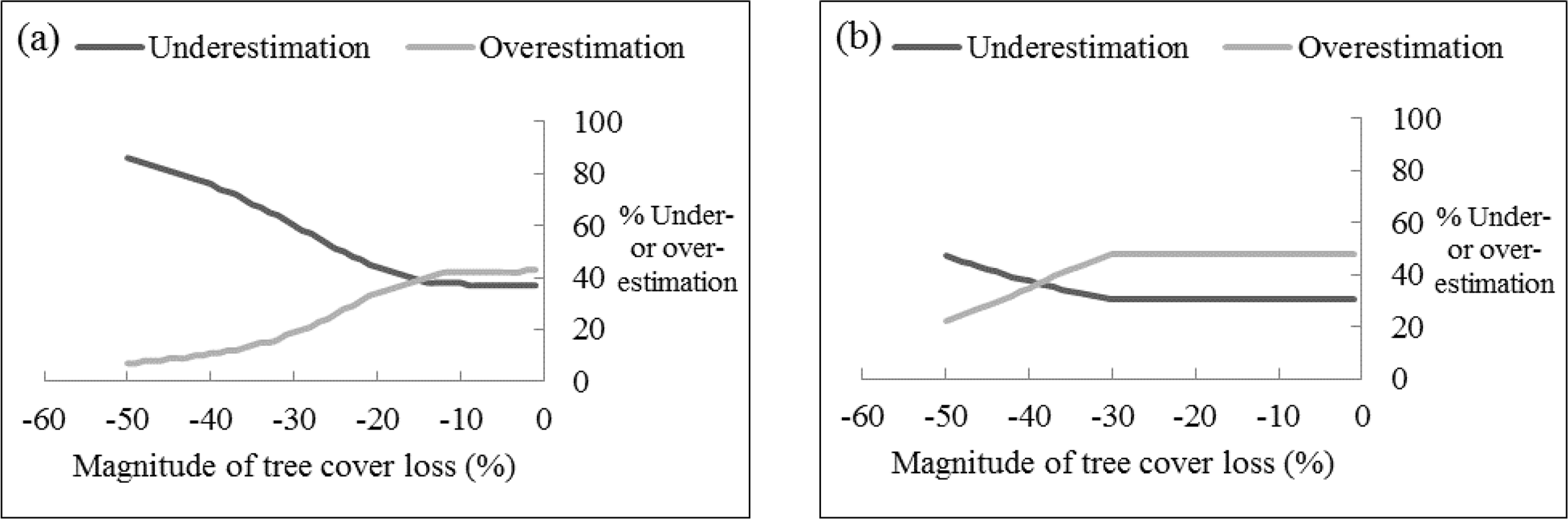
Logistic parameters (a, b, c and d) were derived for every candidate change pixel in the two test sites. Parameter a describes the magnitude of tree cover change and, therefore, is a strong indicator of forest disturbance. Obviously, varying area statistics could be generated depending on the threshold chosen to label the indicator pixels as disturbance. We first evaluated the effect of varying a as a change-detection threshold on disturbance-area estimation from MODIS against the Landsat reference. An optimal threshold was then determined, such that the overall area estimated from MODIS matched that derived from Landsat. This was achieved by balancing the deviations of the MODIS estimation from the reference, which were characterized using two metrics—underestimation and overestimation—calculated using the following equations. To do so, we resampled the MODIS pixel to 30-m resolution using the nearest neighbor resampling method with the gdalwarp function ( http://www.gdal.org).
A larger threshold (in absolute value) leads to more underestimation and less overestimation, whereas a smaller threshold leads to more overestimation and less underestimation (Figure 7). The optimal threshold that canceled out underestimation and overestimation was determined to be −39 for the MT site and −15 for the WA site. It was expected that comparing Landsat and MODIS at 30-m resolution would introduce substantial errors at the pixel scale, in part because of the differences in the original resolutions of the two sensors amplified by their different projections. MODIS pixel distortions are particularly severe in high latitudes relative to the tropics. However, the threshold searched through this comparison reaches an unbiased regional estimate of area based on MODIS, relative to the Landsat reference. The success of the change method depends in part on the availability of high-quality reference data. Although we used all of the reference data here in searching for the optimal threshold, in places where a complete reference dataset is not available, further improvement could be made to use a probability sample in a calibration procedure similar to previous studies [15,16].
4.3. Qualitative Assessment
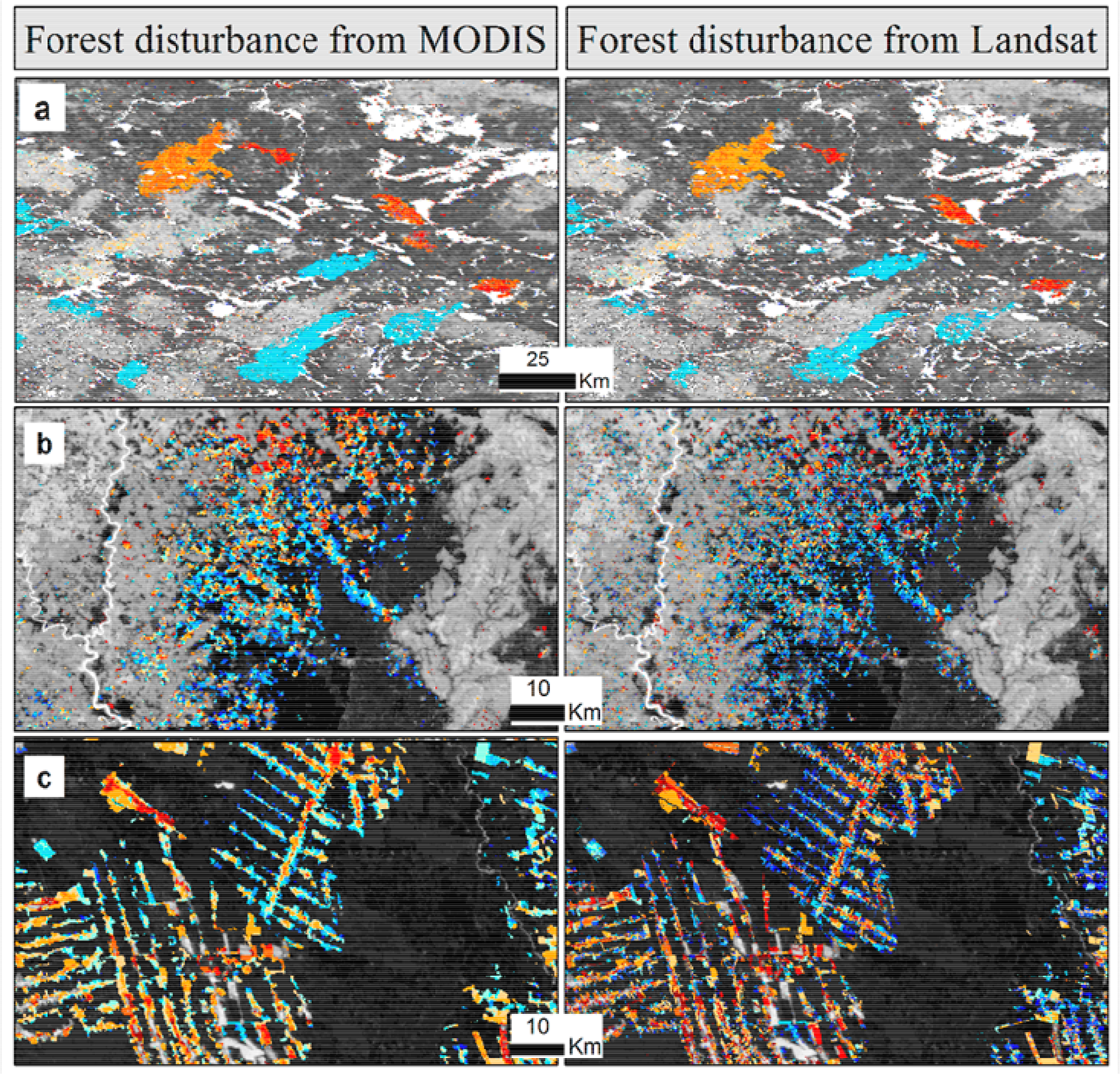
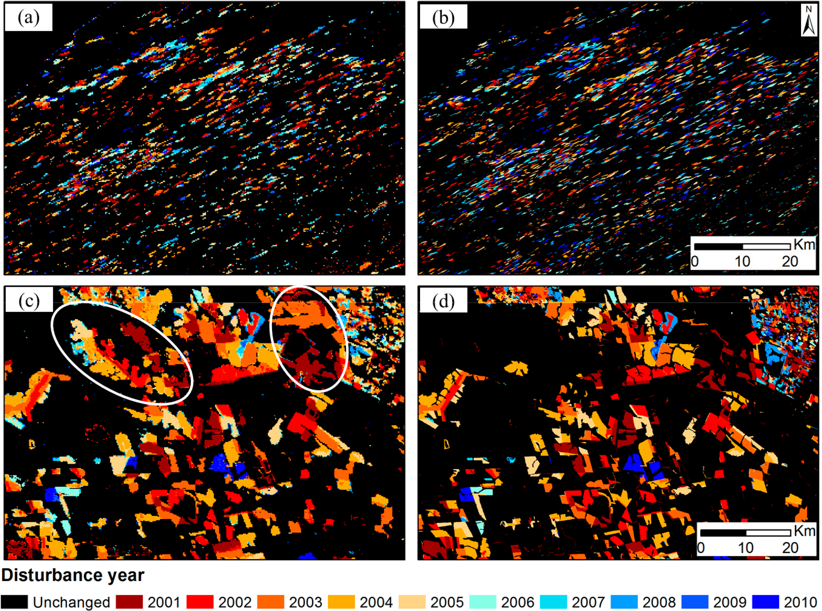
The threshold derived above was applied to obtain the final disturbance-year product from MODIS (Figure 8). Spatial and temporal patterns of disturbed land patches mapped from MODIS closely resemble those from Landsat for both test sites. The pixel-level differences observed in the Western U.S. were mainly due to the smaller size of land patches (which is comparable to a MODIS pixel), as well as the distortion of MODIS pixels at middle to high latitude. Hence, it is not surprising that smaller change patches suffer more omission and/or commission errors than relatively larger patches [68], a conclusion consistent with previous land cover change studies using MODIS data [69].
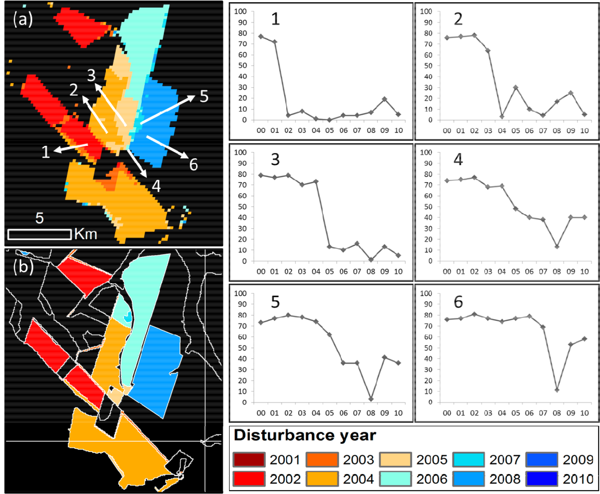
Pixel-level errors are mostly distributed on the edge of land parcels, especially when the edge is between two or more disturbed patches where the disturbances occurred in different years (see Figure 9 for an illustration). Pixels located in the middle of the patches (i.e., Pixels 1, 2, 3 and 6) show patterns of abrupt decline in tree cover in a particular year, a sign of rapid forest clearing on the ground. However, pixels located on the edge (i.e., Pixels 4 and 5) have gradual change patterns over time, which causes errors in allocating a disturbance year to the pixel. These edge pixels are either mixtures of sub-pixel disturbances occurring during different times or artifacts resulting from varying footprints of MODIS observations and the geolocation mismatch between time series MODIS layers [69–71]. Moreover, we observed that spatially adjacent patches are often disturbed in successive years in the Amazon site, whereas the clearing time for adjacent patches in the Western U.S. can be several years apart, reflecting different land management practices in these two places.
4.4. Quantitative Assessment
Applying the optimal threshold matches the 11-year total disturbance estimate from MODIS to that from Landsat at the scale of the study area. However, the accuracy of the year allocation, as well as the accuracy and precision of annual disturbance rates remain to be investigated. In this section, we first evaluate the accuracy of year allocation using a traditional error matrix at 250-m resolution and then assess the bias and precision of annual disturbance area estimates at an aggregated spatial resolution.
4.4.1. Temporal Accuracy at 250-m Resolution
To quantitatively evaluate VCA’s accuracy of determining the year of disturbance in change pixels, we applied a majority filter to the Landsat disturbance-year map, resampled it to MODIS resolution and constructed a per-pixel confusion matrix. The majority filter works as follows. Landsat pixels whose centroid falls in the MODIS grid footprint are ranked based on the frequency of their pixel value, and the most frequent value was chosen to represent the value of the aggregated grid. This was performed for each evaluation site. A strict comparison between VCA disturbance-year and the reference yielded an overall accuracy of 68.7% at the WA, USA, site and 59.8% at the MT, Brazil, site, although the accuracy for each year varied from one time to another (Tables 1 and 2). A close examination of the confusion matrices revealed that the majority of misclassifications were between neighboring years. Relaxing the allocated year to ±1 year substantially increased the accuracy for each individual year, as well as the overall accuracy. As a result, the overall accuracy achieved was 86.7% for the WA site and 84.6% for the MT site.
4.4.2. Area Accuracy at 5-km Resolution
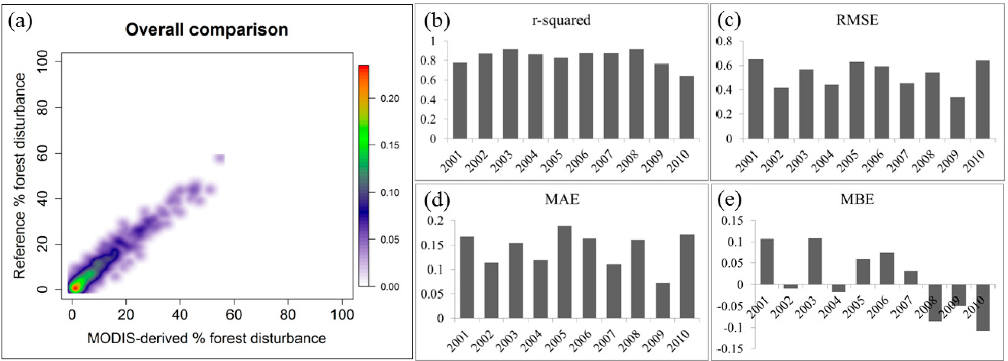
One of the practical applications of disturbance mapping is to derive the forest change rate at regional or national scales. A demonstrated way of generating such results from MODIS data is to compare and calibrate the MODIS-based estimates using temporally coincident and spatially collocated Landsat samples at a coarser resolution [15,16]. This method has been applied to quantify global forest cover loss for 2000–2005 at 20-km resolution. Here, we explore the potential of this approach in disturbance-area retrieval at an annual interval and at much finer spatial resolutions. As an example, both MODIS and Landsat disturbance products were aggregated to 5 km to calculate percent forest loss per coarse grid. We then calculated the root mean square error (RMSE), mean absolute error (MAE), mean bias error (MBE) and r2 between aggregated VCA forest loss and the reference over all 10 years, as well as for each individual year.
The comparison between VCA and Landsat at 5-km resolution in the Western U.S. had an overall r2 of 0.91 over the 10-year period. Breaking the total disturbance into individual years, the lowest r2 was in year 2010, with a value of 0.64, while all of the other years had r2 ranging between 0.77 and 0.92. The annual RMSE between VCA and Landsat disturbance ranges between 0.34% and 0.65% (Figure 10). Both high r2 and low RMSE suggest that MODIS data can be used to retrieve area estimates that approximate Landsat estimates on an annual basis. In terms of bias, the years of 2001, 2003, 2005, 2006 and 2007 had positive MBE values, indicating that MODIS overestimates forest loss in these years; conversely, the years of 2002, 2004, 2008, 2009 and 2010 had negative MBE values, indicating an underestimation by MODIS in these years. This bias pattern (i.e., overestimation in earlier years and underestimation in later years) is probably because pixels located on the edges of land patches are mislabeled and because the algorithm favors assigning an earlier year to the edge pixels (see the details in Section 4.3, Figure 9).
The comparison between VCA and PRODES in Mato Grosso yielded an overall r2 of 0.74 over the 10-year period. The annual RMSE between these two estimates ranged between 0.45% and 2.58% (Figure 11). We also found that these two products had a closer match after the year 2005, but a relatively weak relationship before the year 2005. Specifically, the VCA product identified less deforestation than PRODES in the years 2001 and 2002, but more deforestation in the years 2003 and 2004 in this region. These discrepancies were reflected in the MBE values, as well as by the scatter of observations around the 1:1 line (Figure 11a). An example of missing patches in PRODES in the years 2003 and 2004 was previously shown in Figure 8c,d, where two large deforestation patches in the upper left and upper right portion of the map were missing in PRODES. Because 36 Landsat WRS (Worldwide Reference System) tiles were used in this evaluation, cloud contamination in this Landsat dataset was unavoidable, which explained some of these omission errors in PRODES. Plus, PRODES does not capture the loss of regrowth forests on previously deforested land [23], while our VCA product detects those events successfully.
5. Discussion
The algorithm developed here provides a means to map forest disturbance at annual resolution using time series of percent tree cover estimates. The Collection 5 MODIS VCF product was used as an illustration of the algorithm. Like other time series methods for detecting change (e.g., VCT [24], BFAST (Breaks for Additive Season and Trend) [37], LandTrendr [26]), our method has the statistical advantage of increased degrees of freedom over bi-temporal change detection. A candidate change event must be confirmed by a sequence (as opposed to a pair) of observations before, during and after the change in order to be detected and identified. Moreover, although primarily designed for change detection, the idea could also be applied to remove random noise in time series of continuous field land cover product. Except for disturbance events that cause abrupt changes in tree cover, VCF values for undisturbed pixels should remain relatively stable or change gradually (e.g., resulting from natural growth) over time. Therefore, VCF values fitted to the logistic curves for those pixels likely are more realistic than the original values.
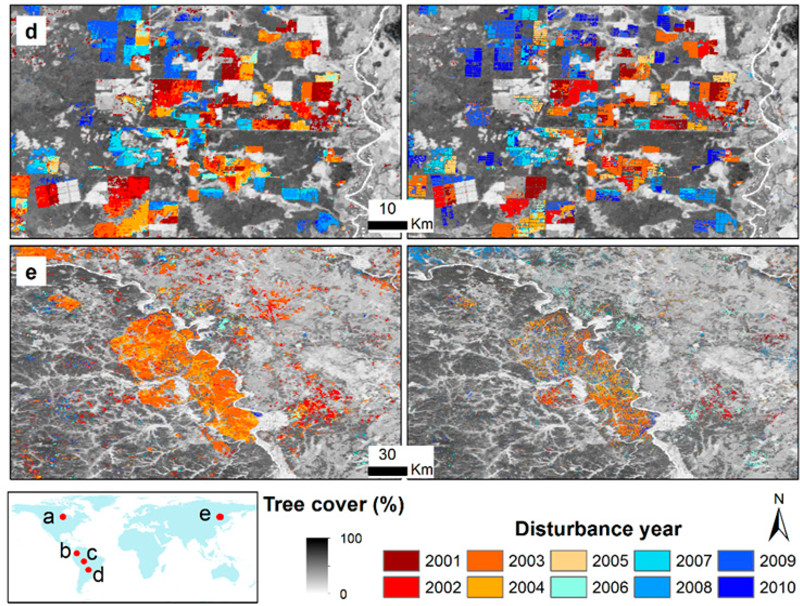
The method’s foundation in well-characterized, parametric statistical models gives it the advantage of computational simplicity. Large-area land cover mapping or change detection often requires intensive human involvement (e.g., the PRODES project) or automation, which requires either sophisticated algorithm parameterization, substantial computing facilities (e.g., [20]) or both. The method demonstrated here follows established statistical theory with little parameter fine-tuning. Although the time needed to complete a change analysis is a function of data volume, masking out the majority of stable pixels before characterizing disturbance greatly improves the method’s efficiency. As such, a global application could be completed on a single PC within a reasonable amount of time. We implemented our algorithm for application at the global scale. As a visual assessment, our initial results show great similarities with Landsat-based disturbance maps by Hansen et al. [20] in various places (Figure 12). For large disturbance patches detectable at the MODIS 250-m resolution, VCA may allow for the detection of changes missed in Landsat-based results due to the lack of clear view observations (e.g., Figure 12e). Like many other MODIS-based change studies, however, rigorous regional calibration using Landsat data is needed to derive area estimates comparable to those derived using Landsat data alone [15,16].
Another unique advantage of the method is that it characterizes continuous changes in land cover at sub-pixel resolution and has the potential to capture subtle and long-term changes, such as forest degradation. Land cover conversion often exhibits a strong contrast between remotely-sensed images at two or more time points. However, stress-induced changes within the same cover type (e.g., forest degradation) do not necessarily have apparent signatures in the short term, but may show trends over a long time span [73]. Hence, it has been suggested that to detect forest degradation, land cover should be characterized as continuous biophysical variables, and the method should be flexible to capture trends at the inter-annual scales [41,42].
This approach is not limited to tree cover, nor to the MODIS resolutions, nor to the annual time step. Although we used percent tree cover layers from MODIS as an illustration of the algorithm, the general method had no specific requirement on the thematic type or spatial or temporal resolution. Therefore, it may be applicable to continuous fields of other land cover types generated using satellite data from different sensors. Coarse-resolution sensors provide rich data at high temporal frequencies. The algorithm might be applied to the intra-annual scale to derive near real-time indicators of land cover change. At the Landsat resolution, global VCF tree cover products have been generated for 2000 and 2005 [48]. Recent advances in remote sensing demonstrated that Landsat images could be used to create near cloud-free composites by exhaustively mining the Landsat archive [20,74], and the annually composited Landsat images could also be used to characterize land cover and change [20,75]. This may create an opportunity to produce continuous fields of land cover at annual time steps using Landsat data. The approach developed here also provides the potential for such applications.
There are several limitations of the current algorithm. First, for each pixel, the sample size in the temporal domain is small (i.e., eleven data values from eleven years). The inter-annual variance calculated using eleven data samples may not well represent the actual variance of the population. A practical solution adopted here is setting conservative probabilistic thresholds for detecting change. This, however, introduces commission errors in the first step and creates redundant cases for curve fitting in the second step. Should data of longer time series be available, more precise thresholds could be located following the statistical inference and a more accurate change mask could be generated. As such, we expect the algorithm to work better as the VCF record becomes longer. Second, the i.i.d. assumption obviously simplifies the actual error structure of percent tree cover estimates. We may expect spatial correlation between different pixels and serial correlation between observations of a given pixel taken over time. The effect of spatiotemporal correlation on change detection needs to be investigated in the future. Moreover, the current algorithm is optimized for detecting single or multiple abrupt forest disturbances (e.g., clear cutting). One area of future work will be to extend the method for characterizing gradual forest changes, such as degradation or natural regrowth. One technical aspect that needs to be improved is the moving window size for detecting successive disturbances. While a fixed five-year window may be enough to capture clearing cutting and fast tree plantations, a longer window is likely needed to reliably characterize natural regrowth. An adaptive window size seems to be a useful technique to address the varying temporal length of different types of forest losses and gains. Lastly, our current algorithm evaluation only includes test sites in the tropical moist broadleaf forest biome and the temperate conifer forest biome. Given the global coverage of annual MODIS VCF and increasingly available high-resolution forest cover change datasets [18,20,31], there is no reason that the quantitative evaluation cannot be expanded to other forest/woodland biomes. Subsequently, global annual forest change estimates will be derived.
6. Conclusions
We have developed a new method, namely VCF-based change analysis (VCA), for characterizing forest disturbance using time series of satellite measurements of percent tree cover. The fact that land cover disturbances are rare events in a large geographic region leads to efficient change detection by employing well-established parametric statistics. Fitting nonlinear curves to time series, continuous estimates of tree cover simultaneously characterized the timing and intensity of forest cover change. Illustrated using the 250-m annual MODIS VCF product, the method requires little parameter fine-tuning to derive indicators of annual forest cover change and could generate accurate disturbance area estimates after calibration using data of a higher spatial resolution.
The major advantages of the new method presented here include: (1) reliable results; (2) computational simplicity; (3) global applicability; (4) flexibility to capture abrupt, as well as gradual change; and (5) capability to apply to other satellite sensors. Because increasing the frequency of forest cover change detection to annual resolution is highly desirable for understanding the global carbon cycle, further research is in progress to investigate the inter-annual variability of global forest cover change.
Acknowledgments
This study was funded by NASA’s Earth and Space Science Fellowship (NESSF) Program (NNX12AN92H), the Making Earth System Data Records for Use in Research Environments (MEaSUREs) Program (NNX08AP33A) and the Land Cover and Land Use Change Program (NNH07ZDA001N-LCLUC). Additional support was provided by NASA’s Terrestrial Ecology and Carbon Cycle Sciences Programs and the Green Fund Fellowship awarded by the University of Maryland Council on the Environment. Image processing was performed in ENVI/IDL and GDAL (Geospatial Data Abstraction Library). We thank INPE for making the PRODES deforestation data available online. We are grateful to Charlene DiMiceli and Kathrine Collins for their support of this work. We would also like to thank four anonymous reviewers, whose comments greatly improved the manuscript.
Author Contributions
Xiao-Peng Song conceived of the idea. Xiao-Peng Song, Chengquan Huang and John R. Townshend designed the experiment. Xiao-Peng Song conducted data analysis and drafted the manuscript. Xiao-Peng Song, Chengquan Huang, Joseph O. Sexton, Saurabh Channan and John R. Townshend participated in the interpretation of results and writing.
Conflicts of Interest
The authors declare no conflicts of interest.
References
- Houghton, R.A. Aboveground forest biomass and the global carbon balance. Glob. Chang. Biol 2005, 11, 945–958. [Google Scholar]
- DeFries, R.S.; Houghton, R.A.; Hansen, M.C.; Field, C.B.; Skole, D.; Townshend, J. Carbon emissions from tropical deforestation and regrowth based on satellite observations for the 1980s and 1990s. Proc. Natl. Acad. Sci. USA 2002, 99, 14256–14261. [Google Scholar]
- Achard, F.; Eva, H.D.; Mayaux, P.; Stibig, H.-J.; Belward, A. Improved estimates of net carbon emissions from land cover change in the tropics for the 1990s. Glob. Biogeochem. Cy 2004. [Google Scholar] [CrossRef]
- Houghton, R.A. Why are estimates of the terrestrial carbon balance so different? Glob. Chang. Biol 2003, 9, 500–509. [Google Scholar]
- Harris, N.L.; Brown, S.; Hagen, S.C.; Saatchi, S.S.; Petrova, S.; Salas, W.; Hansen, M.C.; Potapov, P.V.; Lotsch, A. Baseline map of carbon emissions from deforestation in tropical regions. Science 2012, 336, 1573–1576. [Google Scholar]
- Pan, Y.; Birdsey, R.A.; Fang, J.; Houghton, R.; Kauppi, P.E.; Kurz, W.A.; Phillips, O.L.; Shvidenko, A.; Lewis, S.L.; Canadell, J.G.; et al. A large and persistent carbon sink in the world’s forests. Science 2011, 333, 988–993. [Google Scholar]
- Baccini, A.; Goetz, S.J.; Walker, W.S.; Laporte, N.T.; Sun, M.; Sulla-Menashe, D.; Hackler, J.; Beck, P.S.A.; Dubayah, R.; Friedl, M.A.; et al. Estimated carbon dioxide emissions from tropical deforestation improved by carbon-density maps. Nat. Clim. Chang 2012, 2, 182–185. [Google Scholar]
- Ramankutty, N.; Gibbs, H.K.; Achard, F.; Defries, R.; Foley, J.A.; Houghton, R.A. Challenges to estimating carbon emissions from tropical deforestation. Glob. Chang. Biol 2007, 13, 51–66. [Google Scholar]
- Coppin, P.; Jonckheere, I.; Nackaerts, K.; Muys, B.; Lambin, E. Digital change detection methods in ecosystem monitoring: A review. Int. J. Remote Sens 2004, 25, 1565–1596. [Google Scholar]
- Lu, D.; Mausel, P.; Brondízio, E.; Moran, E. Change detection techniques. Int. J. Remote Sens 2004, 25, 2365–2401. [Google Scholar]
- Achard, F.; DeFries, R.; Eva, H.; Hansen, M.; Mayaux, P.; Stibig, H.J. Pan-tropical monitoring of deforestation. Environ. Res. Lett 2007. [Google Scholar] [CrossRef]
- Mayaux, P.; Pekel, J.F.; Desclee, B.; Donnay, F.; Lupi, A.; Achard, F.; Clerici, M.; Bodart, C.; Brink, A.; Nasi, R.; et al. State and evolution of the african rainforests between 1990 and 2010. Philos. Trans. R. Soc. Lond. B Biol. Sci 2013. [Google Scholar] [CrossRef]
- Huang, C.; Kim, S.; Song, K.; Townshend, J.R.G.; Davis, P.; Altstatt, A.; Rodas, O.; Yanosky, A.; Clay, R.; Tucker, C.J.; et al. Assessment of paraguay’s forest cover change using Landsat observations. Glob. Planet. Chang 2009, 67, 1–12. [Google Scholar]
- Masek, J.G.; Huang, C.; Wolfe, R.; Cohen, W.; Hall, F.; Kutler, J.; Nelson, P. North American forest disturbance mapped from a decadal Landsat record. Remote Sens. Environ 2008, 112, 2914–2926. [Google Scholar]
- Hansen, M.C.; Stehman, S.V.; Potapov, P.V. Quantification of global gross forest cover loss. Proc. Natl. Acad. Sci. USA 2010, 107, 8650–8655. [Google Scholar]
- Hansen, M.C.; Stehman, S.V.; Potapov, P.V.; Loveland, T.R.; Townshend, J.R.; DeFries, R.S.; Pittman, K.W.; Arunarwati, B.; Stolle, F.; Steininger, M.K.; et al. Humid tropical forest clearing from 2000 to 2005 quantified by using multitemporal and multiresolution remotely sensed data. Proc. Natl. Acad. Sci. USA 2008, 105, 9439–9444. [Google Scholar]
- Sexton, J.O.; Noojipady, P.; Anand, A.; Song, X.-P.; McMahon, S.; Huang, C.; Feng, M.; Channan, S.; Townshend, J.R. A model for the propagation of uncertainty from continuous estimates of tree cover to categorical forest cover and change. Remote Sens. Environ 2014. submitted. [Google Scholar]
- Masek, J.G.; Goward, S.N.; Kennedy, R.E.; Cohen, W.B.; Moisen, G.G.; Schleeweis, K.; Huang, C. United States forest disturbance trends observed using Landsat time series. Ecosystems 2013, 16, 1087–1104. [Google Scholar]
- Huang, C.; Goward, S.N.; Schleeweis, K.; Thomas, N.; Masek, J.G.; Zhu, Z. Dynamics of national forests assessed using the Landsat record: Case studies in eastern United States. Remote Sens. Environ 2009, 113, 1430–1442. [Google Scholar]
- Hansen, M.C.; Potapov, P.V.; Moore, R.; Hancher, M.; Turubanova, S.A.; Tyukavina, A.; Thau, D.; Stehman, S.V.; Goetz, S.J.; Loveland, T.R.; et al. High-resolution global maps of 21st-centry forest cover change. Science 2013, 342, 850–853. [Google Scholar]
- Jin, S.; Sader, S.A. Comparison of time series tasseled cap wetness and the normalized difference moisture index in detecting forest disturbances. Remote Sens. Environ 2005, 94, 364–372. [Google Scholar]
- Broich, M.; Hansen, M.C.; Potapov, P.; Adusei, B.; Lindquist, E.; Stehman, S.V. Time-series analysis of multi-resolution optical imagery for quantifying forest cover loss in Sumatra and Kalimantan, Indonesia. Int. J. Appl. Earth Obs. Geoinf 2011, 13, 277–291. [Google Scholar]
- Hansen, M.; Shimabukuro, Y.; Potapov, P.; Pittman, K. Comparing annual MODIS and PRODES forest cover change data for advancing monitoring of Brazilian forest cover. Remote Sens. Environ 2008, 112, 3784–3793. [Google Scholar]
- Huang, C.; Goward, S.N.; Masek, J.G.; Thomas, N.; Zhu, Z.; Vogelmann, J.E. An automated approach for reconstructing recent forest disturbance history using dense Landsat time series stacks. Remote Sens. Environ 2010, 114, 183–198. [Google Scholar]
- Huang, C.; Goward, S.N.; Masek, J.; Gao, F.; Vermote, E.; Thomas, N.; Schleeweis, K.; Kennedy, R.; Zhu, Z.; Eidenshink, J.C.; et al. Development of time series stacks of Landsat images for reconstructing forest disturbance history. Int. J. Digit. Earth 2009, 2, 195–218. [Google Scholar]
- Kennedy, R.E.; Yang, Z.; Cohen, W.B. Detecting trends in forest disturbance and recovery using yearly Landsat time series: 1. Landtrendr—Temporal segmentation algorithms. Remote Sens. Environ 2010, 114, 2897–2910. [Google Scholar]
- Kennedy, R.E.; Cohen, W.B.; Schroeder, T.A. Trajectory-based change detection for automated characterization of forest disturbance dynamics. Remote Sens. Environ 2007, 110, 370–386. [Google Scholar]
- Townshend, J.R.G.; Justice, C.O. Selecting the spatial resolution of satellite sensors required for global monitoring of land transformations. Int. J. Remote Sens 1988, 9, 187–236. [Google Scholar]
- Goward, S.; Arvidson, T.; Williams, D.; Faundeen, J.; Irons, J.; Franks, S. Historical record of Landsat global coverage: Mission operations, nslrsda, and international cooperator stations. Photogramm. Eng. Remote Sens 2006, 72, 1155–1169. [Google Scholar]
- Gutman, G.; Huang, C.; Chander, G.; Noojipady, P.; Masek, J.G. Assessment of the NASA–USGS global land survey (GLS) datasets. Remote Sens. Environ 2013, 134, 249–265. [Google Scholar]
- Townshend, J.R.; Masek, J.G.; Huang, C.; Vermote, E.F.; Gao, F.; Channan, S.; Sexton, J.O.; Feng, M.; Narasimhan, R.; Kim, D.; et al. Global characterization and monitoring of forest cover using Landsat data: Opportunities and challenges. Int. J. Digit. Earth 2012, 5, 373–397. [Google Scholar]
- Tucker, C.J.; Grant, D.M.; Dykstra, J.D. NASA’s global orthorectified Landsat data set. Photogramm. Eng. Remote Sens 2004, 70, 313–322. [Google Scholar]
- Asner, G.P. Cloud cover in Landsat observations of the Brazilian Amazon. Int. J. Remote Sens 2001, 22, 3855–3862. [Google Scholar]
- Zhu, Z.; Woodcock, C.E.; Olofsson, P. Continuous monitoring of forest disturbance using all available Landsat imagery. Remote Sens. Environ 2012, 122, 75–91. [Google Scholar]
- Kleynhans, W.; Olivier, J.C.; Wessels, K.J.; Salmon, B.P.; van den Bergh, F.; Steenkamp, K. Detecting land cover change using an extended kalman filter on MODIS NDVI time-series data. IEEE Geosci. Remote Sens. Lett 2011, 8, 507–511. [Google Scholar]
- Lunetta, R.S.; Knight, J.F.; Ediriwickrema, J.; Lyon, J.G.; Worthy, L.D. Land-cover change detection using multi-temporal MODIS NDVI data. Remote Sens. Environ 2006, 105, 142–154. [Google Scholar]
- Verbesselt, J.; Hyndman, R.; Newnham, G.; Culvenor, D. Detecting trend and seasonal changes in satellite image time series. Remote Sens. Environ 2010, 114, 106–115. [Google Scholar]
- Clark, M.L.; Aide, T.M.; Grau, H.R.; Riner, G. A scalable approach to mapping annual land cover at 250 m using MODIS time series data: A case study in the Dry Chaco ecoregion of South America. Remote Sens. Environ 2010, 114, 2816–2832. [Google Scholar]
- Healey, S.; Cohen, W.; Zhiqiang, Y.; Krankina, O. Comparison of tasseled cap-based Landsat data structures for use in forest disturbance detection. Remote Sens. Environ 2005, 97, 301–310. [Google Scholar]
- Mildrexler, D.J.; Zhao, M.; Running, S.W. Testing a MODIS global disturbance index across North America. Remote Sens. Environ 2009, 113, 2103–2117. [Google Scholar]
- Lambin, E.F. Monitoring forest degradation in tropical regions by remote sensing: Some methodological issues. Glob. Ecol. Biogeogr 1999, 8, 191–198. [Google Scholar]
- Hansen, M.C.; DeFries, R.S. Detecting long-term global forest change using continuous fields of tree-cover maps from 8-km advanced very high resolution radiometer (AVHRR) data for the years 1982–99. Ecosystems 2004, 7, 695–716. [Google Scholar]
- Annual Global Automated MODIS Vegetation Continuous Fields (MOD44B) at 250 m Spatial Resolution for Data Years Beginning Day 65, 2000–2010, Collection 5 Percent Tree Cover; University of Maryland: College Park, MD, USA, 2011. Available online: http://glcf.umd.edu/data/vcf/ (accessed on 12 September 2014).
- Lawrence, P.J.; Chase, T.N. Representing a new MODIS consistent land surface in the community land model (CLM 3.0). J. Geophys. Res.: Biogeosci 2007. [Google Scholar] [CrossRef]
- Simard, M.; Pinto, N.; Fisher, J.B.; Baccini, A. Mapping forest canopy height globally with spaceborne lidar. J. Geophys. Res.: Biogeosci 2011. [Google Scholar] [CrossRef]
- Saatchi, S.S.; Harris, N.L.; Brown, S.; Lefsky, M.; Mitchard, E.T.; Salas, W.; Zutta, B.R.; Buermann, W.; Lewis, S.L.; Hagen, S.; et al. Benchmark map of forest carbon stocks in tropical regions across three continents. Proc. Natl. Acad. Sci. USA 2011, 108, 9899–9904. [Google Scholar]
- Miles, L.; Newton, A.C.; DeFries, R.S.; Ravilious, C.; May, I.; Blyth, S.; Kapos, V.; Gordon, J.E. A global overview of the conservation status of tropical dry forests. J. Biogeogr 2006, 33, 491–505. [Google Scholar]
- Sexton, J.O.; Song, X.-P.; Feng, M.; Noojipady, P.; Anand, A.; Huang, C.; Kim, D.-H.; Collins, K.M.; Channan, S.; DiMiceli, C.; et al. Global, 30-m resolution continuous fields of tree cover: Landsat-based rescaling of modis vegetation continuous fields with Lidar-based estimates of error. Int. J. Digit. Earth 2013, 6, 427–448. [Google Scholar]
- Hansen, M.C.; DeFries, R.S.; Townshend, J.R.G.; Carroll, M.; Dimiceli, C.; Sohlberg, R.A. Global percent tree cover at a spatial resolution of 500 meters: First results of the MODIS vegetation continuous fields algorithm. Earth Interact 2003, 7, 1–15. [Google Scholar]
- Hansen, M.C.; DeFries, R.S.; Townshend, J.R.G.; Marufu, L.; Sohlberg, R. Development of a MODIS tree cover validation data set for western province, Zambia. Remote Sens. Environ 2002, 83, 320–335. [Google Scholar]
- White, M.A.; Shaw, J.D.; Ramsey, R.D. Accuracy assessment of the vegetation continuous field tree cover product using 3954 ground plots in the south-western USA. Int. J. Remote Sens 2005, 26, 2699–2704. [Google Scholar]
- Montesano, P.M.; Nelson, R.; Sun, G.; Margolis, H.; Kerber, A.; Ranson, K.J. MODIS tree cover validation for the circumpolar taiga–tundra transition zone. Remote Sens. Environ 2009, 113, 2130–2141. [Google Scholar]
- Heiskanen, J. Evaluation of global land cover data sets over the tundra–taiga transition zone in northernmost finland. Int. J. Remote Sens 2008, 29, 3727–3751. [Google Scholar]
- Song, X.-P.; Huang, C.; Sexton, J.O.; Feng, M.; Narasimhan, R.; Channan, S.; Townshend, J.R. An assessment of global forest cover maps using regional higher-resolution reference data sets. In Proceedings of the 2011 IEEE International Geoscience and Remote Sensing Symposium (IGARSS), Vancouver, BC, Canada, 24–29 July 2011; pp. 752–755.
- Schepaschenko, D.; McCallum, I.; Shvidenko, A.; Fritz, S.; Kraxner, F.; Obersteiner, M. A new hybrid land cover dataset for russia: A methodology for integrating statistics, remote sensing and in situ information. J. Land Use Sci 2011, 6, 245–259. [Google Scholar]
- Song, X.-P.; Huang, C.; Feng, M.; Sexton, J.O.; Channan, S.; Townshend, J.R. Integrating global land cover products for improved forest cover characterization: An application in North America. Int. J. Digit. Earth 2014, 7, 709–724. [Google Scholar]
- Lancaster, H.O.; Seneta, E. Chi-square distribution. In Encyclopedia of Biostatistics; John Wiley & Sons, Ltd: New York, NY, USA, 2005. [Google Scholar]
- Garrett, R.G. The chi-square plot: A tool for multivariate outlier recognition. J. Geochem. Explor 1989, 32, 319–341. [Google Scholar]
- Filzmoser, P.; Garrett, R.G.; Reimann, C. Multivariate outlier detection in exploration geochemistry. Comput. Geosci 2005, 31, 579–587. [Google Scholar]
- Garson, G.D. Testing Statistical Assumptions; Statistical Associates Publishing: Asheboro, NC, USA, 2012. [Google Scholar]
- Zhang, X.; Friedl, M.A.; Schaaf, C.B.; Strahler, A.H.; Hodges, J.C.F.; Gao, F.; Reed, B.C.; Huete, A. Monitoring vegetation phenology using MODIS. Remote Sens. Environ 2003, 84, 471–475. [Google Scholar]
- Moré, J. The levenberg-marquardt algorithm: Implementation and theory. In Numerical Analysis; Watson, G.A., Ed.; Springer Berlin Heidelberg: Berlin, Gemany, 1978; Volume 630, pp. 105–116. [Google Scholar]
- Non-Linear Least Squares Fitting in IDL with Mpfit. Available online: http://arxiv.org/pdf/0902.2850v1.pdf (accessed on 12 September 2014).
- Cohen, W.B.; Yang, Z.; Kennedy, R. Detecting trends in forest disturbance and recovery using yearly Landsat time series: 2. Timesync—tools for calibration and validation. Remote Sens. Environ 2010, 114, 2911–2924. [Google Scholar]
- Macedo, M.N.; DeFries, R.S.; Morton, D.C.; Stickler, C.M.; Galford, G.L.; Shimabukuro, Y.E. Decoupling of deforestation and soy production in the southern amazon during the late 2000s. Proc. Natl. Acad. Sci. USA 2012, 109, 1341–1346. [Google Scholar]
- Masek, J.G.; Vermote, E.F.; Saleous, N.E.; Wolfe, R.E.; Hall, F.G.; Huemmrich, K.F.; Gao, F.; Kutler, J.; Lim, T.-K. A Landsat surface reflectance dataset for North America, 1990–2000. IEEE Geosci. Remote Sens. Lett 2006, 3, 68–72. [Google Scholar]
- Huang, C.; Schleeweis, K.; Thomas, N.; Goward, S. Forest dynamics within and around the olympic national park assessed using time series Landsat observations. Remote Sensing of Protected Lands, Wang, Y., Ed.; Talyor & Francis, London, UK, 2011, 71–93. [Google Scholar]
- Lechner, A.M.; Stein, A.; Jones, S.D.; Ferwerda, J.G. Remote sensing of small and linear features: Quantifying the effects of patch size and length, grid position and detectability on land cover mapping. Remote Sens. Environ 2009, 113, 2194–2204. [Google Scholar]
- Xin, Q.; Olofsson, P.; Zhu, Z.; Tan, B.; Woodcock, C.E. Toward near real-time monitoring of forest disturbance by fusion of MODIS and Landsat data. Remote Sens. Environ 2013, 135, 234–247. [Google Scholar]
- Wolfe, R.E.; Nishihama, M.; Fleig, A.J.; Kuyper, J.A.; Roy, D.P.; Storey, J.C.; Patt, F.S. Achieving sub-pixel geolocation accuracy in support of MODIS land science. Remote Sens. Environ 2002, 83, 31–49. [Google Scholar]
- Townshend, J.R.G.; Justice, C.O.; Gurney, C.; McManus, J. The impact of misregistration on change detection. IEEE Trans. Geosci. Remote Sens 1992, 30, 1054–1060. [Google Scholar]
- Willmott, C.J. Some comments on the evaluation of model performance. B. Am. Meteorol. Sci 1982, 63, 1309–1313. [Google Scholar]
- Neigh, C.; Bolton, D.; Diabate, M.; Williams, J.; Carvalhais, N. An automated approach to map the history of forest disturbance from insect mortality and harvest with Landsat time-series data. Remote Sens 2014, 6, 2782–2808. [Google Scholar]
- Roy, D.P.; Ju, J.; Kline, K.; Scaramuzza, P.L.; Kovalskyy, V.; Hansen, M.; Loveland, T.R.; Vermote, E.; Zhang, C. Web-enabled landsat data (WELD): Landsat ETM+ composited mosaics of the conterminous United States. Remote Sens. Environ 2010, 114, 35–49. [Google Scholar]
- Hansen, M.C.; Egorov, A.; Potapov, P.V.; Stehman, S.V.; Tyukavina, A.; Turubanova, S.A.; Roy, D.P.; Goetz, S.J.; Loveland, T.R.; Ju, J.; et al. Monitoring conterminous United States (CONUS) land cover change with web-enabled landsat data (WELD). Remote Sens. Environ 2014, 140, 466–484. [Google Scholar]


| Reference Disturbance Year | ||||||||||||||
|---|---|---|---|---|---|---|---|---|---|---|---|---|---|---|
| 2001 | 2002 | 2003 | 2004 | 2005 | 2006 | 2007 | 2008 | 2009 | 2010 | Total | User’s Accuracy | User’s Accuracy (±1 year) | ||
| MODIS Disturbance Year | 2001 | 2062 | 258 | 66 | 31 | 52 | 99 | 63 | 72 | 31 | 51 | 2785 | 74.0 | 83.3 |
| 2002 | 199 | 2032 | 134 | 43 | 52 | 62 | 53 | 72 | 43 | 56 | 2746 | 74.0 | 86.1 | |
| 2003 | 91 | 633 | 2619 | 281 | 90 | 71 | 76 | 133 | 52 | 151 | 4197 | 62.4 | 84.2 | |
| 2004 | 21 | 25 | 192 | 1930 | 300 | 51 | 34 | 49 | 28 | 78 | 2708 | 71.3 | 89.4 | |
| 2005 | 40 | 31 | 80 | 422 | 2342 | 279 | 75 | 110 | 39 | 85 | 3503 | 66.9 | 86.9 | |
| 2006 | 40 | 20 | 58 | 209 | 621 | 2416 | 168 | 113 | 52 | 86 | 3783 | 63.9 | 84.7 | |
| 2007 | 28 | 12 | 18 | 35 | 123 | 453 | 1754 | 275 | 41 | 30 | 2769 | 63.3 | 89.6 | |
| 2008 | 19 | 18 | 21 | 17 | 37 | 84 | 139 | 1999 | 99 | 38 | 2471 | 80.9 | 90.5 | |
| 2009 | 12 | 9 | 8 | 9 | 11 | 18 | 15 | 293 | 877 | 127 | 1379 | 63.6 | 94.1 | |
| 2010 | 16 | 17 | 20 | 12 | 36 | 34 | 38 | 119 | 181 | 1232 | 1705 | 72.3 | 82.9 | |
| Total | 2528 | 3055 | 3216 | 2989 | 3664 | 3567 | 2415 | 3235 | 1443 | 1934 | 28,046 | |||
| Producer’s Accuracy | 81.6 | 66.5 | 81.4 | 64.6 | 63.9 | 67.7 | 72.6 | 61.8 | 60.8 | 63.7 | overall: | 68.7 | ||
| Producer’s Accuracy (±1 year) | 89.4 | 95.7 | 91.6 | 88.1 | 89.1 | 88.3 | 85.3 | 79.4 | 80.2 | 70.3 | overall: | 86.7 | ||
| Reference Disturbance Year | ||||||||||||||
|---|---|---|---|---|---|---|---|---|---|---|---|---|---|---|
| 2001 | 2002 | 2003 | 2004 | 2005 | 2006 | 2007 | 2008 | 2009 | 2010 | Total | User’s Accuracy | User’s Accuracy (±1 year) | ||
| MODIS Disturbance Year | 2001 | 29,614 | 6292 | 1662 | 758 | 662 | 179 | 126 | 158 | 36 | 37 | 39,524 | 74.9 | 90.9 |
| 2002 | 8483 | 45,350 | 7006 | 2614 | 2025 | 398 | 350 | 572 | 122 | 120 | 67,040 | 67.7 | 90.8 | |
| 2003 | 5705 | 28,727 | 82,677 | 11,611 | 6741 | 1073 | 1083 | 1782 | 355 | 313 | 140,067 | 59.0 | 87.8 | |
| 2004 | 2707 | 7286 | 18,452 | 83,728 | 17,128 | 2423 | 1883 | 2620 | 445 | 426 | 137,098 | 61.1 | 87.0 | |
| 2005 | 1199 | 3162 | 4626 | 9942 | 53,700 | 5540 | 2906 | 3674 | 550 | 341 | 85,640 | 62.7 | 80.8 | |
| 2006 | 607 | 1450 | 2014 | 2999 | 7813 | 14,062 | 4921 | 4422 | 823 | 426 | 39,537 | 35.6 | 67.8 | |
| 2007 | 352 | 683 | 779 | 1147 | 1969 | 2386 | 9485 | 4873 | 998 | 456 | 23,128 | 41.0 | 72.4 | |
| 2008 | 219 | 402 | 444 | 555 | 1080 | 561 | 1903 | 11,361 | 1406 | 749 | 18,680 | 60.8 | 78.5 | |
| 2009 | 107 | 103 | 183 | 162 | 337 | 156 | 288 | 617 | 1985 | 944 | 4882 | 40.7 | 72.6 | |
| 2010 | 50 | 50 | 69 | 54 | 88 | 26 | 39 | 78 | 96 | 2122 | 2672 | 79.4 | 83.0 | |
| Total | 49,043 | 93,505 | 117,912 | 113,570 | 91,543 | 26,804 | 22,984 | 30,157 | 6816 | 5934 | 558,268 | |||
| Producer’s Accuracy | 60.4 | 48.5 | 70.1 | 73.7 | 58.7 | 52.5 | 41.3 | 37.7 | 29.1 | 35.8 | overall: | 59.8 | ||
| Producer’s Accuracy (±1 year) | 77.7 | 86.0 | 91.7 | 92.7 | 85.9 | 82.0 | 71.0 | 55.9 | 51.2 | 51.7 | overall: | 84.6 | ||
© 2014 by the authors; licensee MDPI, Basel, Switzerland This article is an open access article distributed under the terms and conditions of the Creative Commons Attribution license (http://creativecommons.org/licenses/by/3.0/).
Share and Cite
Song, X.-P.; Huang, C.; Sexton, J.O.; Channan, S.; Townshend, J.R. Annual Detection of Forest Cover Loss Using Time Series Satellite Measurements of Percent Tree Cover. Remote Sens. 2014, 6, 8878-8903. https://doi.org/10.3390/rs6098878
Song X-P, Huang C, Sexton JO, Channan S, Townshend JR. Annual Detection of Forest Cover Loss Using Time Series Satellite Measurements of Percent Tree Cover. Remote Sensing. 2014; 6(9):8878-8903. https://doi.org/10.3390/rs6098878
Chicago/Turabian StyleSong, Xiao-Peng, Chengquan Huang, Joseph O. Sexton, Saurabh Channan, and John R. Townshend. 2014. "Annual Detection of Forest Cover Loss Using Time Series Satellite Measurements of Percent Tree Cover" Remote Sensing 6, no. 9: 8878-8903. https://doi.org/10.3390/rs6098878
APA StyleSong, X.-P., Huang, C., Sexton, J. O., Channan, S., & Townshend, J. R. (2014). Annual Detection of Forest Cover Loss Using Time Series Satellite Measurements of Percent Tree Cover. Remote Sensing, 6(9), 8878-8903. https://doi.org/10.3390/rs6098878