Comparison of Latent Heat Flux Using Aerodynamic Methods and Using the Penman–Monteith Method with Satellite-Based Surface Energy Balance

Abstract

A surface energy balance was conducted to calculate the latent heat flux (λE) using aerodynamic methods and the Penman–Monteith (PM) method. Computations were based on gridded weather and Landsat satellite reflected and thermal data. The surface energy balance facilitated a comparison of impacts of different parameterizations and assumptions, while calculating λE over large areas through the use of remote sensing. The first part of the study compares the full aerodynamic method for estimating latent heat flux against the appropriately parameterized PM method with calculation of bulk surface resistance (r_s). The second part of the study compares the appropriately parameterized PM method against the PM method, with various relaxations on parameters. This study emphasizes the use of separate aerodynamic equations (latent heat flux and sensible heat flux) against the combined Penman–Monteith equation to calculate λE when surface temperature (T_s) is much warmer than air temperature (T_a), as will occur under water stressed conditions. The study was conducted in southern Idaho for a 1000-km² area over a range of land use classes and for two Landsat satellite overpass dates. The results show discrepancies in latent heat flux (λE) values when the PM method is used with simplifications and relaxations, compared to the appropriately parameterized PM method and full aerodynamic method. Errors were particularly significant in areas of sparse vegetation where differences between T_s and T_a were high. The maximum RMSD between the correct PM method and simplified PM methods was about 56 W/m² in sparsely vegetated sagebrush desert where the same surface resistance was applied.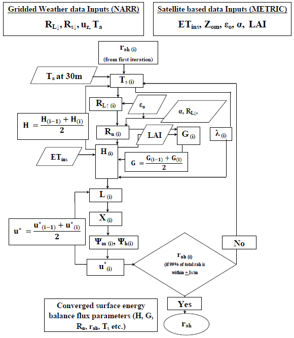

1. Introduction

The Penman–Monteith (PM) method for estimating latent heat flux (λE) calculation has long been extensively used in hydrological, atmospheric and environmental modeling. In 1948, Penman [1] combined aerodynamic bases and energy bases for calculating evaporation, which eliminating the use of the most complex meteorological parameter to be measured in the field, i.e., surface temperature. The development of satellite-based techniques has facilitated the computation of surface temperature, though data are not always available in the required temporal and spatial resolution. Mallick et al. [2] demonstrated a method that physically integrates the radiometric surface temperature into the PM equation for estimating terrestrial surface energy balance fluxes. The PM method computes relatively accurate latent heat flux (λE) in different meteorological and surface conditions when the correct parameterizations are used. However, it is commonly known to the hydrological community that the PM method can produce errors in latent heat flux calculations in sparsely vegetated areas due, in part, to: (1) the assumption of neutral atmospheric stability common to many applications for reference ET; (2) inaccurate calculation of the slope of the saturation vapor pressure curve; (3) inaccurate calculation of long-wave radiation emission from the surface; (4) underestimation of soil heat flux; and (5) mismatches between sources and sinks of momentum, heat and vapor fluxes; see, for example, Tanner and Pelton [3], Wallace et al. [4], Stannard [5], Moran et al. [6], etc. This study reinforces previous work on the difficulty in calculating λE using the PM method in sparse vegetation using satellite and weather-based data. It is essential to appropriately parameterize the PM equation when it is used to estimate λE in areas of sparse vegetation. While calculating λE using the PM method on a point scale, air temperature (T_a) is generally collected from meteorological stations at designated heights above the surface (generally ∼2–3 m). These meteorological stations generally do not record surface temperature (T_s), and many studies have based important parameters on the assumption of similarity between T_s and T_a when computing λE using the PM method. Even though T_s is not required to compute λE using the PM method, assumptions implicit to the PM can lead to error if differences between T_s and T_a are large.

Many studies conducted sensitivity analyses on parameterization and appropriate adaptation of the PM method (Thom and Oliver [7], De Bruin and Holtslag [8], Shuttleworth and Wallace [9], Allen [10], Kustas et al. [11], Moran et al. [6], Alves and Pereira [12], Gavin and Agnew [13], Nandagiri and Kovoor [14], Allen et al. [15], Gong et al. [16], Zhao et al. [17], etc.). Otles and Gutowski [18] studied atmospheric stability effects on the PM method and compared the evapotranspiration from PM to the Bowen-ratio and lysimeter data. Mukammal et al. [19] compared aerodynamic and energy balance techniques to estimate evapotranspiration from a cornfield where they discussed difficulties in using the aerodynamic method in tall crops. Results from Otles and Gutowski [18] showed that under extremely unstable boundary layer conditions, actual evapotranspiration values become smaller than estimated by the original PM formula, because under the same net input energy, the sensible heat flux is considerably larger than under neutral conditions. Thom and Oliver [7] extensively discussed the variation in estimated λE with the stability of the ratio of actual to neutral aerodynamic resistance. Allen et al. [15] discussed representative values for the bulk stomatal leaf resistance (r_l) for neutral conditions common to the so-called reference crop surfaces of alfalfa and clipped, cool season grass. Mahrt and Ek [20] discussed the influence of atmospheric stability on potential evaporation rates. Lhomme et al. [21] compared effective parameterization of the surface energy balance using various methods and conditions in heterogeneous landscape.

The main objective of this study is to emphasize the advantages of using surface energy balance via separate aerodynamic equations versus using the PM combined equations while calculating λE when surface T_s is significantly warmer than T_a. One specific objective of this study is to explore the applicability of the fully-populated PM method and the neutral boundary-layer PM method (PM_nbl) in dry and water-limited environments. These objectives were implemented through the assistance of remote sensing techniques and data.

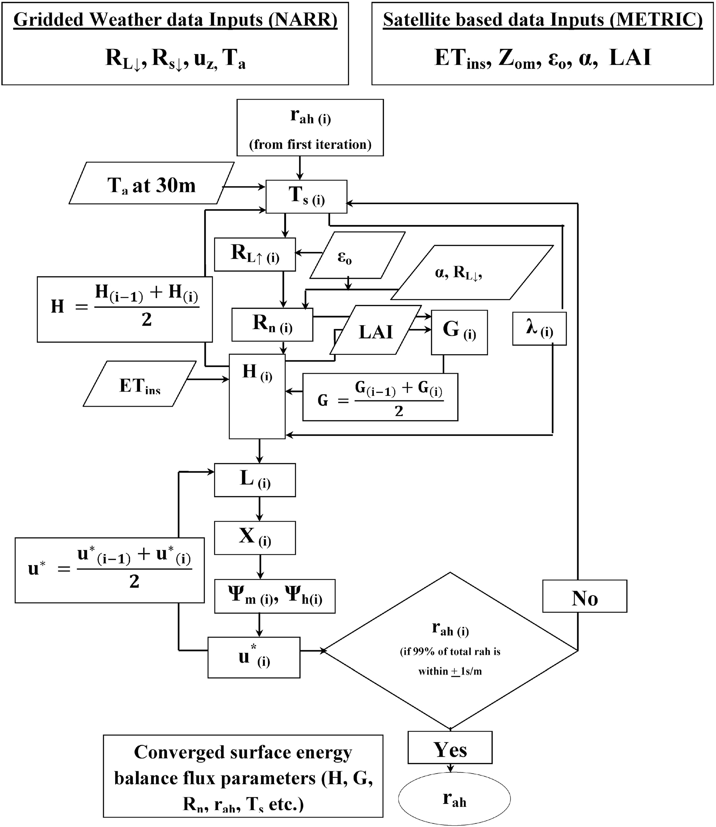
The availability of high-resolution gridded weather and remote sensing-based data has opened up important opportunities to understand and compute fluxes for different surface and atmospheric conditions. In this study, bulk surface resistance (r_s) was computed from inverting the fully-populated PM and aerodynamic (AERO) methods for latent heat flux (λE) using instantaneous ET (ET_ins) obtained from the Mapping Evapotranspiration at High Resolution using Internalized Calibration (METRIC) Landsat-image based surface energy balance. The analyses either use the same latent heat flux (λE) from the METRIC model when Landsat-based T_s is used or modifies the METRIC-generated λE based on iteratively calculated T_s. The impact of using iteratively calculated surface temperature (T_s) was examined to understand its influence on the λE calculation in both the λE_PM and λE_aero approaches. The results of the comparisons between the λE_PM and λE_aero methods show that both methods produce identical results when Δ (f = T_s, T_a)) is used in the PM method and other parameters, including net radiation (R_n), soil heat flux (G) and buoyancy, are based on full, physically-based computations. The use of the surface energy balance combined with remote sensing techniques facilitated sensitivity analysis for the computation of these fluxes, including λE. A backward-averaged accelerated numerical solution (BAANS, Dhungel et al. [22]) was used to simulate surface energy balance flux parameters based on gridded weather and satellite-based data for two satellite overpass dates under clear sky conditions, although the analysis can be extended to any atmospheric and surface condition. The description and computation procedure of the surface energy balance flux parameters using BAANS is shown in Figure 1 and detailed in Appendix A. BAANS utilizes instantaneous evapotranspiration (ET_ins) and other vegetation indices from the METRIC (Allen et al. [23]) model and gridded weather data from North American Regional Reanalysis (NARR) (Mesinger et al. [24]) (Figure 1).

The instantaneous ET estimates, ET_ins, acquired from METRIC (Allen et al. [23]) for Landsat overpass times are based on a measured radiometrically-based T_s; the latent heat of vaporization (λ) calculated in BAANS is based on an iteratively calculated T_s in order to apply the model for periods between satellite overpasses. BAANS simulates T_s iteratively inside the surface energy balance based on meteorological conditions and surface roughness by applying the Monin–Obukhov (MO) similarity theory and stability corrections. The major objective of BAANS is to estimate the surface energy flux parameters, including T_s, using a single, near-surface layer from available gridded weather sets (NARR, North American Land Data Assimilation System (NLDAS), etc.) and satellite-based roughness data (NDVI, LAI, α, ɛ_o, etc.), where the near-surface layer, at 30 m, is used as a type of “blending layer” for air temperature, specific humidity and wind speed that is extrapolated to specific surface features at the 30-m scale. This procedure gives an opportunity to compute λE over large areas when no thermal-based T_s data are available. In this study, BAANS utilizes ET_ins from the METRIC model during parameterization of surface resistances to reduce the number of iterations in the convergence process of the surface energy balance, as well as to serve as a boundary condition of latent heat flux through ET_ins. It further evaluates the accuracy of simulated T_s based on the METRIC-based ET_ins. When BAANS is implemented for non-satellite overpass times, ET_ins is computed iteratively inside the surface energy balance along with T_s. In this study, BAANS provides an opportunity to compare the surface resistance (r_s) and λE obtained from two independent and different approaches. A central question still remains regarding the accuracy of the simulated T_s from BAANS and its possible implications for the final results and conclusions. To address this, Section 4 provides an analysis based on both thermal-based T_s and simulated T_s. Both methods (AERO and PM) produced identical results, irrespective of the T_s simulated from BAANS.

2. Methodology

The procedures for calculating latent heat flux (λE) from the aerodynamic method and PM method are discussed in this section.

2.1. Aerodynamic Method of Calculating Latent Heat Flux (λE_aero)

The aerodynamic method for computing latent heat flux (λE_aero) can be expressed in a resistance form as Equation (1) (for example, Van de Griend and Owe, [25], Lhomme et al. [21], etc.).

$$\lambda {\text{E}}_{\text{aero}}=\frac{{\text{C}}_{\text{p}}{\rho }_{\text{a}}}{\gamma }\frac{({{\text{e}}^{\text{o}}}_{\text{sur}}-{\text{e}}_{\text{a}})}{({\text{r}}_{\text{ah}}+{\text{r}}_{\text{s}})}$$

(1)

where λE_aero is latent heat flux (W/m²) from the aerodynamic method, ρ_a is atmospheric density (kg/m³), C_p is the specific heat capacity of moist air (J/kg/K), e°_sur is the saturation vapor pressure of the evaporating surface (kPa), e_a is the actual vapor pressure of the air at the same height as the measured T_a (kPa), r_s is the bulk surface resistance (s/m), r_ah is the bulk aerodynamic resistance (s/m) between the surface and height of e_a and T_a measurements and γ is the psychrometric constant (kPa·°C⁻¹).

The saturation vapor pressure at the surface (e°_sur) in Equation (1) is computed using Equation (2) (Tetens [26]). In this study, surface temperature (T_s) was computed iteratively inside the surface energy balance by inverting the aerodynamic equation of sensible heat flux (H) using Equation (A2), coupled with equations for R_n, G, where H = R_n − G − λE.

$${{\text{e}}^{\text{o}}}_{\text{sur}}=0.611\text{exp}\left(\frac{17.27({\text{T}}_{\text{s}}-273.16)}{{\text{T}}_{\text{s}}-35.86}\right)$$

(2)

where T_s is in Kelvin (K). In the developed surface energy balance, outgoing longwave radiation (R_L↑) is computed from T_s using Equation (3). Most of the currently operational remote sensing-based evapotranspiration models, such as surface energy balance algorithm for land (SEBAL) (Bastiaanssen et al. [27]), METRIC (Allen et al. [23]) and Surface Energy Balance System (SEBS) (Su [28]) utilize satellite-radiatively-based T_s in the surface energy balance. In Equation (3) (BAANS), T_s is computed iteratively by inverting the aerodynamic equation of sensible heat flux (Equation (A2)).

$${\text{R}}_{\text{L}\uparrow }(\text{f}={\text{T}}_{\text{s}})={{\text{T}}_{\text{s}}}^4\sigma \hspace{0.17em}{\varepsilon }_{\text{o}}$$

(3)

where R_L↑ is outgoing longwave radiation (W/m²), ɛ_o is broadband emissivity and σ is the Stefan–Boltzmann constant (W/(m²·K⁴). In one of the comparative scenarios, the impact of using T_a to calculate R_L↑ is also investigated (Equation (4)).

$${\text{R}}_{\text{L}\uparrow \text{approx}}(\text{f}={\text{T}}_{\text{a}})={{\text{T}}_{\text{a}}}^4\sigma \hspace{0.17em}{\varepsilon }_{\text{o}}$$

(4)

where T_a is air temperature (K). Equation (4) is frequently used in hydrological applications as a relaxation of data requirements. As shown later, using T_a for outgoing longwave radiation can cause substantial error in the R_n and λE estimates for sparse and/or water-stressed vegetation. In BAANS, sensible heat flux in the surface energy balance is computed as a residual, as shown in Equation (5).

$$\text{H}={\text{R}}_{\text{n}}-\text{G}-\lambda {\text{E}}_{\text{ins}}$$

(5)

where H is sensible heat flux (W/m²), R_n is net radiation (W/m²), G is ground heat flux (W/m²) and λE_ins (separately λ ET_ins) is latent heat flux from METRIC (W/m²). R_L↑ of Equation (3) is used to compute net radiation (R_n) (Equation (6)).

$${\text{R}}_{\text{n}}=(1-\alpha ){\text{R}}_{\text{S}\downarrow }+{\text{R}}_{\text{L}\downarrow }-{\text{R}}_{\text{L}\uparrow }-(1-{\varepsilon }_{\text{o}}){\text{R}}_{\text{L}\downarrow }$$

(6)

where R_s↓ is incoming global solar radiation (W/m²), R_L↓ is downwelling longwave radiation (W/m²), R_L↑ is outgoing longwave radiation (W/m²) and α is surface albedo. Bulk surface resistance (r_{s_aero}) was computed on a 30-m pixel basis for the Landsat image domain by inverting the aerodynamic equation of latent heat flux (Equation (1)) using λE from METRIC. Shuttleworth and Wallace [9] used a similar inversion approach to compute the surface resistance at the substrate surface.

$${\text{r}}_{\text{s}\_\text{aero}}=\frac{({{\text{e}}^{\text{o}}}_{\text{sur}}-{\text{e}}_{\text{a}}){\text{C}}_{\text{p}}{\rho }_{\text{a}}}{\lambda {\text{E}}_{\text{ins}}\gamma }-{\text{r}}_{\text{ah}}$$

(7)

2.2. The Penman–Monteith Method for Calculating Latent Heat Flux (λE_PM)

The Penman–Monteith (PM) equation (Monteith [29]) for computing latent heat flux (λE_PM) is shown in its general form in Equation (8), as given, for example, by Allen et al. [30]. The PM equation, Equation (8), reverts to a suite of aerodynamic and radiation-based equations describing the full surface energy balance (including Equations (1), (3) and (A15)) when T_s is used along with T_a when calculating the slope of saturation vapor pressure curve (Δ (f = T_s, T_a)). This reversion is shown in Appendix B.

$$\lambda {\text{E}}_{\text{PM}}=\frac{\Delta ({\text{R}}_{\text{n}}-\text{G})+\frac{({{\text{e}}^{\text{o}}}_{\text{air}}-{\text{e}}_{\text{a}}){\text{C}}_{\text{p}}{\rho }_{\text{a}}}{{\text{r}}_{\text{ah}}}}{\Delta +\gamma (1+\frac{{\text{r}}_{\text{s}}}{{\text{r}}_{\text{ah}}})}$$

(8)

where Δ is the slope of the saturation pressure (kPa·°C⁻¹), R_n is the net radiation (W/m²) and G is ground heat flux (W/m²). Valiantzas [31] discussed the difficulties of calculating evapotranspiration using the PM method, largely because of the difficulties of measuring or estimating weather variables, including net radiation, vapor pressure deficit, etc. The saturation vapor pressure of air (e°_air) was computed in this study using T_a at 30 m from the NARR reanalysis data set as in Equation (9) (Tetens [26]).

$${{\text{e}}^{\text{o}}}_{\text{air}}=0.611\text{exp}\left(\frac{17.27({\text{T}}_{\text{a}}-273.16)}{{\text{T}}_{\text{a}}-35.86}\right)$$

(9)

where e°_air is in kPa.

As mentioned earlier, the ease of use and popularity of the PM method is high, since, in many applications, it does not directly depend on T_s, to calculate evapotranspiration. However, as previously discussed, applying the PM method under the PM_nbl assumptions that essentially presume a reference evapotranspiration (ET_r) condition (Allen et al. [15]; American Society of Civil Engineers—Environmental and Water Resources Institute (ASCE-EWRI) (Walter et al. [32]), where the majority of available energy is partitioned into λE, i.e., λE∼(R_n − G), so that sensible heat flux is nearly equal to zero, can lead to large errors in estimated λE for dry surfaces, due to the assumption that T_a∼T_s. It is only under conditions of a large λE rate that the assumption that T_a∼T_s is valid and the PM_nbl does not produce large errors in λE. While calculating evapotranspiration in sparse vegetation using the PM method, the calculation of Δ varies largely compared to fully-vegetated and well-watered agricultural land; this is because of the large temperature difference between surface and air in sparse vegetation. In the full PM application, the slope of saturation vapor pressure (Δ) is calculated through a linear relationship of the saturation curve between T_s and T_a (Equation (10)).

$$\Delta \hspace{0.17em}(\text{f}={\text{T}}_{\text{s}},\hspace{0.17em}{\text{T}}_{\text{a}})=\frac{{{\text{e}}^{\text{o}}}_{\text{sur}}-{{\text{e}}^{\text{o}}}_{\text{air}}}{{\text{T}}_{\text{s}}-{\text{T}}_{\text{a}}}$$

(10)

This slope of saturation vapor pressure value (Δ (f (= T_s, T_a)) is appropriate for sparse vegetation and/or drying surfaces, as it incorporates the influence of surface temperature (T_s) on the extrapolation of air temperature to the surface, implicit to the Penman combination equation derivation (Penman [1] Allen et al. [15]); however, Equation (10) requires T_s, which is generally not measured. The estimate for Δ using T_a only is shown in Equation (11), which has been widely used to calculate λE in the PM method (Allen et al. [30], Xu and Singh [33], Nandagiri and Kovoor [14], Donatelli et al. [34], etc.).

$${\Delta }_{\text{approx}}(\text{f}={\text{T}}_{\text{a}})=\frac{4098\hspace{0.17em}\left[0.6108\hspace{0.17em}\text{exp}\hspace{0.17em}\left(\frac{17.27\hspace{0.17em}{\text{T}}_{\text{a}}}{\text{T}+237.3}\right)\right]}{{({\text{T}}_{\text{a}}+237.3)}^2}$$

(11)

In this study, the impact of iteratively determining T_s was explored, where λE is calculated using the PM method with Δ from Equation (10) (Δ (f = T_s, T_a)) and from Equation (11) by Murray [35] (Δ (f = T_a)) was tested for use as an appropriate procedure. Most of the previously discussed simplifications do not account for Equation (10), while computing Δ in the PM method and using Δ_approx (f = T_a) as the appropriate procedure for calculating Δ.

Apparent values for bulk surface resistance for use in the PM equation (r_{s_PM}) were computed by inverting the PM equation (Equation (12)) using λE from METRIC. These values for r_{s_PM} are compared to r_{s_aero} (Equation (7)) below in Section 4.1 to evaluate the consistency in estimates.

$${\text{r}}_{\text{s}\_\text{PM}}=\frac{{\text{r}}_{\text{ah}}}{\gamma }\left[\frac{\Delta ({\text{R}}_{\text{n}}-\text{G})+\frac{({{\text{e}}^{\text{o}}}_{\text{air}}-{\text{e}}_{\text{a}})\hspace{0.17em}{\text{C}}_{\text{p}}{\rho }_{\text{a}}}{{\text{r}}_{\text{ah}}}}{\lambda {\text{E}}_{\text{ins}}}-(\Delta +\gamma )\right]$$

(12)

2.3. Aerodynamic Resistance (r_ah)

Aerodynamic resistance for the neutral atmospheric condition (r_{ah_neu}) was computed from Equation (13) (Thom [36], and Monteith and Unsworth [37]). The impact of using r_{ah_neu} in the PM method is discussed in one of the scenarios.

$${\text{r}}_{\text{ah}\_\text{neu}}=\frac{\text{ln}\hspace{0.17em}\left[\frac{\text{z}-\text{d}}{{\text{Z}}_{\text{om}}}\right]\text{ln}\hspace{0.17em}\left[\frac{\text{z}-\text{d}}{{\text{Z}}_{\text{oh}}}\right]}{{\text{k}}^2{\text{u}}_{\text{z}}}$$

(13)

Equation (14) is used to calculate r_ah under conditions requiring stability correction (Thom [36]).

$${\text{r}}_{\text{ah}}=\frac{\left[\text{ln}\hspace{0.17em}\left(\frac{\text{z}-\text{d}}{{\text{Z}}_{\text{om}}}\right)-{\psi }_{\text{m}}\left(\frac{\text{z}-\text{d}}{\text{L}}\right)\right]\left[\text{ln}\hspace{0.17em}\left(\frac{\text{z}-\text{d}}{{\text{Z}}_{\text{oh}}}\right)-{\psi }_{\text{h}}\left(\frac{\text{z}-\text{d}}{\text{L}}\right)\right]}{{\text{k}}^2{\text{u}}_{\text{z}}}$$

(14)

where ψ_m is a stability correction term for momentum, ψ_h is a stability correction term for heat, L is MO length (m), z is the measurement of the height of wind and temperature (m), Z_om is the roughness length of momentum (m), Z_oh is the roughness length of heat (m), u_z is wind speed (m/s), d is zero plane displacement (m) and k is the von Kármán constant, i.e., 0.41. For simplicity, the roughness length of heat transfer (Z_oh) is computed as 0.1 times Z_om for agricultural land use classes, i.e., Z_oh∼0.1 × Z_om (m). For sparse vegetation areas, like sagebrush desert and grasslands, the relationship is not kept constant. BAANS computes r_ah using Equation (13) and Δ using Equation (11) for numerical stability when differences between T_s and T_a are less than 0.01 K (near neutral atmospheric conditions).

In an ideal scenario, the λE obtained from the aerodynamic method (λE_aero) and the Penman–Monteith (λE_PM) method should be identical. For example, if identical latent heat flux (λE), aerodynamic resistance (r_ah) and surface energy flux parameters are provided for Equation (1) and Equation (8), the inverted bulk surface resistance (r_s) should be identical for both methods. Because of the various assumptions in the surface energy balance and surface roughness, as well as the closure problem in energy balance, it is not always possible to produce identical results from these methods. However, when utilizing surface energy balance, BAANS facilitated simulation of identical r_s values through the use of the same equations for aerodynamic roughness, R_n and G. Section 4.1 shows the comparison of r_s between the two models resulting in identical values from both methods.

2.4. Relaxations in the Parameterization of the Penman–Monteith Method

In this section, evaluations are carried out for the most frequently used relaxations while calculating λE using the PM method. These relaxations concern the calculation of Δ, assumptions in stability correction, the calculation procedure of R_L↑ and a combination of these.

Table 1. Parameterization of λE calculations using the Penman–Monteith (PM) method with various relaxations of important parameters and the aerodynamic method.

Condition	PM Equation for λE					Aerodynamic Equation for λE
	λE	Δ	RL↑	rah	rs	λE	RL↑	rah
λEaero	-	-	-	-	Equation (7)	Equation (1)	Equation (3)	Equation (14)
λEPM	Equation (8)	Equation (10)	Equation (3)	Equation (14)	Equation (12)	-	-	-
λEPM_Δra	Equation (8)	Equation (11)	Equation (3)	Equation (13)	Equation (12)	-	-	-
λEPM_Δ	Equation (8)	Equation (11)	Equation (3)	Equation (14)	Equation (12)	-	-	-
λEPM_ΔRL	Equation (8)	Equation (11)	Equation (4)	Equation (14)	Equation (12)	-	-	-

lists different parameterizations and assumptions that represent a combination of relaxations commonly. Table 1 also includes associated parameter equations used while calculating λE from the aerodynamic method that can change during relaxations in the PM method. λE_aero was produced by the aerodynamic method using Equation (1) with stability correction. The application of λE_aero followed the complete surface energy balance procedure outlined in Appendices A and B and in Figure 1. The results of relaxations in Table 1 are labeled (λE_{PM_Δra}, λE_{PM_Δ} and λE_{PM_ΔRL}), representing when Δ and r_a are estimated assuming neutral stability (T_s = T_a), when Δ is estimated assuming neutral stability, but r_a is estimated using iteratively estimated T_s, and when Δ, r_a and R_L↑ are estimated assuming neutral stability, respectively. The λE_{PM_ΔRL} product is commonly (and improperly) applied in practice.

The fully-parameterized PM, labeled λE_PM, is produced by the PM method using Equation (8) with stability correction, and Δ and R_L↑ are calculated with full use of iteratively derived T_s (Equation (10)). λE_PM is considered to be the correct estimate of latent heat flux from the PM method. As both λE_aero and the fully-parameterized λE_PM are calculated using converged surface energy flux parameters based on the iterative solution of T_s, they are expected to be identical, because the PM method reverts to the surface energy balance when Δ (f = T_s, T_a) (Equation (10)) is used. In the fully-populated application of the PM and aerodynamic procedures, ground heat flux (G) estimation considered the influence of T_s when T_s and T_a were different. The estimation of G was based on recent algorithms from METRIC (Allen et al. [38]).

The term “error” refers to an underestimation or overestimation of λE compared to the appropriately (i.e., fully) parameterized PM method. Both overestimation and underestimation of λE with the relaxations create problems in the closure of the surface energy balance, even if accurately measured R_n and G are used in the PM method.

In the first simplification, λE_{PM_Δra} was computed assuming a neutral atmospheric condition where stability correction factors Ψ_m and Ψ_h are assumed to be zero (Equation (13)). In this simplification, r_ah is replaced by r_{ah_neu} and Δ is replaced by Δ_approx in the PM equation, while the rest of the parameters and fluxes (i.e., R_n, G and r_s) come from the surface energy balance. λE_{PM_Δra} is computed to understand the consequences of not applying stability correction while computing λE using the PM method. This PM application includes some bias from common practice, because R_n, G and r_s may, in practice, also be affected by the simplifications in the surface energy balance, which are not accounted for.

In the second relaxation, while calculating λE_{PM_Δ} from the PM method, the slope of the saturation vapor pressure curve ((Δ) (f = T_a, T_s)) of λE_PM was replaced by Δ_approx (f = T_a), and the rest of the parameters (i.e., R_n, G, r_ah and r_s) are utilized from the fully-parameterized λE_PM. In this simplification, the consequence of using Δ_approx (f = T_a) with converged surface energy balance flux parameters and stability corrected r_ah is explored. This is one of the frequently adopted relaxations for calculating λE from the PM method; however, knowledge of surface temperature is required to estimate buoyancy correction and outgoing long-wave radiation.

In the third relaxation, while calculating λE_{PM_ΔRL}, stability correction is based on iteratively determined T_s, where the iteration is carried out for the rest of the surface energy balance flux parameters until convergence is achieved. In the λE_{PM_ΔRL} relaxation, R_n and G are based on R_L↑approx (f = T_a), and Δ is computed using Δ_approx (f = T_a). The result of this simplification is the combined effect of R_L↑approx (f = T_a) and Δ_approx. This relaxation application faces bias from common applications because λ and G are calculated based on T_s in the iteration, but the rest of the surface energy balance flux parameters are based on T_a. In this relaxation, a separate surface energy balance needs to be conducted, and the flux parameters are different than the rest of the λEs (λE_aero, λE_PM, λE_{PM_Δra} and λE_{PM_Δ}), because of the use of T_a in the surface energy balance.

The fourth relaxation is where T_s is neglected in all parameters in the surface energy balance. There was little variations in results between this and the third relaxation (λE_{PM_ΔRL}), so the discussion of this relaxation is not carried out in detail.

3. Study Area and Data

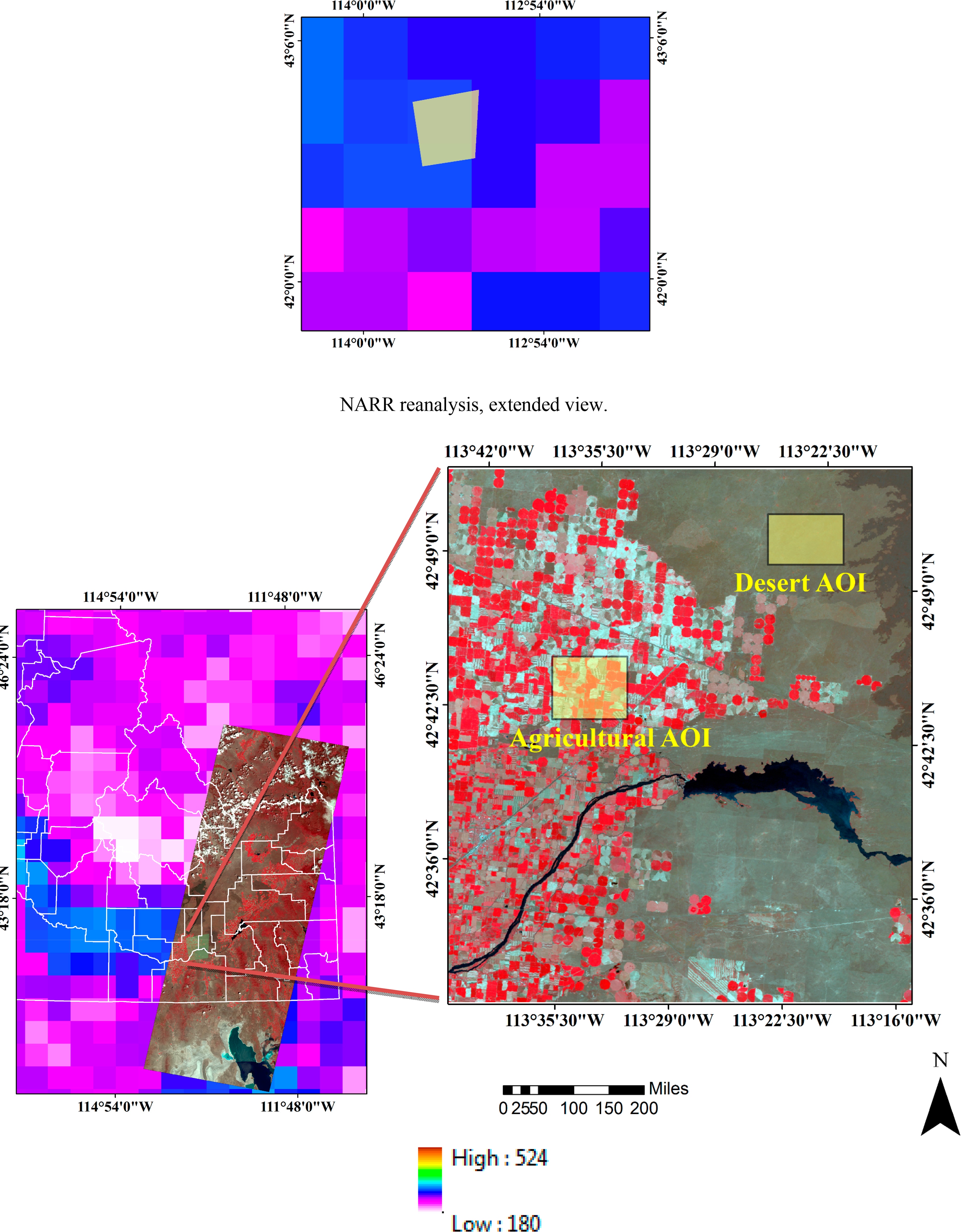
This study was conducted in a semi-arid environment in southern Idaho for a study AOI of about 1000 km², consisting of a variety of land use classes (Figure 2). The representative study area consists of about one million Landsat pixels (each one a single NARR reanalysis pixel), including irrigated agricultural, grassland, sagebrush desert areas and open water bodies. NARR reanalysis (NARR, Mesinger et al. [24]), gridded weather data and satellite-based METRIC (Allen et al. [23]) data were used to compute and close the surface energy balance. Landsat 5 images from 17 May 2008 (11:02 am), and 18 June 2008 (11:01 am), were processed using the METRIC model, where products included leaf area index (LAI), surface albedo (α), broadband emissivity (ɛ_o) and instantaneous evapotranspiration (ET_ins). There were generally crops growing during this period in agricultural parts of the image, and the application of irrigation was common. Desert soils may still have had some moisture because of winter precipitation.

A short description of the parameters used in the METRIC model is given in this section. The METRIC model computes ET_ins based on the surface energy balance as a residual of the energy balance. While calculating ET_ins, METRIC uses a water balance model to infer the impact of antecedent soil moisture on drier (and hotter) parts of the image. BAANS uses ET_ins from METRIC for calibration and initialization, so that it is impacted by the antecedent soil moisture condition. When BAANS is used for time periods in between the satellite overpass dates, a soil water balance tracks soil moisture. METRIC and the similar SEBAL model (Bastiaanssen et al. [27]) calculate reasonably accurate ET_ins, but can be impacted by the behavior of population end-members during calibration: the surface temperatures of hot and cold pixels and the available energy for the hot pixel. Although meteorological variables are necessary components of SEBAL-type models, the most critical variables that determine the performance of SEBAL/METRIC are surface temperatures and net radiation at end-members as selected by the operator. In the METRIC model, the aerodynamic function of sensible heat flux is based on the near-surface temperature difference (dT), i.e., the temperature difference between two near-surface heights. METRIC computes aerodynamic roughness Z_om based on the leaf area index (LAI) for agricultural land and uses the Perrier [39] Z_om function for tall grass and desert areas (Allen et al. [23,40]). Broadband emissivity (ɛ_o) is computed from LAI. Surface albedo (α) is calculated by integrating reflectivities from six shortwave bands of Landsat. Bastiaanssen et al. [27] and Allen et al. [23] provide details on computation of ET_ins from SEBAL and METRIC, respectively.

The central idea of this study was to utilize commonly available gridded weather data (NARR reanalysis, NLDAS, etc.) and remote sensing data to calculate λE based on the full form of the surface energy balance; a similar method has been demonstrated in Dhungel et al. [22], Dhungel and Allen [41].

Table 2. Data from NARR reanalysis for the satellite overpass date on 17 May 2008 and 18 June 2008.

NARR Data Inputs	Dates
	17 May 2008	18 June 2008
Wind speed at 30 m (uz)	1.81 m/s	4.38 m/s
Air temperature at 30 m (Ta)	297 K	296 K
Incoming shortwave radiation at surface (Rs↓)	971 W/m2	986 W/m2
Incoming longwave radiation at surface (RL↓)	310 W/m2	316 W/m2
Specific humidity at 30 m (qa)	0.0049 kg/kg	0.005 kg/kg

shows weather data from NAAR reanalysis for the two satellite dates, 17 May and 18 June 2008, for one 32-km NARR cell. Instantaneous weather data at 11:00 am from NARR reanalysis were used for the surface energy balance near satellite overpass time. NARR reanalysis data used from the 30-m height of NARR included air temperature (T_a), wind speed (u_z) and specific humidity (q_a). The 30-m height functioned as an effective blending height for extrapolating these data to surfaces of individual 30-m Landsat pixels. NARR reanalysis data for the surface included incoming shortwave radiation (R_S↓) and incoming longwave radiation (R_L↓). The incoming solar radiation (R_S↓) was relatively high at the satellite overpass times for both dates due to clear sky conditions. Those clear sky values created a large difference between the air and surface temperature for dry Landsat pixels. NARR reanalysis has a large amount of additional gridded weather data and layers other than those utilized in this study, including surface temperature, outgoing longwave radiation and outgoing shortwave radiation. However, incoming surface energy fluxes input from NARR reanalysis data have much coarser resolution than Landsat, and the variation of these meteorological parameters within the 32-km resolution pixel is assumed and precludes the use of T_s and the emitted longwave radiation at the 30-m scale, where large ranges in water availability and, thus, T_s are common. For example, localized precipitation or irrigation events, as well as surface roughness, albedo and emissivity create variation in soil moisture in the surface and root zone and, thus, outgoing energy in each Landsat pixel. As this study aimed to compute the surface energy flux parameters at the higher spatial resolution of Landsat, these variations needed to be captured using a surface energy balance at the 30-m scale. The use of the coarser resolution NARR reanalysis data to represent surface conditions and outgoing fluxes would fail to capture these variations among Landsat pixels. The question still remains whether 32-km coarse spatial resolution weather data at 30 m from NARR reanalysis can represent the incoming meteorological inputs of all approximately one million 30-m resident pixels in the surface energy balance.

To assess the impact of using large-scale weather data from NARR reanalysis, three separate analyses were conducted. In the first, NARR data from neighboring cells to the AOI were compared with that for the study AOI to evaluate spatial variation. An example is shown in Figure 2. The results suggest that the NARR reanalysis data contain negligible variation in neighboring pixels in the relatively dry Idaho climate. Secondly, NARR reanalysis data were extensively compared to various AgriMet and remote automatic weather stations (RAWS) for agricultural and desert environments, respectively, every 3 h of temporal resolution throughout the year 2008. The meteorological data compared included air temperature, wind speed, relative humidity, vapor pressure and solar radiation. Finally, theoretical clear sky radiation (R_so) from the Reference Evapotranspiration Calculator (RefET) (Allen [42]) model was compared to solar radiation from NARR reanalysis data sets. The analyses indicate that NARR reanalysis approximated actual surface meteorological measurements relatively closely.

Figure 2 shows the study area using a Landsat image from 18 June 2008, and NARR reanalysis image for the same date. The bottom left side of Figure 2 shows NARR reanalysis incoming longwave data (W/m²) for 18 June 2008, which is overlain by an Idaho county border map. The upper left figure is an expanded view of the NARR reanalysis data used in the study AOI. Incoming longwave radiation from NARR reanalysis varied between 273 and 322 W/m² in the expanded AOI with about 50 W/m² difference. Two sub-AOIs, one in agricultural land and another in sagebrush desert, were selected for statistical analysis in the 32-km study area (Figure 2).

The main objective of this paper is to emphasize the advantage of using separate aerodynamic equations versus the combined PM equation in the surface energy balance studies, when T_s is much higher than T_a. Therefore, the size of the study area and time periods of the study were constrained for this study to focus on the behavior of the methodology (e.g., Penman–Monteith), rather than on large spatial data coverage. The representative area and time periods have sufficiently explained the behaviors of the both methods. It is assumed that the meteorological data acquired from NARR reanalysis will vary little within 32-km resolution. In addition, any bias in METRIC-generated parameters and ET_ins will also be carried out in this study, but these biases do not directly influence the objectives of the study.

4. Results and Discussion

4.1. Apparent Bulk Surface Resistance (r_s)

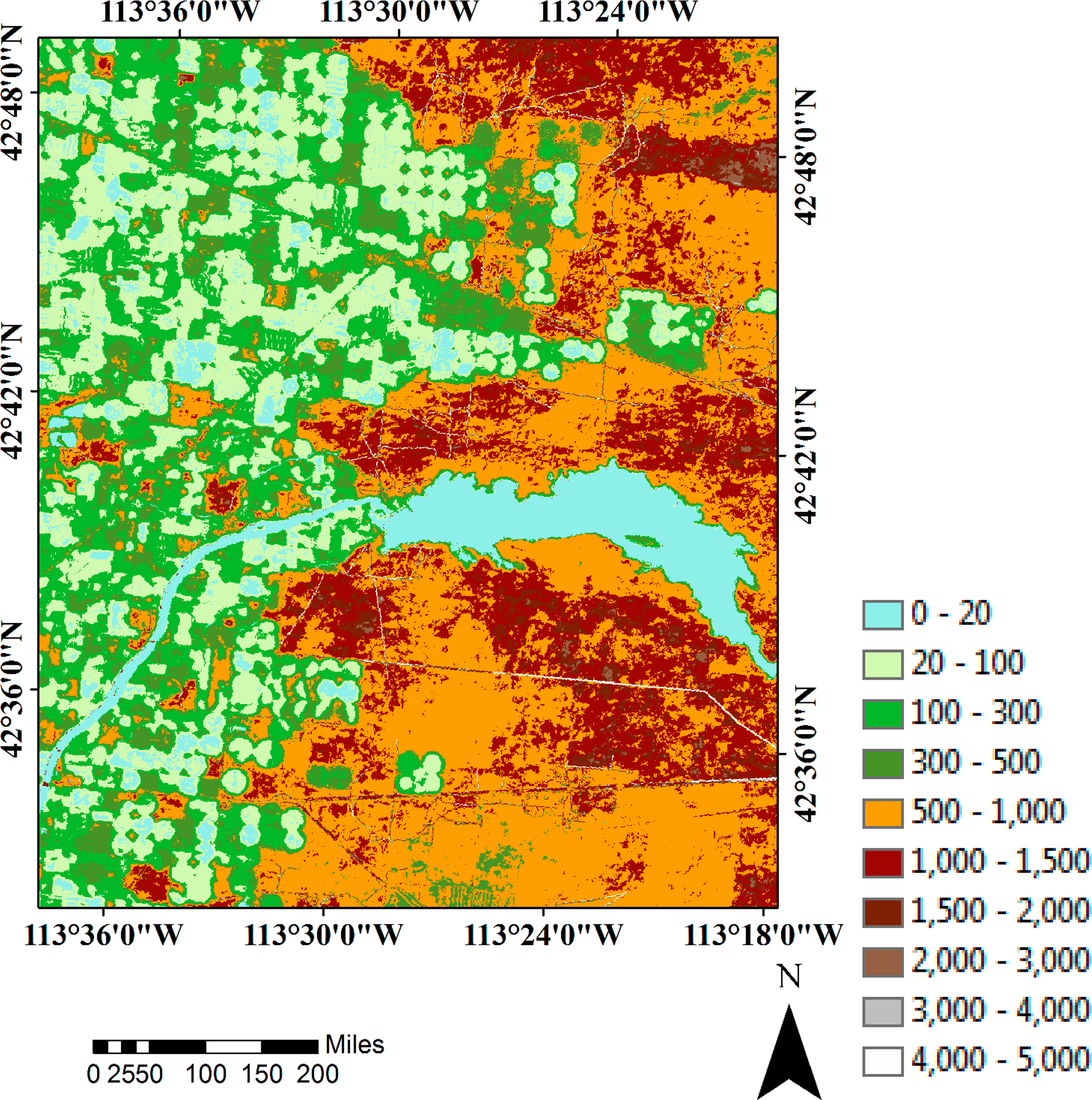
One question related to the relaxation of various environmental parameters in the PM equation is the effect of the relaxation on the value for effective bulk surface resistance (r_s) required to reproduce the same λE as produced by the full PM and full aerodynamic methods. Required values for r_s depend on the degree of relaxation, for example neglecting the effects of T_s on outgoing long-wave radiation or on Δ, or neglecting buoyancy correction. A large change in effective r_s may point to increased risk of error in estimated λE, as differences between T_s and T_a increase. In this study, apparent, effective values for r_s were computed by inverting the aerodynamic (λE_aero, Equation (7)) method and PM method (λE_PM, Equation (12)) and compared. Computations were made at Landsat over pass times using ET_ins from METRIC and simulated T_s derived through iterative calculation of the surface energy balance where λE from METRIC was an energy balance target. Satellite-based surface energy balance models, like METRIC and SEBAL, do not compute nor use r_s to calculate λE, but rather calculate λE as a residual of a thermally-driven surface energy balance. Figure 3 shows the variation in effective r_s for the study area on 18 June 2008, as determined by inverting the full PM method. Values for r_{s_PM} ranged from about 20 to 300 s·m⁻¹ for irrigated fields and from 500 to 2000 s·m⁻¹ for rangeland areas.

As discussed earlier, when the PM model is applied with outgoing longwave radiation, Δ, G and buoyancy correction, all estimated using T_s, then r_s derived from inversion of the aerodynamic and PM methods should be identical.

Table 3. Simulation results for surface energy balance flux parameters on 18 June 2008, using simulated surface temperature for all parameters in the PM.

UTM Coordinates	National Land Cover Database (NLCD) Class	ETins	LAI	α	ε	Zom	Rn	H	λE	G	Δ	ea	e°sur	e°air	Ts	rah	rs_PM	rs_aero
m	-	mm/h	-	-	-	m	W/m2	W/m2	W/m2	W/m2	kPa °C−1	kPa	kPa	kPa	K	s/m	s/m	s/m
1	2	3	4	5	6	7	8	9	10	11	12	13	14	15	16	17	18	19
5,103,099, 3,807,774	82	0.197	0.063	0.229	0.95	0.005	532	276	145	110	0.282	0.691	8.01	2.88	315	66.1	820	823
5,090,534, 3,834,428	82	0.33	0.05	0.28	0.95	0.005	500	200	219	80	0.25	0.69	6.4	2.83	311	73	388	390
5,089,869, 3,826,134	82	0.798	5.65	0.24	0.98	0.01	620	38	545	37	0.179	0.697	3.14	2.83	298	47	33	33
5,082,636, 3,817,151	82	0.63	1.26	0.157	0.96	0.022	671	131	444	96	0.207	0.698	4.3	2.83	303	56	88	88
5,085,190, 3,837,433	82	0.88	3.5	0.17	0.98	0.004	678	31	592	53	0.18	0.69	3.4	2.83	299	97	0	0
5,084,700, 3,836,226	81	0.67	0.08	0.205	0.95	0.005	617	112	412	92	0.215	0.69	4.7	2.83	305	79.4	93	93
5,101,151, 3,824,403	81	0.73	0.05	0.15	0.95	0.005	680	83	495	102	0.204	0.69	4.2	2.83	303	83	43	43
5,106,233, 3,838,590	52	0.24	0.107	0.145	0.95	0.0042	592	306	163	122	0.306	0.69	9.47	2.83	318	72	876	880
	Initial parameterizations
5,102,053, 3,814,965	52	0.17	0.043	0.148	0.95	0.3	672	397	116	159	0.216	0.696	4.73	2.83	305	22.9	599	596
	Modified parameterizations					0.045	579	331	114	133	0.318	0.696	10.16	2.83	319	71.0	1394	1400
5,100,188, 3,811,152	71	0.29	0.022	0.18	0.95	0.02	555	256	196	102	0.305	0.692	9.3	2.88	318	83	693	690
5,091,743, 3,822,013	82	0.572	2.674	0.183	0.97	0.0049	638	191	386	60	0.212	0.21	4.56	2.83	304	44	134	134

NLCD land use classes: 71, grassland; 52, sagebrush desert; 82, cultivated crops; 81, agricultural land-pasture/hay. Coordinates: Lambert conformal conic.

and

Table 4. Simulation results for surface energy balance flux parameters on 17 May 2008, using simulated surface temperature for all parameters in the PM.

UTM Coordinates	National Land Cover Database (NLCD) Class	ETins	LAI	α	ε	Zom	Rn	H	λE	G	Δ	ea	e°sur	e°air	Ts	rah	rs_PM	rs_aero
m	-	mm/h	-	-	-	m	W/m2	W/m2	W/m2	W/m2	kPa °C−1	kPa	kPa	kPa	K	s/m	s/m	s/m
1	2	3	4	5	6	7	8	9	10	11	12	13	14	15	16	17	18	19
5,103,099, 3,807,774	82	0.174	0.05	0.21	0.95	0.005	477	255	120	102	0.356	0.682	12.06	3.01	323	101	1576	1575
5,090,534, 3,834,428	82	0.14	0.007	0.26	0.95	0.005	436	243	95	98	0.34	0.685	11.27	2.93	321	103	1864	1863
5,089,869, 3,826,134	82	0.58	2.23	0.19	0.97	0.0039	603	151	387	64	0.230	0.687	5.23	2.93	307	68	140	140
5,082,636, 3,817,151	82	0.38	0.019	0.18	0.95	0.005	536	205	248	82	0.31	0.68	9.6	2.93	318	106	528	528
5,085,190, 3,837,433	82	0.33	0.05	0.21	0.95	0.005	503	202	219	81	0.31	0.68	9.57	2.93	318	107	611	611
5,084,700, 3,836,226	81	0.55	0.012	0.18	0.95	0.005	542	191	270	81	0.302	0.685	9.02	2.93	317	108	439	438
5,101,151, 3,824,403	81	0.18	0.017	0.23	0.95	0.005	466	246	120	99	0.343	0.68	11.4	2.93	322	103	1476	1476
5,106,233, 3,838,590	52	20	0.186	0.15	0.95	0.005	554	300	134	120	0.33	0.68	10.3	2.93	320	77	1207	1204
	Initial parameterizations
5,102,053, 3,814,965	52	0.16	0.071	0.154	0.95	0.3	633	376	106	151	0.234	0.687	5.42	2.93	307.4	29	761	758
	Modified parameterizations					0.061	547	315	105	126	0.33	0.687	10.76	2.93	320.4	77	1625	1621
5,100,188, 3,811,152	71	0.21	0.044	0.18	0.95	0.02	499	255	141	102	0.36	0.683	12.3	3.01	323	104	1365	1360
5,099,733, 3,826,089	82	0.68	5.11	0.234	0.98	0.0049	584	88	459	36	0.202	0.687	3.989	2.93	302	61	67	67

NLCD land use classes: 71, grassland; 52, sagebrush desert; 82, cultivated crops; 81, agricultural land-pasture/hay. Coordinates: Lambert conformal conic.

show the results of the surface energy balance for single pixels sampled from a range of land use classes at the two satellite overpass times. The computed r_s from the full PM method shows insignificant variation from that computed using the full aerodynamic method. This comparison confirms that effective r_s derived from both methods will be equal despite the accuracy of other parameters computed from BAANS if identical surface energy flux parameters are input to both methods. In the calculations, both methods utilized identical values for ρ_a, C_p, e_a, λE, γ, r_ah, R_s, R_L↓, G, T_a and e°_air. The full PM method utilized Δ from T_s (Equation (10)), whereas, the aerodynamic method used an iteratively determined e°_sur. As an example, the r_s of an agricultural pixel (5,103,099 m, 3,807,774 m) having low LAI (0.063) and with an apparently relatively dry soil surface was about 820 s·m⁻¹ when using the PM method and 823 s·m⁻¹ when using the aerodynamic method on 18 June 2008 (Table 3). The bulk surface resistance (r_s) of another agricultural pixel (5,089,869 m, 3,826,134 m) having high LAI (5.65) was about 33 s·m⁻¹ for both methods on 18 June 2008 (Table 3). That pixel had about 298 K simulated T_s, with the NARR-based air temperature ∼296 K and a sensible heat flux (H) of about 38 W·m⁻². When the ET_ins specified from METRIC was high, for example, 0.88 mm·h⁻¹ on 18 June 2008, for an agricultural pixel (5,085,190 m, 3,837,433 m) having an LAI of about 3.5, the value of r_s became very small (near zero) for both models. Of the compared pixels (Tables 3 and 4), that pixel had the smallest value for H, as the difference between T_a and T_s was small. For an agricultural pixel with low LAI (about 0.08), but an apparently wet soil surface, so that ET_ins from METRIC was about 0.67 mm·h⁻¹, the r_s was about 93 s·m⁻¹. As a comparison, Food and Agriculture Organization (FAO-56) recommends an r_s value of about 70 s/m for the well-watered grass reference evapotranspiration (ET_o) definition, based on the bulk stomatal resistance of the vegetation per unit LAI (r_l) of 100 s·m⁻¹ for 24-h calculation time steps. The r_s value will generally be smaller for hourly time steps than for daily time steps (Allen et al. [15]). Values for r_s from the inversion of the aerodynamic and full PM method are in relatively good agreement with the standardized reference r_s value.

In terms of iteratively determined T_s, BAANS simulated a lower T_s in desert and grassland areas as compared to the thermally-measured T_s from Landsat using initially-specified parameterizations for Z_om and Z_oh, while estimated T_s for agricultural land was in good agreement with Landsat-measured values (Tables 3 and 4). One of the uncertain parameters that has to be specified for the application of the surface energy balance and MO stability correction is surface roughness (Z_om, Z_oh and their interrelationships). The values for these parameters affect the aerodynamics of the energy balance (Beljaars and Viterbo [43], Mascart et al. [44], etc.) and ultimately the simulated T_s from BAANS. After modifying surface roughness values (Z_om, Z_oh and their interrelationship) in desert and grassland, BAANS was able to simulate T_s that compared better to the thermal-based T_s for sagebrush desert and grassland. With this modification, the value estimated for r_s was altered, even though both methods generated identical estimates before and after modifications to roughness (Tables 3 and 4). Table 3 shows values for r_s for land use Class 52 (sagebrush) on 18 June 2008, where LAI was 0.043 and when Z_om and Z_oh were set at initial values of 0.3 and 0.03 following Allen et al. [40]. r_s averaged about 599 s/m from both methods, with simulated T_s ∼305 K as compared to a mean T_s for the desert AOI of about 320 K. After modification of values for Z_om and Z_oh to values of 0.045 and 0.00045, r_s determined from the inversion of the PM method took on values of about 1400 s/m for both methods, with simulated T_s ∼319 K close to the measured T_s of 320 K. Tables 3 and 4 show insignificant variation in computed latent heat flux, even though the T_s varied significantly after modified parameterizations. This is because ET_ins from METRIC was specified as a boundary condition in both initial and corrected parameterizations of the surface energy balance. Other than ET_ins, the rest of the surface energy fluxes varied (i.e., R_n, G, H) based on the new simulated T_s. In this study, the final values from BAANS, after modifications, were used to compare λE computed using the relaxed parameterizations in the PM method, including the r_s derived by inverting the full PM application. A detailed discussion of the results of BAANS is presented in Dhungel et al. [22].

It is worth noting in Table 3 the differences in values for R_n that reach nearly 100 W·m⁻², even for similar albedos, due to the impact of differences in T_s on outgoing long-wave radiation. In a similar manner, values for Δ differ by up to 80% due to differences in T_s between cooler agricultural pixels and hotter rangeland pixels.

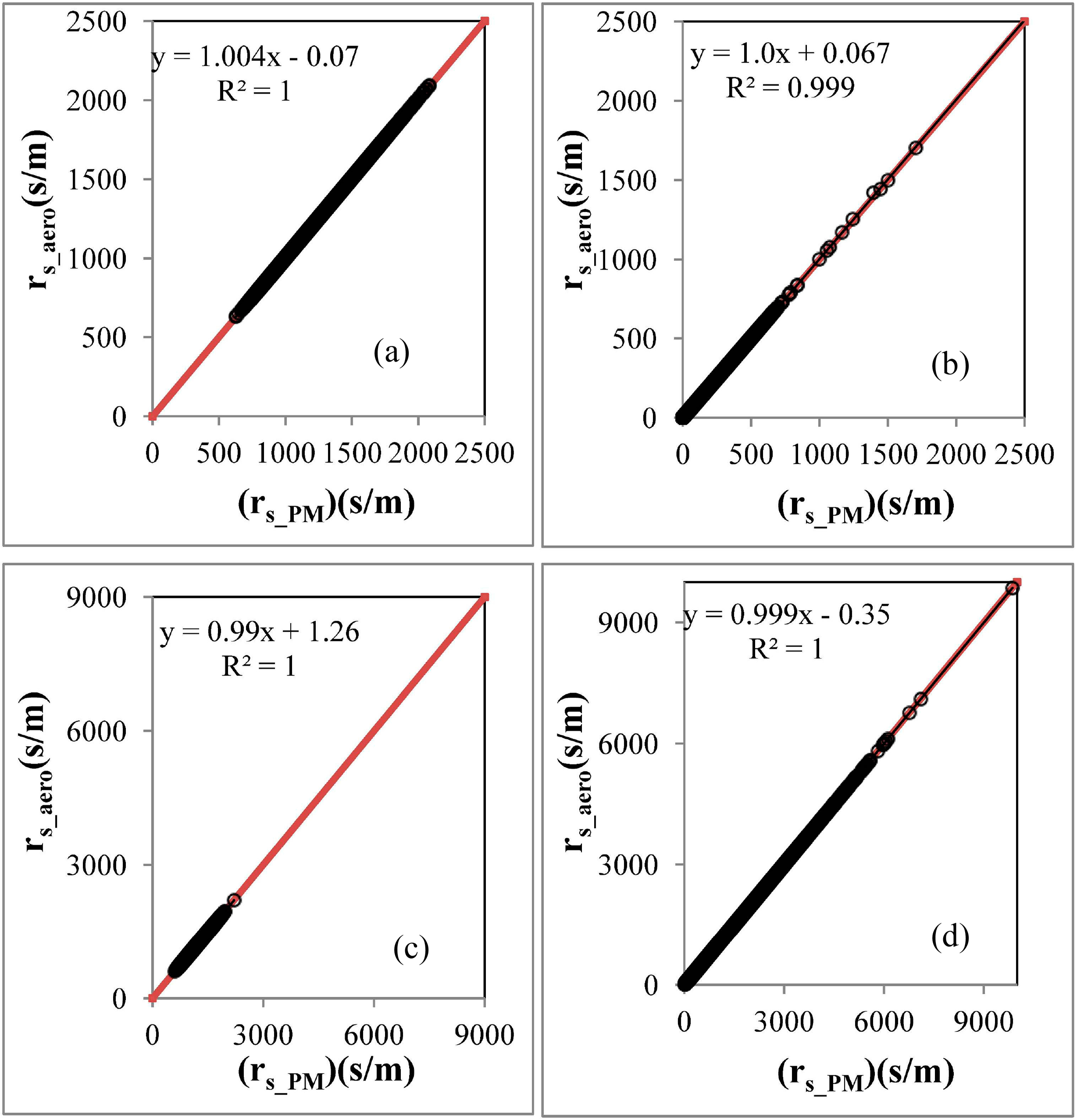
Figure 4 shows a scatter plot of r_s derived by inverting the full PM versus r_s derived by inverting the aerodynamic method for about 27,000 pixels in sagebrush desert and agricultural land AOI’s for two different dates (18 June and 17 May 2008). The results show higher values for r_s in the sparsely vegetated areas (Figure 4a), as expected, and lower values for r_s in the agricultural area, where LAI values were higher (Figure 4b). Additionally, when agricultural areas have low LAI due to bare soil conditions, r_s varies widely, exceeding the r_s of desert (Figure 4c,d). The majority of points lay on the 1:1 line, showing that both methods result in nearly identical values of r_s (Figure 4, Tables 3 and 4). The results presented in Figure 4 represent results after the modification of Z_om parameterizations in BAANS with simulated T_s.

4.2. Latent Heat Flux (λE)

Comparisons of λE are carried out in this section using the applied relaxations to the PM method to assess the impacts of Δ (f = (T_s, T_a) and Δ (f = (T_a) on ET estimates. Limited studies have made rigorous quantitative assessments of the impact of relaxations, for example Paw U [45]. A useful way to make the assessment is to cross compare estimates produced by relaxations to the PM method with calculations from the fully and properly implemented PM method or using a full surface energy balance-aerodynamic procedure, both of which are utilized in this study. Identical r_s calculated from the converged surface energy balance flux parameters (λE_areo and λE_PM, Figures 1 and 4) is used to calculate λE (λE_{PM_Δra,} λE_{PM_Δ,} λE_{PM_ΔRL}) assuming that those values for r_s represent the best and most true current values for r_s based on current atmospheric and soil water content conditions at the satellite overpass time. In this section, the comparison of λE is carried out using both simulated and Landsat-based T_s values. Thermal-based T_s from Landsat is used to verify the accuracy of simulated T_s and to explore the sensitivity of λE on error in simulated T_s. The results from Section 4.1 confirmed that a robust and workable parameterization is obtained from the full PM method, where T_s is used to calculate outgoing longwave radiation, the slope of the saturation vapor pressure curve, the soil heat flux and the boundary layer stability. Estimates by the full PM application are denoted as λE_PM. The primary surface energy balance fluxes of this study are driven by NARR reanalysis gridded weather data using vegetation indices from the METRIC model (Section 4.1). This process utilizes ET_ins from METRIC in the surface energy balance to assess values for r_s determined by inversion of the PM model when applied with various relaxations. Figure 5 shows the λE_PM based on the simulated T_s for 17 May and 18 June 2008, which is used to compare to results of relaxations to the PM over an extended area that covers both agricultural and desert AOIs.

4.2.1. Impacts of Using Δ_approx and the Assumption of Neutral Conditions (ψ_m = 0, ψ_h = 0) (λE_{PM_Δra})

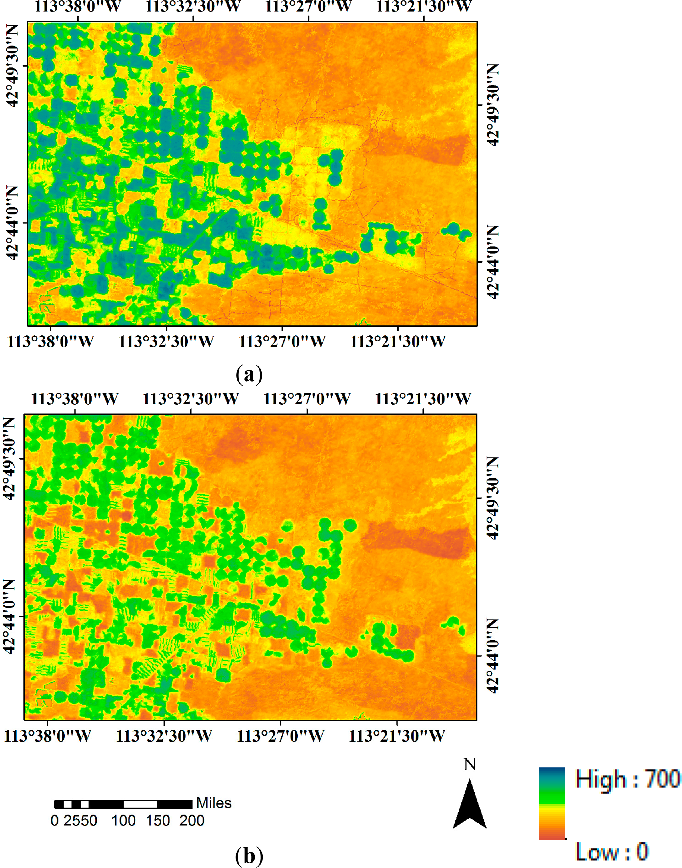
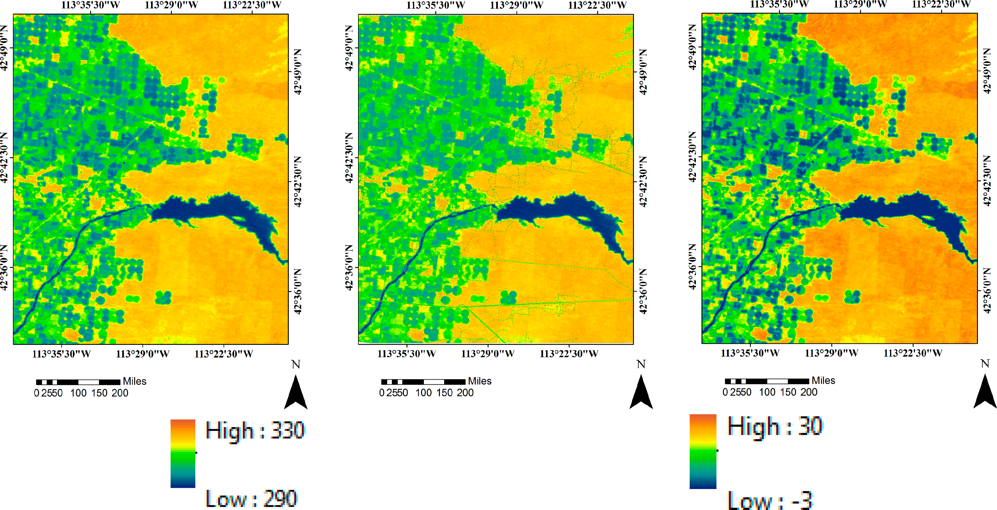
The use of Δ_approx and the assumption of neutral atmospheric conditions are commonly practiced simplifications or relaxations when computing λE from the PM method; see, for example, Lankreijer et al. [46], Penman [1], etc. Figure 6 shows Landsat-based T_s, simulated T_s from BAANS and differences between Landsat-based T_s and NARR-based air temperature, T_a, respectively, on 18 June 2008. Simulated T_s from BAANS followed Landsat-based T_s relatively closely for all land use classes (Figure 6b). Figure 6c shows differences between Landsat-based T_s and T_a that was very large, up to 30 K, in desert and grassland areas, as well as in the sparsely vegetated agricultural land. NARR-based T_a at 30 m was about 296 K at the Landsat overpass time on 18 June 2008.

The neutral stability condition basically assumes sensible heat flux (H) to be zero, partitioning the available energy into latent heat flux (λE). In a neutral atmospheric condition, aerodynamic resistance (r_{ah_neu}) is larger than the stability-corrected r_ah in an unstable condition. Lower u_z and smaller Z_om values also increase the value of r_ah for a neutral atmospheric condition. The slope of saturation vapor pressure (Δ (f = (T_s, T_a)) is equal to Δ_approx (f = T_a) for the neutral atmospheric condition, because T_s and T_a, by definition, are nearly identical. The slope of saturation vapor pressure (Δ_approx (f = T_a)) is smaller than Δ (f = (T_s, T_a) for the unstable condition where values for T_s are greater than for T_a. The slope of saturation vapor pressure (Δ) exponentially increases with increasing T_s in Equation (10) (Monteith [29]), while Δ in Equation (11) remains constant based on T_a. As both r_ah and Δ are in the numerator and denominator of the PM equation, the impact of these relaxations (larger value for r_ah for the assumed neutral atmospheric condition and smaller value for Δ using T_a only) is somewhat moderated in the PM method. However, the impacts can still be large.

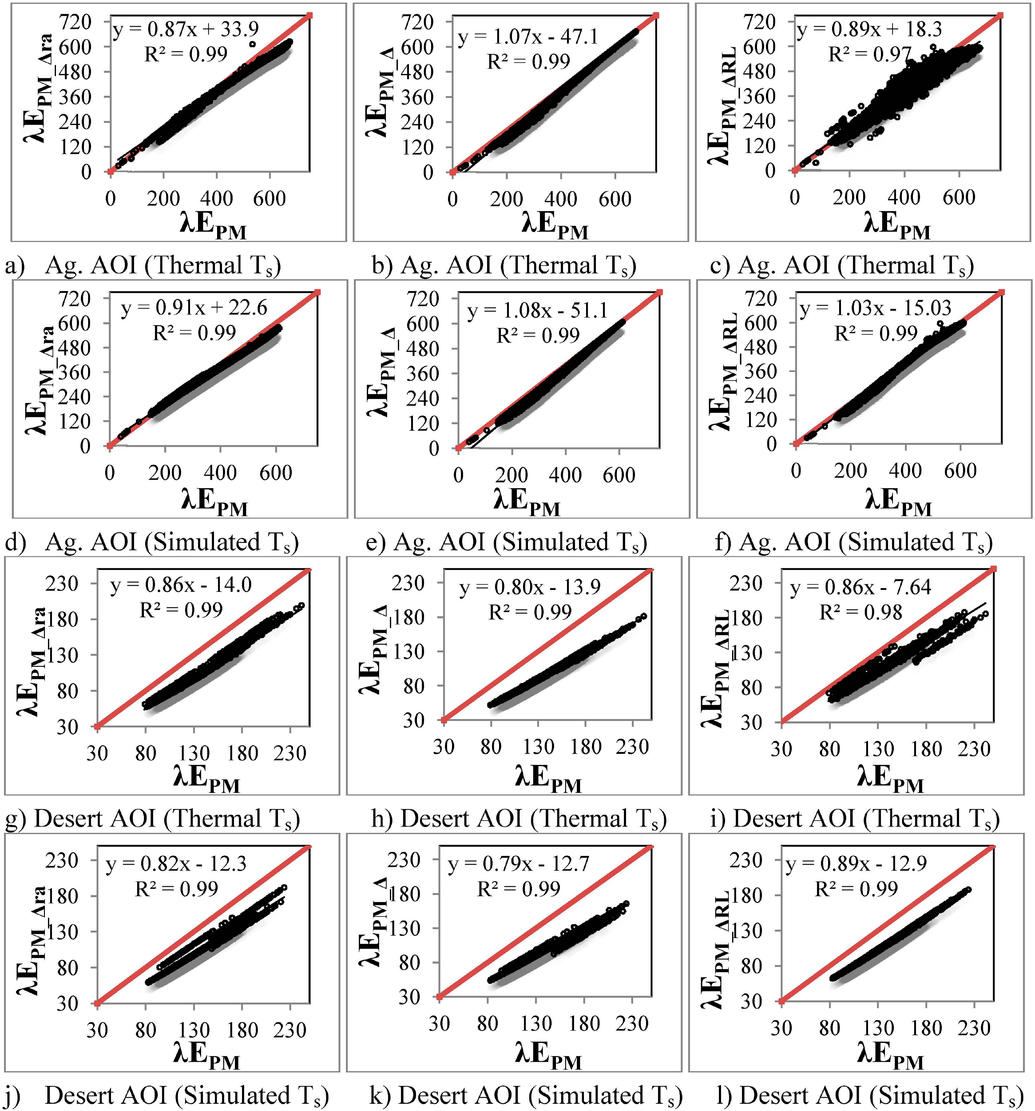
Figure 7a–c shows scatter plots for three estimates for λE based on different combinations of relaxations (simplifications) of the PM equation versus full application of the PM using Landsat-based T_s. Figure 7d–f shows the results for the same relaxations, but based on the simulated T_s produced in BAANS. Results were sampled from an agricultural AOI for 18 June 2008. Similarly, Figure 7g–i shows the results for Landsat-based T_s, and Figure 7j–l shows the results for simulated T_s for the desert AOI on the same date. NARR-based air temperature (T_a) at the 30-m blending height was about 296 K, while simulated T_s varied from 295 to 330 K for different land use classes, except water bodies (Figure 6). As discussed earlier, BAANS was able to simulate the relatively lower values for T_s in fully covered agricultural land and the higher values in sagebrush desert and grassland areas relatively well, producing values similar to Landsat-based T_s (Figure 6a,b). Figure 7 shows that application of the fully-parameterized PM method using simulated T_s produced nearly identical trends in λE as compared with those estimated based on Landsat T_s in both agricultural and desert AOIs.

The scatter plots of λE in the agricultural AOI (Figure 7a,d) show good agreement in λE produced by relaxations of the PM method and the fully-parameterized PM, due to the similarity between T_s and T_a for many of the irrigated fields, while in the sagebrush desert AOI, λE was systematically underestimated by the relaxations (Figure 7g,j). The root-mean-square deviation (RMSD) between λE_{PM_Δra} and λE_PM for the Landsat overpass time on 18 June 2008, was about 25.6 W/m² and 18.5 W/m² for the agricultural AOI using Landsat-based and simulated T_s, respectively, using λE_PM as the basis. Similarly, for the desert AOI, RMSD was about 32.4 W/m² and 32.1 W/m² from Landsat-based and simulated T_s, respectively. The coefficient of determination (R²) was 0.99 for all four scenarios (Figure 7a,d,g,j), indicating strong correlation among estimates, but with strong biases (error) for some of the relaxations.

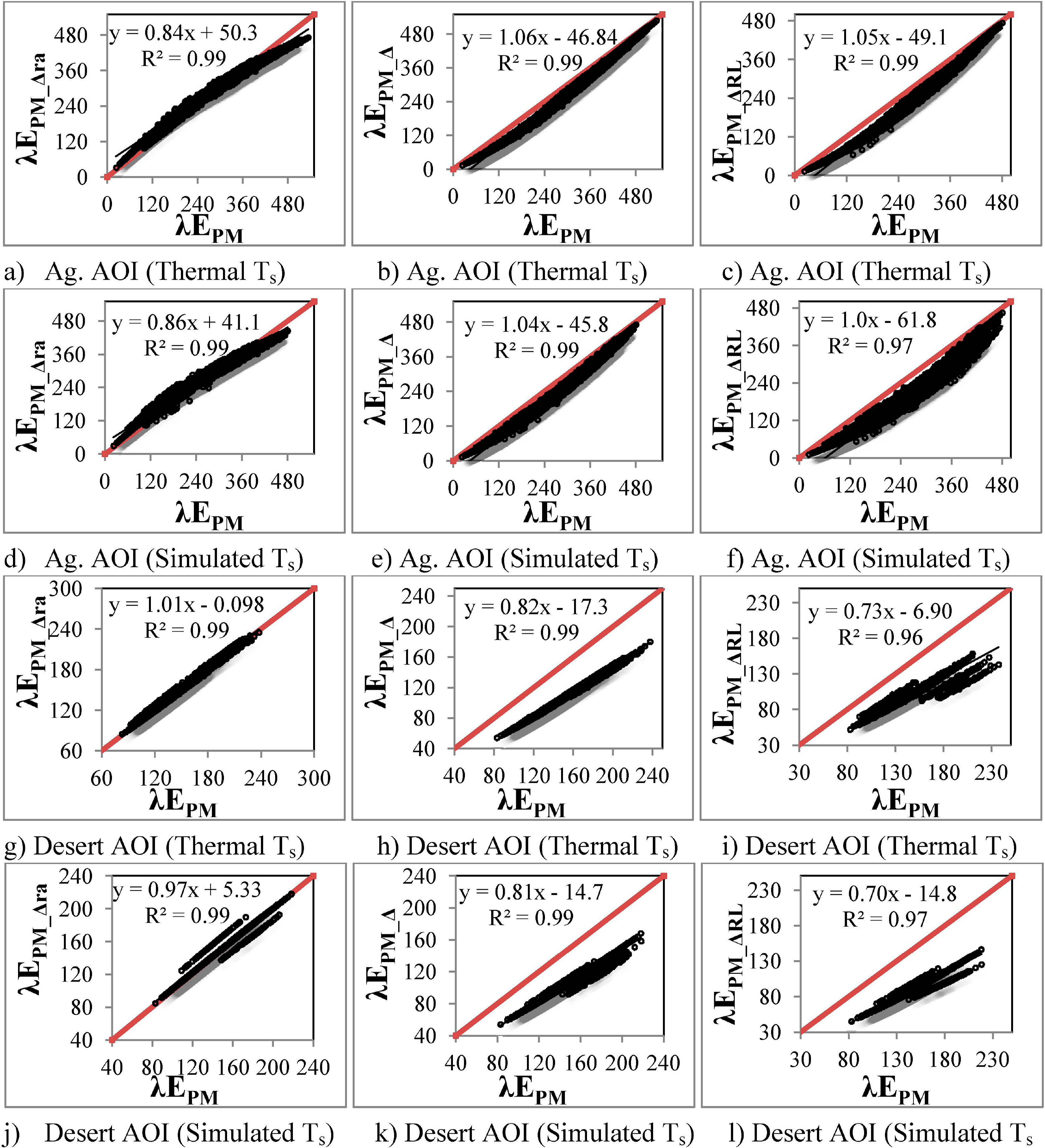
Figure 8a,d,g,j presents similar information as for Figure 7, but for the Landsat overpass time on 17 May 2008. Figure 8a,d shows that the impact of the λE_{PM_Δra} relaxation on 17 May 2008, when wind speed was smaller (1.8 m/s) than on 18 June 2008 (4.4 m/s), was to increase estimates for λE slightly in lower λE areas (having sparse or stressed vegetation) and to slightly decrease λE in higher λE areas in the agricultural AOI. Apart from the reduced wind speed, Z_om values were generally smaller for agricultural lands on 17 May, as compared to 18 June, because of being earlier in the growing season. Similarly, λE estimates for the sagebrush desert AOI were less impacted by the relaxations on 17 May 2008 (Figure 8g,j), than for the June date. This is probably because of some moderating effects caused by the combination of assumed neutral aerodynamic resistance (rah_{_neu}), lower wind speed (u_z) and neutral Δ_approx. The RMSD between λE_{PM_Δra} and λE_PM was 23.4 W/m² and 17.5 W/m² using Landsat-based and simulated T_s, respectively, for the agricultural AOI on 17 May 2008. Similarly, for the desert AOI, RMSD was 1.62 W/m² and 2.6 W/m² for Landsat-based and simulated T_s, respectively, for the same date. The coefficient of determination (R²) is 0.99 for all four scenarios (Figure 8a,d,g,j) on 17 May 2008.

Table 5. Summary of simulation results for estimated latent heat flux (λE) and percentage change relative to the full aerodynamic and PM applications (λE_aero and λE_PM), based on simulated surface temperature on the 18 June 2008 and 17 May 2008, Landsat overpass date.

Coordinates	NLCD Class	λEaero	λEPM	λEPM_Δra	Change	λEPM_Δ	Change	λEPM_ΔRL	Change
m		W/m2	W/m2	W/m2	Percent	W/m2	Percent	W/m2	Percent
1	2	3	4	5	6	7	8	9	10
18 June 2008
5,103,099, 3,807,774	82	145.9	145.5	147.8	1.5	113.5	−22.0	126.0	−13.4
5,090,534, 3,834,428	82	219.5	219.1	220.6	0.7	189.2	−13.6	206.3	−5.8
5,089,869, 3,826,134	82	544.8	544.9	521.2	−4.4	543.8	−0.2	552.6	1.4
5,082,636, 3,817,151	82	444.0	443.8	429.2	−3.3	429.0	−3.3	448.3	1.0
5,085,190, 3,837,433	82	592.5	592.5	555.4	−6.3	590.4	−0.4	610.7	3.1
5,084,700, 3,836,226	81	412.3	412.1	394.1	−4.4	395.2	−4.1	420.4	2.0
5,101,151, 3,824403	81	495.0	494.9	466.7	−5.7	484.1	−2.2	508.5	2.8
5,106,233, 3,838,590	52	163.0	163.3	127.1	−22.2	118.6	−27.4	134.0	−18.0
5,102,053, 3,814,965	52	113.5	113.7	84.9	−25.3	78.0	−31.4	89.1	−21.6
5,100,188, 3,811,152	71	195.7	195.9	169.7	−13.4	148.3	−24.3	168.3	−14.1
5,088,604, 3,804,501	71	139.4	139.7	115.6	−17.3	96.6	−30.9	111.7	−20.0
17 May 2008
5,103,099, 3,807,774	82	120.1	120.1	141.8	18.0	80.5	−33.0	65.2	−45.7
5,090,534, 3,834,428	82	95.4	95.4	116.1	21.6	64.2	−32.8	50.9	−46.6
5,089,869, 3,826,134	82	387.5	387.5	387.1	−0.1	364.5	−5.9	350.3	−9.6
5,082,636, 3,817,151	82	249.0	249.0	263.2	5.7	195.2	−21.6	162.9	−34.6
5,085,190, 3,837,433	82	219.1	219.0	235.8	7.7	170.2	−22.3	141.5	−35.4
5,084,700, 3,836,226	81	270.2	270.6	281.3	4.0	219.2	−19.0	184.0	−32.0
5,101,151, 3,824,403	81	120.4	120.5	142.3	18.1	81.9	−32.0	64.9	−46.1
5,106,233, 3,838,590	52	134.0	134.3	136.8	1.9	94.4	−29.7	80.2	−40.2
5,102,053, 3,814,965	52	105.1	105.3	108.0	2.6	71.6	−32.0	60.5	−42.6
5,100,188, 3,811,152	71	141.3	141.7	145.8	2.9	95.1	−32.8	77.6	−45.2
5,088,604, 3,804,501	71	92.3	92.6	96.1	3.8	56.4	−39.0	48.3	−47.9

NLCD land use classes: 71, grassland; 52, sagebrush desert; 82, cultivated crops; 81, agricultural land-pasture/hay. Coordinates: Lambert conformal conic.

compiles summaries for λE_{PM_Δra}, λE_{PM_Δ} and λE_{PM_ΔRL} for different land use class pixels where the percentage change is compared to λE_PM based on the simulated T_s from BAANS. Characteristics of these pixels are shown in Tables 3 and 4. Simulated T_s is used to compare λE, as simulated values for Ts are more widely used, since radiometrically-measured T_s is generally not available. Table 5, Column 6 summarizes the impact of Δ_approx and the assumption of a neutral condition (λE_{PM_Δra}) on the PM method. The maximum decrease in λE between λE_{PM_Δra} and λE_PM was about 25 percent for desert pixels, and the maximum decrease was about six percent in the agricultural AOI on 18 June 2008. Estimates of λE increased up to 21 percent for the agricultural AOI on 17 May 2008. The λE_{PM_Δra} relaxation both increased and decreased estimated λE for different land use classes for different meteorological conditions, but without any distinct pattern. The λE in the desert AOI was underestimated with the relaxation on 18 June 2008, while on 17 May and 18 June 2008, the estimated λE simultaneously increased and decreased for agricultural AOI.

4.2.2. Impact of Using Δ_approx, but with Stability Correction (ψ_m, ψ_h) (λE_{PM_Δ})

Use of Δ_approx with stability correction in the PM equation is widely used for λE calculation. Figure 7b,e shows scatter plots of λE estimated using the PM with Δ_approx and stability correction (λE_{PM_Δ}) versus λE estimated by the fully and appropriately parameterized PM (λE_PM) for an agricultural AOI using Landsat-based and simulated T_s, respectively, on 18 June 2008. Similarly, Figure 7h,k shows the scatter plots for the desert AOI for the same date. Overall, the results show that estimates for λE systematically decreased with the use of Δ_approx in the PM method (Figure 7b,e,h,k). For the compared pixels, the maximum decrease in latent heat flux (λE_{PM_Δ}) was about 22 percent for an agricultural pixel with a low LAI (i.e., 0.063) on 18 June 2008, while a maximum decrease in a desert pixel was about 31 percent on the same date (Table 5, Column 8). These errors are considered to be substantial and generally unacceptable in practice. Scatter plots show a larger deviation in estimated λE for the desert AOI (Figure 7h,k) as compared to the agricultural AOI (Figure 7b,e) on 18 June 2008. On that day also, the RMSD between λE_{PM_Δ} and λE_PM was about 17.3 W/m² and 19.6 W/m² for Landsat-based and simulated T_s, respectively, for the agricultural AOI. For the desert AOI, the RMSD was about 7.8 W/m² and 11.8 W/m² using Landsat-based and simulated T_s, respectively, on the same date.

A similar trend was observed for 17 May simulations with smaller λE_{PM_Δ} than λE_PM in all scenarios (Figure 8b,e,h,k) and larger deviation in estimated λE for desert AOI. On 17 May of the compared pixels, the maximum decrease was about 33 percent for the same agricultural pixel having a low LAI (i.e., 0.05) (Table 4, 5,103,099 m, 3,807,774 m). Simulated T_s was about 323 K, and air temperature (T_a) at 30 m from NARR reanalysis was 297 K for the agricultural pixel (5,103,099 m, 3,807,774 m) at Landsat overpass time on that date. Because differences between Ta and Ts were high, even if the stability corrected rah is used in the PM method, the error in estimate λE was large for this low-vegetation agricultural pixel due to the impact on Δ. The maximum decrease in estimated λE occurred in Land Use 71 (grassland) and was about 39 percent. Again, these impacts are very significant and reflect substantial error in ET estimation. The RMSD between λE_{PM_Δ} and λE_PM was about 50.3 W/m² and 36.7 W/m² for Landsat-based and simulated T_s, respectively, for the agricultural AOI on 17 May 2008. For the desert AOI, RMSD was about 41.6 W/m² and 41.3 W/m² for Landsat-based and simulated T_s, respectively, on the same date. For both dates and AOIs, R² was about 0.99 (Figures 7b,e,h,k and 8b,e,h,k).

The scatter plots between λE_{PM_Δ} and λE_PM (Figure 8b,e) show a larger deviation for the agricultural AOI on 17 May 2008, compared to 18 June 2008 (Figure 7b,e). λE was largely underestimated by λE_{PM_Δ} in the desert AOI for both dates (Figures 7h,k and 8h,k). Table 5 also confirms that there was a systematic decrease in λE with the relaxation represented by λE_{PM_Δ}. These results indicate that even if the stability corrected surface energy flux parameters are used in the PM method, the assumption of Δ_approx can significantly decrease λE in sparse vegetation where T_s and T_a are significantly different.

Table 6. Statistics for estimated latent heat fluxes (λE) for three combinations of relaxations on Penman–Monteith parameters.

Latent Heat Flux (λE) (W/m2)	R2 (Simulated Ts)	Slope (Simulated Ts)	Intercept (Simulated Ts)	RMSD (Landsat-Based Ts) (W/m2)	RMSD (Simulated Ts) (W/m2)
18 June 2008
Agricultural AOI
λEPM_Δra versus λEPM	0.99	0.91	22.6	25.6	18.5
λEPM_Δ versus λEPM	0.99	1.08	−51.1	17.3	19.6
λEPM_ΔRL versus λEPM	0.99	1.03	−15.03	34.6	7.3
Desert AOI
λEPM_Δra versus λEPM	0.99	0.82	−12.3	32.4	32.1
λEPM_Δ versus λEPM	0.99	0.79	−12.7	7.8	11.8
λEPM_ΔRL versus λEPM	0.99	0.89	−12.9	25.7	27.3
17 May 2008
Agricultural AOI
λEPM_Δra versus λEPM	0.99	0.86	41.1	23.4	17.5
λEPM_Δ versus λEPM	0.99	1.04	−45.8	50.3	36.7
λEPM_ΔRL versus λEPM	0.97	1.0	−61.8	36.5	63.0
Desert AOI
λEPM_Δra versus λEPM	0.99	0.97	5.33	1.62	2.6
λEPM_Δ versus λEPM	0.99	0.81	−14.7	41.3	41.3
λEPM_ΔRL versus λEPM	0.97	0.7	−14.8	44.1	56.3

shows the compilation of the statistics of the simplifications of the PM method for all AOIs and dates.

4.2.3. Impact of Using T_a to Estimate R_L↑ and Δ_approx with (ψ_m, ψ_h) (λE_{PM_ΔRL})

This relaxation of the PM method (λE_{PM_ΔRL}) suffers two distinct types of simplifications, i.e., the use of T_a in place of T_s for outgoing longwave radiation, R_L↑ and for Δ_approx in the PM equation. This relaxation is routinely done in practice. R_L↑ is, in actuality, a function of T_s and can deviate widely from T_a, especially for dry surfaces. R_L↑ decreases and net radiation (R_n) increases when T_a < T_s is used in place of T_s in the surface energy balance. Scatter plots of estimated λE for the agricultural AOI show that the differences between λE_{PM_ΔRL} and λE_PM are small (Figure 7c,f) when the differences between T_a and T_s are small; although, Figure 7c shows some variation on 18 June 2008. Out of the compared pixels, Table 5 shows the maximum decrease in estimated λE for agricultural pixels was about 14 percent; and 22 percent in the desert pixel on 18 June 2008. The RMSD between λE_{PM_ΔRL} and λE_PM was about 34.6 W/m² and 7.3 W/m² using thermal-based and simulated T_s, respectively, for the agricultural AOI on 18 June 2008. Similarly, for the desert AOI, RMSD was about 25.7 W/m² and 27.3 W/m² using thermal-based and simulated T_s, respectively, for the same date. The most significant impact with this simplification was observed on 17 May 2008, with about a 45 percent decrease in estimated λE for both agricultural and desert AOIs within the compared pixels (Table 5, Figure 8c,f,i,l). Use of T_a significantly decreased Δ, which then decreased λE_{PM_ΔRL} on this date_. These kinds of relaxations on the PM equation also cause closure problems in the surface energy balance. On 17 May 2008, for the agricultural AOI, the RMSD was about 36.5 W/m² and 63 W/m² using Landsat-based and simulated T_s, respectively. For the desert AOI, the RMSD was about 44.1 W/m² and 56.3 W/m² using Landsat-based and simulated Ts, respectively, on the same date. The R² varied from 0.96 to 0.99 for different scenarios (Figure 8c,f,i,l) for agricultural and desert AOIs on 17 May 2008. Figures 7i,l and 8c,f,i,l show that estimated λE systematically decreased in agricultural, grassland and sagebrush desert AOIs with this common relaxation.

5. Conclusions

This study analyzed various combinations of parameterizations and relaxations on the rigor of parameter estimation in the Penman–Monteith (PM) method, primarily associated with the use of air temperature, T_a, in place of surface temperature, T_s. Analyses were made over a range of different land use classes and surface conditions. Gridded weather and remote sensing data and techniques were used to drive a newly developed backward averaged accelerated numerical solution (BAANS) of the surface energy balance. These applications provided an opportunity to understand and analyze various complexities in estimating latent heat flux (λE). BAANS is able to calculate and close the surface energy balance without using satellite-based and iteratively-derived surface temperature. Both the thermal values from Landsat and simulated surface temperature were used in the surface energy balance to access the accuracy of the surface energy parameters from BAANS. This study quantitatively assessed the advantage of using separate aerodynamic equations against the combined PM method for calculating λE in the surface energy balance when surface temperature (T_s) is significantly higher than air temperature (T_a). Analyses also emphasize the large errors in estimated λE that can occur from the use of common relaxations in the PM method. Only in fully covered agricultural land where T_s and T_a are nearly equal are errors caused by the relaxations small. Bulk surface resistance (r_s) computed using the surface energy balance was identical for the aerodynamic and PM methods, indicating the accuracy of the PM method and its equivalency to the full aerodynamic energy balance methods when the fully parameterized PM method is used. r_s from both methods generated the expected small values in agricultural land (∼0–120 s/m) and larger values for dry surfaces, including sagebrush desert and grasslands (up to r_s ∼4000 s/m). The assumption of a neutral atmospheric condition and the use of approximate slope of the saturation pressure (Δ_approx) in the PM method both increased and decreased λE in different land use classes and atmospheric conditions. For specifically compared pixels, the estimation error caused by the relaxation to parameters in the PM method was as high as 48 percent. The maximum root-mean-square deviation (RMSD) was about 32 W/m² for the desert area of interest (AOI) on 18 June 2008. Out of the compared pixels, the maximum increase in λE was about 22 percent, and the decrease was about 25 percent in different land use classes (17 May and 18 June 2008) with the assumption of the neutral atmospheric condition and the use of Δ_approx in the PM method. The use of Δ_approx with stability-corrected surface energy flux parameters in the PM method decreased λE in all land use classes with a maximum RMSD of about 41 W/m² in desert AOI. With this simplification, the maximum decrease in λE was about 39 percent in desert grassland at 17 May 2008. The errors produced by the relaxation (simplification) in outgoing longwave radiation (R_L↑), Δ and boundary layer stability correction are large and intolerable when T_s and T_a are significantly different. T_s should be used to estimate all of these parameters when applying the PM method, where T_s can be determined iteratively using a surface energy balance. As an alternative, a full aerodynamic-surface energy balance method can be used to estimate λE, where the use of the PM method is avoided in total.

References

- Penman, H.L. Natural evaporation from open, water, bare soil and grass. Proc. R. Soc. Lond 1948, 193, 120–145. [Google Scholar]
- Mallick, K.; Jarvis, A.J.; Boegh, E.; Fisher, J.B.; Drewry, D.T.; Tu, K.P.; Hook, S.J.; Hulley, G.; Ardö, J.; Beringer, J.; et al. A Surface Temperature Initiated Closure (STIC) for surface energy balance fluxes. Remote Sens. Environm 2014, 141, 243–261. [Google Scholar]
- Tanner, C.B.; Pelton, W.L. Potential evapotranspiration estimates by the approximate energy balance method of Penman. J. Geophys. Res 1960, 65, 3391–3413. [Google Scholar]
- Wallace, J.S.; Roberts, J.M.; Sivakumar, M.V.K. The estimation of transpiration from sparse dryland millet using stomatal conductance and vegetation area indices. Agric. For. Meteorol 1990, 51, 35–49. [Google Scholar]
- Stannard, D.I. Comparison of Penman-Monteith, Shuttleworth-Wallace, and Modified Priestley-Taylor evapotranspiration models for wildland vegetation in semiarid rangeland. Water Resour. Res 1993, 29, 1379–1392. [Google Scholar]
- Moran, M.S.; Rahman, A.F.; Washburne, J.C.; Goodrich, D.C.; Weltz, M.A.; Kustas, W.P. Combining the Penman-Monteith equation with measurements of surface temperature and reflectance to estimate evaporation rates of semiarid grassland. Agric. For. Meteorol 1996, 80, 87–109. [Google Scholar]
- Thom, A.S.; Oliver, H.R. On Penman’s equation for estimating regional evaporation. Q. J. R. Met. Soc 1977, 103, 345–357. [Google Scholar]
- De Bruin, H.; Holtslag, A. A simple parameterization of the surface fluxes of sensible and latent heat during daytime compared with the Penman–Monteith concept. J. Appl. Meteorol 1982, 21, 1610–1621. [Google Scholar]
- Shuttleworth, J.W.; Wallace, J.S. Evaporation of sparse crops—An energy combination theory. Q. J. R. Meteorol. Soc 1985, 469, 839–885. [Google Scholar]
- Allen, R.G. A. Penman for all seasons. J. Lrrig. Drain. Eng 1987, 112, 348–368. [Google Scholar]
- Kustas, W.P.; Stannard, D.I.; Allwine, K.J. Variability in surface energy flux partitioning during Washita ˈ92: Resulting effects on Penman-Monteith and Priestley-Taylor parameters. Agric. For. Meteorol 1996, 82, 171–193. [Google Scholar]
- Alves, I.; Pereira, L.S. Modeling surface resistance from climatic variables? Agric. Water Manag 2000, 42, 371–385. [Google Scholar]
- Gavin, H.; Agnew, C.T. Estimating evaporation and surface resistance from a wet grassland. Phys. Chem. Earth 2003, 25, 599–603. [Google Scholar]
- Nandagiri, L.; Kovoor, G.M. Sensitivity of the food and agriculture organization Penman-Monteith evapotranspiration estimates to alternative procedures for estimation of parameters. J. Irrig. Drain. Eng 2005, 131, 238–248. [Google Scholar]
- Allen, R.G.; Pruitt, W.O.; Wright, J.L.; Howell, T.A.; Ventura, F.; Snyder, R.; Itenfisu, D.; Steduto, P.; Berengena, J.; Yrisarry, J.B.; et al. A recommendation on standardized surface resistance for hourly calculation of reference ETo by the FAO56 Penman-Monteith method. Agric. Water Manag 2005, 81, 1–22. [Google Scholar]
- Gong, L.; Xu, C.-Y.; Chen, D.; Halldin, S.; Chen, Y.D. Sensitivity of the Penman-Monteith reference evapotranspiration to key climatic variables in the Changjiang (Yangtze River) basin. J. Hydrol 2006, 329, 620–629. [Google Scholar]
- Zhao, W.Z.; Ji, X.B.; Kang, E.S.; Zhang, Z.H.; Jin, B.W. Evaluation of Penman-Monteith model applied to a maize field in the arid area of northwest China. Hydrol. Earth Syst. Sci 2010, 14, 1353–1364. [Google Scholar]
- Otles, Z.; Gutowski, W.J. Atmospheric stability effects on Penman-Monteith evapotranspiration estimates. Pure Appl. Geophys 2005, 162, 2239–2254. [Google Scholar]
- Mukammal, F.I.; King, K.M.; Cork, H.F. Comparison of aerodynamic and energy budget techniques in estimating evapotranspiration from a cornfield. Archiv für Meteorologie, Geophysik und Bioklimatologie, Serie B 1966, 14, 384–395. [Google Scholar]
- Mahrt, L; Ek, M. The influence of atmospheric stability on potential evaporation. J. Clim. Appl. Meteorol 1984, 23, 222–234. [Google Scholar]
- Lhomme, J.-P; Chehbouni, A.; Monteny, B. Effective parameters of surface energy balance in heterogeneous landscape. Bound.-Lay. Meteorol 1994, 71, 297–309. [Google Scholar]
- Dhungel, R; Allen, R.G.; Trezza, R; Robison, C.W. A simple backward averaged accelerated numerical solution for the simulation of the surface energy balance flux parameters using NARR reanalysis weather data and satellite based METRIC data; University of Idaho, Kimberly, ID, USA. Personal communication; 2014. [Google Scholar]
- Allen, R.G.; Tasumi, M. Trezza. R. Satellite-based energy balance for Mapping Evapotranspiration with Internalized Calibration (METRIC)-Model. ASCE 2007, 133, 380–394. [Google Scholar]
- Mesinger, F.; DiMego, G.; Kalnay, E.; Mitchell, K.; Shafran, P.C.; Ebisuzaki, W.; Jović, D.; Woollen, J.; Rogers, E.; Berbery, E.H.; et al. North american regional reanalysis. Bull. Am. Meteorol. Soc 2006, 87, 343–360. [Google Scholar]
- Van de Griend, A.A.; Owe, M. Bare soil surface resistance to evaporation by vapor diffusion under semiarid conditions. Water Resour. Res 1994, 30, 181–188. [Google Scholar]
- Tetens, V.O. Uber einige meteorologische. Begriffe Zeitschrift fur Geophysik 1930, 6, 297–309. [Google Scholar]
- Bastiaanssen, W.G.M.; Menentia, M.; Feddesb, R.A.; Holtslagc, A.A.M. A remote sensing surface energy balance algorithm for land (SEBAL). 1. Formulation. J. Hydrol 1998, 212–213, 198–212. [Google Scholar]
- Su, Z. The Surface Energy Balance System (SEBS) for estimation of turbulent heat fluxes. Hydrol. Earth Syst. Sci 2002, 6, 85–99. [Google Scholar]
- Monteith, J.L. Evaporation and environment. Symp. Soc. Exp. Biol 1965, 19, 205–234. [Google Scholar]
- Allen, R.G.; Pereira, L.S.; Raes, D.; Smith, M. Crop Evapotranspiration: Guidelines for Computing Crop Water Requirements; FAO Irrigation and Drainage Paper No. 56; FAO: Rome, Italy, 1998. [Google Scholar]
- Valiantzas, J.D. Simplified versions for the Penman evaporation equation using routine weather data. J. Hydrol 2006, 331, 690–702. [Google Scholar]
- Walter, I.A.; Allen, R.G.; Elliott, R.; Itenfisu, D.; Brown, P.; Jensen, M.E.; Mecham, B.; Howell, T.A.; Snyder, R.; Eching, S.; et al. The ASCE Standardized Reference Evapotranspiration Equation. Available online: http://www.kimberly.uidaho.edu/water/asceewri/ascestzdetmain2005.pdf (accessed on 18 September 2014).
- Xu, C.Y.; Singh, V.P. Cross comparison of empirical equations for calculating potential evapotranspiration with data from Switzerland. Water Resour. Manag 2002, 16, 197–219. [Google Scholar]
- Donatelli, M.; Bellocchi, G.; Carlini, L. Sharing knowledge via software components: Models on reference evapotranspiration. Eur. J. Agro 2006, 24, 186–192. [Google Scholar]
- Murray, F.W. On the computation of saturation vapor pressure. J. Appl. Meteorol 1967, 6, 203–204. [Google Scholar]
- Thom, A.S. Momentum, mass and heat exchange. In Vegetation and the Atmosphere; Monteith, J.L., Ed.; Academic Press: London, UK, 1975; Volume 1, pp. 57–109. [Google Scholar]
- Monteith, J.L.; Unsworth, M.H. Principles of Environmental Physics; Edward Arnold: London, UK, 1990. [Google Scholar]
- Allen, R.; Irmak, A.; Trezza, R.; Hendrickx, J.M.; Bastiaanssen, W.; Kjaersgaard, J. Satellite based ET estimation in agriculture using SEBAL and METRIC. Hydrol. Process 2011, 25, 4011–4027. [Google Scholar]
- Perrier, A. Land surface processes: Vegetation. In Land Surface Processes in Atmospheric General Circulation Models; Eagleson, P., Ed.; Cambridge University Press: Cambridge, UK, 1982; pp. 395–448. [Google Scholar]
- Allen, R.G.; Tasumi, M.; Trezza, R.; Kjaersgaard, J. Satellite-Based Energy Balance for Mapping Evapotranspiration with Internalized Calibration (METRIC)—Application Manual, University of Idaho, Kimberly, ID, USA, 2007.
- Dhungel, R.; Allen, R. Time Integration of Evapotranspiration Using a Two Source Surface Energy Balance Model Using NARR Reanalysis Weather and Satellite Based METRIC Data. Ph.D. Thesis, University of Idaho, Kimberly, ID, USA. 2014. [Google Scholar]
- Allen, R.G. Ref-ET: Reference Evapotranspiration Calculation Software for FAO and ASCE Standardized Equations, University of Idaho, Kimberly, ID, USA, 2010.
- Beljaars, A.C.M.; Viterbo, P. The sensitivity of winter evaporation to the formulation of aerodynamic resistance in the ECMWF model. Bound. Lay. Meteorol 1994, 71, 135–149. [Google Scholar]
- Mascart, P.; Noilhan, J.; Giordani, H. A modified parameterization of flux-profile relationships in the surface layer using different roughness length values for heat and momentum. Bound.-Lay. Meteorol 1995, 72, 331–344. [Google Scholar]
- Paw, U. A discussion of the Penman form equations and comparisons of some equations to estimate latent energy flux density. Agric. For. Meteorol 1992, 57, 297–304. [Google Scholar]
- Lankreijer, H.J.M.; Hendriks, M.J.; Klaassen, W. A comparison of models simulating rainfall interception of forests. Agric. For. Meteorol 1993, 64, 187–199. [Google Scholar]
- Brutsaert, W. Evaporation into the Atmosphere, Theory, History and Applications; Kluwer Academic Publishers: Dordrecht, The Netherlands, 1982. [Google Scholar]
- Paulson, C.A. The mathematical representation of wind speed and temperature profiles in the unstable atmospheric surface layer. Appl. Meteorol 1970, 9, 857–861. [Google Scholar]
- Webb, E.K. Profile relationships: The log-linear range, and extension to strong stability. Q. J. R. Meteorol. Soc 1970, 96, 67–90. [Google Scholar]
- Allen, R.G. Penman-Monteith Equation. Available online: http://extension.uidaho.edu/kimberly/files/2014/06/Penman_Monteith_Encyclopedia_Soils_00399.pdf (accessed on 18 September 2014).