LiteScan-Net: A Lightweight Scanning Network and a Large-Scale Dataset for Cropland Change Detection

Highlights

What are the main findings?

• We propose LiteScan-Net, a lightweight network that incorporates the MDGS mechanism and a three-stage collaborative architecture, achieving state-of-the-art performance across the CLCD, Hi-CNA, and MSCC datasets.
• We construct MSCC, a large-scale cropland change detection dataset with significant cross-scale features.

What are the implications of the main findings?

• The proposed lightweight network offers a new efficient and accurate solution for high-resolution cropland change detection.
• The MSCC dataset provides reliable large-scale data support for research in the field of agricultural remote sensing change detection.

Abstract

Aiming at the dual dilemma in high-resolution cropland change detection, where CNNs are constrained by limited local receptive fields and Transformers suffer from heavy computational costs, we propose LiteScan-Net, a lightweight and robust network architecture incorporating scanning principles from state-space modeling. The network innovatively introduces the Multi-Directional Global Scanning (MDGS) mechanism as an efficient engineering surrogate, which simulates the selective scanning process using large-kernel 1D convolutions. This achieves global context modeling with linear complexity while avoiding the hardware limitations imposed by recurrent computations. Based on this mechanism, a three-stage collaborative architecture is constructed: the Coordinate-Aware Feature Purification (CAFP) module is designed to mitigate shallow phenological noise via coordinate sensitivity; the Context Difference Verification (CDV) module aims to alleviate pseudo-changes caused by registration errors through global alignment; and the State-Space Guided Refinement (SSGR) module promotes the generation of change masks with precise boundaries and compact interiors. To verify the model generalization, we construct a Massive Specialized Cropland Change Detection dataset named MSCC, which exhibits significant cross-scale characteristics. Experimental results demonstrate that LiteScan-Net achieves state-of-the-art (SOTA) performance across the CLCD, Hi-CNA, and MSCC datasets, with F1-scores of 79.43%, 84.82%, and 89.62%, respectively. With a low computational cost of only 1.78 GFLOPs and a real-time inference speed of 37.9 FPS, LiteScan-Net demonstrates high potential for future deployment on resource-constrained edge devices.

1. Introduction

Protecting arable land is the cornerstone of ensuring national food security [1]. With the acceleration of globalization and urbanization, the loss of arable land has become increasingly severe [2]. Traditional manual field inspection methods struggle to meet the demands of refined land resource management in terms of timeliness and accuracy. Remote sensing change detection precisely captures spatiotemporal surface evolution by quantitatively analyzing radiometric differences between bi-temporal images, providing efficient support for dynamic farmland monitoring [3]. Therefore, establishing an automated, high-precision monitoring system based on high-resolution remote sensing imagery represents a critical path toward intelligent farmland supervision [4,5].

Deep learning has revolutionized change detection by leveraging powerful nonlinear modeling and automatic feature extraction capabilities, overcoming the inherent limitations of traditional methods (e.g., algebraic operations, feature transformations, and classification-driven approaches) [6,7,8]. Current mainstream change detection techniques primarily include those based on CNNs [9], Transformers [10], and the recently emerging Mamba architecture [11]. CNNs have long dominated this field by leveraging local inductive bias and weight-sharing mechanisms, enabling efficient computation while capturing local textures and aggregating high-level semantics [12]. However, the locality of convolution operations limits receptive field expansion, making it difficult to model long-range spatiotemporal dependencies. This often leads to the hollowing effects in farmland monitoring and fragmented detection results under complex landscapes, compromising monitoring accuracy [13].

To make up for the shortcomings of CNNs, Transformers have been introduced into CD tasks. Their self-attention mechanism can capture global contextual information, which is more conducive to parsing complex spatial structures and spatiotemporal evolution characteristics, and is suitable for processing highly heterogeneous remote sensing data [14]. However, the computational complexity of self-attention increases quadratically with the sequence length, leading to a sharp surge in computational load and GPU memory footprint when processing high-resolution images [15]. In addition, Transformers lack local inductive bias, resulting in slow convergence when samples are limited and easily neglecting fine textures. To address the dual bottlenecks of CNNs’ limited receptive fields and Transformers’ excessive computational overhead, State Space Models (SSMs) represented by Mamba have shown great potential in modeling long sequences [16]. Unlike Transformers’ self-attention mechanism, Mamba achieves global receptive fields through selective scanning while maintaining linear computational complexity, offering a new pathway for land monitoring that balances efficiency and accuracy [17].

Given the urgent need for timely and large-scale monitoring in cropland protection—especially for routine inspections of illegal land use—there is an increasing demand for models with the potential for deployment on resource-constrained platforms such as UAVs or edge devices, which often struggle to accommodate the high computational overhead of Transformers. However, current lightweight models typically prioritize efficiency by reducing kernel sizes or sacrificing global feature acquisition, frequently leading to blurred boundaries or the omission of subtle changes when dealing with fragmented and irregularly shaped cropland plots. Therefore, a novel network architecture is designed to maintain linear computational complexity while providing a global receptive field, aiming to enhance the feasibility of precise sensing of cropland changes within limited computational budgets.

Furthermore, the generalization performance of deep learning models heavily depends on the scale and distributional variety of training data. Although several change detection benchmarks have emerged, most focus on urban and built environments, such as Hi-UCD [18], LEVIR-CD [19], WHU-CD [9], and S2Looking [20]. While remote sensing datasets such as CLCD [21], FPCD [22], and Hi-CAN [23] are currently available for agricultural applications, they all have specific limitations: CLCD has a relatively limited sample size; FPCD is restricted to cropland-to-pond conversion; and Hi-CNA exhibits limitations in characterizing multi-scale land cover variations and the evolution of cropland across different phenological stages. Due to these shortcomings, existing datasets struggle to comprehensively and accurately capture the inherently complex phenological dynamics and multiscale fragmentation characteristics of croplands. Specifically, the “intra-class spectral variation” caused by seasonal crop differences, along with the identification of multiple change types, remains a major challenge in current cropland change detection. Our proposed MSCC dataset consists of 6000 pairs of high-resolution bi-temporal images, covering diverse agricultural landscapes and complex spatiotemporal evolution types.

In summary, we first construct the MSCC dataset to provide more comprehensive data support for algorithmic research in this field. Building upon this, inspired by the duality between SSMs and convolution theory, we employ large-kernel convolutions to construct a lightweight modeling mechanism and propose LiteScan-Net, a lightweight network specifically tailored for remote sensing-based cropland change detection. This architecture is shown to enhance monitoring accuracy in complex cropland scenarios while maintaining extremely low computational overhead.

The main contributions are summarized as follows:

(1)

Proposing LiteScan-Net, a lightweight architecture for high-resolution cropland change detection. We independently developed the Multi-Directional Global Scanning (MDGS) mechanism, which leverages large-kernel 1D convolutions as an efficient surrogate for global context modeling. This mechanism achieves long-range spatiotemporal context modeling with linear computational complexity, effectively mitigating the dilemma of limited receptive fields in traditional lightweight CNNs and the massive computational overhead of Transformers.

(2)

Designing a three-stage collaborative architecture to tackle complex agricultural landscapes. Within this architecture, we introduce three novel modules of our own design: (1) a Coordinate-Aware Feature Purification (CAFP) module designed to mitigate shallow phenological noise; (2) a Context Difference Verification (CDV) module aiming to alleviate pseudo-changes caused by registration errors; and (3) a State-Space Guided Refinement (SSGR) module to promote the generation of change masks with precise boundaries. The effectiveness of these components is evaluated through a series of ablation studies.

(3)

Constructing MSCC, a large-scale and specialized cropland change detection dataset. The MSCC dataset comprises 6000 pairs of high-resolution bi-temporal images, covering diverse agricultural landscapes and complex cross-scale evolution patterns. Evaluations on the CLCD, Hi-CNA, and the proposed MSCC datasets demonstrate that LiteScan-Net achieves competitive performance compared to existing mainstream methods while maintaining an extremely low computational cost.

2. Related Work

2.1. CNN-Based Change Detection

In early deep learning change detection, CNNs dominated due to their powerful nonlinear feature modeling capabilities. Daudt et al. proposed three fully convolutional neural network architectures [12]. By combining the U-Net-style skip connections with weight-sharing mechanisms, they achieved end-to-end pixel-level predictions. This demonstrated the effectiveness of Siamese architectures in bi-temporal feature extraction, establishing a standard paradigm in the field. However, pure CNNs are constrained by kernel size limitations, resulting in finite effective receptive fields that struggle to capture complex global change information.

To address this issue, researchers have widely introduced attention mechanisms to optimize model performance. For example, MAFGNet designed a multi-scale attention fusion strategy, which integrates features across scales to capture long-range dependencies in complex scenes by embedding channel and spatial attention fusion modules in the encoder [24]. Similarly, DMATNet proposed a dual-feature hybrid attention module, which focuses on regions of interest through attention weights to alleviate misidentifications caused by complex backgrounds [25]. To process complex spatial relationships, Congraph adopted a self-attention mechanism to replace traditional small-scale feature encoding, and constructed a multi-scale hybrid attention module to strengthen the coupling between local details and global associations, thereby improving feature representation capability [26]. Furthermore, Changer [27] emphasized the importance of bi-temporal feature interaction and proposed a general architecture with a series of alternating interaction layers to achieve more robust change predictions.

To bridge this gap in agricultural scenarios, several advanced CNN-based architectures have been specifically developed for cropland monitoring. For instance, CroplandCDNet [28] introduces an adaptive receptive field through a selective kernel attention (SKA) module, while SLGNet [29] incorporates spatial location-guided modules to aggregate global context within a Siamese CNN framework. Additionally, STMTNet [30] employs a dual-stream CNN architecture integrating FastSAM and VGGNet to capture both geometric and semantic features. CAFENet [31] further enhances CNN-based detection by using Fourier feature exchange and change-aware attention to mitigate phenological and imaging noise. Nevertheless, the inherent local inductive bias of CNNs has not yet been fully overcome, and it remains difficult to effectively model large-scale spatiotemporal dependencies even after introducing attention-based enhancements. In cropland monitoring, this limitation often leads to detection gaps in contiguous cultivated areas or fragmented results due to insufficient global semantic consistency.

2.2. Transformer-Based Change Detection

Due to its formidable capability for modeling long-range dependencies, the Transformer self-attention mechanism has been introduced into CD tasks to overcome the receptive field bottleneck of CNNs. In this context, STLNet introduced a pure Transformer architecture to address the issue that existing methods do not fully utilize decoder attention [32]. This network relies on the inherent capability of Transformers to model long-range dependencies and effectively extracts discriminative global-level features through an adaptive multi-granularity encoder and a local aggregation decoder. MSTANet focused on improving anti-interference capability by introducing the Transformer attention mechanism to filter key features, suppress complex background noise, and enhance the efficiency of long-range dependency capture [33]. To achieve the complementarity of local and global features, DSCRNet proposed a CNN-Transformer collaborative CTCB module, using the Transformer to compensate for the deficiencies of CNNs in global context understanding and improve the feature representation of change regions [34]. In addition, Chen et al. proposed BIT, which tokenizes images into semantic concepts to model spatiotemporal context, while ChangeFormer integrated a hierarchical Transformer encoder into a Siamese network to achieve accurate target localization [10].

Although Transformers demonstrate exceptional global modeling capabilities, this often comes at a high computational cost. The computational complexity of standard self-attention mechanisms increases quadratically with the sequence length $N$, leading to massive GPU memory consumption when processing high-resolution remote sensing imagery [15]. This makes them difficult to adapt to large-scale farmland monitoring and edge device deployment requirements.

2.3. Mamba-Based Change Detection

In recent years, state space models (SSMs) represented by Mamba have emerged as efficient alternatives to Transformers due to their linear computational complexity ($O\left(N\right)$) relative to sequence length [16]. Their data-dependent selective scanning mechanism (S6) significantly reduces computational overhead while preserving global receptive fields. Architectures such as Vision Mamba (Vim) and VMamba have proposed the Cross-Scan Mechanism (CSM), which captures 2D spatial continuity by flattening feature sequences through multi-directional scanning [17]. In the field of remote sensing, RS-Mamba and ChangeMamba have further verified the effectiveness of this mechanism in capturing large-scale long-range dependencies [35,36]. Furthermore, HGGMNet [37] utilizes graph-guided Mamba to align heterogeneous optical and DSM features in high-resolution scenarios. Similarly, LS-MambaNet [38] employs large-strip convolutions and multi-granularity scanning for efficient object detection. Despite their success, native SSMs struggle to fully capture the isotropic spatial correlations in 2D images due to their inherent causal constraints. Additionally, unidirectional scanning mechanisms often introduce spatial noise and information redundancy when processing complex remote sensing backgrounds. Models such as SPRMambaCD [39] and MSA [40] further explore the potential of Mamba in complex spatiotemporal feature fusion, achieving superior performance in modeling multi-scale temporal dynamics. Furthermore, in the specific context of cropland monitoring, MDANet [41] innovatively integrates Mamba’s long-sequence modeling capabilities with domain-invariant feature learning to effectively mitigate domain shifts caused by phenological variations and multi-source imaging differences. In addition, spatial modeling techniques such as ECMRF [42] and MSGCN-CRF [43] have demonstrated the importance of Markov and Conditional Random Fields in enhancing spatial consistency and boundary refinement in SAR and hyperspectral imagery.

However, existing Mamba methods still face deployment bottlenecks: First, most models employ computationally intensive backbones, lacking lightweight adaptations for specific scenarios like cropland monitoring. Second, the selective scanning in native Mamba relies on specific CUDA-optimized operators, which exhibit limited portability and inference efficiency on resource-constrained edge devices compared to general convolutional operators [44]. Concurrently, the growing demand for UAV-based agricultural monitoring has driven the development of lightweight change detection methods, such as HSAA-CA [45] and RSCD-Net [46], highlighting the urgent need to significantly reduce computational complexity for cropland change detection. Moreover, recent farmland-specific CD studies emphasize the critical need to address unique challenges in cropland monitoring, such as seasonal phenological variations (pseudo-changes) and highly fragmented boundaries [47,48]. To address these limitations, we propose LiteScan-Net, which integrates differential-aware scanning into a lightweight framework. Distinct from existing Mamba-based methods (e.g., ChangeMamba and RS-Mamba) that rely on the recurrent S6 mechanism and specialized CUDA kernels, LiteScan-Net re-engineers the scanning principle into a stateless, recurrence-free MDGS module. This approach circumvents the hardware deployment bottlenecks of native Mamba by using multi-directional 1D convolutions as an engineering surrogate to simulate a pseudo-global receptive field. Beyond providing a lightweight proxy, our core conceptual advance lies in the integration of this scanning logic with a cropland-specific three-stage collaborative architecture (CAFP, CDV, and SSGR). This framework is explicitly designed to solve the domain-specific dilemma of balancing phenological consistency with fine-grained boundary preservation.

3. Proposed Model

3.1. Model Overview

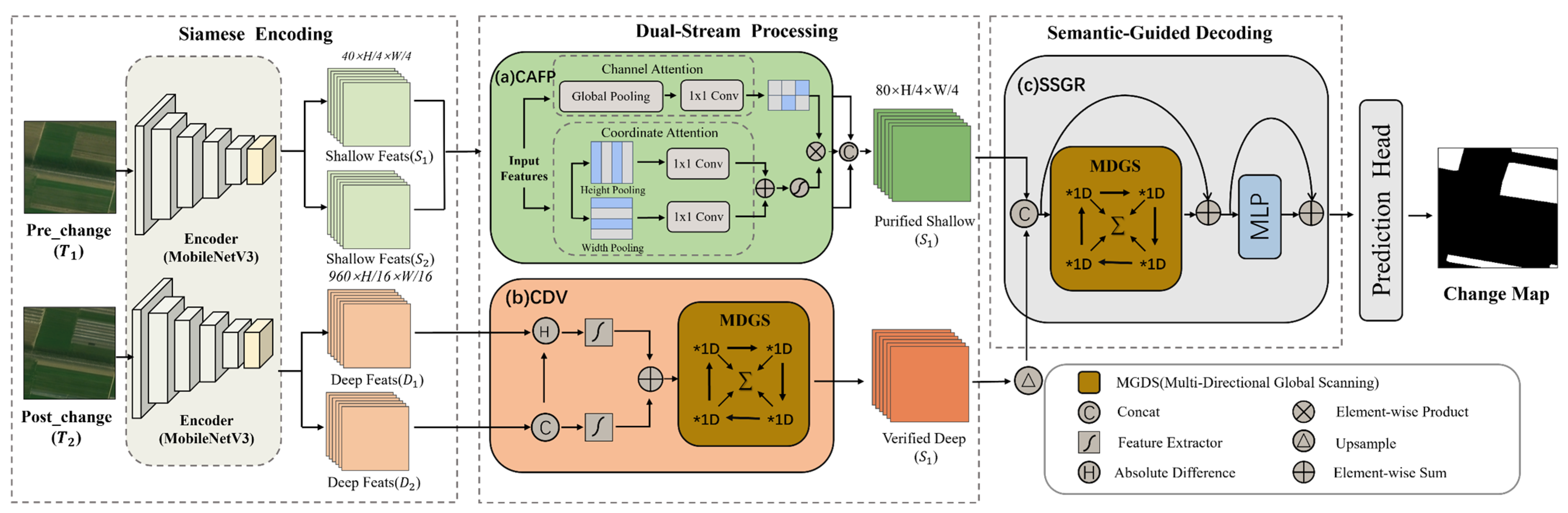
This study proposes LiteScan-Net, a network designed for change detection in high-resolution remote sensing images. The overall architecture of the network is illustrated in Figure 1. The network adopts a Siamese encoder–decoder paradigm. First, a MobileNetV3 [49] backbone, pre-trained on ImageNet [50], is utilized as a weight-sharing encoder to extract multi-level features from the input bi-temporal images (T₁ and T₂). Next, to address background noise interference, these shallow features are fed into the CAFP module for texture refinement. Subsequently, the deep semantic features are processed by the CDV module. To overcome the misalignment of deep semantic features and the limited effective receptive fields of traditional CNNs, the CDV module integrates a novel MDGS mechanism that efficiently captures long-range dependencies and aligns semantic representations. Finally, the SSGR module takes these refined features to reconstruct fine-grained change maps with global consistency. By integrating this scanning mechanism, LiteScan-Net effectively overcomes the inherent locality of traditional CNNs, ensuring robust detection in complex cropland scenarios.

3.2. Coordinate-Aware Feature Purification (CAFP)

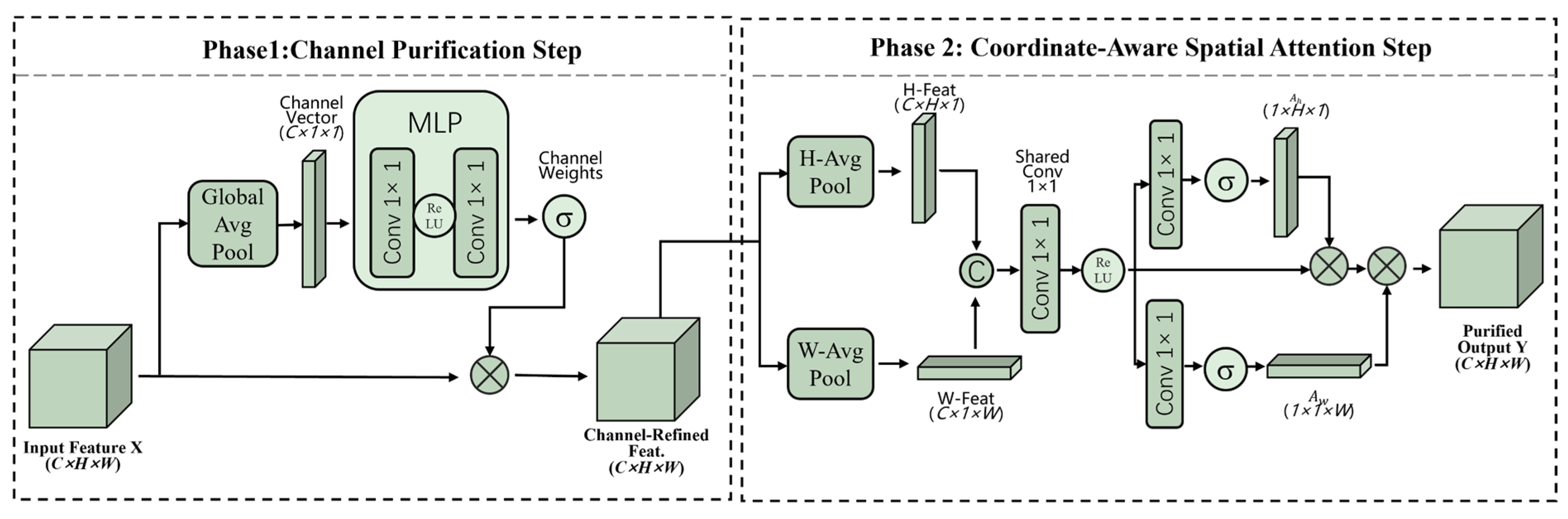
The shallow features extracted from the initial stages of the encoder provide essential high-frequency details for CD; however, they are also contaminated by background noise irrelevant to the task. Conventional attention mechanisms frequently rely on global pooling, which inevitably loses spatial details when compressing information. To mitigate this, we propose the CAFP module—a highly efficient component that jointly refines feature representations along both the channel and spatial dimensions. Its detailed architecture is illustrated in Figure 2.

The CAFP operation consists of two sequential steps: channel attention for feature selection and coordinate attention for precise localization. First, to emphasize semantically rich channels and suppress redundant ones, the input feature $F\in R^{C\times H\times W}$ undergoes global average pooling to aggregate spatial information into a channel descriptor $g\in R^{C\times 1\times 1}$. A gating mechanism is then applied to model channel dependencies:

$$A_c=\sigma \left(W_2\delta \left(W_{1}g\right)\right)$$

(1)

where $W_1$ and $W_2$ represent two $1\times 1$ weights, $\delta$ is the ReLU activation function, $\sigma$ is the Sigmoid function, and $A_c$ is the channel weight vector.

To capture cross-channel interactions while preserving precise positional information, coordinate-aware pooling is introduced. Different from standard global pooling, CAFP aggregates features along the height ($H$) and width ($W$) dimensions separately to retain positional information.

$$g^h\left(h\right)={\displaystyle \frac{1}{W}}\sum _{0\le i\le W}F\left(h,i\right)$$

(2)

$$g^w\left(w\right)={\displaystyle \frac{1}{H}}\sum _{0\le j\le H}F\left(j,w\right)$$

(3)

$$f=\delta \left(F_{conv}\left(\left[g^h,g^w\right]\right)\right)$$

(4)

where $g^h$ and $g^w$ denote the aggregated features along the vertical and horizontal coordinates, respectively. These two are concatenated and processed through a shared 1 × 1 convolution transformation to capture spatial interaction information. The intermediate feature $f$ is then split into $f^h$ and $f^w$. Finally, independent convolutions are used to convert them into attention maps.

$$A_h=\sigma \left({Conv}_h\left(f^h\right)\right)$$

(5)

$$A_w=\sigma \left({Conv}_w\left(f^w\right)\right)$$

(6)

The final purified feature map is obtained by reweighting the input and generating an attention map:

$$F^{\prime }=F⨀A_c⨀A_h⨀A_w$$

(7)

Through this process, CAFP effectively suppresses background noise unrelated to the task while enhancing the boundary response of change targets.

3.3. Multi-Directional Global Scanning Unit (MDGS)

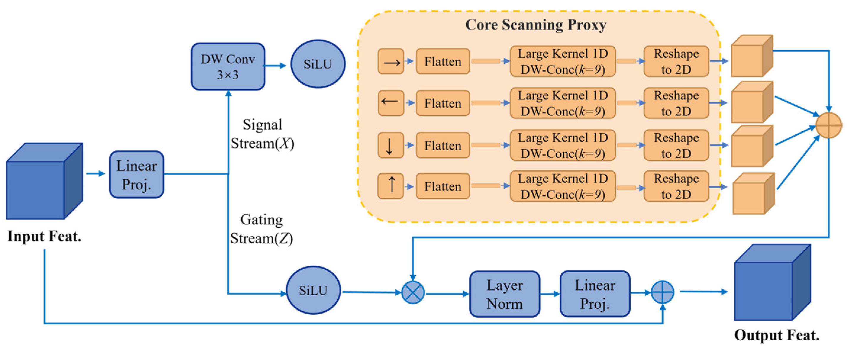
Standard CNNs are restricted by their limited receptive fields, making it difficult to capture long-range semantic dependencies of elongated features such as roads and rivers. To address this with high computational efficiency, we propose the MDGS unit as an engineering surrogate that leverages scanning principles. Its detailed architecture is illustrated in Figure 3.

The MDGS unit, designed as a hardware-friendly proxy for SSM-like behavior, employs efficient convolutional operators to simulate sequential modeling processes. Given an input feature map $X\in R^{C\times H\times W}$, the MDGS unit first projects it into feature branches $V$ and gate branches $Z$, then applies deep convolutions to capture local spatial context.

$$V,Z=Split\left(Linear\left(X\right)\right)$$

(8)

To model 2D spatial context through 1D operations, the feature map $V$ is flattened into 1D sequences along four different directions. Instead of using memory-intensive transpose operations, our flattening strategy is efficiently implemented via spatial flipping and row-major flattening: (1) Standard Path: $V$ is directly flattened row by row, yielding the sequence $V_1$. (2) Horizontal Flip: $V$ is flipped along the width dimension and then flattened row by row (equivalent to right-to-left scanning), yielding $V_2$. (3) Vertical Flip: $V$ is flipped along the height dimension and flattened (equivalent to bottom-to-top scanning), yielding $V_3$. (4) Bi-directional Flip: $V$ is flipped along both height and width dimensions and flattened, yielding $V_4$. Large-kernel 1D convolutions (kernel size = 9) are employed to aggregate information along these sequences:

$$Y_k={Conv1D}_{9\times 1}\left(V_k\right),k\in \left\{\mathrm{1,2},\mathrm{3,4}\right\}$$

(9)

This operation simulates the scanning trajectory typically found in latent state models, enabling each pixel to perceive information from distant regions along the scanning trajectory. To perform the $Unflatten$ operation, the processed 1D sequences $Y_k$ are first reshaped directly back to the 2D spatial dimensions, and then subjected to the exact inverse spatial flipping operations corresponding to their input paths. Finally, the four perfectly aligned 2D feature maps are aggregated via element-wise addition, and adjusted via the gated Z-axis:

$$Y_{out}=LayerNorm\left(\left(\sum _{k=1}^{4}Unflatten\left(Y_k\right)\right)⨀SiLU\left(Z\right)\right)$$

(10)

The fundamental differences between MDGS and VMamba lie in two aspects. First, in terms of computational mechanisms, VMamba’s serialized recursion entails strict sequential state dependencies, which limit parallelization. In contrast, MDGS applies 1D convolutions across four directionally flattened sequences. Its linear operations at all positions are mutually independent and highly parallelizable, completely circumventing hardware bottlenecks. Second, regarding modeling capabilities, VMamba relies on implicit recursion (S6) to achieve dynamic global modeling. MDGS, however, provides a “pseudo-global” receptive field through the static linear operations of multi-directional large-kernel 1D convolutions. This recurrence-free engineering surrogate not only captures the long-range dependencies of elongated features but also better preserves local textural geometries with higher inference efficiency.

3.4. Contextual Difference Verification (CDV)

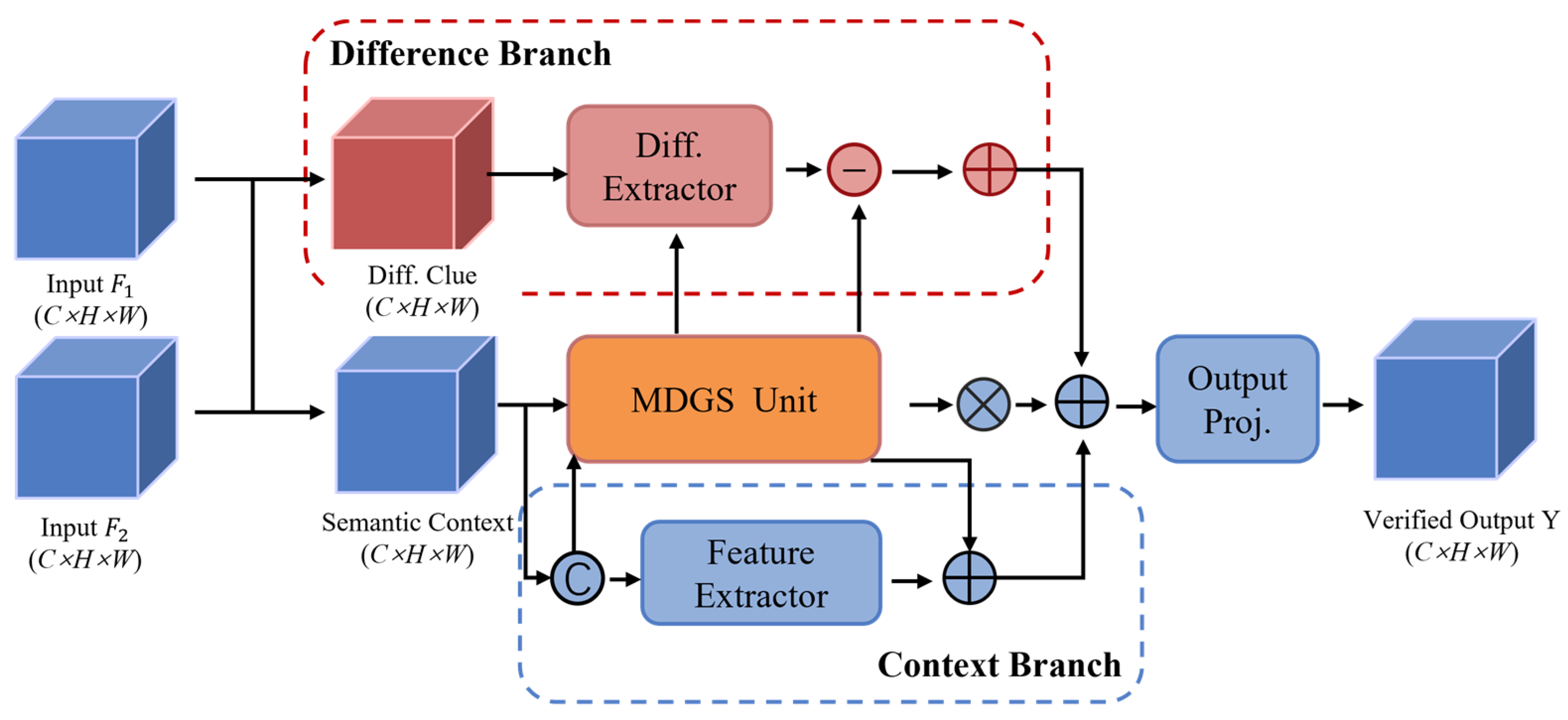
The recognition of genuine changes in deep feature spaces is often disrupted by semantic misalignment caused by off-nadir angle variations and registration errors. Traditional methods employ simple subtraction or concatenation followed by local convolution, lacking the global receptive field required to distinguish structural misalignment from genuine object appearance changes. To address this, we propose the CDV module. Its detailed architecture is illustrated in Figure 4.

The CDV module processes the bi-temporal features to achieve precise verification by fusing explicit differential features with implicit semantic information. Specifically, it calculates the absolute difference map to highlight potential change regions, and concatenates the bi-temporal features to prevent the loss of original semantic information. The core of the module lies in performing global verification through a scanning mechanism. We contend that confirming changes is not a simple superposition of features, but requires verifying the validity of local differences based on global semantics. In this work, we inject differential information into contextual features and feed the fusion results into the MDGS unit.

$$F_{fused}=MDGS\left(F_{diff}+F_{base}\right)$$

(11)

At this stage, the scanning mechanism of the MDGS unit performs the critical role of global verification. By aggregating long-range dependencies, it is intended to help distinguish whether local differences belong to coherent structural changes or isolated noise interference.

3.5. State-Space Guided Rectification (SSGR)

During the decoding phase, conventional approaches aggregate upsampled deep and shallow features through skip connections to restore spatial resolution. However, these two feature types exhibit significant semantic discrepancies: deep features possess high-level semantic information but suffer from low resolution, while shallow features are rich in textural details yet lack semantic coherence. Direct concatenation often leads to feature misalignment, resulting in semantic discontinuities in the final prediction. To address this, we propose the SSGR module, whose detailed structure is shown in Figure 5.

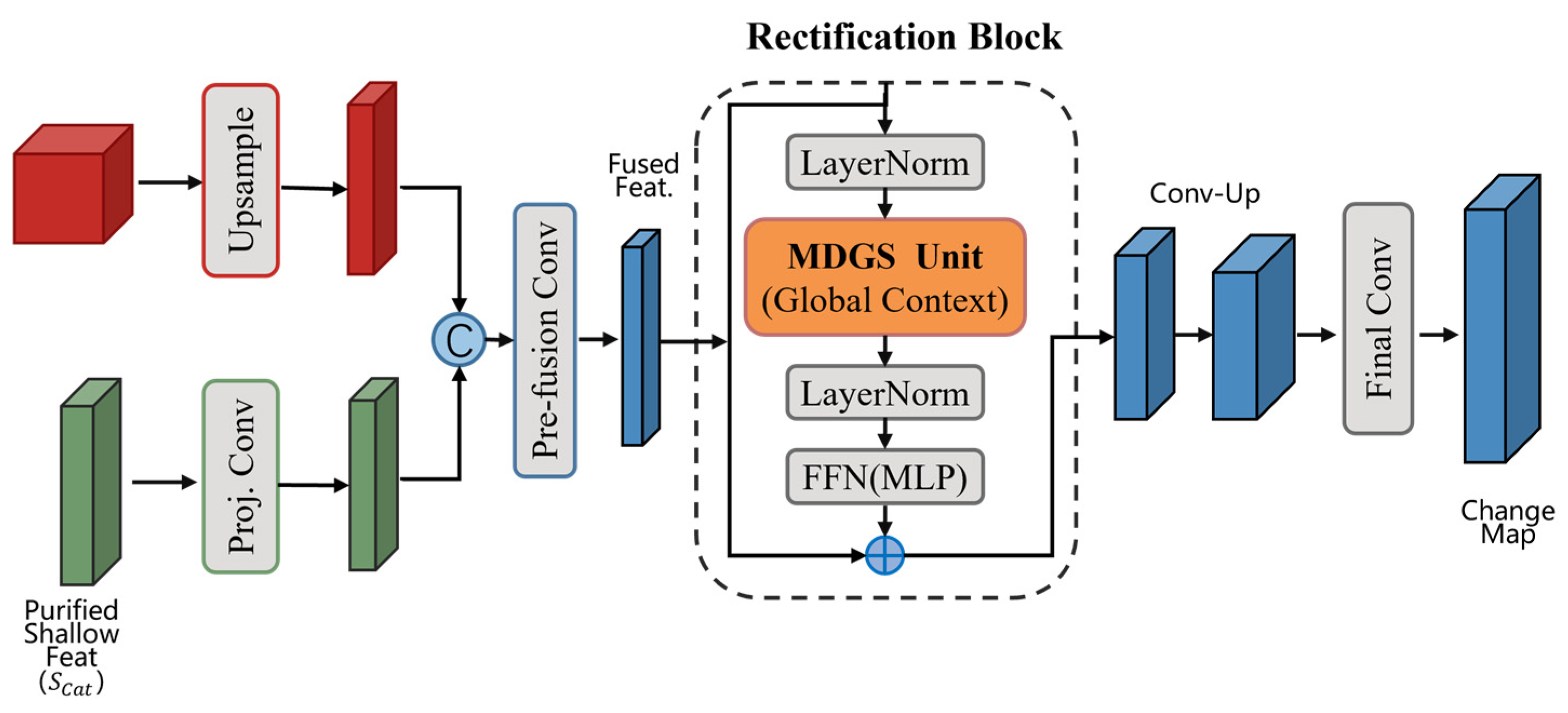
The SSGR module comprises two stages: feature alignment and global optimization. First, the shallow features $F_s$ purified by CAFP and the fused deep features $F_d$ output by CDV are projected onto a unified channel dimension $C$and concatenated to form a fused feature $F_{cat}\in R^{2C\times H\times W}$:

$$F_{cat}=Concat\left(\left[Up\left(F_d\right),{Conv}_{1\times 1}\left(F_s\right)\right]\right)$$

(12)

Then, this concatenated feature map $F_{cat}$ serves as the input to the MDGS module for global rectification. Unlike standard convolutional decoders that perform only local operations, this process utilizes deep, strong semantic context to guide the selection of shallow spatial details, assisting in smoothing semantic discontinuities.

$$F_{refined}=MLP\left(MDGS\left(LayerNorm\left(F_{cat}\right)\right)\right)+F_{cat}$$

(13)

Finally, the optimized features are designed to promote the recovery of target boundaries that are both clear and semantically consistent. By incorporating a prediction head with progressive upsampling and convolutional layers, a final binary change map is generated.

3.6. Loss Function

Class imbalance is one of the core challenges in CD tasks. In remote sensing images, the number of unchanged background pixels is significantly larger than that of changed foreground pixels, resulting in optimization gradients that are frequently dominated by the background. We adopt a hybrid optimization strategy combining weighted Binary Cross-Entropy (BCE) loss and Dice loss to effectively address this issue.

1. Weighted BCE Loss: This is used to measure the discrepancy between the model’s predicted probability distribution and the true label distribution [51]. To balance the contributions of positive and negative samples, category weights are introduced to construct the weighted BCE loss, as follows:

$$L_{bce}=-{\displaystyle \frac{1}{N}}\sum _{i=1}^N\left(\mathrm{\omega }·y_i\log \left(p_i\right)+\left(\left(1-y_i\right)\log \left(1-p_i\right)\right)\right)$$

(14)

where $\omega$ is the hyperparameter for the weight of the enhanced change class, $N$ is the total number of pixels, and $p_i$ and $y_i$ represent the predicted change probability and the true label of the pixel, respectively.

2. Dice Loss: The Dice loss overcomes the limitations of BCE, which focuses solely on pixel-level accuracy, by incorporating the Dice Similarity Coefficient (DSC) [52]. This loss function evaluates the geometric overlap between the predicted region and the ground truth label from a global perspective. It exhibits strong robustness to variations in the scale of foreground objects and is particularly effective for enhancing the integrity of cultivated land parcel boundaries. The formula is as follows:

$$L_{dice}=1-{\displaystyle \frac{2{\sum }_{i=1}^N{y}_i{p}_i+\epsilon }{{\sum }_{i=1}^N{y}_i+{\sum }_{i=1}^N{p}_i+\epsilon }}$$

(15)

where $\epsilon$ is a smoothing term used to prevent the denominator from becoming zero and stabilize the training process. Additionally, 1-DSC transforms the maximizing overlap problem into a minimizing loss problem.

3. The total loss function is designed to balance pixel-level smooth classification with region-level structural consistency. The total loss employed in this study is defined as the weighted sum of both components:

$$L_{total}={{\lambda }_{bce}L}_{bce}+{{\lambda }_{dice}L}_{dice}$$

(16)

where ${\mathrm{\lambda }}_{bce}$ and ${\mathrm{\lambda }}_{dice}$ serve as hyperparameters balancing the weights of the two loss terms. This combined strategy employs BCE optimization for pixel-level accuracy and Dice optimization for global overlap, thereby effectively addressing the challenge of sample imbalance while ensuring boundary precision. In our implementation, both ${\mathrm{\lambda }}_{bce}$ and ${\mathrm{\lambda }}_{dice}$ are set to 1.0 to achieve a balanced optimization.

4. Dataset Description and Experimental Settings

4.1. Datasets

(1)

CLCD Dataset [21]: Contains 600 pairs of farmland change images derived from GF-2 satellite imagery captured in Guangdong Province, China, in 2017 and 2019 [21]. Each image measures 512 × 512 pixels with a spatial resolution ranging from 0.5 to 2 m, enabling clear detection of fine-scale land cover changes within agricultural landscapes. Primary change types include buildings, roads, lakes, and bare land. To strictly rule out the risk of spatial leakage, we first partitioned the original 512 × 512 images into training, validation, and testing sets (in a 3:1:1 ratio) by following the official split criteria. Subsequently, the images within these geographically isolated sets were cropped into 256 × 256-pixel patches for the experiments.

(2)

Hi-CNA Dataset [23]: To further evaluate the model’s performance in identifying the non-agricultural conversion of farmland with high representational consistency, we introduced the Hi-CNA dataset. This dataset is also based on GF-2 satellite imagery and includes visible and near-infrared bands. In the experiments described in this paper, we extracted only the visible (RGB) bands to ensure architectural consistency and a fair comparison, as both LiteScan-Net and the baseline models are optimized for 3-channel inputs. To enhance the model’s discriminative power and increase training difficulty, we specifically focused on the image pairs containing change instances. This design choice is primarily motivated by the inherent class imbalance in cropland change detection; by filtering out patches entirely devoid of changes, we avoid the “performance inflation” effect, where metrics like Overall Accuracy (OA) are artificially inflated by an overwhelming majority of trivial no-change pixels. This strategy avoids the potential inflation of performance metrics caused by a large number of trivial no-change patches, while providing a more rigorous “hard sample mining” environment. Importantly, this strategy does not compromise the model’s ability to learn background representations. Even within these change-positive patches, the actual changed areas occupy only a small fraction of the total pixels. Therefore, the vast remaining non-changing regions within these patches still provide a sufficient and more challenging set of background samples for robust representation learning. While we acknowledge that this setting differs from raw operational conditions where no-change areas dominate, it is essential for evaluating the model’s true discriminative rigor in complex agricultural scenarios. Crucially, the data were partitioned strictly according to the official original split to ensure geographic independence and prevent spatial leakage.

(3)

MSCC Dataset: To precisely capture the process of non-agricultural cropland conversion and address gaps in existing datasets covering agricultural phenological characteristics, we constructed the MSCC dataset. The source imagery was obtained from the GaoFen-2 (GF-2) satellite (PMS sensors, accessible via the China Center for Resources Satellite Data and Application at https://data.cresda.cn/ (accessed on 19 July 2025)), providing a fused spatial resolution of 1.0 m. The spectral composition consists of Red, Green, and Blue (RGB) bands, which were selected to ensure feature consistency across sensors. Spatially, MSCC covers a total acquisition area of 9984.8 $\mathrm{k}{\mathrm{m}}^2$ across diverse agricultural landscapes in typical grain-producing counties of Henan Province, China (e.g., Zhoukou and Kaifeng). Spanning 2024–2025, the dataset comprehensively covers key growth stages of major grain crops such as wheat and corn, including sowing, jointing, grain filling, and harvesting. It documents the non-agricultural conversion of cropland into agricultural facilities, construction land, forest land, water bodies, and roads, as well as ecological restoration processes like cropland reclamation. The construction process involved rigorous preprocessing, including orthorectification and sub-pixel level registration. The annotation was performed by a team of professional interpreters using a dual-check protocol to minimize labeling uncertainty. Furthermore, to quantitatively evaluate the label quality, we conducted an inter-annotator agreement test on a random subset of 500 image pairs. The results yielded an Intersection over Union (IoU) of 95.4%, confirming the high consistency and reliability of the ground truth labels. Ultimately comprising 6000 pairs of 256 × 256 high-resolution images, it stands as one of the most challenging datasets for complex agricultural landscapes today. Crucially, to prevent spatial leakage, the MSCC dataset was also partitioned into training, validation, and testing sets according to a 3:1:1 ratio at the original scene level, ensuring that image patches in the testing set were extracted from geographic locations entirely distinct from those used in the training and validation sets.

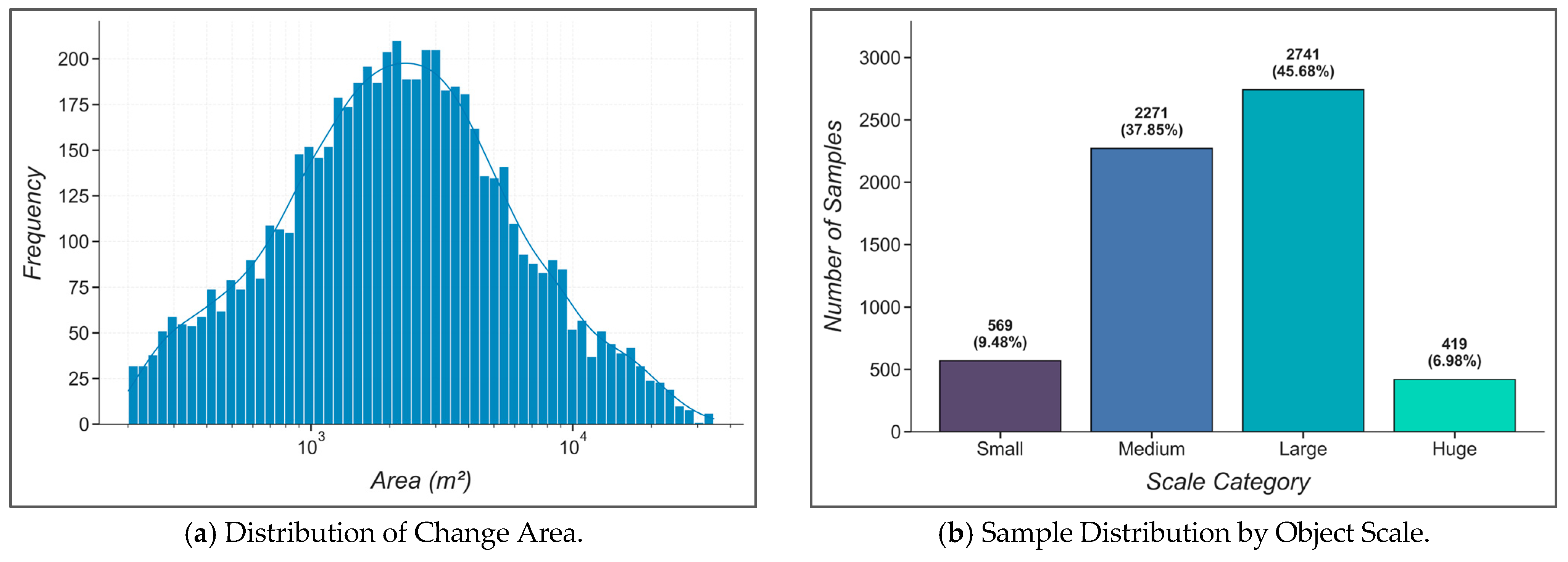
To clarify the difficulties in cropland change detection, a quantitative analysis was conducted on the area distribution characteristics of change instances in the MSCC dataset, and the results are shown in Figure 6. The results indicate that the area of change patches follows a typical log-normal distribution, with a median area of 2147.2 ${\mathrm{m}}^2$. The overall distribution is centered on medium-scale patches, yet a pronounced “long-tail effect” is observed. Statistical results of scale classification show that the dataset is dominated by large-scale (2000–10,000 ${\mathrm{m}}^2$, 45.68%) and medium-scale (500–2000 ${\mathrm{m}}^2$, 37.85%) targets, which effectively represent common scenarios of cropland restructuring. The core challenges arise from targets at both ends of the scale spectrum: small-scale targets are easily filtered out during downsampling due to their weak texture information, while ultra-large-scale targets tend to suffer from hollowing effects as they exceed the convolutional receptive field. This heterogeneous distribution, characterized by “extending at both ends and being dense in the middle,” authentically reflects the coexistence of fragmentation and large-scale transformation in cropland non-agricultural conversion. Thus, MSCC serves as an ideal benchmark for evaluating the multi-scale generalization ability of algorithms in complex agricultural landscapes.

4.2. Comparison Methods

To comprehensively validate the performance of the proposed LiteScan-Net, nine mainstream CD methods were selected as baselines. These methods cover three major categories: CNN-based, Transformer-based, and Mamba-based methods. The specific models are as follows:

FC-EF: As an early benchmark model for deep learning-based CD, the FC-EF model adopts an image-level early fusion strategy. It concatenates bi-temporal images along the channel dimension and feeds them into a fully convolutional network (FCN), preserving spatial details through skip connections [12].

STANet: To address the pseudo-change interference in bi-temporal images, STANet introduces a spatiotemporal attention module during the feature extraction stage of the Siamese network [19]. This module captures extensive spatiotemporal dependencies and enhances the discriminability of features, making STANet a classic application of attention mechanisms in CNNs.

SNUNet: SNUNet integrates the Siamese network with the NestedUNet (UNet++) architecture. By leveraging dense nested skip connections and an integrated channel attention module, it effectively mitigates the loss of localization information in deep networks, serving as a typical case of multi-scale feature fusion currently [53].

SRCNet: SRCNet designs a perception interaction module and a patch-level joint feature fusion module. These modules strengthen the spatial structural correlation of bi-temporal features, solve the problem of insufficient utilization of spatial relationships, and thereby improve detection accuracy [54].

Changer: Emphasizing the critical role of bi-temporal feature interaction, Changer introduces a general change detection architecture equipped with alternating interaction layers. By implementing strategies such as Aggregate-Distribute (AD) and feature exchange, it achieves highly effective alignment and fusion of bi-temporal features, producing robust change predictions [27].

BIT: BIT pioneered the introduction of Transformer into change detection. It marks bi-temporal images as semantic Tokens and models global context in the token space through a Transformer encoder, enhancing the ability to identify target change regions [10].

MSCANet: MSCANet is a typical CNN-Transformer hybrid architecture. It uses CNNs to extract hierarchical features and designs a Transformer-based multi-scale context aggregation module, balancing fine-grained local details and long-range global semantics [21].

ELGC-Net: To address the high computational complexity of Transformer, ELGC-Net proposes an efficient local-global context aggregation strategy. Through pooling transpose attention and depthwise convolution, it significantly reduces the number of parameters while efficiently capturing context information [55].

ChangeMamba: To overcome the limitations of CNN receptive fields and the high computational complexity of Transformers, this method introduces Visual Mamba as its core encoder and designs a specialized spatiotemporal interaction mechanism. It efficiently captures long-range spatiotemporal dependencies across dual-phase images with linear complexity [35].

4.3. Evaluation Metrics

1. Overall Accuracy (OA): As a universal metric for evaluating the global performance of binary classification tasks, OA quantifies the proportion of pixels correctly classified (including both changed and unchanged categories) relative to the total number of pixels in the image. Here, TP, TN, FP, and FN represent true positives, true negatives, false positives, and false negatives, respectively. Its calculation formula is defined as follows:

$$OA={\displaystyle \frac{TP+TN}{TP+FP+TN+FN}}$$

(17)

2. Precision and Recall: These two metrics evaluate the reliability and completeness of the model in detecting changed areas, respectively. Precision measures the model’s ability to suppress false alarms, focusing on the proportion of truly changed pixels among those predicted as changed. Recall measures the model’s ability to avoid omissions, focusing on the proportion of truly changed pixels that are correctly identified:

$$Precision={\displaystyle \frac{TP}{TP+FP}}$$

(18)

$$Recall={\displaystyle \frac{TP}{TP+FN}}$$

(19)

3. F1-score: Given the inherent class imbalance in change detection—where unchanged pixels significantly outnumber changed pixels—a single metric (either Precision or Recall) may yield a biased evaluation. As the harmonic mean of Precision and Recall, the F1-score provides a balanced measure of the model’s ability to minimize both false alarms and omissions. Its calculation formula is defined as:

$$F_1={\displaystyle \frac{2\times Precision\times Recall}{Precision+Recall}}$$

(20)

4. Intersection over Union (IoU): Specifically for the change category, IoU measures the spatial overlap between the predicted change map and the ground-truth label. It is a crucial metric for evaluating segmentation quality, expressed as follows:

$$IoU={\displaystyle \frac{TP}{TP+FP+FN}}$$

(21)

4.4. Experimental Settings

All experiments in this study were implemented using the PyTorch (version 2.2.0) framework, with training conducted on a single NVIDIA GeForce RTX 3090 GPU. To ensure reproducibility and internal consistency, a fixed random seed was employed for all experimental runs. The training hyperparameters were configured as follows: an initial learning rate of 0.001, which was found to be effective for the Adam optimizer’s convergence in our lightweight architecture and was dynamically adjusted using a learning rate decay schedule; the Adam optimizer; a batch size of 8; and a total of 100 epochs. The total loss was calculated as the equally weighted sum of all component losses (with all weighting coefficients set to 1.0) to ensure balanced feature learning across the shallow, deep, and reconstruction stages without introducing hyperparameter bias. To prevent intensive data augmentation from disrupting the spatiotemporal consistency in bi-temporal images, only random horizontal flipping and 90° random rotations were employed. All baseline models were trained using the default configurations recommended in their respective original papers to ensure fairness. Regarding baseline fairness, all models were trained using the default hyperparameter configurations (e.g., learning rate and optimizer settings) recommended in their original papers. Since these baseline architectures are generally size-agnostic regarding their 3-channel input requirements, maintaining the original optimized parameters ensures that the comparison focuses strictly on architectural effectiveness while avoiding potential bias introduced by manual hyperparameter re-tuning. The performance was quantified using five metrics: OA, Precision, Recall, F1-score, and IoU.

4.5. Results of the CLCD Dataset

Table 1. Quantitative Results of Different Methods on the CLCD Dataset.

Model	F1	IoU	Precision	Recall	OA
FC-EF	57.79	40.63	56.29	59.37	93.35
STANet	66.53	49.85	65.03	68.11	94.75
SNUNet	66.91	50.28	73.34	61.52	95.33
SRCNet	70.97	55.00	71.96	70.00	95.61
BIT	76.24	61.61	78.97	73.70	96.48
MSCANet	76.39	61.80	76.55	76.23	96.39
ELGC-Net	67.39	50.82	66.89	67.91	94.96
Changer	70.66	54.64	75.13	66.70	96.58
ChangeMamba	78.91	65.16	77.63	80.23	96.71
Ours	79.43	65.88	79.60	79.27	96.85

presents the evaluation results of the proposed LiteScan-Net against various baseline methods on the CLCD dataset. As observed, our method achieves competitive results in terms of F1, IoU, and Precision, demonstrating the effectiveness of our model in complex change detection scenarios.

Specifically, LiteScan-Net exhibits improved performance in Recall compared to representative hybrid and CNN-based methods such as MSCANet and SNUNet. Traditional CNNs are limited by their receptive fields, making it difficult to capture the complete structures of large change targets. In contrast, our MDGS unit is designed to model long-range dependencies, which contribute to the internal compactness of change masks and substantially reduce missed detections. Meanwhile, the Precision of our model is higher than the Transformer-based method BIT. Although Transformers excel at suppressing global noise, they tend to produce boundary artifacts. In comparison, our CAFP module aims to filter shallow background noise prior to feature fusion. Combined with the SSGR decoder intended for accurate boundary delineation, this assists in reducing false alarms. Additionally, ChangeMamba, based on a spatiotemporal state space model, offers a strong baseline utilizing recursive scanning. In contrast, LiteScan-Net explores an alternative strategy by capturing global context through the recurrence-free MDGS and suppressing shallow interference via CAFP. The results suggest that our lightweight engineering surrogate can achieve performance comparable to more complex state-space models on the CLCD dataset.

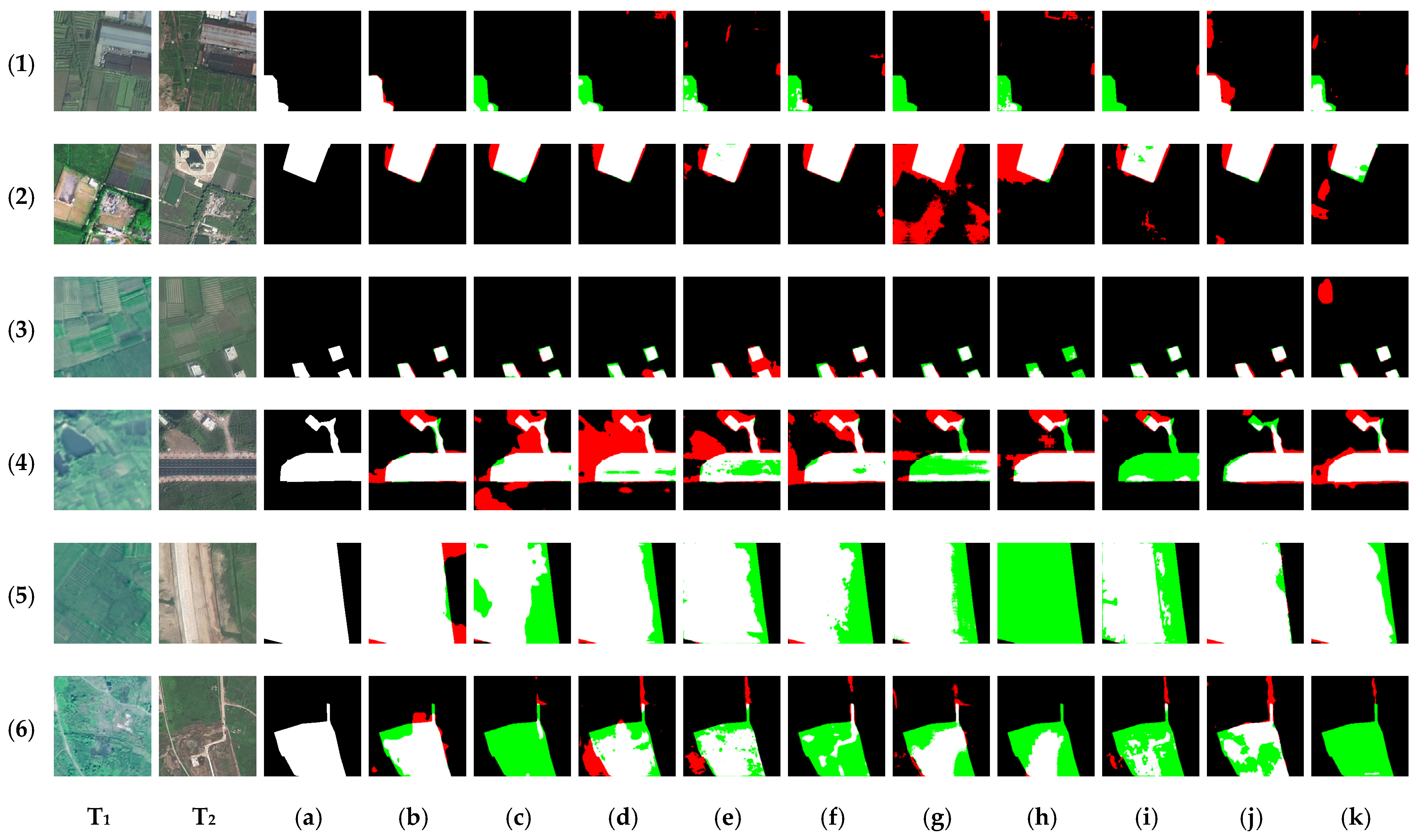
Figure 7 visualizes the detection results of different models, providing a qualitative supplement to the quantitative evaluation of LiteScan-Net. In the small-scale scenarios (1–3), baseline methods such as STANet struggle to capture fine-grained changes (e.g., sporadic low-rise building expansions and local bare land formation) due to shallow noise interference and the limitations of local attention. These targets, characterized by weak textures and small spatial proportions, lead to pronounced false negatives in baseline predictions. In contrast, the design of the CAFP module aims to filter background clutter and noise at the initial feature extraction stage while preserving the high-frequency boundary and positional information of change targets. This is observed to assist in the capture of small-scale, low-contrast changes, yielding results that are spatially consistent with the ground truth.

In the large-scale scenarios (4–6), baseline methods such as SRCNet and SNUNet face challenges in handling continuous changes. Constrained by their limited receptive fields, these traditional CNN-based methods fail to model long-range dependencies and lack sufficient control over global semantic consistency, leading to fragmented and hollowed change masks. In contrast, LiteScan-Net injects differential features into the global context via the CDV module. Leveraging the long-range aggregation capability of the MDGS unit, it validates local discrepancies to distinguish between real changes and registration-induced pseudo-changes. Consequently, LiteScan-Net generates masks with clear boundaries and continuous interiors, presenting a more complete representation of the spatial characteristics of large-scale changes.

4.6. Results of the Hi-CNA Dataset

To further validate the generalization performance of LiteScan-Net across different geographic regions and land feature types, comparative tests were conducted on the Hi-CNA dataset. The quantitative evaluation results are shown in

Table 2. Quantitative Results of Different Methods on the Hi-CNA Dataset.

Model	F1	IoU	Precision	Recall	OA
FC-EF	66.38	49.68	58.22	77.20	81.54
STANet	80.64	67.55	79.86	81.43	90.77
SNUNet	78.92	67.18	78.70	79.14	90.02
SRCNet	81.16	68.29	81.15	81.17	91.11
BIT	82.38	70.05	86.80	78.40	92.09
MSCANet	82.74	70.57	81.45	84.08	91.72
ELGC-Net	81.11	68.23	80.72	81.51	91.04
Changer	80.81	67.81	84.84	77.16	90.93
ChangeMamba	83.22	71.26	81.11	85.43	91.87
Ours	84.82	73.65	86.17	83.52	92.95

. The experimental results indicate that LiteScan-Net consistently achieves superior performance, achieving an F1 score of 84.82% and an IoU of 73.65%. Notably, compared to the CLCD dataset, the performance advantage of the proposed method on Hi-CNA is even more pronounced. Its F1 score outperforms the second-best model, ChangeMamba, by 1.6%, while the precision metric surpasses it by a significant margin of 5.06%. This cross-dataset performance stability demonstrates that the convolutional proxy mechanism possesses excellent feature representation capabilities and generalization robustness when handling diverse remote sensing scenarios, effectively mitigating spectral heterogeneity interference across different regions.

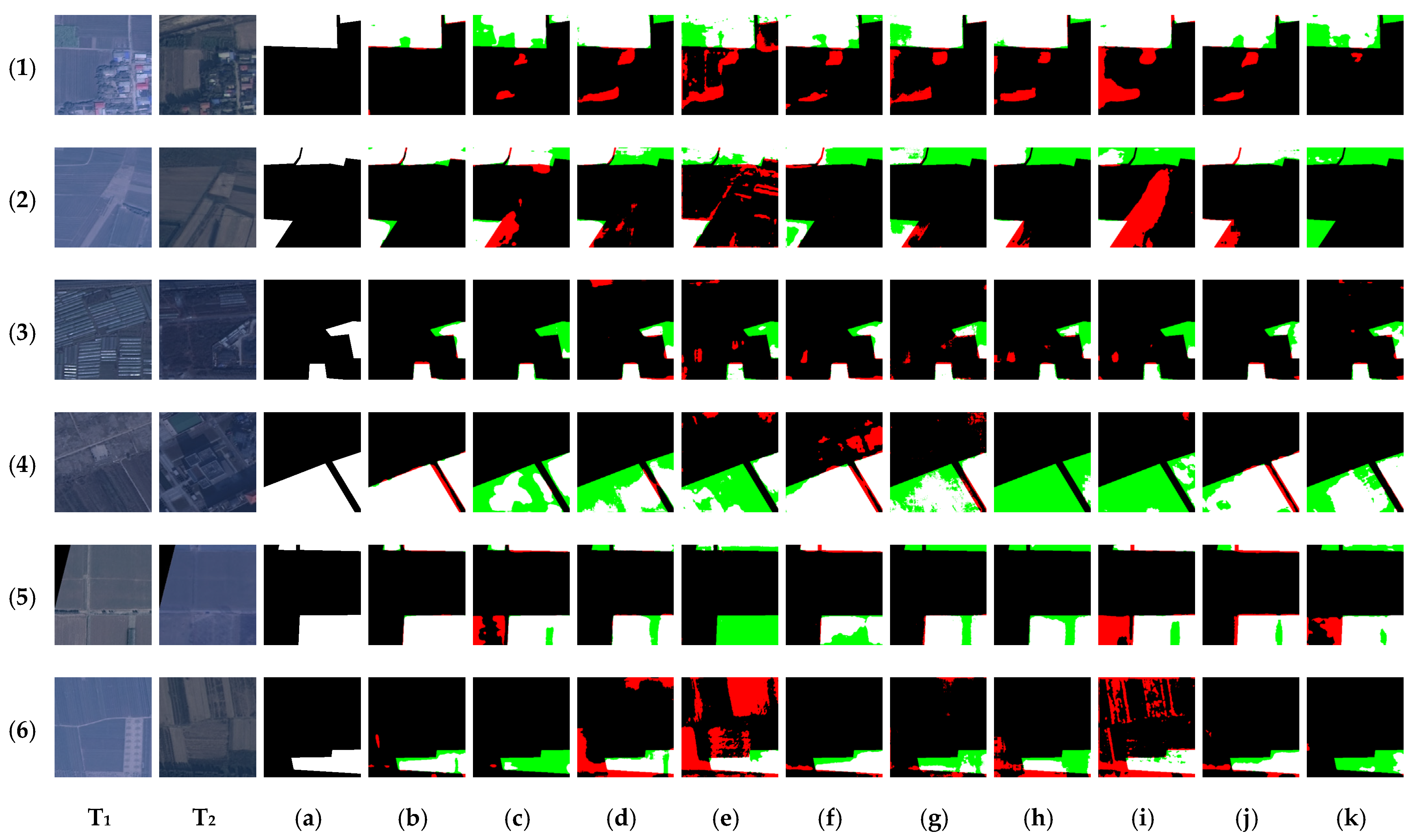
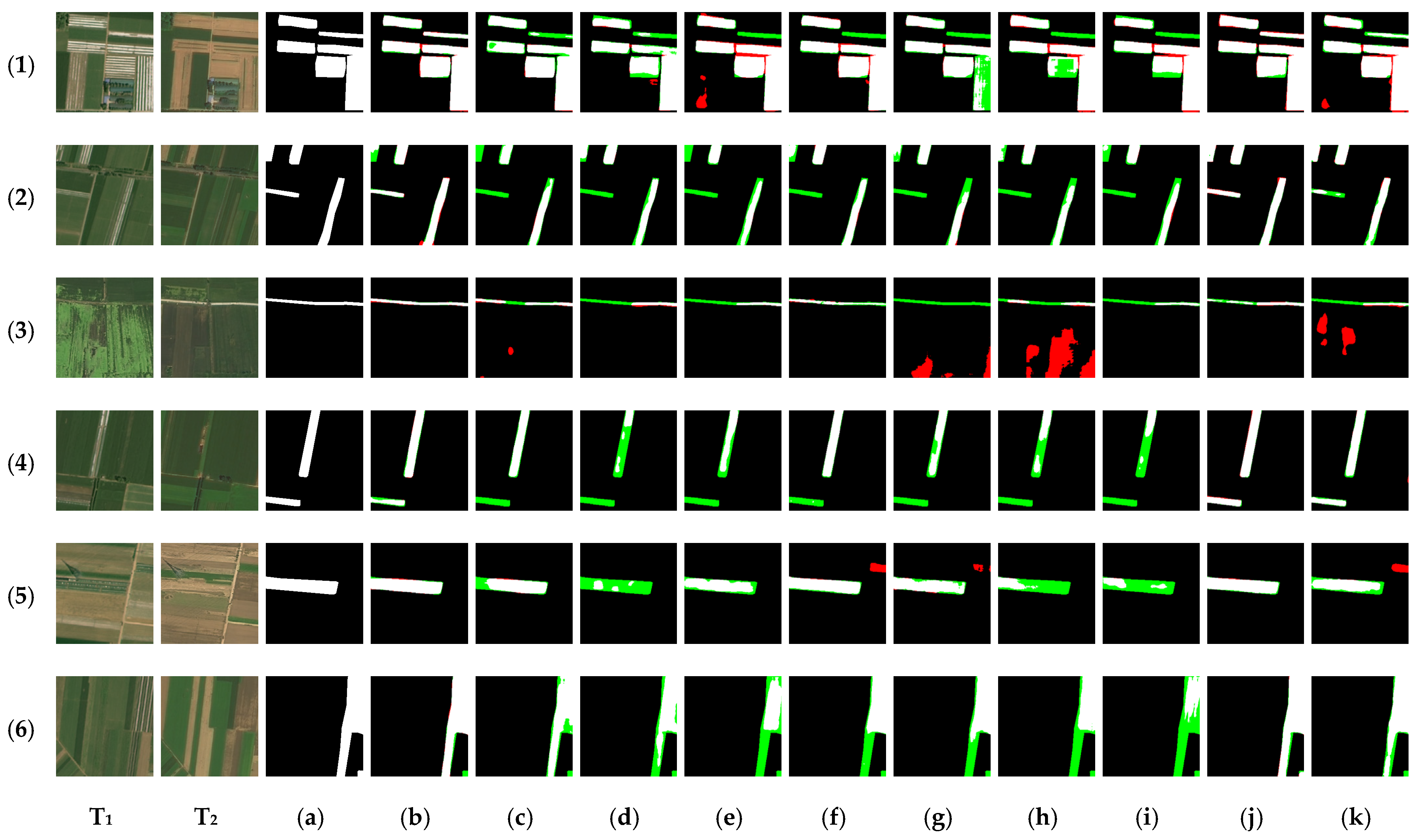
As shown in Figure 8, traditional baseline methods struggle with morphological representation when faced with illumination variations or differences in radiometric characteristics in cross-domain scenarios. In the geometrically complex boundaries shown in cases (1,2), as well as the large-scale contiguous changes in cases (5,6), STANet, FC-EF, and even some Transformer-based methods exhibit noticeable hollowing effects and boundary discontinuities. In contrast, LiteScan-Net appears to generate more compact and internally continuous change masks in these observed cases, with boundaries that align closely with the ground truth labels. Furthermore, in areas with complex background textures, such as cases (3,4), several baseline models are highly susceptible to inter-class spectral confusion, leading to significant false-positive noise. Meanwhile, the proposed model is observed to mitigate pseudo-changes, which is consistent with the context filtering design of its MDGS mechanism. The visualization results illustrate the potential of the proposed network in maintaining spatial consistency and robust generalization performance even when processing out-of-domain data.

4.7. Results of the MSCC Dataset

To further evaluate the generalization capability and robustness of LiteScan-Net, comparative experiments were conducted on the MSCC dataset, with the quantitative results summarized in

Table 3. Quantitative Results of Different Methods on the MSCC Dataset.

Model	F1	IoU	Precision	Recall	OA
FC-EF	69.76	53.56	73.90	66.05	93.83
STANet	82.73	70.54	77.65	88.52	96.02
SNUNet	82.18	70.67	82.42	83.31	96.28
SRCNet	85.99	75.42	83.52	88.61	96.89
BIT	88.63	79.59	89.16	88.11	97.57
MSCANet	88.54	79.44	88.32	88.76	97.52
ELGC-Net	84.09	72.55	84.56	83.63	96.59
Changer	86.23	75.70	87.35	85.13	97.23
ChangeMamba	89.30	80.66	88.73	89.87	97.68
Ours	89.62	81.20	89.36	89.89	97.76

. As shown in Table 3, LiteScan-Net achieves highly competitive results, reaching an F1-score of 89.62% and an IoU of 81.20%. Considering that MSCC exhibits significant scale variability and covers diverse complex agricultural scenarios—ranging from sporadic illegal construction to large-area cropland reclamation—this performance demonstrates that our model can effectively handle various cropland change scenarios with robust performance.

Both the Transformer-based BIT and the SSM architecture-based ChangeMamba demonstrate strong competitiveness, achieving F1 scores of 88.63% and 89.30%, respectively. LiteScan-Net shows comparable performance to these state-of-the-art methods. However, the proposed model surpasses them across all five evaluation metrics. To address the limitations of Transformer models prone to boundary artifacts and ChangeMamba’s susceptibility to potential spatiotemporal noise from recursive scanning, this paper leverages the CAFP module’s coordinate-aware purification capability. This is intended to help filter complex background noise prior to fusion, contributing to a reduction in false alarm rates. Simultaneously, by integrating the multi-directional global scanning mechanism of the MDGS unit, the model aims to capture long-range semantic dependencies to enhance the structural integrity of change targets. This approach potentially assists in preventing internal fragmentation, thereby supporting the reduction of missed detections.

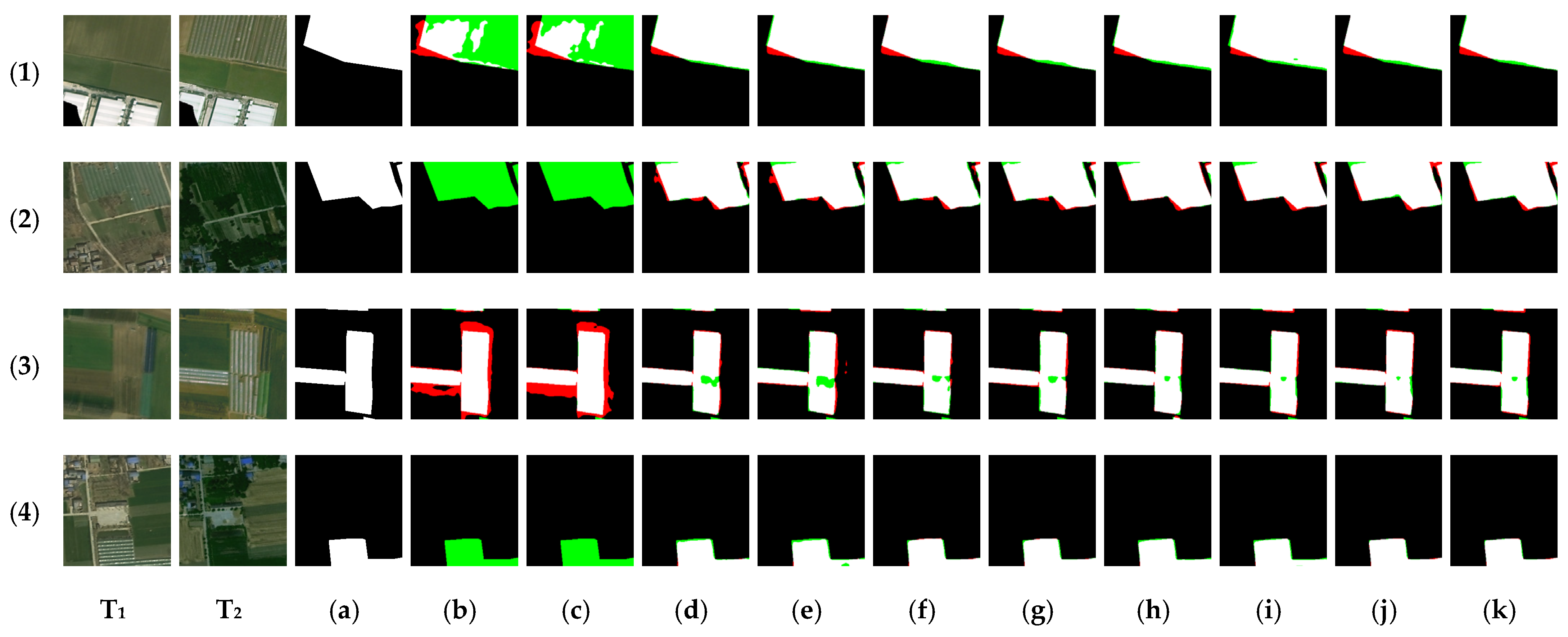
To intuitively demonstrate the detection performance of the model in complex agricultural scenarios, Figure 9 visualizes the inference results of representative samples from the MSCC dataset. As observed, although the baseline models can localize the primary change regions, their predicted boundaries are relatively coarse. In contrast, the change masks generated by LiteScan-Net exhibit more refined edges. Specifically, this spatial refinement is consistent with the design objective of the SSGR module, which is intended to bridge the semantic gap between deep and shallow features through global context constraints. This mechanism facilitates the accurate recovery of shallow spatial details, thereby contributing to the improvement of boundary delineation.

In challenging scenarios where the spectral contrast between change targets and the background is minimal (Figure 9(2–5)), CNN-based methods such as FC-EF and SNUNet struggle to discriminate complete target features, resulting in fragmented predictions and significant omissions. In contrast, LiteScan-Net leverages the robust long-range dependency modeling capacity of the MDGS unit to effectively aggregate global contextual information. While maintaining a high recall rate, it generates complete change masks with improved structural connectivity, suggesting a robust adaptability to complex agricultural scenarios with low contrast. These visual comparisons provide intuitive evidence of enhanced spatial structures, serving as a qualitative supplement to the quantitative metrics reported in the previous sections.

5. Discussion

5.1. Ablation Study

To evaluate the effectiveness and individual contributions of each component in LiteScan-Net, ablation experiments were conducted on the CLCD, Hi-CNA, and MSCC datasets. A baseline model was established for comparison, which employs MobileNetV3 as its backbone, fuses features via simple channel concatenation, and is equipped with a standard upsampling decoder. Starting from this baseline, the three core components (CAFP, CDV, and SSGR) were incrementally incorporated. The quantitative results are summarized in

Table 4. Ablation Study of the LiteScan-Net on the CLCD, Hi-CNA, and MSCC Datasets.

Method			CLCD				Hi-CNA				MSCC
CAFP	CDV	SSGR	F1	IoU	Pre	Rec	F1	IoU	Pre	Rec	F1	IoU	Pre	Rec
×	×	×	76.61	62.08	75.22	78.03	82.80	70.65	85.27	80.48	88.13	78.78	88.15	88.11
√	×	×	78.11	64.09	79.10	77.15	83.80	72.12	85.93	81.78	89.01	80.19	88.96	89.06
×	√	×	78.85	65.09	81.80	76.11	83.53	71.72	87.09	80.25	88.90	80.02	89.54	88.27
×	×	√	79.02	65.32	79.26	78.79	84.24	72.78	85.68	82.86	89.08	80.31	89.02	89.14
√	√	×	79.18	65.52	81.15	77.30	84.35	73.01	86.85	81.98	89.32	80.75	89.35	89.29
√	×	√	79.26	65.65	79.45	79.07	84.58	73.34	86.20	83.02	89.43	80.92	89.20	89.66
×	√	√	79.35	65.78	81.30	77.29	84.65	73.48	86.95	82.47	89.49	81.04	89.42	89.56
√	√	√	79.43	65.88	79.60	79.27	84.82	73.65	86.17	83.52	89.62	81.20	89.36	89.89

‘√’ indicates that the corresponding component (CAFP, CDV, or SSGR) is included in the LiteScan-Net, while ‘×’ indicates that the component is excluded.

.

As observed in Table 4, the progressive integration of each component into the baseline model leads to steady performance improvements. In terms of shallow feature purification, the integration of the CAFP module yields consistent gains across all three datasets: On the CLCD dataset, the Precision is significantly increased to 79.10%; on the Hi-CNA dataset, the F1-score increases from 82.80% to 83.80%; while on the MSCC dataset, the F1-score is improved from 88.13% to 89.01%. Furthermore, the IoU consistently increases by 2.01%, 1.47%, and 1.41% across the three datasets, respectively. The consistent performance gains across three datasets with diverse geographic and phenological characteristics serve as a robust cross-validation of CAFP’s effectiveness. These results confirm that CAFP can effectively filter out shallow background noise and phenological spectral interference, leveraging coordinate-aware attention to enhance representative features.

In terms of deep feature alignment, replacing the simple fusion strategy with the CDV module achieves the highest Precision among all individual modules on all three datasets. (e.g., reaching 81.80% on CLCD). In remote sensing change detection, false positives (lower precision) are the primary manifestation of registration residuals and pseudo-changes. Therefore, this substantial and consistent gain in Precision provides a quantitative indicator of CDV’s mechanism in verifying genuine changes and mitigating alignment-related errors. This suggests that the MDGS-based global scanning mechanism assists in verifying genuine changes, potentially mitigating false positives that often arise from registration residuals or complex phenological variations in agricultural landscapes. However, it is noteworthy that this stringent verification may lead to a marginal trade-off in Recall.

In terms of semantic-guided reconstruction, the SSGR module is crucial for the recovery of fine-grained details: On the MSCC dataset, integrating this module individually achieves a high Recall of 89.14%, which outperforms other single-module variants. Similarly, on the Hi-CNA dataset, the addition of SSGR alone yields the highest F1-score of 84.24% and Recall of 82.86% among the individual module versions. on the CLCD dataset, it maintains a balanced performance with an F1-score of 79.02%. This significant boost in Recall suggests that SSGR effectively recovers fragmented change instances at boundaries that are otherwise overlooked by standard decoders. The performance patterns indicate that global scanning in the decoding stage can help alleviate the “semantic gap” between deep and shallow features, thereby supporting the structural connectivity of change masks.

Furthermore, the evaluation of pairwise combinations (i.e., CAFP + CDV, CAFP + SSGR, and CDV + SSGR) provides critical evidence of the synergistic interaction between the proposed modules. As shown in Table 4, any two-module combination consistently outperforms its single-component counterparts across all metrics. For instance, while the individual CDV module significantly improves Precision, its coupling with SSGR (CDV + SSGR) further boosts the F1-score to 79.35%, 84.65%, and 89.49% on the three datasets, respectively. This incremental improvement demonstrates that the deep feature alignment (precision-oriented) provided by CDV and the detail reconstruction (recall-oriented) of SSGR are highly complementary rather than redundant. Similarly, the CAFP + CDV combination achieves a superior balance in front-end denoising and mid-stage validation, effectively suppressing false positives while maintaining stable Recall.

Finally, by integrating all three modules, LiteScan-Net achieves the best overall performance. Notably, on the MSCC dataset, where the baseline performance was already high, the complete model further improves the F1-score to 89.62% and the Recall to 89.89%, suggesting a synergistic complementarity of the three components. The fact that the full architecture outperforms all pairwise variants confirms that each stage—shallow purification, deep alignment, and semantic reconstruction—is essential and collectively contributes to the model’s robustness. Within this integrated framework, CAFP and CDV are designed to focus on precision through front-end denoising and mid-stage validation, while SSGR aims to assist details in misclassified regions during back-end reconstruction to support improved recall. This results in a robust model that demonstrates effectiveness in complex scenarios (CLCD), consistent non-agricultural conversions (Hi-CNA), and cross-scale scenarios (MSCC).

5.2. Impact of Kernel Size in 1D DW-Conv

To quantitatively analyze the impact of the kernel size $k$ in the 1D DW-Conv within the MDGS module, we evaluated the performance and efficiency of LiteScan-Net under different kernel sizes ($k\in \{1,3,5,7,9,11\}$). The comparative results on the CLCD, Hi-CNA, and MSCC datasets are summarized in

Table 5. Quantitative analysis of different kernel sizes in the MDGS module.

k	Params (M)	FLOPs (G)	CLCD			Hi-CNA			MSCC
			F1	IoU	OA	F1	IoU	OA	F1	IoU	OA
$k=1$	11.741	1.767	76.88	62.44	96.45	83.13	71.12	91.94	87.35	77.55	97.21
$k=3$	11.758	1.770	76.53	61.99	96.30	83.33	71.43	92.14	87.34	77.53	97.25
$k=5$	11.776	1.773	78.28	64.31	96.58	84.09	72.55	92.21	87.97	78.53	97.39
$k=7$	11.793	1.776	75.20	60.25	96.29	83.53	71.72	92.17	87.74	78.15	97.31
$\mathit{k}=9$	11.810	1.780	79.43	65.88	96.85	84.82	73.65	92.95	89.62	81.20	97.76
$k=11$	11.828	1.783	78.56	64.70	96.69	83.50	71.69	92.00	87.43	77.67	97.26

Bold values in each column denote the best performance on the corresponding metric.

.

As illustrated in Table 5, the kernel size $k$ significantly influences the feature representation capability. When $k=1$, the network essentially performs point-wise independent mapping without perceiving local contextual sequences, leading to a suboptimal detection accuracy, such as an F1-score of 76.88% on CLCD. As $k$ increases to 9, the receptive field along the flattened sequences gradually expands, enabling the MDGS to better capture the long-range dependencies of complex features. Consequently, the model achieves its peak performance at $k=9$, attaining an F1-score of 79.43% on CLCD, 84.82% on Hi-CNA, and 89.62% on MSCC.

However, the experimental results clearly indicate that the final performance does not improve indefinitely with the kernel size. When further increasing $k$ to 11, the accuracy exhibits a notable decline, with the F1-score dropping to 78.56% on CLCD, 83.50% on Hi-CNA and 87.43% on MSCC. This performance degradation is consistent with the theory of Effective Receptive Field (ERF) saturation [56,57]. While scaling up the kernel size can theoretically capture broader context, an excessively large 1D receptive field in dense prediction tasks often introduces “context over-smoothing”. In such cases, the excessive integration of heterogeneous regional features or irrelevant background noise tends to overwhelm the fine-grained discriminative features. This phenomenon obscures the precise localization of change boundaries—a critical requirement for cropland monitoring—where the trade-off between global context and local structural integrity must be carefully balanced [58].

To further elucidate the rationale behind the perceptual field trade-off, we critically compared LiteScan-Net with several mainstream approaches. Unlike large-kernel CNNs such as RepLKNet [57] and ConvNeXt [58], which use 2D convolutional kernels (e.g., 31 × 31) to mimic the global perception of Transformers, our results indicate that 1D convolutional kernels with k > 9 introduce excessive noise from heterogeneous backgrounds in fragmented agricultural landscapes. This observation aligns with the local attention mechanism in Swin Transformer [59], but our 1D DW-Conv maintains a lower computational cost. Furthermore, while Transformer-based change detection models like BIT [10] utilize self-attention mechanisms to mitigate spurious changes through global dependencies, LiteScan-Net achieves equivalent robustness against phenological and registration noise by leveraging the sequential scanning characteristics of the MDGS module. By replacing heavy 2D global attention with lightweight 1D scanning, LiteScan-Net achieves a better balance between the long-range modeling capabilities represented by ChangeMamba [35] and the local spatial precision required for fine-grained boundary reconstruction.

Furthermore, regarding computational efficiency, Table 5 demonstrates that owing to the utilization of 1D depth-wise convolutions rather than standard 2D convolutions, the growth in parameters and FLOPs across different $k$ values is extremely marginal. Specifically, scaling $k$ from 1 to 11 only introduces an increment of approximately 0.08 M parameters. Specifically, the FLOPs increase steadily from 1.767 G ($k=1$) to 1.783 G ($k=11$), following the expected logical trend of depth-wise operations.

5.3. Mechanism Validation and Analysis

To validate the specific mechanisms of the proposed module, this study conducted a quantitative analysis of ablation variants through controlled experiments (

Table 6. Quantitative validation of the proposed mechanisms.

Model	CAFP			CDV			SSGR			Stat Rigor
	Prec	Rec	F1	${\mathit{P}}_{\mathit{n}\mathit{o}\mathit{r}\mathit{m}}$	${\mathit{P}}_{\mathit{s}\mathit{h}\mathit{i}\mathit{f}\mathit{t}}$	$∆\mathit{P}$	${\mathit{P}}_{\mathit{b}\mathit{n}\mathit{d}}$	${\mathit{R}}_{\mathit{b}\mathit{n}\mathit{d}}$	B-IoU	$\mathit{F}1 \pm \mathit{S}\mathit{t}\mathit{d}$
baseline	80.74	20.26	32.39	56.78	55.94	−0.84	30.91	12.16	9.56	±0.91
+CAFP	97.64	94.24	95.91	86.67	86.40	−0.27	62.50	64.09	46.29	±0.72
+CDV	97.09	94.45	95.75	88.53	88.32	−0.22	66.48	66.19	49.63	±0.70
+SSGR	94.67	96.38	95.52	87.74	87.38	−0.36	67.67	68.09	51.37	±0.71
LiteScan-Net	96.71	96.30	96.50	88.08	87.93	−0.15	67.99	67.92	51.46	±0.68

). In the validation against phenological interference, using a phenological subset of the MSCC dataset for testing, the Baseline achieved an F1 score of only 32.39% on this subset, whereas the introduction of the CAFP module boosted the F1 score to 95.91%, demonstrating that CAFP can effectively filter out shallow phenological noise caused by seasonal spectral variations. Robustness validation against registration errors showed that under 2-pixel spatial offset interference, the Baseline’s precision dropped by 0.84%, whereas using the CDV module alone limited the model’s degradation to within 0.22%, and the full LiteScan-Net model saw only a 0.15% decline, confirming the effectiveness of the contextual difference verification mechanism in mitigating registration artifacts through global scanning. Furthermore, geometric fidelity evaluations indicate that the SSGR module improves the Boundary Intersection Overlap (B-IoU) from 9.56% in the Baseline to 51.37%, with LiteScan-Net achieving 51.46%, confirming the central role of state-space-guided reconstruction in refined boundary restoration. Finally, based on estimates from 1000 bootstrap resamples, the standard deviation of the full model is only ±0.68%, ensuring the statistical rigor of the experimental conclusions.

To further visually validate the performance gains contributed by each module, this study selected four sets of typical cases from the MSCC dataset for comparative analysis (Figure 10). Cases (1,2): The Baseline model generated clusters of green false positive (FP) pixels in areas of variation, reflecting its extreme sensitivity to spectral fluctuations; however, after introducing the CAFP module, the model accurately identified and filtered out shallow texture noise through a coordinate-aware purification mechanism, resulting in a cleaner error map in the background areas. In the registration offset stress test of Case (3), the Baseline model exhibited continuous FP errors along the edges of displaced objects, whereas the variant equipped with the CDV module effectively suppressed false change responses caused by sub-pixel offsets by leveraging its global context verification capability. Case (4) focuses on farmland boundaries with complex geometric contours. The Baseline suffers from significant loss of edge pixels due to the loss of deep-level features, whereas the SSGR module, through a state-space-guided reconstruction process, accurately recovers the lost boundary details, resulting in a mask edge that closely aligns with the ground truth. Through the synergistic interaction of these three mechanisms, LiteScan-Net achieves the lowest false negatives and false positives across all cases, intuitively demonstrating the robustness of the proposed architecture in complex agricultural remote sensing environments.

5.4. Model Efficiency

To evaluate the practical deployment potential of LiteScan-Net on resource-constrained edge devices, its computational efficiency was compared with other SOTA methods. The evaluation metrics include the number of parameters (Params), floating-point operations (FLOPs), and frames per second (FPS). All tests were conducted on a single NVIDIA GeForce RTX 3090 GPU with an input size of 256 × 256, and the results are summarized in

Table 7. Efficiency Comparison of Different Methods.

Model	Params (M)	FLOPs (G)	FPS	Latency (ms)
FC-EF	1.351	3.577	195.8	5.11
STANet	16.897	12.862	82.9	12.07
SNUNet	12.035	54.833	32.0	31.30
SRCNet	5.195	47.565	36.4	27.44
BIT	11.987	26.310	84.5	11.83
MSCANet	16.592	14.745	37.5	26.65
ELGC-Net	10.572	187.834	21.4	46.80
Changer	11.39	5.955	98.11	10.19
ChangeMamba	49.940	114.820	15.6	64.01
Ours	11.811	1.780	37.9	26.38

.

As shown in Table 7, although the parameter count of LiteScan-Net (11.81 M) is comparable to mainstream models such as BIT (11.98 M) and SNUNet (12.03 M), its core lightweight advantage lies in the extreme reduction in computational complexity (FLOPs). LiteScan-Net requires only 1.78 G of computational overhead, representing a dramatic reduction of 93.2% and 96.7% compared to BIT and SNUNet, respectively. Particularly, when compared to the recent SSM-based ChangeMamba, LiteScan-Net utilizes less than a quarter of the parameters and achieves a staggering 98.4% reduction in FLOPs, successfully breaking the heavy deployment bottleneck of native Mamba models. Remarkably, even when compared to the simplest baseline model FC-EF, which has only 1.35 M parameters, the computational cost of our model is less than half of it. Combined with the accuracy performance in Table 1 and Table 2, our model achieves the highest F1-score (89.62%) on MSCC while consuming the least computational resources. This demonstrates that for resource-constrained edge devices like UAVs, where power consumption and processing capacity are critical bottlenecks rather than just storage space, LiteScan-Net offers a competitive trade-off among memory footprint, computational load, and detection accuracy, suggesting potential for future edge-device integration.

While maintaining high accuracy, LiteScan-Net achieves 37.9 FPS, substantial outperforming complex multi-scale networks such as ELGC-Net, SNUNet, and the computationally heavy ChangeMamba. Although the current scanning mechanism relies on PyTorch native operators, leading to high memory access costs and thus preventing FPS from increasing linearly with reduced FLOPs, 37.9 FPS far exceeds the real-time threshold of 30 FPS. Combined with the extremely low FLOPs, this confirms that LiteScan-Net, as a solution balancing high accuracy and low latency, holds extremely high practical value for deployment on resource-constrained devices.

6. Conclusions

To address the core contradiction in high-resolution remote sensing change detection—where CNNs are limited by local receptive fields and Transformers suffer from high computational costs—we proposed LiteScan-Net, a lightweight and robust model tailored for agricultural monitoring. The core innovation of LiteScan-Net lies in the Multi-Directional Global Scanning (MDGS) mechanism, which simulates the selective scanning process of state space models using large-kernel 1D depthwise convolutions. This achieves global context modeling with linear complexity, effectively balancing global information capture with computational efficiency.

To fully exploit the advantages of MDGS, a three-stage collaborative architecture was constructed. The CAFP, CDV, and SSGR modules perform their respective functions in shallow denoising, deep alignment, and detail reconstruction. Experimental results demonstrate that LiteScan-Net achieves competitive performance compared to mainstream CNN-based and Transformer-based methods across multiple benchmarks, including the CLCD and Hi-CNA datasets, as well as the newly constructed MSCC dataset. Notably, the model achieves a balance between Precision and Recall, enabling the generation of high-quality change masks with improved structural connectivity and clear boundaries. Efficiency analysis further illustrates its potential value: the extremely low computational cost and parameter count make it potentially suitable for deployment on resource-constrained edge devices such as UAVs.

Furthermore, we construct the large-scale, high-precision MSCC dataset dedicated to cropland change detection. This dataset systematically covers a variety of complex agricultural change types, ranging from sporadic illegal construction to large-area reclamation. It effectively mitigates the lack of coverage of cropland scenarios in existing public datasets, thereby providing essential data support for the field of agricultural remote sensing change detection. Despite these advantages, this study has several limitations. First, while the model is theoretically lightweight, its actual inference latency and energy consumption on specific embedded hardware have yet to be empirically verified. Second, the current evaluation predominantly relies on standard pixel-wise metrics, which may not fully capture the nuance of boundary topological consistency in highly fragmented agricultural plots. Furthermore, while our full factorial ablation study provides indirect evidence, the proposed mechanisms—such as CAFP for phenological denoising and CDV for misalignment mitigation—are currently undergoing further validation through dedicated controlled stress tests (e.g., misregistration or explicit phenology-shift analysis). Additionally, we intend to extend this architecture to multi-modal remote sensing change detection to further explore its potential.

References

1. Xiong, Y.; Liu, M.; Wen, L.; Zhang, A. Does urbanization inevitably exacerbate cropland pressure? The multiscale evidence from China. J. Clean. Prod. 2025, 504, 145413. [Google Scholar] [CrossRef] [Scilit]
2. Bren d’Amour, C.; Reitsma, F.; Baiocchi, G.; Barthel, S.; Güneralp, B.; Erb, K.-H.; Haberl, H.; Creutzig, F.; Seto, K.C. Future urban land expansion and implications for global croplands. Proc. Natl. Acad. Sci. USA 2017, 114, 8939–8944. [Google Scholar] [CrossRef] [Scilit]
3. Shafique, A.; Cao, G.; Khan, Z.; Asad, M.; Aslam, M. Deep Learning-Based Change Detection in Remote Sensing Images: A Review. Remote Sens. 2022, 14, 871. [Google Scholar] [CrossRef] [Scilit]
4. Das, S.; Angadi, D.P. Land use land cover change detection and monitoring of urban growth using remote sensing and GIS techniques: A micro-level study. GeoJournal 2022, 87, 2101–2123. [Google Scholar] [CrossRef] [Scilit]
5. Lunetta, R.S.; Knight, J.F.; Ediriwickrema, J.; Lyon, J.G.; Worthy, L.D. Land-cover change detection using multi-temporal MODIS NDVI data. Remote Sens. Environ. 2006, 105, 142–154. [Google Scholar] [CrossRef] [Scilit]
6. Ferraris, V.; Dobigeon, N.; Wei, Q.; Chabert, M. Detecting Changes Between Optical Images of Different Spatial and Spectral Resolutions: A Fusion-Based Approach. IEEE Trans. Geosci. Remote Sens. 2018, 56, 1566–1578. [Google Scholar] [CrossRef]
7. Liu, Q.; Hang, R.; Song, H.; Li, Z. Learning Multiscale Deep Features for High-Resolution Satellite Image Scene Classification. IEEE Trans. Geosci. Remote Sens. 2018, 56, 117–126. [Google Scholar] [CrossRef] [Scilit]
8. Prendes, J.; Chabert, M.; Pascal, F.; Giros, A.; Tourneret, J.-Y. A New Multivariate Statistical Model for Change Detection in Images Acquired by Homogeneous and Heterogeneous Sensors. IEEE Trans. Image Process. 2015, 24, 799–812. [Google Scholar] [CrossRef] [Scilit] [PubMed]
9. Ji, S.; Wei, S.; Lu, M. Fully Convolutional Networks for Multisource Building Extraction From an Open Aerial and Satellite Imagery Data Set. IEEE Trans. Geosci. Remote Sens. 2019, 57, 574–586. [Google Scholar] [CrossRef] [Scilit]
10. Chen, H.; Qi, Z.; Shi, Z. Remote Sensing Image Change Detection with Transformers. IEEE Trans. Geosci. Remote Sens. 2022, 60, 1–14. [Google Scholar] [CrossRef] [Scilit]
11. Wang, H.; Zhuang, P.; Zhang, X.; Li, J. DBMGNet: A Dual-Branch Mamba-GCN Network for Hyperspectral Image Classification. IEEE Trans. Geosci. Remote Sens. 2025, 63, 1–17. [Google Scholar] [CrossRef] [Scilit]
12. Daudt, R.C.; Saux, B.L.; Boulch, A. Fully Convolutional Siamese Networks for Change Detection. arXiv 2018, arXiv:1810.08462. [Google Scholar] [CrossRef] [Scilit]
13. Qiu, J.; Liu, W.; Zhang, X.; Li, E.; Zhang, L.; Li, X. DED-SAM: Adapting Segment Anything Model 2 for Dual Encoder–Decoder Change Detection. IEEE J. Sel. Top. Appl. Earth Obs. Remote Sens. 2025, 18, 995–1006. [Google Scholar] [CrossRef] [Scilit]
14. Wang, L.; Li, R.; Zhang, C.; Fang, S.; Duan, C.; Meng, X.; Atkinson, P.M. UNetFormer: A UNet-like transformer for efficient semantic segmentation of remote sensing urban scene imagery. ISPRS J. Photogramm. Remote Sens. 2022, 190, 196–214. [Google Scholar] [CrossRef] [Scilit]
15. Vaswani, A.; Shazeer, N.; Parmar, N.; Uszkoreit, J.; Jones, L.; Gomez, A.N.; Kaiser, Ł.; Polosukhin, I. Attention Is All You Need. In Proceedings of the Advances in Neural Information Processing Systems; Curran Associates, Inc.: Red Hook, NY, USA, 2017; Volume 30. [Google Scholar]
16. Gu, A.; Dao, T. Linear-Time Sequence Modeling with Selective State Spaces. arXiv 2024, arXiv:2312.00752. [Google Scholar]
17. Zhu, L.; Liao, B.; Zhang, Q.; Wang, X.; Liu, W.; Wang, X. Vision Mamba: Efficient Visual Representation Learning with Bidirectional State Space Model. arXiv 2024, arXiv:2401.09417. [Google Scholar] [CrossRef] [Scilit]
18. Tian, S.; Ma, A.; Zheng, Z.; Zhong, Y. Hi-UCD: A Large-scale Dataset for Urban Semantic Change Detection in Remote Sensing Imagery. arXiv 2020, arXiv:2011.03247. [Google Scholar]
19. Chen, H.; Shi, Z. A Spatial-Temporal Attention-Based Method and a New Dataset for Remote Sensing Image Change Detection. Remote Sens. 2020, 12, 1662. [Google Scholar] [CrossRef] [Scilit]
20. Shen, L.; Lu, Y.; Chen, H.; Wei, H.; Xie, D.; Yue, J.; Chen, R.; Lv, S.; Jiang, B. S2Looking: A Satellite Side-Looking Dataset for Building Change Detection. Remote Sens. 2021, 13, 5094. [Google Scholar] [CrossRef] [Scilit]
21. Liu, M.; Chai, Z.; Deng, H.; Liu, R. A CNN-Transformer Network With Multiscale Context Aggregation for Fine-Grained Cropland Change Detection. IEEE J. Sel. Top. Appl. Earth Obs. Remote Sens. 2022, 15, 4297–4306. [Google Scholar] [CrossRef] [Scilit]
22. Tundia, C.; Kumar, R.; Damani, O.; Sivakumar, G. FPCD: An Open Aerial VHR Dataset for Farm Pond Change Detection. arXiv 2023, arXiv:2302.14554. [Google Scholar] [CrossRef] [Scilit]
23. Sun, Z.; Zhong, Y.; Wang, X.; Zhang, L. Identifying cropland non-agriculturalization with high representational consistency from bi-temporal high-resolution remote sensing images: From benchmark datasets to real-world application. ISPRS J. Photogramm. Remote Sens. 2024, 212, 454–474. [Google Scholar] [CrossRef] [Scilit]
24. Shangguan, Y.; Li, J.; Chen, Z.; Ren, L.; Hua, Z. Multiscale Attention Fusion Graph Network for Remote Sensing Building Change Detection. IEEE Trans. Geosci. Remote Sens. 2024, 62, 1–18. [Google Scholar] [CrossRef] [Scilit]
25. Song, X.; Hua, Z.; Li, J. Remote Sensing Image Change Detection Transformer Network Based on Dual-Feature Mixed Attention. IEEE Trans. Geosci. Remote Sens. 2022, 60, 1–16. [Google Scholar] [CrossRef] [Scilit]
26. Zhang, Y.; Song, X.; Hua, Z.; Li, J. CGMMA: CNN-GNN Multiscale Mixed Attention Network for Remote Sensing Image Change Detection. IEEE J. Sel. Top. Appl. Earth Obs. Remote Sens. 2024, 17, 7089–7103. [Google Scholar] [CrossRef] [Scilit]
27. Fang, S.; Li, K.; Li, Z. Changer: Feature Interaction is What You Need for Change Detection. IEEE Trans. Geosci. Remote Sens. 2023, 61, 1–11. [Google Scholar] [CrossRef] [Scilit]
28. Wu, Q.; Huang, L.; Tang, B.-H.; Cheng, J.; Wang, M.; Zhang, Z. CroplandCDNet: Cropland Change Detection Network for Multitemporal Remote Sensing Images Based on Multilayer Feature Transmission Fusion of an Adaptive Receptive Field. Remote Sens. 2024, 16, 1061. [Google Scholar] [CrossRef] [Scilit]
29. Wu, Q.; Huang, L.; Tang, B.-H. Spatial Location-Guided Global Context Modeling Network for Cropland Dynamic Monitoring in Multitemporal Remote Sensing Images. IEEE J. Sel. Top. Appl. Earth Obs. Remote Sens. 2025, 18, 27549–27564. [Google Scholar] [CrossRef] [Scilit]
30. Lv, J.; Qian, Y.; Bai, L.; Li, C.; Luo, X.; Sang, Y.; Yang, X.; Gong, W. STMTNet: Spatio-Temporal Multiscale Triad Network for Cropland Change Detection in Remote Sensing Images. IEEE J. Sel. Top. Appl. Earth Obs. Remote Sens. 2025, 18, 26005–26020. [Google Scholar] [CrossRef] [Scilit]
31. Duan, M.; Wang, Y.; Bai, L.; He, Y.; Zhao, Z.; Qian, Y.; Liu, X. CAFENet: Change-Aware and Fourier Feature Exchange Network for Cropland Change Detection in Remote Sensing Images. IEEE Geosci. Remote Sens. Lett. 2025, 22, 1–5. [Google Scholar] [CrossRef] [Scilit]
32. Mei, L.; Huang, A.; Ye, Z.; Yalikun, Y.; Wang, Y.; Xu, C.; Yang, W.; Li, X. STLNet: Symmetric Transformer Learning Network for Remote Sensing Image Change Detection. IEEE J. Sel. Top. Appl. Earth Obs. Remote Sens. 2025, 18, 2655–2667. [Google Scholar] [CrossRef] [Scilit]
33. Du, Q.; Zhang, S.; Zhang, N.; Shen, C.; Du, Z.; Guo, X.; Zhao, J. A multiscale siamese transformer attention network for remote sensing image change detection. Earth Sci. Inf. 2025, 19, 5. [Google Scholar] [CrossRef] [Scilit]
34. Zhang, Y.; Yang, L.; Zhu, L.; Zhou, C.; Nanehkaran, Y.A.; Wang, J. A Deep Supervised Change Detection Network Based on Context-Rich Information. IEEE J. Sel. Top. Appl. Earth Obs. Remote Sens. 2025, 18, 21564–21577. [Google Scholar] [CrossRef] [Scilit]
35. Chen, H.; Song, J.; Han, C.; Xia, J.; Yokoya, N. ChangeMamba: Remote Sensing Change Detection With Spatiotemporal State Space Model. IEEE Trans. Geosci. Remote Sens. 2024, 62, 1–20. [Google Scholar] [CrossRef] [Scilit]
36. Chen, K.; Chen, B.; Liu, C.; Li, W.; Zou, Z.; Shi, Z. RSMamba: Remote Sensing Image Classification With State Space Model. IEEE Geosci. Remote Sens. Lett. 2024, 21, 1–5. [Google Scholar] [CrossRef] [Scilit]
37. Gao, R.; Feng, Q.; Cao, J.; Feng, X.; Wang, J.; Yan, L. Crossmodal Hierarchical Heterogeneous Graph Guided Mamba Network for remote sensing semantic segmentation. Clust. Comput. 2025, 29, 20. [Google Scholar] [CrossRef] [Scilit]
38. Yan, L.; He, Z.; Zhang, Z.; Xie, G. LS-MambaNet: Integrating Large Strip Convolution and Mamba Network for Remote Sensing Object Detection. Remote Sens. 2025, 17, 1721. [Google Scholar] [CrossRef] [Scilit]
39. Zhou, S.; Xu, C.; Fan, G.; Li, J.; Hua, Z.; Zhou, J. SPRMamba: A Mamba-Based Saliency Proportion Reconciliatory Network With Squeezed Windows for Remote Sensing Change Detection. IEEE Trans. Geosci. Remote Sens. 2025, 63, 1–16. [Google Scholar] [CrossRef] [Scilit]
40. Huang, Z.; Duan, P.; Yuan, G.; Li, J. MSA: Mamba Semantic Alignment Networks for Remote Sensing Change Detection. IEEE J. Sel. Top. Appl. Earth Obs. Remote Sens. 2025, 18, 10625–10639. [Google Scholar] [CrossRef] [Scilit]
41. Wu, D.; Chen, J.; Bai, H.; Yuan, L.; Zhao, Q.; Zheng, Y. MDANet: A Mamba-Driven Domain Adaptation Network for Cropland Change Detection. IEEE Trans. Geosci. Remote Sens. 2025, 63, 1–17. [Google Scholar] [CrossRef] [Scilit]
42. Liu, M.; Shang, R.; Liu, K.; Feng, J.; Wang, C.; Xu, S.; Li, Y. Edge-Enhanced Cascaded MRF for SAR Image Segmentation. IEEE Trans. Geosci. Remote Sens. 2025, 63, 1–11. [Google Scholar] [CrossRef] [Scilit]
43. Shang, R.; Zhu, K.; Chang, H.; Zhang, W.; Feng, J.; Xu, S. Hyperspectral image classification based on mixed similarity graph convolutional network and pixel refinement. Appl. Soft Comput. 2025, 170, 112657. [Google Scholar] [CrossRef] [Scilit]
44. Dao, T.; Gu, A. Transformers are SSMs: Generalized Models and Efficient Algorithms Through Structured State Space Duality. arXiv 2024, arXiv:2405.21060. [Google Scholar] [CrossRef] [Scilit]
45. Li, F.; Zhou, F.; Zhang, G.; Xiao, J.; Zeng, P. HSAA-CD: A Hierarchical Semantic Aggregation Mechanism and Attention Module for Non-Agricultural Change Detection in Cultivated Land. Remote Sens. 2024, 16, 1372. [Google Scholar] [CrossRef] [Scilit]
46. Li, Z.; Tang, C.; Liu, X.; Zhang, W.; Dou, J.; Wang, L.; Zomaya, A.Y. Lightweight Remote Sensing Change Detection With Progressive Feature Aggregation and Supervised Attention. IEEE Trans. Geosci. Remote Sens. 2023, 61, 1–12. [Google Scholar] [CrossRef] [Scilit]
47. Miao, L.; Li, X.; Zhou, X.; Yao, L.; Deng, Y.; Hang, T.; Zhou, Y.; Yang, H. SNUNet3+: A Full-Scale Connected Siamese Network and a Dataset for Cultivated Land Change Detection in High-Resolution Remote-Sensing Images. IEEE Trans. Geosci. Remote Sens. 2024, 62, 1–18. [Google Scholar] [CrossRef] [Scilit]
48. Dai, A.; Yang, J.; Zhang, Y.; Zhang, T.; Tang, K.; Xiao, X.; Zhang, S. A difference enhancement and class-aware rebalancing semi-supervised network for cropland semantic change detection. Int. J. Appl. Earth Obs. Geoinf. 2025, 137, 104415. [Google Scholar] [CrossRef] [Scilit]
49. Howard, A.; Sandler, M.; Chen, B.; Wang, W.; Chen, L.-C.; Tan, M.; Chu, G.; Vasudevan, V.; Zhu, Y.; Pang, R.; et al. Searching for MobileNetV3. In Proceedings of the 2019 IEEE/CVF International Conference on Computer Vision (ICCV); IEEE: Seoul, Republic of Korea, 2019; pp. 1314–1324. [Google Scholar]
50. Deng, J.; Dong, W.; Socher, R.; Li, L.-J.; Li, K.; Fei-Fei, L. ImageNet: A large-scale hierarchical image database. In Proceedings of the 2009 IEEE Conference on Computer Vision and Pattern Recognition; IEEE: Piscataway, NJ, USA, 2009; pp. 248–255. [Google Scholar]
51. Xie, S.; Tu, Z. Holistically-Nested Edge Detection. Int. J. Comput. Vis. 2017, 125, 3–18. [Google Scholar] [CrossRef] [Scilit]
52. Milletari, F.; Navab, N.; Ahmadi, S.-A. V-Net: Fully Convolutional Neural Networks for Volumetric Medical Image Segmentation. In Proceedings of the 2016 Fourth International Conference on 3D Vision (3DV); IEEE: Piscataway, NJ, USA, 2016; pp. 565–571. [Google Scholar]
53. Fang, S.; Li, K.; Shao, J.; Li, Z. SNUNet-CD: A Densely Connected Siamese Network for Change Detection of VHR Images. IEEE Geosci. Remote Sens. Lett. 2022, 19, 1–5. [Google Scholar] [CrossRef] [Scilit]
54. Chen, H.; Xu, X.; Pu, F. SRC-Net: Bitemporal Spatial Relationship Concerned Network for Change Detection. IEEE J. Sel. Top. Appl. Earth Obs. Remote Sens. 2024, 17, 11339–11351. [Google Scholar] [CrossRef] [Scilit]
55. Noman, M.; Fiaz, M.; Cholakkal, H.; Khan, S.; Khan, F.S. ELGC-Net: Efficient Local–Global Context Aggregation for Remote Sensing Change Detection. IEEE Trans. Geosci. Remote Sens. 2024, 62, 1–11. [Google Scholar] [CrossRef] [Scilit]
56. Luo, W.; Li, Y.; Urtasun, R.; Zemel, R. Understanding the Effective Receptive Field in Deep Convolutional Neural Networks. In Proceedings of the Advances in Neural Information Processing Systems; Curran Associates, Inc.: Red Hook, NY, USA, 2016; Volume 29. [Google Scholar]
57. Ding, X.; Zhang, X.; Han, J.; Ding, G. Scaling Up Your Kernels to 31x31: Revisiting Large Kernel Design in CNNs. In Proceedings of the IEEE/CVF Conference on Computer Vision and Pattern Recognition (CVPR); IEEE: Piscataway, NJ, USA, 2022; pp. 11963–11975. [Google Scholar]
58. Liu, Z.; Mao, H.; Wu, C.-Y.; Feichtenhofer, C.; Darrell, T.; Xie, S. A ConvNet for the 2020s. In Proceedings of the IEEE/CVF Conference on Computer Vision and Pattern Recognition (CVPR); IEEE: Piscataway, NJ, USA, 2022; pp. 11976–11986. [Google Scholar]
59. Liu, Z.; Lin, Y.; Cao, Y.; Hu, H.; Wei, Y.; Zhang, Z.; Lin, S.; Guo, B. Swin Transformer: Hierarchical Vision Transformer Using Shifted Windows. In Proceedings of the IEEE/CVF Conference on Computer Vision and Pattern Recognition (CVPR); IEEE: Piscataway, NJ, USA, 2021; pp. 10012–10022. [Google Scholar]
Figure 1. Structure of LiteScan-Net.
Remotesensing 18 01447 g001
Figure 2. Schematic diagram of the CAFP module. CAFP operates on the shallow feature path, effectively suppressing background noise while preserving critical geometric boundaries and texture details with high precision.
Remotesensing 18 01447 g002
Figure 3. Schematic diagram of the MDGS structure. The blue arrows represent the forward propagation path of the feature stream, and the orange box highlights the core scanning proxy module. The MDGS utilizes a convolutional simulation of global scanning by applying parallel large-kernel 1D convolutions along four independent flattened directions, enabling it to capture a pseudo-global receptive field without recurrent state updates.
Remotesensing 18 01447 g003
Figure 4. Schematic diagram of the CDV module. The red dashed box denotes the Difference Branch, the blue dashed box denotes the Context Branch, and the orange block represents the MDGS Unit. CDV operates on the deep feature path, aiming to align the semantic representations of bi-temporal images and potentially enhance the verification of contextual differences, thereby generating reliable deep change representations.
Remotesensing 18 01447 g004
Figure 5. Schematic diagram of the SSGR structure. The red module represents the upsampling branch for deep features, the green module denotes the projection branch for shallow features. SSGR aims to align and concatenates the purified shallow features with the verified deep features, and performs global scanning using the internal MDGS module to alleviate semantic misalignment and promote the reconstruction of fine-grained change maps.
Remotesensing 18 01447 g005
Figure 6. Geometric properties of the MSCC dataset. (a) Distribution of change area, where the blue line represents the kernel density estimation (KDE) curve of the change area distribution. (b) sample distribution by object scale.
Remotesensing 18 01447 g006
Figure 7. Visual comparison of different methods on the CLCD dataset. T1 and T2 represent bi-temporal input images; (a) is the ground truth; (b) is the proposed LiteScan-Net; (c–k) correspond to BIT, ELGC-Net, FC-EF, MSCANet, SNUNet, SRCNet, STANet, ChangeMamba, and Changer, respectively. White, black, red, and green pixels denote TP, TN, FP, and FN, respectively.
Remotesensing 18 01447 g007
Figure 8. Visual comparison of different methods on the Hi-CNA dataset. T1 and T2 represent bi-temporal input images; (a) is the ground truth; (b) is the proposed LiteScan-Net; (c–k) correspond to BIT, ELGC-Net, FC-EF, MSCANet, SNUNet, SRCNet, STANet, ChangeMamba, and Changer, respectively. White, black, red, and green pixels denote TP, TN, FP, and FN, respectively.
Remotesensing 18 01447 g008
Figure 9. Visual comparison of different methods on the MSCC dataset. T1 and T2 represent bi-temporal input images; (a) is the ground truth; (b) is the proposed LiteScan-Net; (c–k) correspond to BIT, ELGC-Net, FC-EF, MSCANet, SNUNet, SRCNet, STANet, ChangeMamba, and Changer, respectively. White, black, red, and green pixels denote TP, TN, FP, and FN, respectively.
Remotesensing 18 01447 g009
Figure 10. Visual comparison of different methods on the MSCC dataset. T1 and T2 represent bi-temporal input images; (a) is the ground truth. (b–k) display the normal and shifted prediction error maps for Baseline, CAFP, CDV, SSGR, and LiteScan-Net, respectively. Specifically, (d,e) correspond to CAFP, (f,g) to CDV, (h,i) to SSGR, and (j,k) to the final LiteScan-Net. White, black, red, and green pixels denote TP, TN, FP, and FN, respectively.
Remotesensing 18 01447 g010