Article

Backpack System Development and Image-LiDAR Integration for Improved Geospatial Data Alignment in Forest Mapping


1
Lyles School of Civil and Construction Engineering, Purdue University, West Lafayette, IN 47907, USA
2
Department of Forestry and Natural Resources, Purdue University, West Lafayette, IN 47907, USA
*
Author to whom correspondence should be addressed.
Remote Sens. 2026, 18(9), 1443; https://doi.org/10.3390/rs18091443
Submission received: 8 March 2026 / Revised: 25 April 2026 / Accepted: 30 April 2026 / Published: 6 May 2026

Highlights

What are the main findings?
  • The proposed image–LiDAR data enhancement strategy reduces feature misalignments from as much as 1.1 m (planimetric) and 2 m (vertical) to within 5 cm in both directions.
  • While imagery alone is less reliable than LiDAR for extracting structural attributes of a tree, it remains effective for visual characterization and contextual interpretation.
What are the implications of the main findings?
  • The findings underscore the complementary strengths of LiDAR and imaging sensors and highlight the importance of their effective integration as a key step toward comprehensive and accurate tree inventory.

Abstract

Backpack mobile mapping systems (MMS) equipped with LiDAR and RGB cameras, as well as an optional GNSS/INS direct georeferencing unit, are increasingly utilized in forest inventory applications. In general, LiDAR point clouds provide detailed structural information, whereas imagery offers visual specifics of surface features. However, cameras typically operate at lower acquisition rates compared to LiDAR. In proximal mapping, another challenge is the inconsistent reception of GNSS signals beneath forest canopies. Additionally, georeferencing accuracy may differ between LiDAR and imagery due to biases in the system calibration parameters and variations in post-processing approaches. To address these challenges, this study introduces a Backpack MMS that uses cameras configured at elevated frame rates to enhance image overlap. Concurrently, this study presents an algorithmic approach to addressing georeferencing issues by integrating imagery and LiDAR data, thereby enhancing system calibration and improving platform trajectory. The method is based on the hypothesis that forest environments are rich with geometrically well-defined features, such as tree trunks and ground patches. By identifying conjugate primitives in point clouds from both imagery and LiDAR, the procedure optimizes feature models while simultaneously minimizing calibration biases and/or trajectory errors. The proposed approach is validated using multiple field datasets collected in diverse forest environments. Quantitative results show that the procedure reduces image–LiDAR feature misalignment across all datasets from up to 1.1 m in the planimetric direction and 2 m in the vertical direction to within 5 cm in both. The feature fitting accuracy also improves from 2.9 cm to 0.85 cm for LiDAR point clouds and from 10 cm to 0.9 cm for image-based point clouds. However, the results indicate that despite increased data availability, imagery alone remains less reliable than LiDAR for extracting structural information. Nevertheless, the proposed image–LiDAR alignment strategy represents a crucial step toward developing a comprehensive tree inventory.

1. Introduction

Since the advent of GNSS/INS-based mobile mapping systems, geospatial research has seen tremendous growth in forest mapping applications. In digital forestry, researchers are concerned with analyzing geospatial data to develop a better understanding of the anatomy, health, and socio-economic values of trees [1,2]. It is no coincidence that forest mapping missions have widely adopted MMS equipped with LiDAR and RGB cameras [3,4,5,6,7]. LiDAR point clouds are effective in capturing structural details of trees over a large scan area. Imagery, in contrast, offers detailed information of the surface anatomy, valuable for various biometric analyses, such as species identification and health evaluation. While images have also been used for 3D reconstruction via structure-from-motion (SfM) techniques [8,9,10], the resulting point clouds are usually less reliable than those from LiDAR. Given the complementary nature of these two sensing modalities, their effective integration is the key to a comprehensive assessment of forest biometrics.
In general, the quality of image–LiDAR data is governed by two key factors: (1) MMS hardware, which includes the platform and sensing components, and (2) algorithmic implementation, which ensures that the sensor-derived products meet end-user requirements. Owing to demand for highly detailed tree information, recent research has increasingly focused on near-proximal and proximal mapping platforms, such as UAVs and Backpack systems, respectively [11,12,13]. Backpack systems, in particular, have gained prominence for supplementing aerial datasets with under-canopy information. Similar to UAVs, these platforms provide a cost-effective alternative to airborne systems, as they can be outfitted with relatively inexpensive sensors designed for smaller spatial coverage. Many of these systems also incorporate advanced algorithmic strategies, including simultaneous localization and mapping (SLAM), to enhance mapping performance [14,15]. In addition, some systems integrate a GNSS/INS unit to support direct georeferencing of the sensor data. Accordingly, the focus of this study is on a GNSS/INS-based Backpack mapping system.
Generally, in forest mapping using a proximal MMS, several factors influence the feasibility of developing a comprehensive tree inventory. For imagery and LiDAR data acquired with a Backpack system, the reliability of sensor-derived geospatial products is largely governed by image/scan overlap and georeferencing accuracy. In practice, however, maintaining consistent overlap and high accuracy is challenging. First, modern LiDAR sensors typically operate at significantly higher acquisition rates than RGB frame cameras. Second, calibrating Backpack cameras following a conventional target-based approach can be problematic, as the short camera-to-object distance limits the number of images in which a target is visible, thereby reducing feature redundancy. Similar calibration challenges may also arise for LiDAR units with a narrow field-of-view (FOV). Additionally, Backpack systems are frequently subjected to varying degrees of handling during data collection, storage, and transportation, making them susceptible to calibration drifts. Beyond calibration, GNSS signal interruptions under canopy conditions can further degrade georeferencing reliability. Even when GNSS data are available, differences in processing methodologies between LiDAR and imagery can lead to inconsistencies in georeferencing accuracy across sensors.
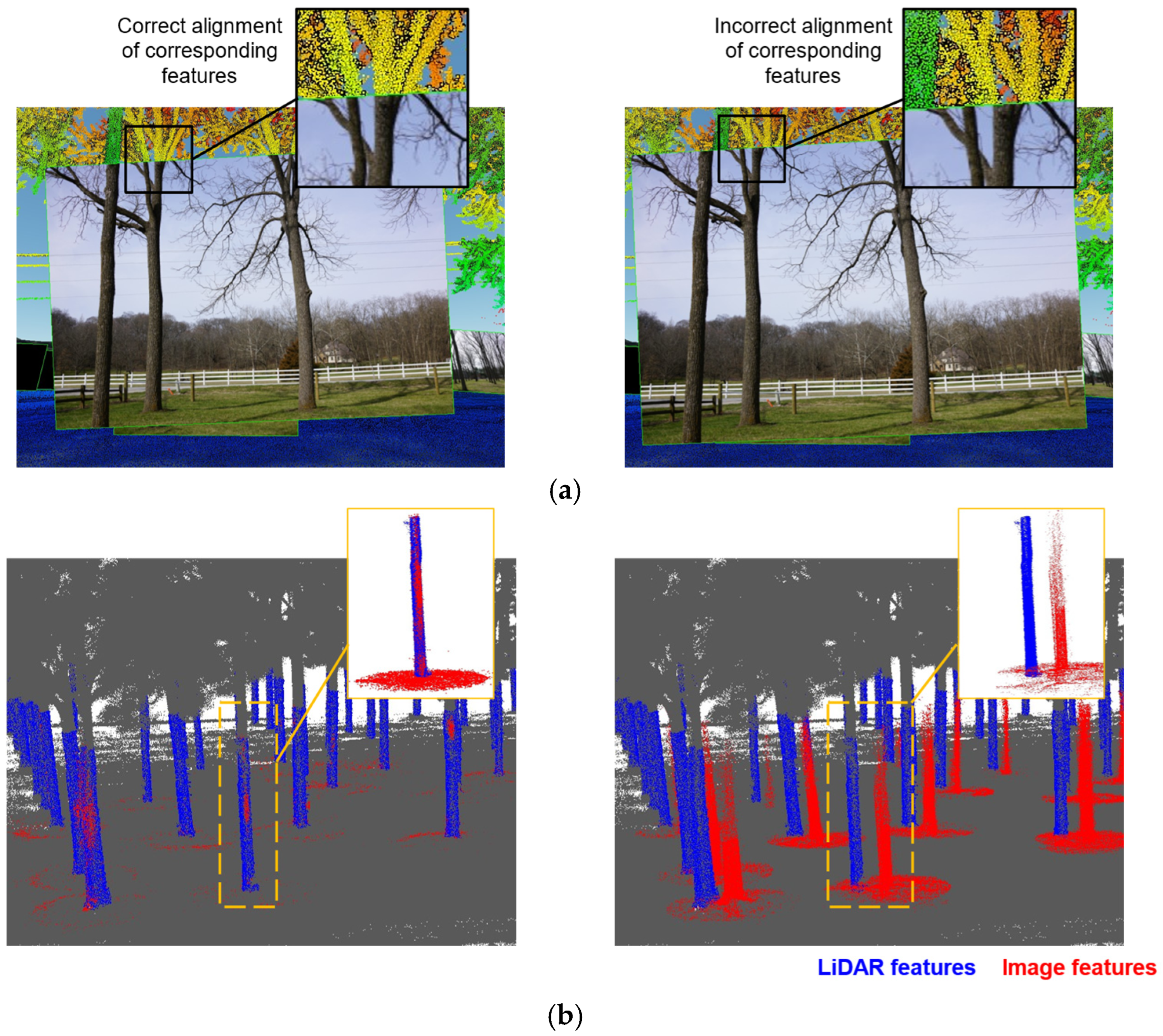
Collectively, these factors affect the quality of the final geospatial products. Figure 1 presents examples of LiDAR point clouds and RGB images, rendered together using an online visualization tool [16]. These illustrations are generated taking into account the MMS trajectory and individual sensors’ mounting parameters (the georeferencing mechanism of a GNSS/INS-based Backpack system is detailed in Appendix A). As shown in Figure 1a,b, inaccuracies in calibration and/or trajectory can lead to misalignment of corresponding features between image and LiDAR data. In light of these challenges, this study proposes a Backpack-based hardware–software framework aimed at reducing disparities in sensor acquisition rates and improving georeferencing accuracy, whether affected by calibration drifts, GNSS outage, or differences in post-processing. The proposed approach leverages the complementary strengths of the sensors and environmental context to enhance system calibration and platform trajectory, as demonstrated through multiple field experiments.

2. Related Work

The ever-increasing interest in proximal mapping applications has fueled the emergence of various commercial and research-oriented LiDAR/camera systems [17,18,19,20,21,22]. Although proximal mapping in forestry is still evolving, several studies have used these platforms for various analyses of forest features [23,24,25,26,27]. The payloads on these systems consist of one or more cameras and laser scanners, which are either georeferenced using a GNSS/INS unit or coregistered to a local reference frame. Despite all the advancements, efforts to enhance imaging and laser scanning capabilities have remained largely uneven. As such, most proximal MMS have limitations, especially with respect to RGB cameras. Some of the limitations include limited resolution of still cameras at higher frame rates, unproven time-stamping accuracy for video cameras, cameras without global shutters, and, most importantly, the inflexibility of swapping/upgrading sensors. Furthermore, these platforms offer little opportunity for system recalibration without manufacturer support and an openly accessible architecture. It is worth mentioning that some newer LiDAR sensors can detect passive RGB signals [28]. However, their spectral information content is generally limited. Aside from the platform, another challenge in forest mapping is the unreliable GNSS beneath the canopy, resulting in misalignment of image and LiDAR data. Georeferencing issues may also arise from imprecise system calibration or differences in post-processing approaches between sensors. In view of the above challenges, several studies have proposed methods to mitigate poor georeferencing by integrating multiple platforms (e.g., above- and under-canopy systems such as UAVs and backpack systems) and/or sensors through multi-modal feature-based calibration and trajectory refinement [29,30,31]. These techniques can be broadly classified as 2D–2D, 2D–3D, and 3D–3D registration approaches. It is worth mentioning that these broad classifications are applicable to both real-time adjustments (as in SLAM), or post-processed enhancements of image–LiDAR data.

2.1. 2D–2D Registration Approaches for Image–LiDAR Data Enhancement

The 2D–2D registration approach follows an optimization using images and 2D rasters of point clouds. Among a few notable techniques, 3D points from LiDAR are transformed into depth or intensity maps and used together with RGB images [32,33,34]. From these images, features such as lines and SIFT points are extracted, followed by establishing feature correspondences and performing camera pose estimation. For further pose refinement, researchers often implement bundle adjustment techniques. Some studies have also explored the use of mutual information (MI), such as luminance or object height, between camera and LiDAR-based images in a joint entropy minimization problem [35,36]. In general, MI-based approaches are tolerant to large misalignment and do not require explicitly defined features. However, these methods fail in the complete absence of shared information. Given the difference in scan rates between LiDAR and imagery—which is the case with proximal sensing using the Backpack system—it is likely that the two modalities do not maintain a correspondence across the entire study area.

2.2. 2D–3D Registration Approaches for Image–LiDAR Data Enhancement

The 2D–3D registration approach for data enhancement entails an optimization using 2D features from images and 3D features from a LiDAR point cloud. Several studies have proposed techniques to identify and use conjugate features from the two modalities [37,38,39,40,41,42,43]. Researchers have attempted extracting 2D–3D linear geometric primitives from building structures to conduct a linear feature-based camera–LiDAR relative pose estimation [37,39]. Hasheminasab et al. [38] proposed the idea of using linear geometry of agricultural field rows together with 3D linear features from point clouds to improve the georeferencing precision for orthophoto generation. Wang et al. [40] extracted 2D instances of light poles from images along with their conjugates in 3D point clouds and used them for refining the exterior orientation parameters (EOP) of the camera. Among other studies that investigated platform localization in forest environment, a common technique is to identify tree stems in images and point clouds, followed by implementing an optimization algorithm to reduce their reprojection errors and improve platform trajectory [44,45]. In general, the 2D–3D approach can work without overlapping images. However, extracting and matching features between 2D images and LiDAR point clouds is often complicated.

2.3. 3D–3D Registration Approaches for Image–LiDAR Data Enhancement

The 3D–3D registration-based data enhancement, as the name suggests, uses 3D point clouds from image and LiDAR data. This approach employs SfM and/or multi-view stereo (MVS) on a set of overlapping images to generate sparse 3D points, followed by identifying tie features across these image-based and LiDAR point clouds. The features are then used in a bundle adjustment that minimizes the distance between photogrammetric object points and their corresponding LiDAR features, all while solving for feature model parameters, mounting parameters, and/or trajectory poses. Studies have used SfM-based sparse points in conjunction with 3D LiDAR points for establishing conjugate planar patches [46,47,48]. Other studies adopted different feature types, such as semantic objects, but based on a similar principle of 3D–3D feature-based data enhancement [49,50,51]. Yang and Chen [52] implemented SfM to recover an initial set of camera EOP; then further refined the EOP by registering LiDAR and image-based point clouds using the iterative closest-point (ICP) algorithm. Although the 3D–3D approach requires image overlap as well as distinct features in the two modalities, it is more robust to outliers or false detection than the 2D–3D approach. Another advantage is the ease of finding conjugate features in 3D point clouds.
Almost none of the existing studies in forest mapping have sought to address image–LiDAR misalignments arising from calibration errors, post-processing limitations, or trajectory inaccuracies by taking advantage of 3D semantic objects within the rich geometry of forest environments. This can be attributed to two major factors: first, the limitations imposed by MMS hardware, i.e., inadequate overlap among camera images, and second, the complicated process of extracting and matching conjugate features across image and LiDAR data collected in forests of differing complexity. This study addresses these limitations through the following contributions:
  • Development of a Backpack MMS that integrates cameras with enhanced frame-rate capabilities, along with LiDAR and GNSS/INS units, to demonstrate the advantage of improving image overlap in terrestrial mapping;
  • An algorithmic implementation that integrates image-based and LiDAR point clouds using conjugate features to enhance LiDAR/camera system calibration and platform trajectory; and
  • Assessment of the impact of the proposed hardware–software implementation on tree biometrics derived for different forest types and complexities.
The remainder of the paper is structured as follows: Section 3 presents the development of Backpack MMS hardware and the proposed methodology on image–LiDAR integration for system calibration and trajectory enhancement; Section 4 contains experimental results that evaluate the proposed methodology and its impact on tree biometrics; Section 5 discusses the results, focusing on the quality of the derived features; and finally, Section 6 summarizes the contributions and recommendations for future work.

3. Materials and Methods

3.1. Backpack MMS Hardware Development

This study developed a Backpack MMS with hardware and system configuration essential to demonstrate the enhanced capabilities of imagery and LiDAR point clouds in forest mapping applications. The development included sensor selection, platform design, and system integration, as explained below.

3.1.1. Sensor Selection and MMS Layout

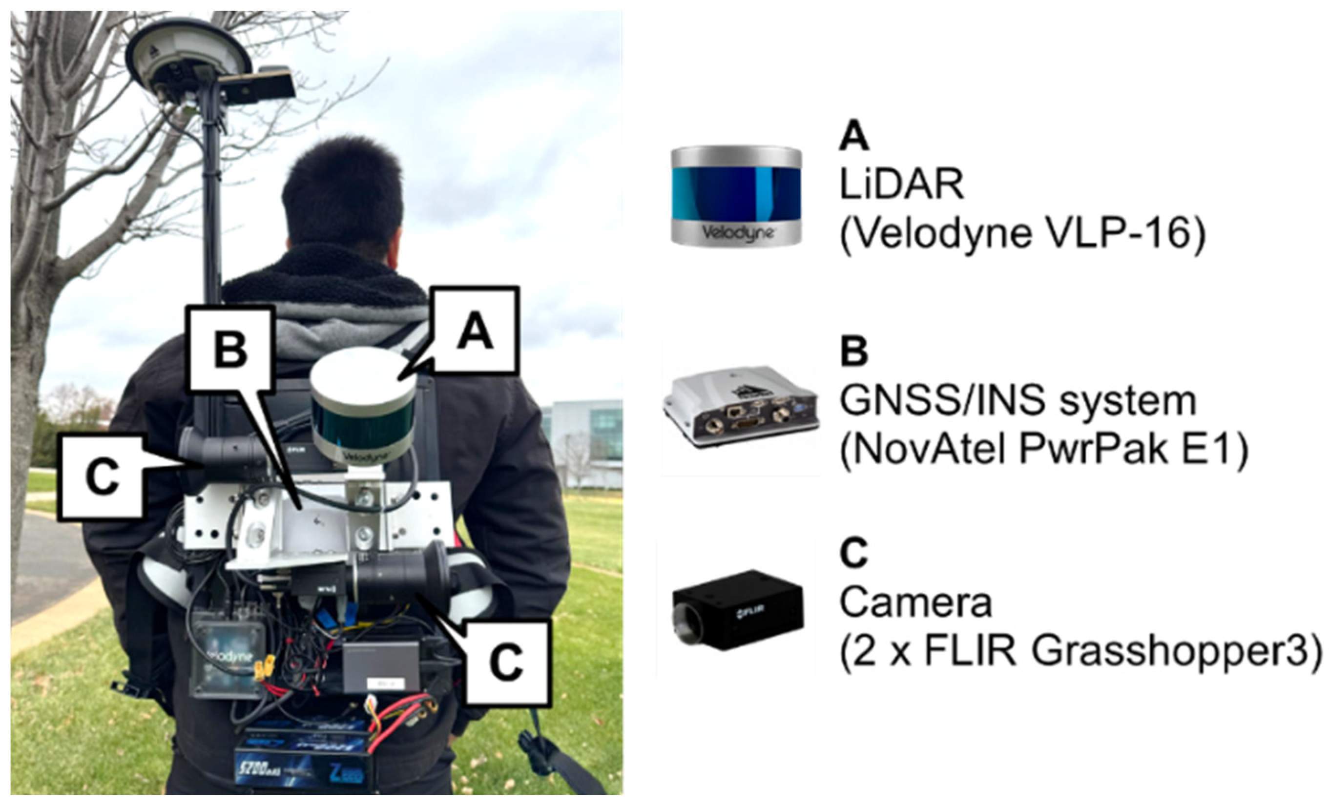
The Backpack development started with the selection and placement of sensors on the platform. Among several requirements, ensuring sufficient coverage and overlap among images required two cameras, each oriented toward one side of the Backpack. Furthermore, the cameras needed to have higher-than-standard frame rates (3–5 fps, compared to the typical 1 fps) and timestamps accurate to within a few microseconds. In addition, given the mobile nature of the platform, it was crucial for the camera to contain a global shutter. To address these needs, this study utilized two FLIR Grasshopper3 RGB frame cameras along with a NovAtel PwrPak7-E1 GNSS/INS unit and a Velodyne VLP-16 LiDAR on the platform [53,54,55]. The complete specifications of the RGB cameras, georeferencing unit, and LiDAR are listed in Table 1. The two Grasshopper3 frame cameras feature a 1” Sony CCD sensor and a global shutter mechanism. The NovAtel PwrPak7-E1 supports multiple satellite constellations (including GPS and GLONASS) for positioning and records raw GNSS/INS data, while concurrently logging camera events and time-stamping LiDAR measurements. The Velodyne VLP-16 is a multi-beam spinning LiDAR featuring 16 laser rangefinders arranged radially on a spindle, providing a vertical field-of-view (FOV) of 30 ° and a horizontal sweep of 360 ° . All these sensors are operated using a remotely controlled Raspberry Pi 4B computer, through which a user can control and monitor individual sensors and verify the acquired data in the field.
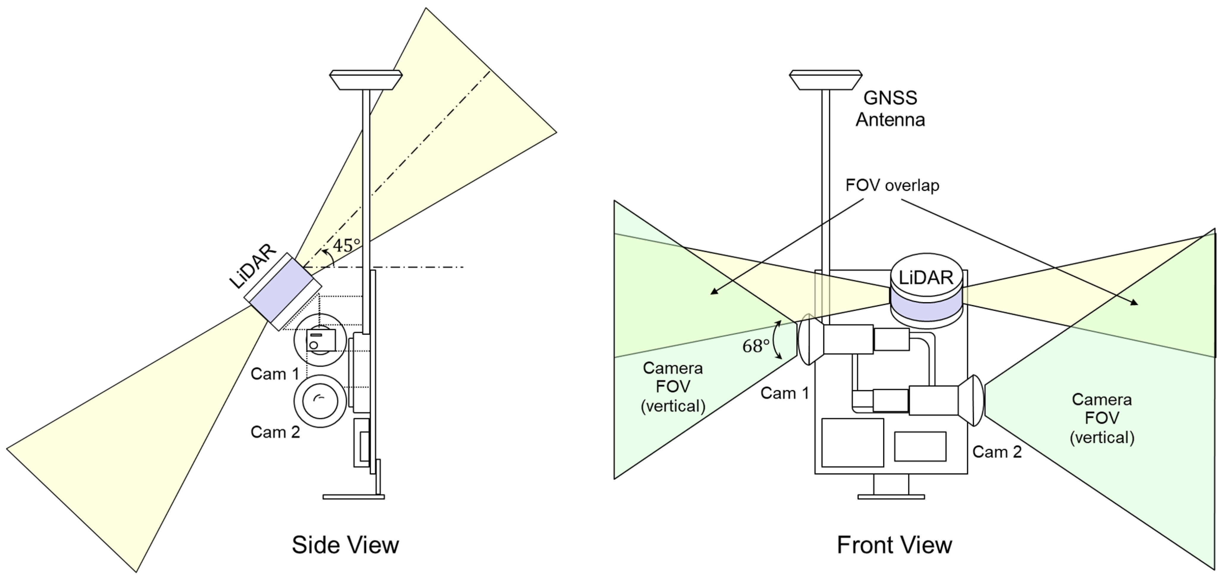
Figure 2 illustrates the layout of the system and the FOV of its LiDAR sensor and cameras. The presented layout ensures that the various sensors’ FOVs have a reasonable overlap, while minimizing any obstructions caused by the operator or other system components. The LiDAR is tilted at approximately 45 ° to simultaneously capture ground surfaces and objects located next to and above the operator. Depending on the motion and trajectory, the LiDAR point density within the forest varies across different regions. The two cameras are positioned to cover opposite sides of the platform: camera 1 is mounted upright facing the left, while camera 2 is installed inverted to capture the right side. Apart from the intended widening of the cameras’ FOVs, this setup was also influenced by the space constraint on the platform. Figure 3 shows the complete Backpack system based on the planned design. Each camera is configured to acquire images at 3 frames per second, which was found to be an optimal trade-off between the desired image overlap—assuming an average walking speed of 1.5 m/s—and the available data bandwidth. In addition, the cameras operate with a fixed exposure value (EV) of 1.5 and a shutter speed of 1/1000 s per frame, the latter being essential for minimizing motion blur. Throughout the operation, the camera’s automatic gain control handles variations in under-canopy lighting conditions.

3.1.2. System Integration

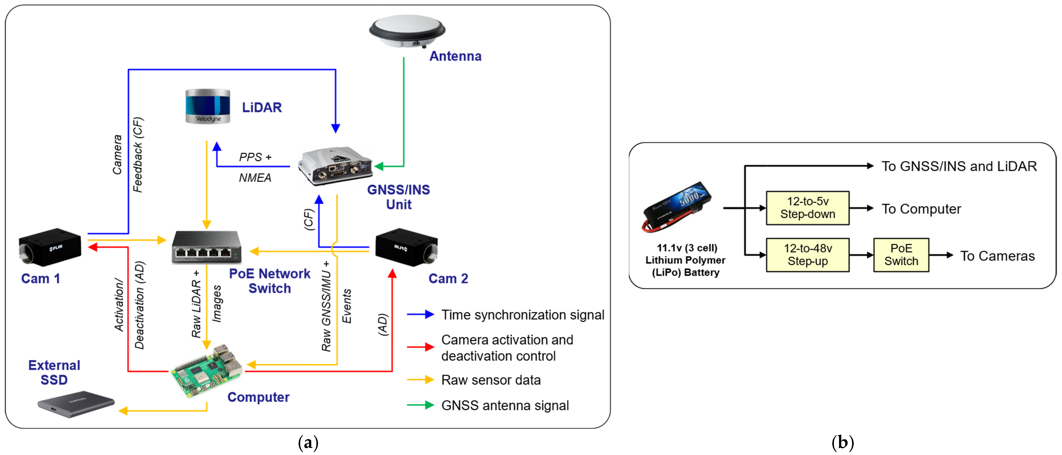
The prototyping stage also included planning efficient data logging and power distribution across the sensors. Figure 4 shows the data and power distribution schemes for the developed system (note that this figure depicts sensor connectivity only and does not necessarily represent actual physical wiring). Signals requiring different voltage levels and polarities, such as the GNSS antenna input, data transfer lines, and timing signals, are physically isolated from one another using separate cables. On the other hand, data packets from both the LiDAR and cameras, which share the same communication protocols, are routed through a common network switch to the computer. The switch also supplies power to the two cameras via Power-over-Ethernet (PoE). The power supply unit converts the source voltage to various levels as per the device’s requirements. The cameras are software-triggered over the Ethernet using manufacturer-provided libraries; once initiated, they continue capturing images at fixed intervals based on their internal settings. Simultaneously, a pulse corresponding to each exposure is transmitted to the event ports of the GNSS/INS unit through an external wire harness, enabling the cameras’ exposure times to be recorded with high precision alongside the raw GNSS/INS data. For LiDAR, timing signals received from the navigation unit, comprising pulse-per-second (PPS) and NMEA messages, are used for time-stamping individual returns. The approximate bandwidth consumed by the data logs (raw images and GNSS/INS data) arriving from all sensors to the computer is about 500 mbps and the run time of the system using two lithium-polymer (LiPo) 11.1V 5000mAh batteries is estimated to be around 1.5 h. All incoming data logs are stored on an externally connected solid-state drive (SSD).
Once the Backpack hardware was set up, the system was calibrated to determine the internal characteristics—i.e., interior orientation parameters (IOP)—and mounting parameters of LiDAR and cameras. LiDAR IOP are usually factory-calibrated and do not need refinement due to their stability. In contrast, camera IOP had to be estimated in situ, since these parameters are not stable and are unique for each camera. This study applied the self-calibration technique for IOP estimation introduced by Habib and Morgan [56]. As for the mounting parameters of the three sensors, they were obtained using the target-based system calibration procedure proposed by Radhika et al. [57]. The accuracy of the final ground coordinates was evaluated using the LiDAR error propagation calculator developed by Habib et al. [58]. For a sensor-to-object distance of 10 m, the accuracy is in the range of ± 2.5–3 cm.

3.2. Methodology for Camera/LiDAR System Calibration and Trajectory Enhancement

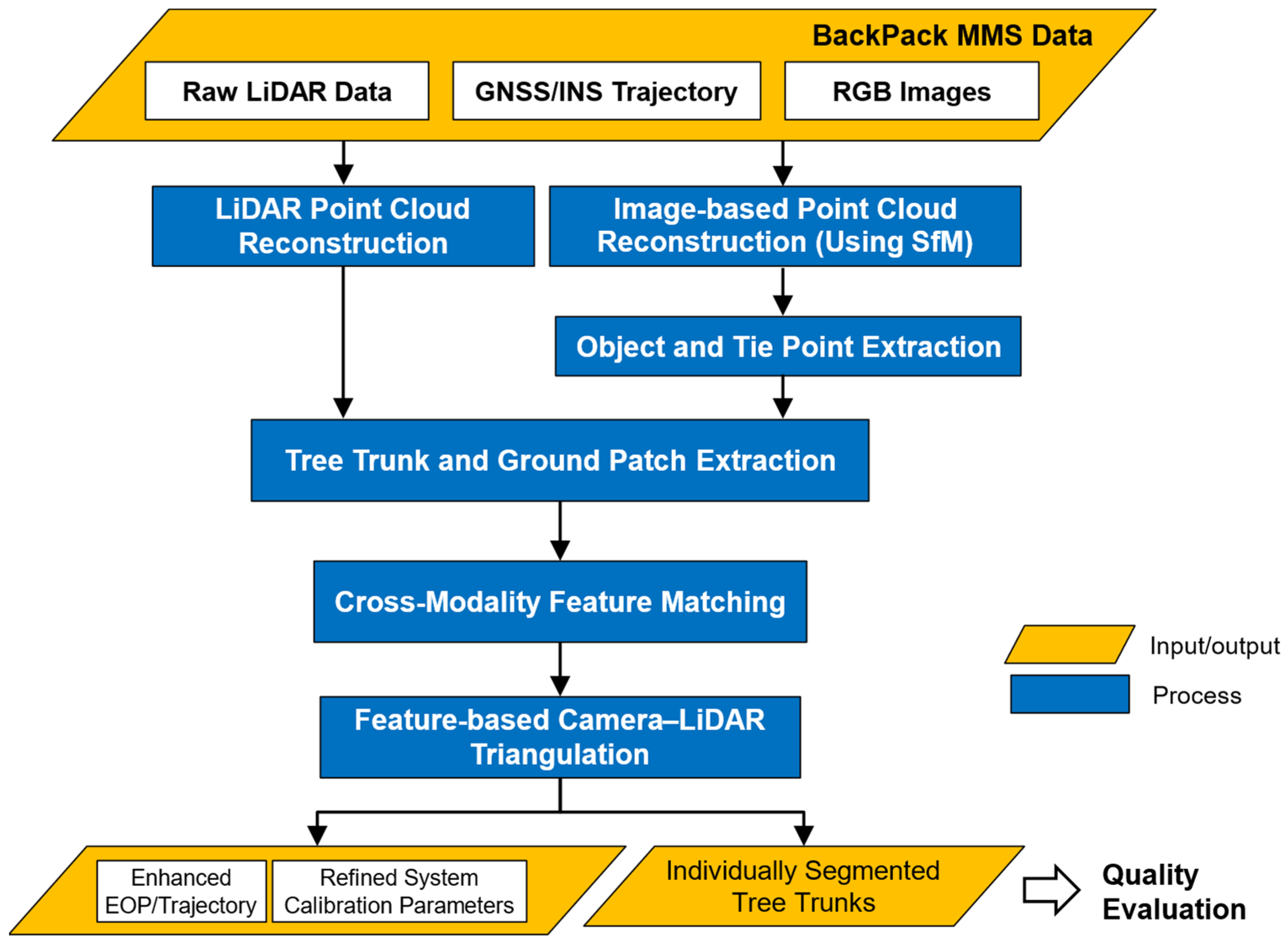
As previously mentioned, Backpack MMS often experiences GNSS outage under tree canopy. An important point to note is that outages do not occur only when the obstacles are overhead. Even a partial obstruction of the line of sight to satellites due to trees rising above the horizon can degrade the platform’s positional accuracy. Besides the GNSS outage, a less common but still well-known issue is the presence of a calibration bias, either as an artifact from the conventional calibration process or one that is introduced over the course of regular handling and operations. This section presents an in situ system calibration and trajectory enhancement approach for the newly built Backpack used for mapping forest environments. The approach is based on the hypothesis that forest point clouds have an abundance of tree trunks and ground surfaces. If these forest features could be identified and extracted as geometric primitives from each of the camera/LiDAR point clouds, one could define a set of target functions that optimize feature misalignments while refining the parameters sought after. Figure 5 outlines the workflow of the proposed approach, and the following subsections present the details of each step.

3.2.1. LiDAR and Image-Based Point Cloud Reconstruction

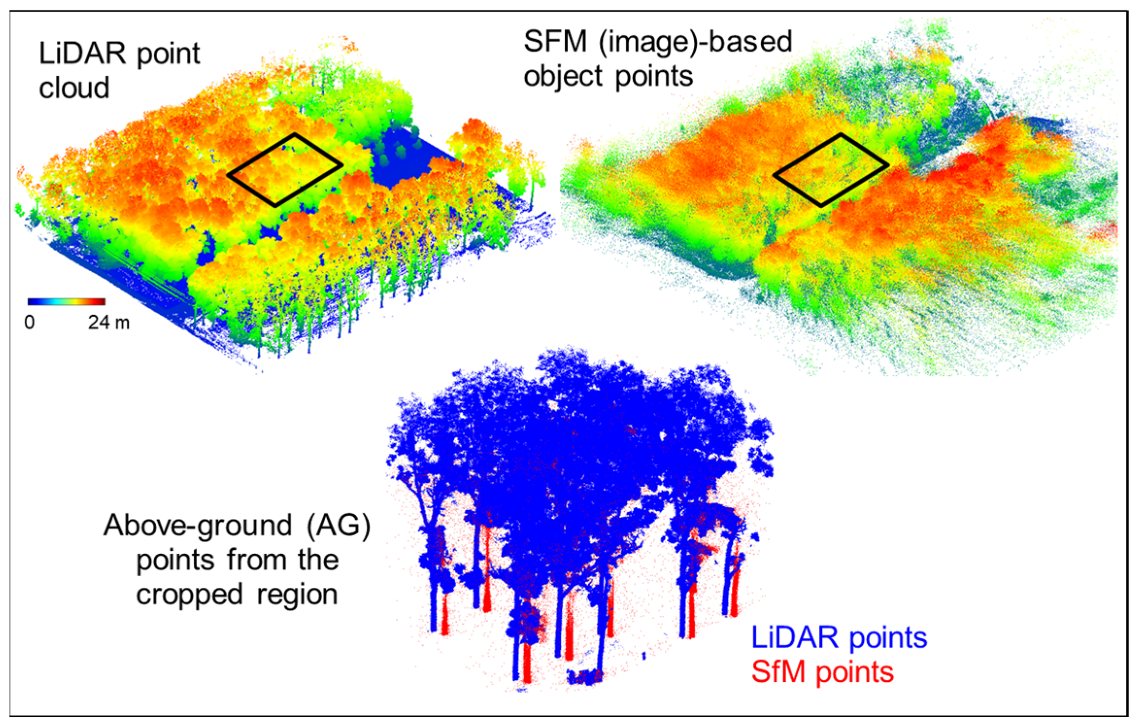
The proposed workflow is based on defining and extracting 3D primitives from LiDAR and imagery. As such, the first step entails generating LiDAR and image-based point clouds. LiDAR point clouds are obtained using a point cloud/trajectory optimization algorithm called Integrated Scan Simultaneous Trajectory Enhancement and Mapping (IS2-TEAM), developed for mapping in forest environments using Backpack LiDAR [29,59]. On the other hand, image-based point clouds are generated using structure-from-motion (SfM). Specifically, the SfM-based object points and their corresponding image points were obtained using Agisoft Metashape 2.2 [60]. The LiDAR and image-based point clouds, along with the camera IOP/EOP optimized by Metashape, serve as inputs for the proposed workflow in this study. Figure 6 shows sample LiDAR and image-based point clouds with a small section cropped from the two visualizing above-ground (AG) points and their levels of detail.

3.2.2. Tree Trunk and Ground Patch Extraction

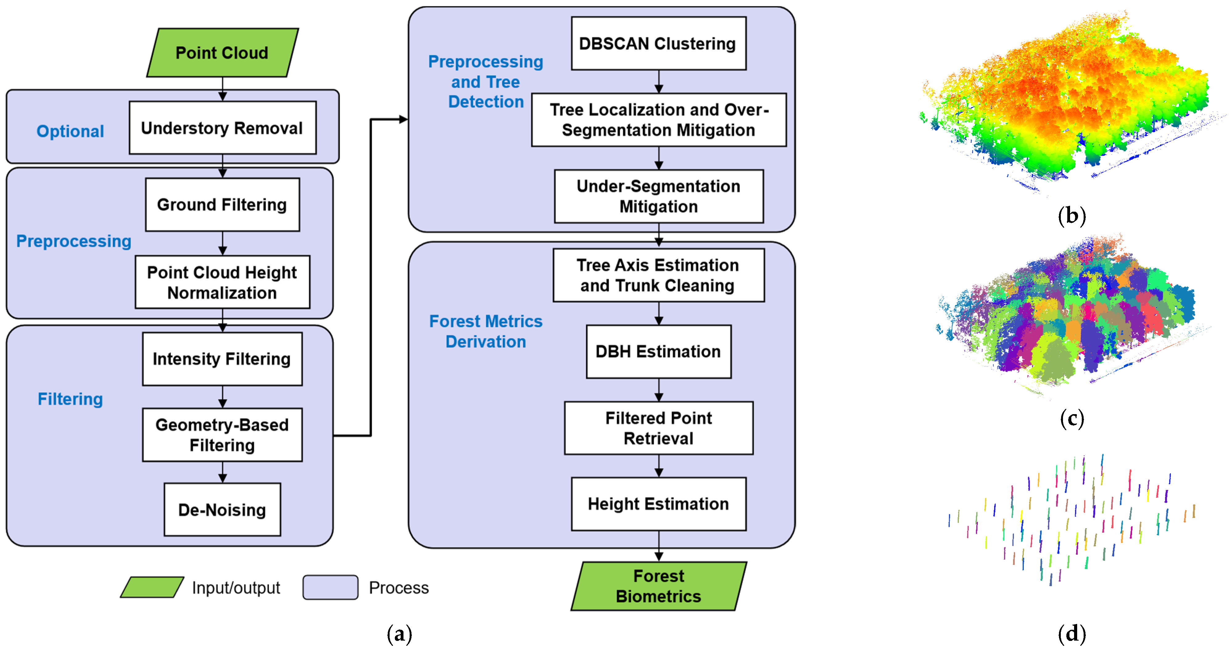
The proposed system calibration and trajectory enhancement approach relies on forest features that have well-defined geometries. This step implements a forestry pipeline to extract individual tree trunks from image/LiDAR point clouds [29]. Figure 7a outlines the pipeline, comprising preprocessing, filtering, tree detection, and forest metric derivation modules. The preprocessing stage includes a ground filtering algorithm to isolate AG points containing tree structures. This stage also includes a point cloud height normalization step, which enables data manipulation for individual tree segmentation, especially given the uneven nature of the terrain. Among the various filtering steps, the intensity-based filter uses LiDAR points’ intensity values to separate low- and high-intensity points, such as leaves from woody parts. A geometry-based filter identifies major woody parts based on their shape. After these filtering steps, any outlier points are then removed through de-noising by applying a statistical outlier removal (SOR) function. The above-mentioned filters are applied in different combinations depending on the nature of the forest environment. For instance, a natural forest may require multiple filters to remove any understory, which is usually non-existent in managed plantations. Subsequently, the tree detection module implements a clustering algorithm for segmenting individual trees, focusing on the cylindrical (i.e., lower) section of the trunk. The method works effectively on well-defined tree trunks, such as those in IS2-TEAM (LiDAR) point clouds. At the same time, one can adjust the clustering parameters to accommodate variations in the point cloud quality, as in the case of image-based points. Lastly, the forest metrics module estimates a variety of tree attributes, including trunk location, height, and diameter at breast height (DBH). Figure 7b–d show samples of the original point cloud, point cloud segmented into individual trees, and extracted tree trunks, respectively.
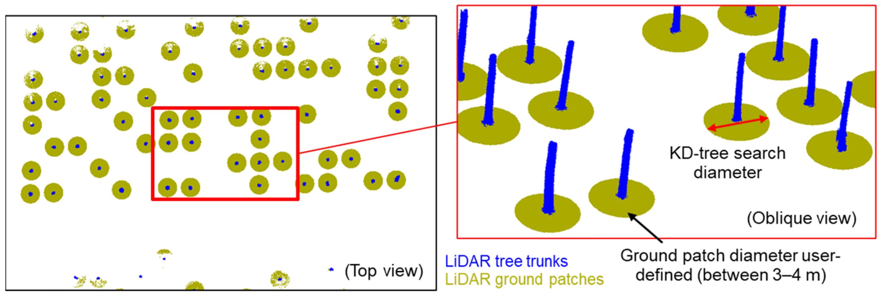
Once all the trunks have been isolated, an additional feature in the form of a ground patch is established for each individual trunk. These are defined around each trunk in the bare-earth (BE) point cloud as circular regions of a user-defined diameter (4 m in this study). Subsequently, the points within the demarcated region are extracted via a KDTree search [61]. Finally, these trunks and ground patches are modeled as geometric primitives—tree trunks as cylinders and ground patches as planes. While modeling tree trunks as cylinders does not fully represent their anatomical structure, this approximation has been widely adopted and consistently validated in prior studies on forest LiDAR datasets [9,62,63,64]. In practice, only a specific portion of the trunk—ranging from 0.5 m to 5 m in this study—is used for feature modeling, ensuring that only the most reliable segment contributes to the optimization. Moreover, successful optimization depends on a high degree of redundancy in both cylindrical and planar features. To meet this requirement, the proposed feature extraction process is fully automated, simplifying extraction by linking both feature types to each individual trunk. Thus, identifying conjugate trunk pairs between datasets implicitly establishes the matching ground patches as well. Figure 8 visualizes a sample set of tree trunks and ground patches based on the above approach.

3.2.3. Cross-Modality Feature Matching

Although both LiDAR and image-based point clouds are georeferenced, their alignment is not always ensured. This is due to the varying nature of SfM-based reconstruction, specifically the irregular distribution of matched features arising from non-uniform overlap of images, and separate processing of image blocks from the two cameras. Consequently, in addition to noise in individual features, conjugate features (tree trunks and ground patches) across the two modalities may not share identical spatial relationships (i.e., translational and rotational offsets) throughout the study area. This would influence the choice of method employed for matching features. In particular, methods that rely purely on Euclidean distance thresholds (here referred to as simple spatial proximity-based approaches) may fail to completely and correctly identify correspondences in different datasets. These approaches suffer from a lack of constraints and execute a greedy match simply based on the proximity rather than the structure of the neighborhood. To address such localized variations more effectively, this study introduces a global–structural approach to feature matching that integrates spatial proximity with the structural similarity of the neighborhoods. More specifically, the proposed method implements a global optimization that obtains all correspondences at once rather than an immediate match selection, as in the case of a simple proximity-based method. The approach formulates point correspondence as a linear assignment problem, using locally derived structural descriptors to achieve a simple, scalable, and computationally efficient method for establishing density-robust one-to-one matches. The matching is initially conducted only between trunk locations based on their 2D distances. However, as discussed earlier, identifying conjugate trunk pairs between image and LiDAR datasets implicitly identifies conjugate ground patch pairs, as the two feature types are intrinsically tied.
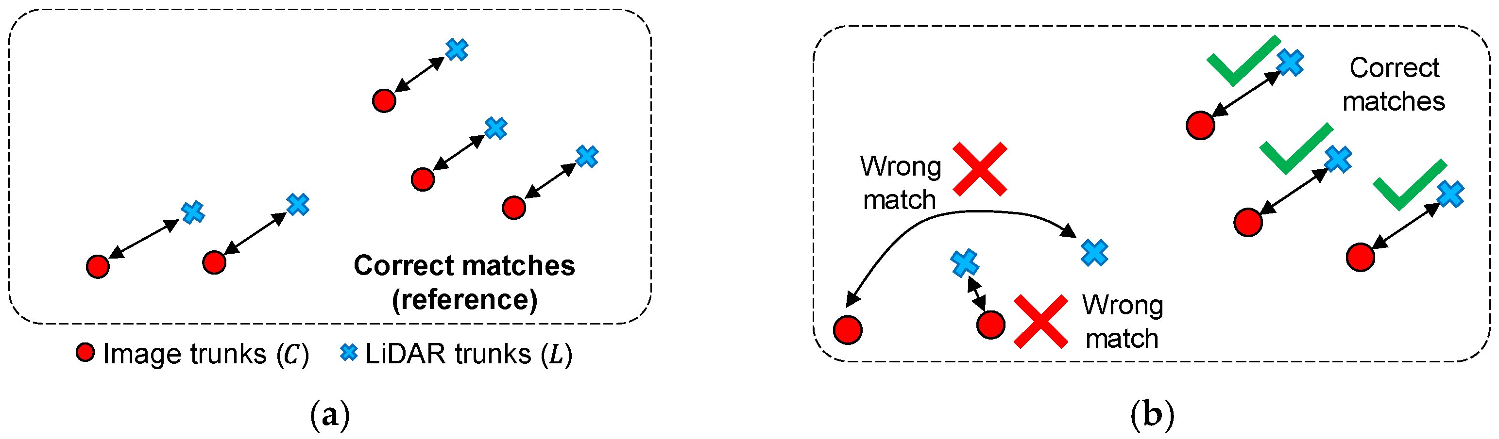
To illustrate the proposed feature matching strategy, suppose there are a total of m trunks in the image-based point cloud and n trunks in the LiDAR point cloud, and their correct matches are as shown in Figure 9a. Let C i and L j be, respectively, the i t h and j t h trunks in image and LiDAR datasets. Then, the planimetric Euclidean distance between the centers of two trunks is given by Equation (1). Next, let the pairwise match between element i and its corresponding match σ ( i ) be denoted by { i , σ ( i ) } , where σ I n j e c t i v e ( m , n ) , i.e., one-to-one mapping from the set of m elements to the set of n elements. Then, the simple spatial proximity-based match criterion, which is applied once for each C i , will be expressed as in Equation (2). The result of this matching approach is illustrated in Figure 9b. One can notice that a few features are incorrectly matched with their counterpart from the other dataset, which is expected from this method.
D   C i , L j = C i L j 2 for   i { 1,2 , , m } and   j { 1,2 , , n }
σ i = arg min σ Inj m , n C i L σ i 2      i { 1,2 , , m }
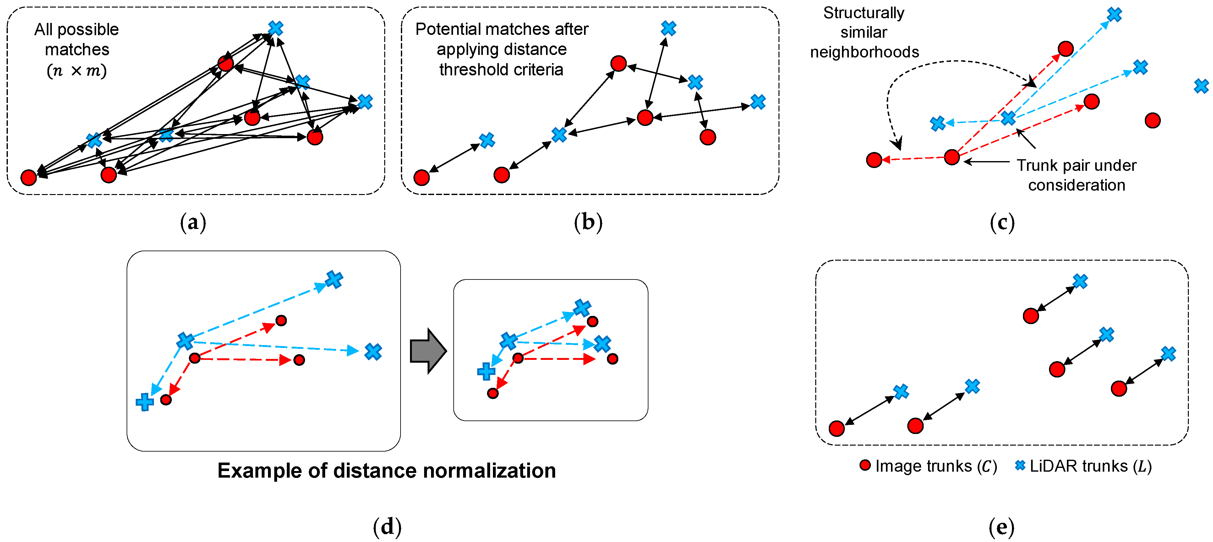
The proposed matching strategy starts with the same principle of spatial proximity. But unlike the limited constraint of the original search criterion, the proposed approach implements an expansive global–structural constrained cost function, comprising Euclidean distance between features across datasets and an additional metric defined by neighborhood structural similarity. The latter, as its name suggests, quantifies the similarity of feature arrangements within a localized region. The concept of neighborhood structural similarity is illustrated through Figure 10a–d. Initially, the complete set of potential match pairs across datasets is filtered down to those within a specified distance threshold, as shown by Figure 10a,b. This improves the efficiency of subsequent steps. Then, for each query trunk pair between image and LiDAR datasets, the procedure identifies K nearest neighboring trunks of the two candidates, with K set in the range 5–20 depending on the environment complexity, as shown in Figure 10c (three neighbors are shown for illustration). This is followed by computing the normalized distance D N between individual candidates and their neighbors. The normalization step compensates for pose discrepancies across datasets by scaling Euclidean distances to a range between 0 and 1. This ensures the neighborhood structures are comparable. Figure 10d illustrates the normalization process. Mathematically, for the trunks in the query pair { C i , L j }, their respective normalized distance arrays are given by Equations (3) and (4). Here, C i k and L j k are k t h nearest neighbors of C i and L j , respectively. Note that the process simultaneously performs array sorting.
{ D N C i , C i k   |   1 k K } = { D C i , C i k   |   1 k K } max 1 k K D C i , C i k = D N C i , C i 1 D N C i , C i 2 D N C i , C i K
{ D N L j , L j k   |   1 k K } = { D L j , L j k   |   1 k K } max 1 k K D L j , L j k = D N L j , L j 1 D N L j , L j 2 D N L j , L j K
Thereafter, a difference function is defined for each potential match pair to compute the Euclidean norm of pairwise discrepancies between corresponding normalized distances, as represented in Equation (5). This is the cost defined for the structural similarity criterion. In the ideal scenario of trajectories characterized by constant shift, this cost should be equal to zero for correctly matched pairs.
  • For each query pair { C i , L j },
D s t r u c t C i , L j = D N C i , C i k D N L j , L j k | 1 k K 2 = D N C i , C i 1 D N L j , L j 1 D N C i , C i 2 D N L j , L j 2 D N C i , C i K D N L j , L j K 2
The final optimization cost comprises a combination of spatial proximity and structural similarity components, as given by Equation (6). Here, the constants α and β are user-defined weights, empirically selected according to forest complexity and anticipated trajectory variations. In this study, the two weights are set to 2.5 and 0.8, respectively. These values imply that for the sites investigated, the spatial component played a larger role in ensuring correct matches in most areas. Subsequently, the minimization function for optimal feature matching is expressed as Equation (7). The solver used for this optimization is based on the Hungarian algorithm, widely known for its efficiency in solving linear assignment problems [65].
Total feature matching cost = α spatial cost + β structural cost
σ * { c o m b i n e d } = arg min σ Inj ( m , n ) i = 1 m α D i , σ i s p a t i a l + β D i , σ i ( s t r u c t u r a l )
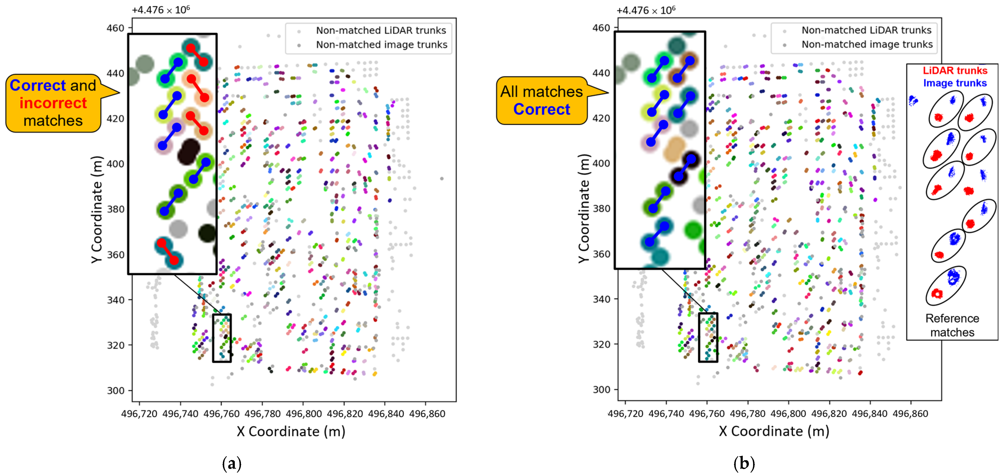
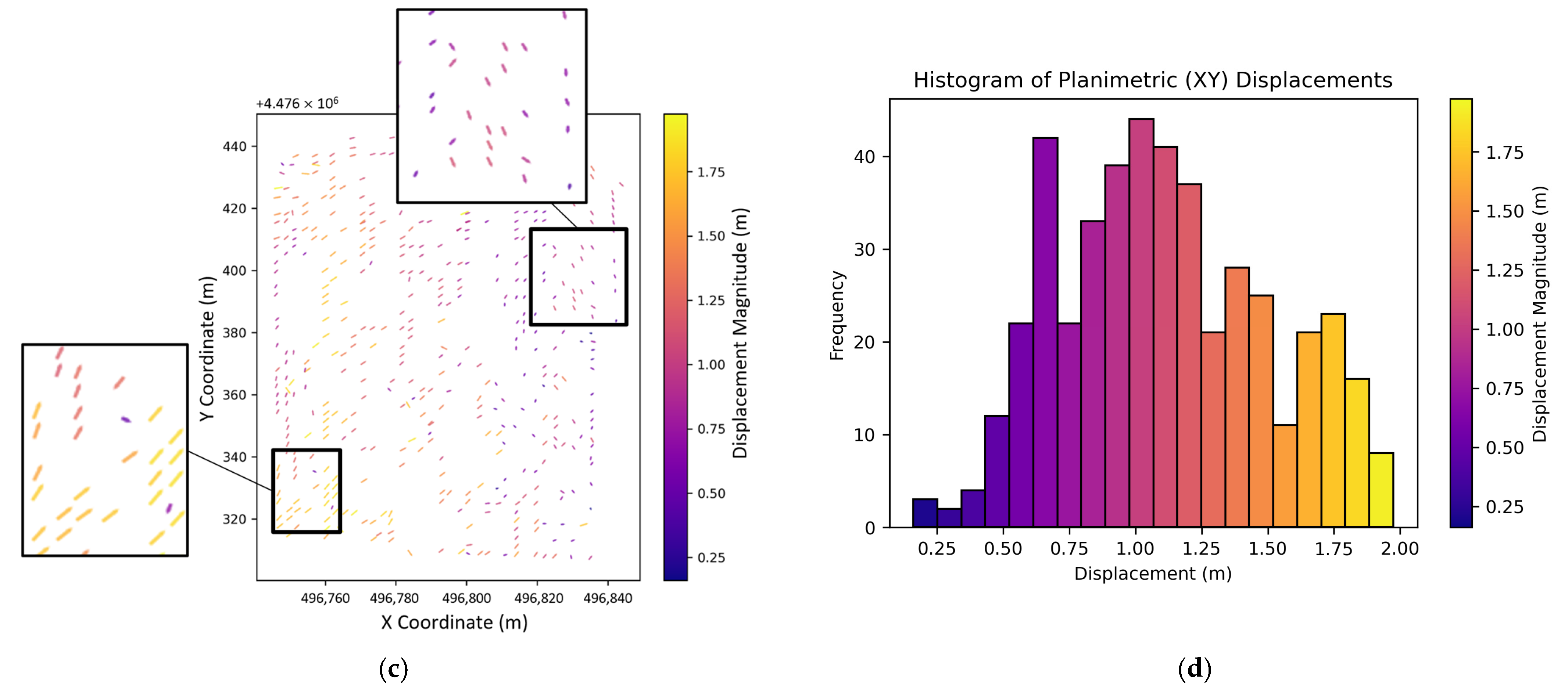
Figure 11 compares the results of the proposed method with those of the simple spatial proximity-based approach when applied to a forest image–LiDAR dataset. For this comparison, the reference matches were manually verified in the point clouds. One can observe that the latter approach results in several incorrect matches (Figure 11a), whereas the proposed method shows a promising result, i.e., it is more capable of handling variations in feature density and trajectory errors. Figure 11c and Figure 11d, respectively, visualize the planimetric offsets between conjugate features and their distribution, computed after the matching step. The varying nature of these displacements across the study site indicates the extent of discrepancies between the image and LiDAR trajectories.

3.2.4. Feature-Based LiDAR–Camera System Calibration and Trajectory Enhancement

This step involves applying all the plane–cylinder primitive pairs from the previous sections in a feature-based calibration/trajectory enhancement process, the final essential part of the methodology. The optimization algorithm developed in this study builds upon an earlier work on multi-sensor and multi-primitive triangulation, referred to as unified multi-sensor advanced triangulation (UMSAT) [66]. The framework supports a variety of sensors, such as LiDAR and frame/line cameras; trajectories from different platforms, like UAVs and backpacks; and diverse feature types, such as points, lines, and planes, and performs systematic adjustments capable of enhancing system calibration and trajectory while reconstructing optimized (LiDAR and image-based) point clouds. It is important to mention that the framework implements a system-driven approach for optimization, utilizing raw measurements (not the 3D points in mapping frame coordinates). The 3D point clouds are used primarily for extracting and matching features and are included in the adjustment only as initial approximations of the feature geometry. This study includes SfM-based 3D reconstruction along with LiDAR points to obtain planar/cylindrical feature pairs. Consequently, the UMSAT algorithm was augmented to accommodate cylindrical features derived from both LiDAR and image-based point clouds.
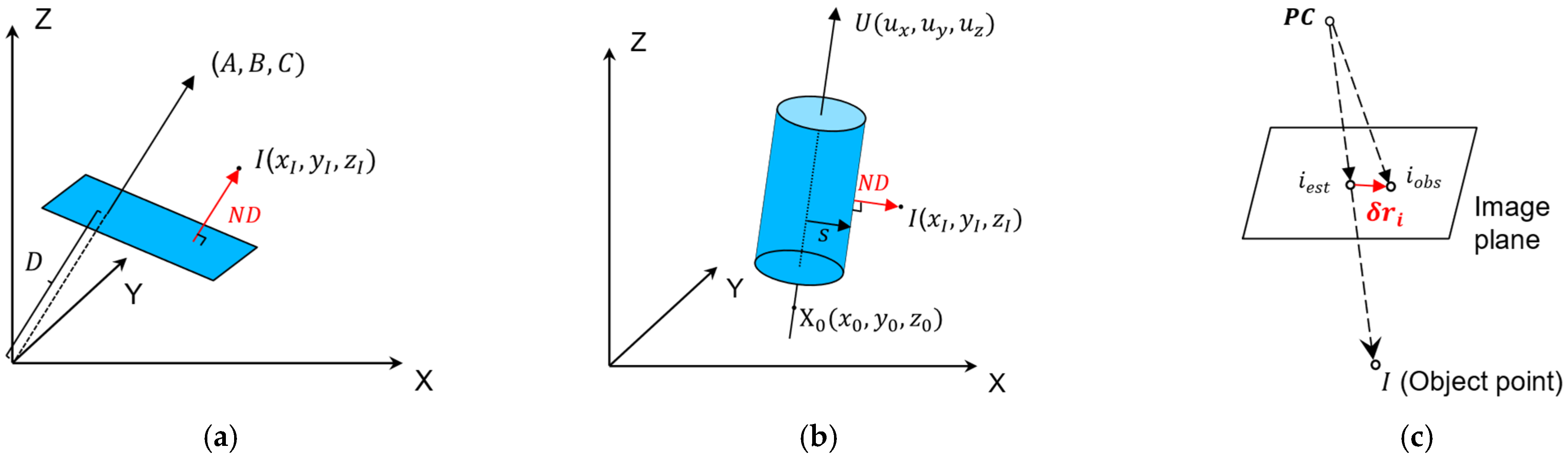
Conceptually, the solver behind UMSAT’s optimization engine performs least squares adjustment (LSA) using target/constraint functions for the available features. Considering the planar, cylindrical, and point features used in this study, the target functions for the LSA are established to minimize: (1) the sum of squared normal distances of object points (from LiDAR and image-based point clouds) to their corresponding planar/cylindrical features, and (2) the sum of squared back-projection errors of object points (from image-based point clouds) in the image plane. Figure 12 depicts the geometric interpretation of the minimization residuals, namely, the point-to-feature normal distance and back-projection error. Furthermore, their mathematical expressions have been outlined in Equations (8)–(10). If a planar feature is represented by the A ,   B ,   C ,   D plane parameters, then, for a feature point I denoted by ( x I , y I , z I ) , its normal distance to the plane is expressed by Equation (8). In the case of a cylindrical feature defined by the direction vector U ( u x , u y , u z ) , axial point X 0 ( x 0 , y 0 , z 0 ) , and radius s , the normal distance of a feature point I to the cylinder is given by Equation (9). Accordingly, the residuals corresponding to the planar and cylindrical features from LiDAR are functions of the feature parameters, LiDAR mounting parameters, platform trajectory, and LiDAR measurements comprising range ( ρ ) and direction ( d ), as expressed by Equation (10).
On the other hand, the image-based points are included in normal distance calculation under the constraint that they must coincide with defined planar and cylindrical features. Here, only the feature parameters and object points are updated while minimizing back-projection errors, according to Equations (11)–(13). In Equation (12), the back-projection error, δ r i c j , associated with camera j , is defined as the displacement between the observed image coordinates at i o b s (i.e., r i o b s c j ) and the projection of the corresponding object point I in image-based point cloud on the image plane at i e s t (i.e., r i e s t c j ). Equivalently, the back-projection residuals are functions of the mounting parameters, object point coordinates r I m , camera IOP, and observed image coordinates of camera j , together with the platform trajectory, as shown by Equation (13). The underlined parameters in Equations (10) and (13) represent non-estimated parameters, including observations expressed in their respective sensor coordinate frames, and camera IOP. It is worth noting that, unlike cameras, LiDAR does not involve unknown object points. As for the features, the LSA only adjusts parameters that are independent—planes and cylinders, respectively, have only three and five independent parameters. To summarize, UMSAT can include an object point in multiple target functions depending on its association with a feature. Thus, an image-based object point that also belongs to a planar/cylindrical feature must follow the normal distance as well as back-projection constraints.
N D I p l a n e = A x I + B y I + C z I + D A 2 + B 2 + C 2
N D I c y l = I X 0 I X 0 U U 2 s
r e s N D ( L i D A R ) = f F e a t u r e   P a r a m ,   r l u   b ,   R l u   b , r b t m , R b t m , ρ , d _
r e s N D i m a g e = f ( F e a t u r e   P a r a m ,   r I m )
r e s B a c k p r o j , δ r i c j = r i o b s c j r i e s t c j
r e s B a c k p r o j , δ r i c j = f r c j b , R c j b , r b t m , R b t m , r I m ,   c a m e r a IOP ,   r i o b s c j _
For this study, the camera IOP are obtained from the SfM result. As for the initial EOP of the cameras, they could also be obtained from SfM. However, because the GNSS/INS trajectory has already been optimized by IS2-TEAM, the initial EOP are derived from the IS2-TEAM trajectory. Using all available features and constraints, the LSA simultaneously optimizes feature model parameters, 3D point coordinates of image-based features, and system calibration/trajectory parameters. Equations (14) and (15), respectively, represent LiDAR and image point positions after the corrections. Here, c j refers to camera j , δ r b t m and δ R b t m are corrections to trajectory parameters, and r l u b r e f i n e d ,   R l u   b r e f i n e d and r c j b r e f i n e d ,   R c j   b r e f i n e d are corrected mounting parameters for LiDAR and camera, respectively. In general, system calibration and trajectory enhancement are performed separately to avoid any parameter correlations. Depending on the experimental objectives, the usual approach is to first refine the mounting parameters while fixing the trajectory, followed by trajectory adjustment while fixing the newly refined mounting parameters.
r I m t L i D A R , c o r r e c t e d = f r b t m , δ r b t m , R b t m , δ R b t m , r l u   b r e f i n e d ,   R l u   b r e f i n e d , r I l u t
r I m t c a m e r a , c o r r e c t e d = f r b t m , δ r b t m , R b t m , δ R b t m , r c j   b r e f i n e d ,   R c j   b r e f i n e d , r i c j ( t )
The trajectory enhancement procedure also involves a few additional preparations. Given that a trajectory comprises a large number of pose parameters, trajectory corrections are not solved for each LiDAR/camera observation, as it may lead to over-parameterization in the LSA. Instead, based on the platform dynamics, the trajectory is down-sampled at a user-defined time interval Δ T to establish trajectory reference points, as illustrated in Figure 13. Since the Backpack experiences moderate dynamics, the down-sampling rate is set to 5–10 Hz. During LSA, corrections to trajectory parameters at a given timestamp, say T 0 , are modeled as a function of n neighboring trajectory reference points. Notably, for cameras, the moment of the camera trigger or the image observation time itself is defined as a reference point.
The LSA for trajectory enhancement follows a set of equations that minimize: the point-to-parametric model normal distance, back-projection errors in the image plane, change in trajectory pose parameters (i.e., position and attitude), and change in distance between trajectory reference points, as given by Equations (16)–(19), respectively. In these equations, P a r a m ( k ) refers to the parameters of k t h feature, and δ θ b t i m denotes change in trajectory position ( δ r b t i m ) and orientation parameters ( δ R b t i m ) at reference point i . The expression in Equation (19) minimizes the change in distance traversed between two consecutive trajectory reference points. Here, the minimizing arguments δ r b t i m and δ r b t i + 1 m refer to changes in successive trajectory positions, respectively, at reference points i and i + 1 . The expression in Equation (19) ensures that the change in distance traversed between successive trajectory reference points is minimized, with changes only as necessary, to constrain the velocity. The terms w 1 , w 2 , w 3 and w 4 are, respectively, weights associated with normal distance, back-projection error, absolute trajectory accuracy, and relative or velocity accuracy. The weights are determined based on the a priori variances of the corresponding parameters, where lower variance receives higher weights, and vice versa. Accordingly, the weights are taken as the inverses of the a priori variances, which are based on available information from image/LiDAR feature points and GNSS/INS post-processing. In this study, the a priori variances for normal distance and image coordinate measurements are specified as 5   c m 2 and 7   p i x e l 2 , respectively. For corrections applied to trajectory reference points, the a priori variances of absolute changes in position and orientation parameters are set to 5   cm 2 and 0.10 ° 2 , respectively. Regarding the relative changes between successive reference points, the a priori variances adopted for position and orientation parameters are 0.15   c m 2 and 0.05 ° 2 , respectively.
arg min δ θ b ( t ) m , Param ( k ) I k w 1 N D k I k 2  
arg min δ θ b ( t ) m i , j w 2 δ r i c j 2
arg min δ θ b t i m i = 1 n w 3 δ θ b t i m 2
arg min δ r b t i m , δ r b t i + 1 m i = 1 n 1 w 4 D i ( c o r r e c t e d ) r b t i m , δ r b t i m , r b t i + 1 m , δ r b t i + 1 m D i r b t i m , r b t i + 1 m 2

4. Experiments

Several experiments were conducted across multiple study sites to demonstrate the proposed methodology for system calibration and trajectory enhancement. The experiments include system calibration of both Backpack cameras to obtain their refined mounting parameters, followed by trajectory enhancement. Apart from that, this section also evaluates the result based on LiDAR–camera back-projection and tree biometric estimates (location and DBH). Note that this study assumes the LiDAR system to be properly calibrated, i.e., its IOP and mounting parameters are precisely known, and that any residual calibration errors have likely been compensated for by IS2-TEAM. Nonetheless, the methodology presented for camera system calibration can also apply to the LiDAR units, if needed. The experiments report qualitative and quantitative results for calibration and trajectory enhancement, where applicable. The evaluation metrics include discrepancies between corresponding image–LiDAR features, back-projection residuals, and point-to-feature normal distances before and after optimization. In addition, the DBH estimates are also compared across datasets and with reference data.

4.1. Description of the Acquired Datasets

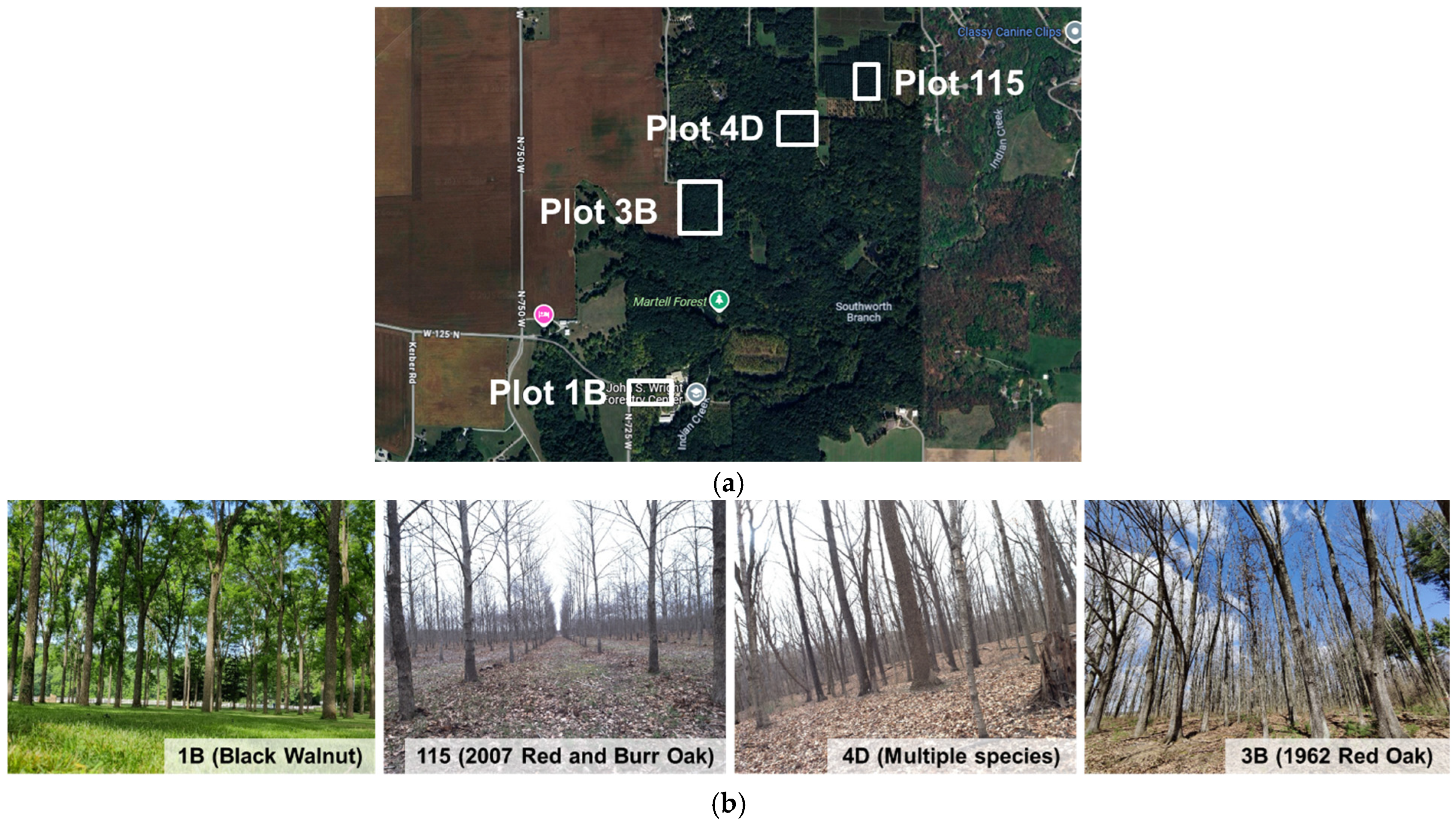
The experimental datasets comprise four study sites of various forest types and leaf-cover conditions—from plantation to natural, and leaf-on to leaf-off. Table 2 summarizes the details of these Backpack image–LiDAR datasets, including tree species, mission duration, number of LiDAR points, and number of captured RGB images. These sites are located within the Martell Forest area, Purdue University, IN, USA, as depicted in Figure 14a. Figure 14b shows the site conditions at the time of data collection—three out of the four datasets are from the leaf-off season.
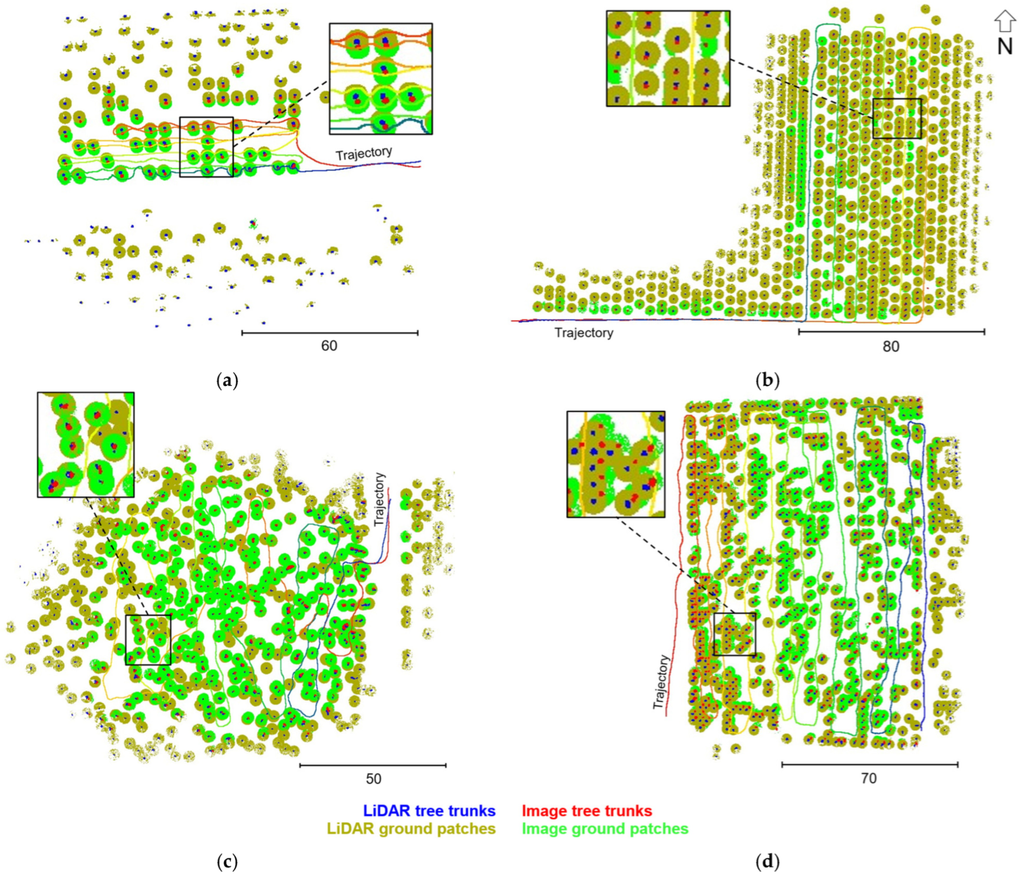
The image–LiDAR features together with the original GNSS/INS trajectory for all four datasets are shown in Figure 15. In addition, Table 3 summarizes the details of the extracted features—image measurements, corresponding tie points, and LiDAR points. From the figures and table, one can notice the high redundancy of feature points in both modalities, crucial for a reliable optimization.

4.2. Result of the Proposed System Calibration and Trajectory Enhancement

Using the four datasets presented above, the following experiments were conducted:
  • Experiment 1: LiDAR-assisted camera system calibration (dataset A)
  • Experiments 2–5: post-calibration trajectory enhancement (datasets A, B, C, D)
The idea behind two separate sets of experiments is that once the camera mounting parameters have been estimated, they need not be refined for later datasets collected within the same year. Regardless of whether system calibration is performed on each dataset, all these experiments involve the same set of observations and unknowns. Specifically, the observations comprise 2D image coordinates and LiDAR measurements; the unknowns are the image-based object points, feature parameters, and mounting/trajectory parameters.

4.2.1. Experiment 1: LiDAR-Assisted Camera System Calibration for Dataset A

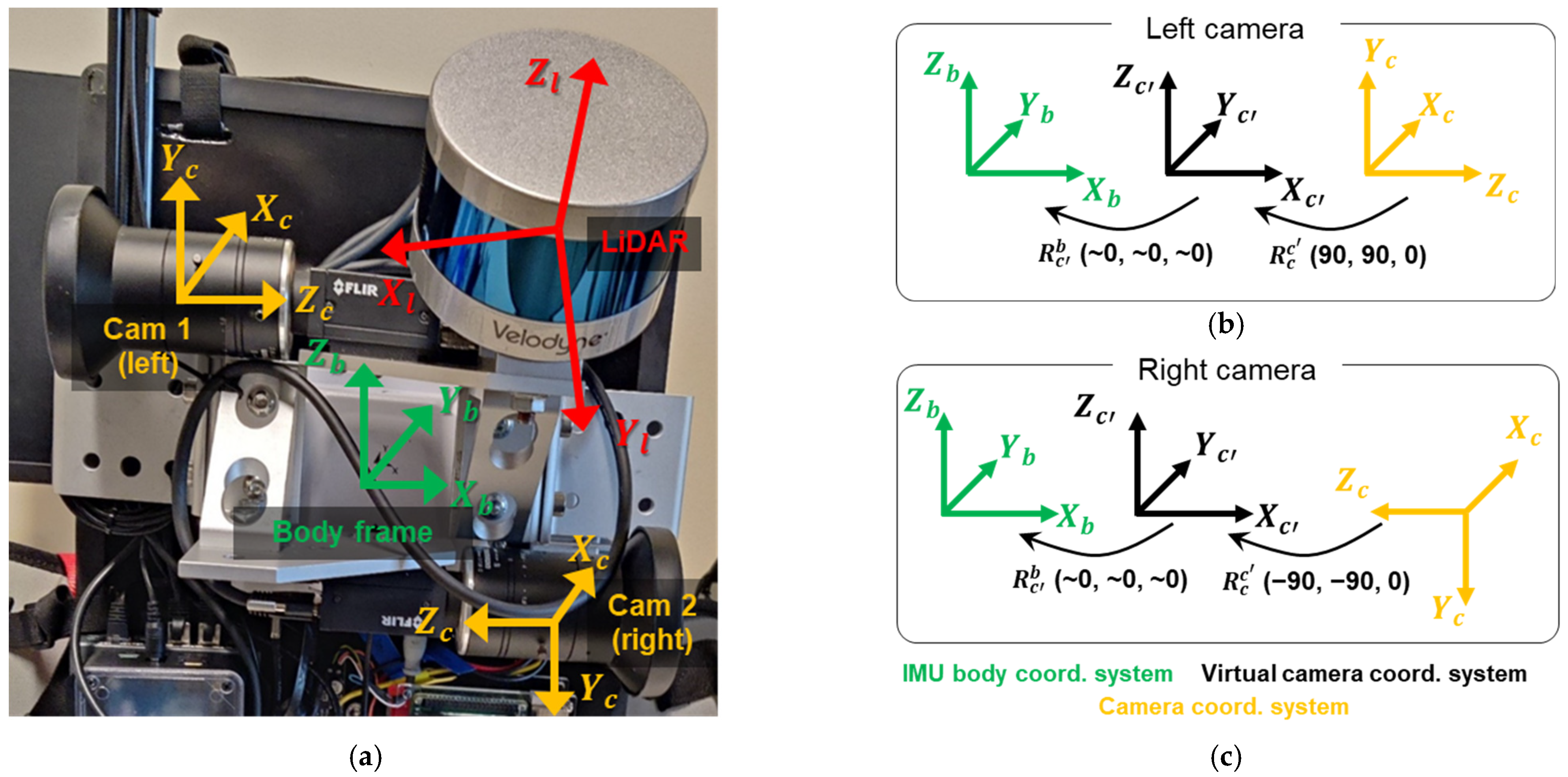
This experiment refines the mounting parameters of the two cameras while the trajectory is kept fixed. Figure 16a illustrates the coordinate frames of various sensors on the Backpack. The lever arm components and boresight angles between the IMU body frame and cameras are initialized with the prior calibration parameters. The boresight angles for the left and right cameras are roughly ( 90 ° , 90 ° , 0 ° ) and ( 90 ° , 90 ° , 0 ° ) , respectively. It is known that secondary rotations close to ± 90 ° would lead to gimbal lock issues. Hence, to avoid any unexpected outcome, UMSAT applies a fixed rotation equal to the nominal boresight of each camera to align the camera frame with the body frame (the new camera frame is henceforth termed as the virtual camera coordinate frame). This mitigates the gimbal lock issues as the calibration now only estimates the remaining incremental angular offsets between the virtual camera and body frames. Figure 16b,c demonstrate the rotation of the original camera frames to align with the body frame using the fixed rotation matrices, R c c . Accordingly, the estimated boresight angles define R c b .
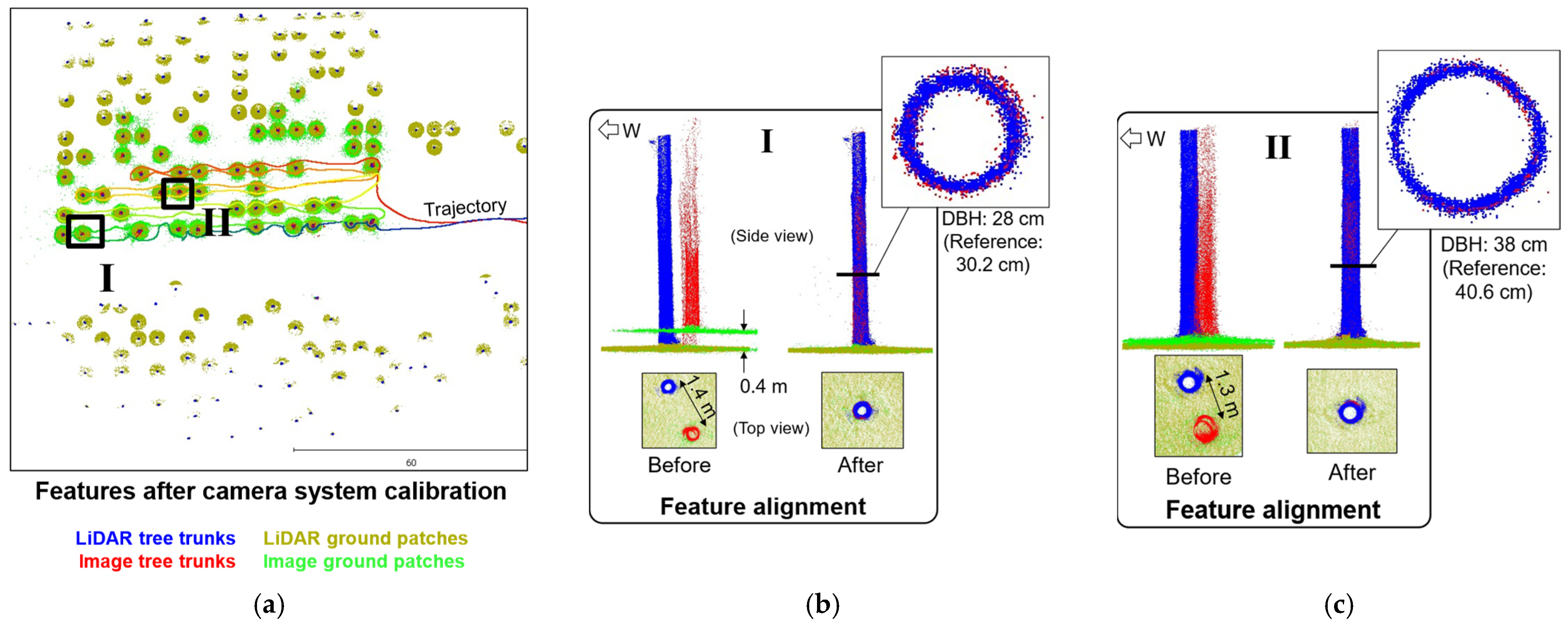
Table 4 reports the nominal and post-calibration mounting parameters—three lever arm and three boresight components, for each camera. One can notice that all six parameters were adjusted in both cameras. Figure 17 visualizes sample image–LiDAR point clouds before and after calibration. Additionally, Table 5 reports the planimetric and vertical discrepancies between the corresponding features. These values are based on 3D trunk locations computed in image and LiDAR datasets. Both qualitatively and quantitatively, the alignment of image–LiDAR features has substantially improved following the refinement. That said, some scattered points still exist around tree trunks, as seen in the callouts in Figure 17b,c.

4.2.2. Experiments 2–5: Post-Calibration Trajectory Enhancement

Following the system calibration, this second set of experiments performs an image–LiDAR feature-based trajectory optimization. It is important to recall that IS2-TEAM performs LiDAR-only optimization. The approach presented here incorporates an additional modality (camera) to improve the alignment of image and LiDAR point clouds while refining the platform trajectory. Thus, for trajectory enhancement, all four experimental datasets are included. In these experiments, the inputs comprise camera mounting parameters from the first experiment, LiDAR mounting parameters from prior calibration, and trajectory from IS2-TEAM. The mounting parameters are fixed, whereas the trajectory poses are adjusted according to the LSA constraints outlined in Section 3.2.4.
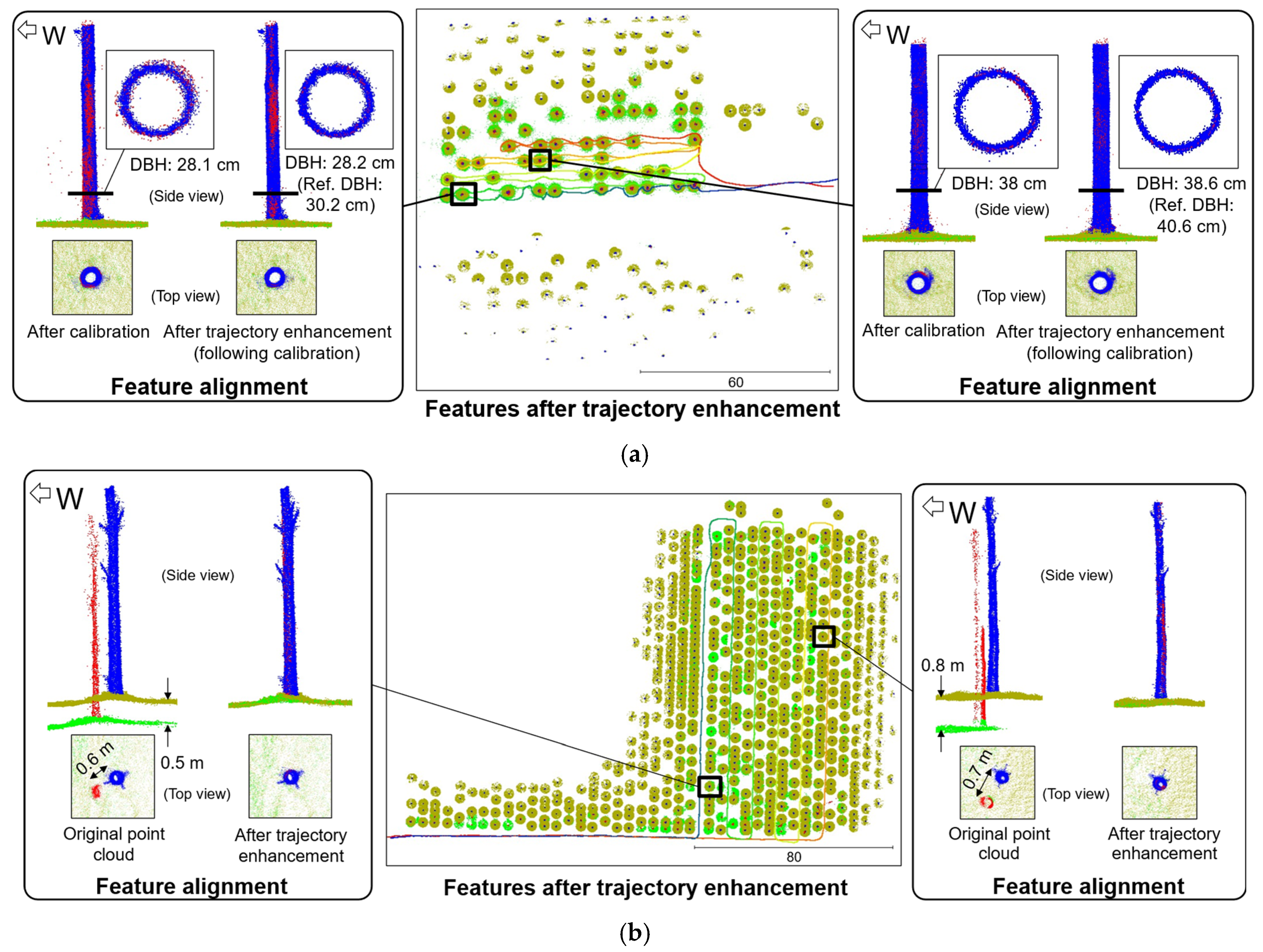
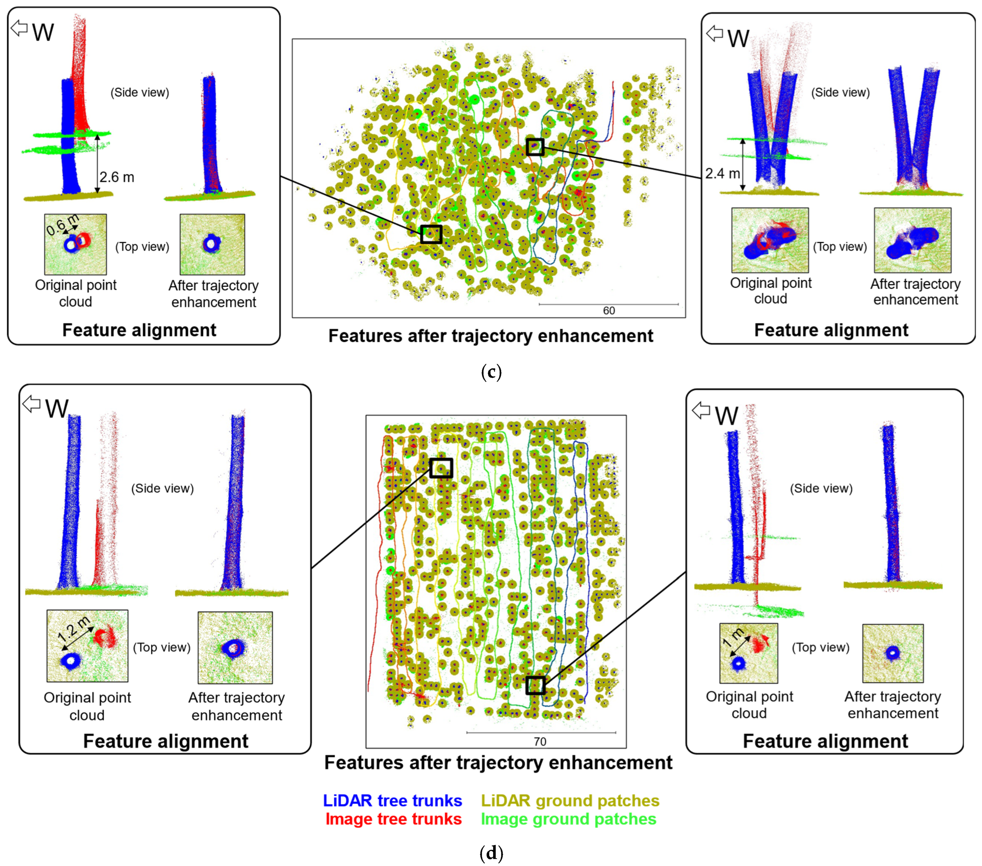
Figure 18 shows the alignment of features before and after trajectory/point cloud enhancement for all four experiments. Except for dataset A in Figure 18a, the changes in all other datasets are the combined outcome of calibration and trajectory refinement, i.e., these visualizations already include improvements from calibration. In Figure 18a, the callouts highlight the incremental improvement in feature quality only due to trajectory enhancement. Table 6 reports the quality metrics for dataset A, highlighting the additional change in feature quality between calibration and trajectory enhancement. For datasets B, C, and D, Table 7 enumerates the planimetric and vertical discrepancies between image and LiDAR features. Despite the large magnitudes of the initial misalignments in the three datasets, the proposed approach results in well-aligned features. In addition, features are less noisy and have well-defined profiles. From the trajectory’s perspective, its pose changes between the IS2-TEAM and UMSAT results are reported in Table 8 for each dataset. The adjustments shown in the table are consistent with the additional improvement observed in the point cloud, such as a reduction in scattered points, as shown in Figure 18a for dataset A.

4.3. Impact of the Proposed Approach on LiDAR–Camera Back-Projection

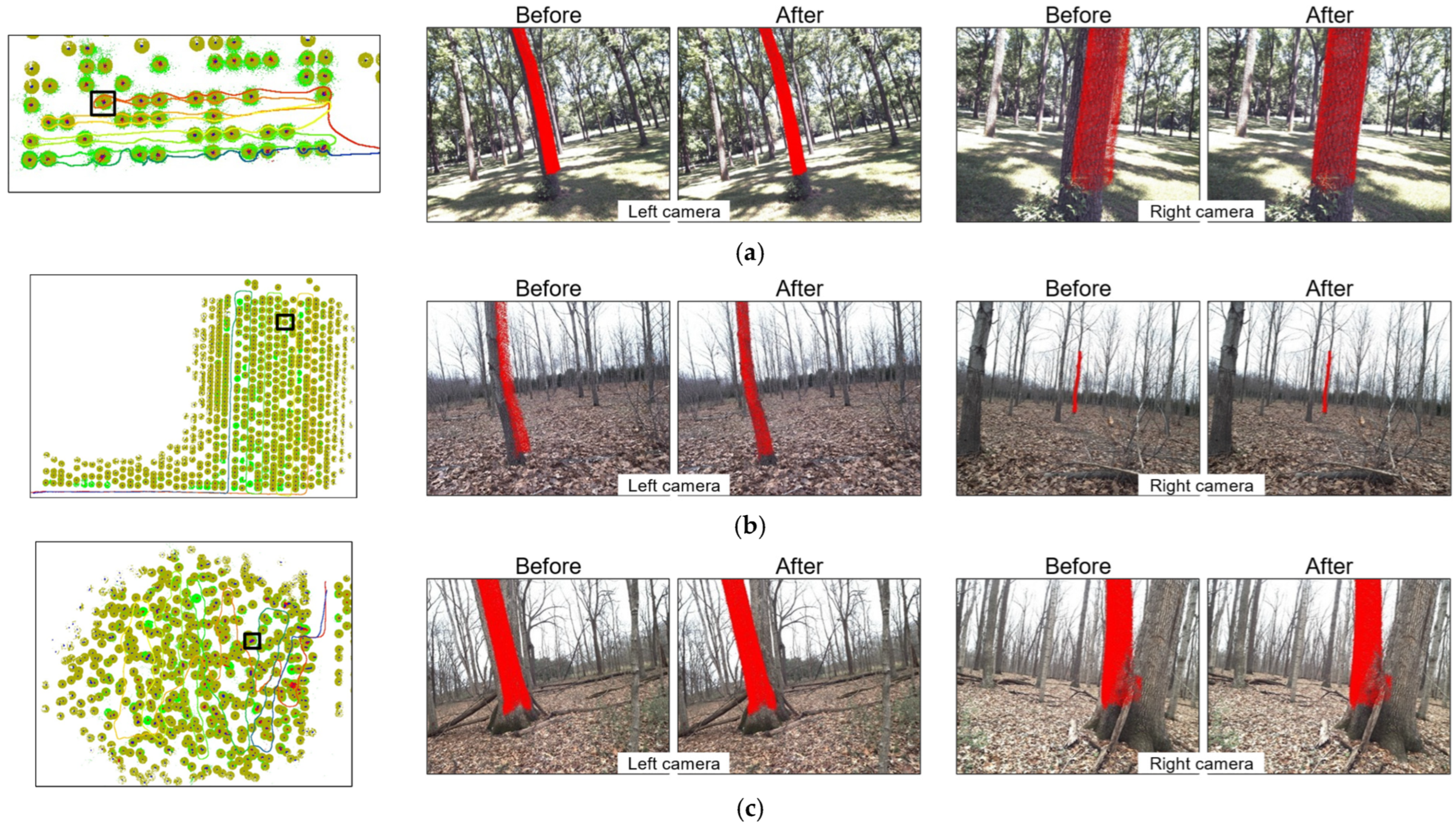
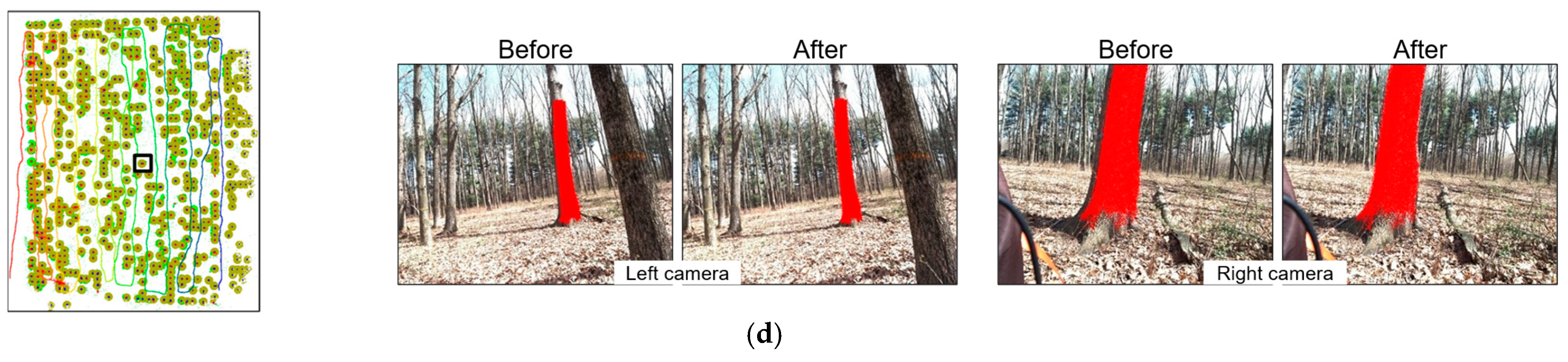
The quantitative and qualitative assessment of 3D point clouds presented before are effective ways to infer image–LiDAR data compatibility. However, for various practical applications, such as tree trunk segmentation for inventory and species ID, using 3D features may not be as convenient as 2D imagery. Therefore, along with assessing the alignment of multi-modal features in 3D, it is reasonable to evaluate image–LiDAR compatibility in 2D images. This is achieved by back-projecting LiDAR points onto images using the most recent calibration parameters and trajectory. Figure 19 visualizes the rendering of sample back-projections for various datasets before and after system calibration and trajectory enhancement. The trunk points shown in these figures are 0.5 m above the bare earth. The procedure results in a highly precise feature alignment, with the back-projection of 3D points accurately demarking trees in the imagery.

4.4. Impact of Image–LiDAR Data Enhancement on Tree Biometrics (DBH)

This section evaluates the proposed methodology based on DBH values derived from the enhanced point cloud. At the beginning, dataset A is investigated using four different optimization scenarios: (1) LiDAR-only optimization using IS2-TEAM, (2) LiDAR-only optimization using UMSAT following IS2-TEAM, (3) image-only optimization using UMSAT, and (4) combined image–LiDAR optimization using UMSAT following IS2-TEAM enhancement of LiDAR. These scenarios are useful for assessing the relative capability of the two modalities as well as of the two optimization algorithms. Dataset A also includes reference DBH values that were manually measured from a small subset of the site consisting of 42 trees. After dataset A, the subsequent evaluation of other datasets will only use the post-UMSAT calibration and trajectory enhancement results, as will be discussed later.
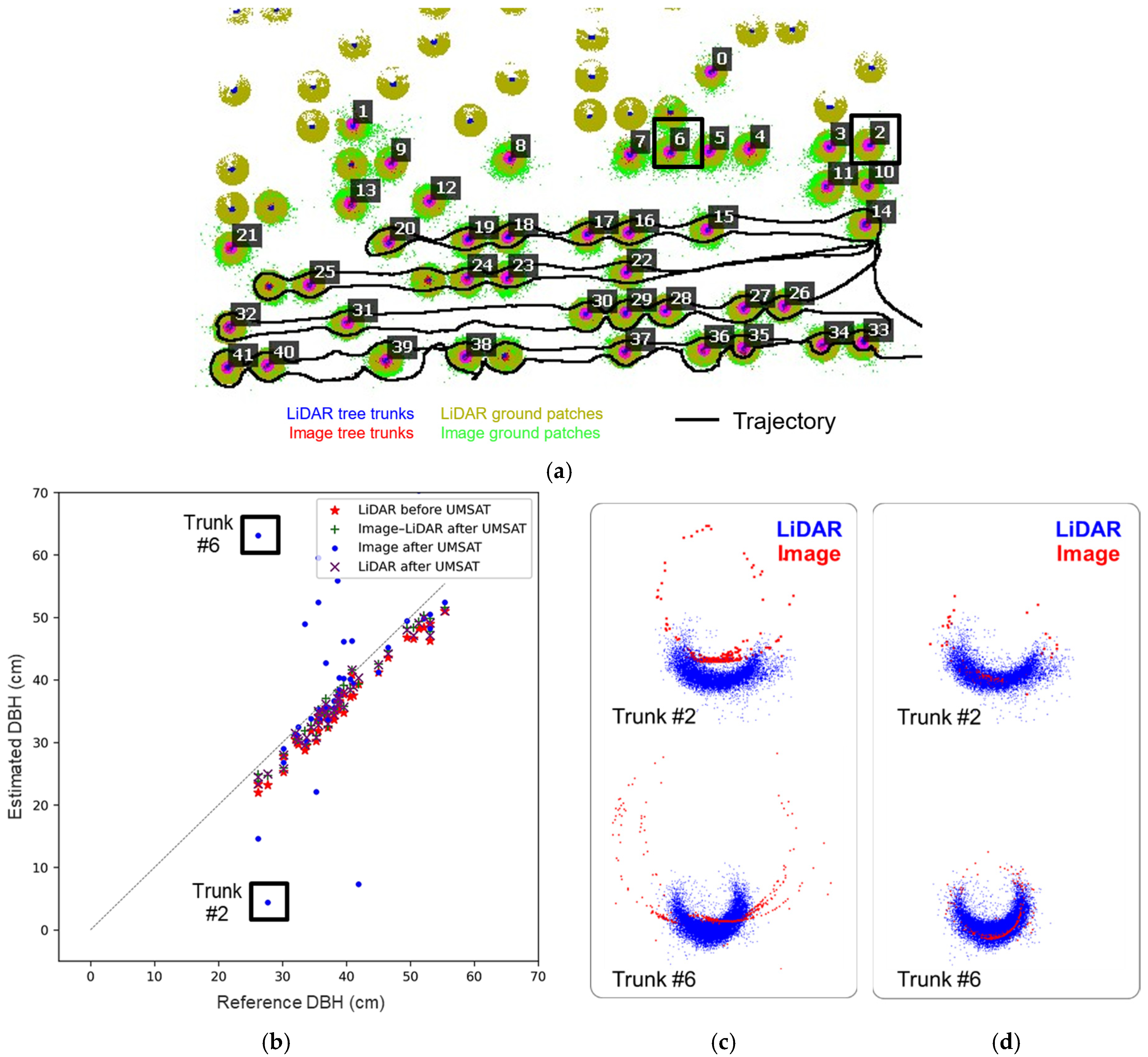
Figure 20a visualizes features in dataset A that have a reference value, where the features are labeled by trunk ID. Note that some trees were felled between the Backpack and reference data collections. Hence, their labels are missing in the figure. Figure 20b presents the estimated DBH in comparison to the reference values, and Table 9 reports the mean and RMS of their differences. The general trend among all scenarios is that the DBHs are consistently underestimated compared to the reference. A few possible reasons for this include reference data collected with calipers missing the fine bark details captured by sensors, and biases introduced in optimization due to partial scans or slight flattening of trunk arcs during initial reconstruction. That said, the image-based DBHs show several outliers around the line of equality. A closer inspection indicates that most of these outlier trunks are located far from the trajectory. As it turned out, the low density of image-based point clouds led to inaccurate initial estimates of cylindrical features, particularly for distant and incomplete trunks. In the absence of a reference, such as LiDAR data, the optimization only adjusts image-based points toward the initial model. Consequently, the feature-fitting function performs poorly in these cases during optimization, leading to inaccurate DBH estimates. Figure 20c,d illustrate the outcomes of the image-only and combined image-LiDAR optimizations, with each figure comparing image-based and LiDAR-derived features. In Figure 20c, there is a noticeable mismatch in both size and structure between the features, whereas in Figure 20d, the features are well aligned. These observations suggest that DBH estimates solely from image-based features far from the trajectory might not be reliable for tree inventory, and LiDAR-aiding is therefore necessary. Apart from the image-only estimates, all other outcomes, including those from the combined image–LiDAR optimization, produce DBH values consistent with those from LiDAR-only. Another observation from Table 9 is that the combined image–LiDAR optimization appears to improve the agreement of DBH with the reference—its mean difference is 1.1 cm lower than that of the initial LiDAR data from IS2-TEAM.
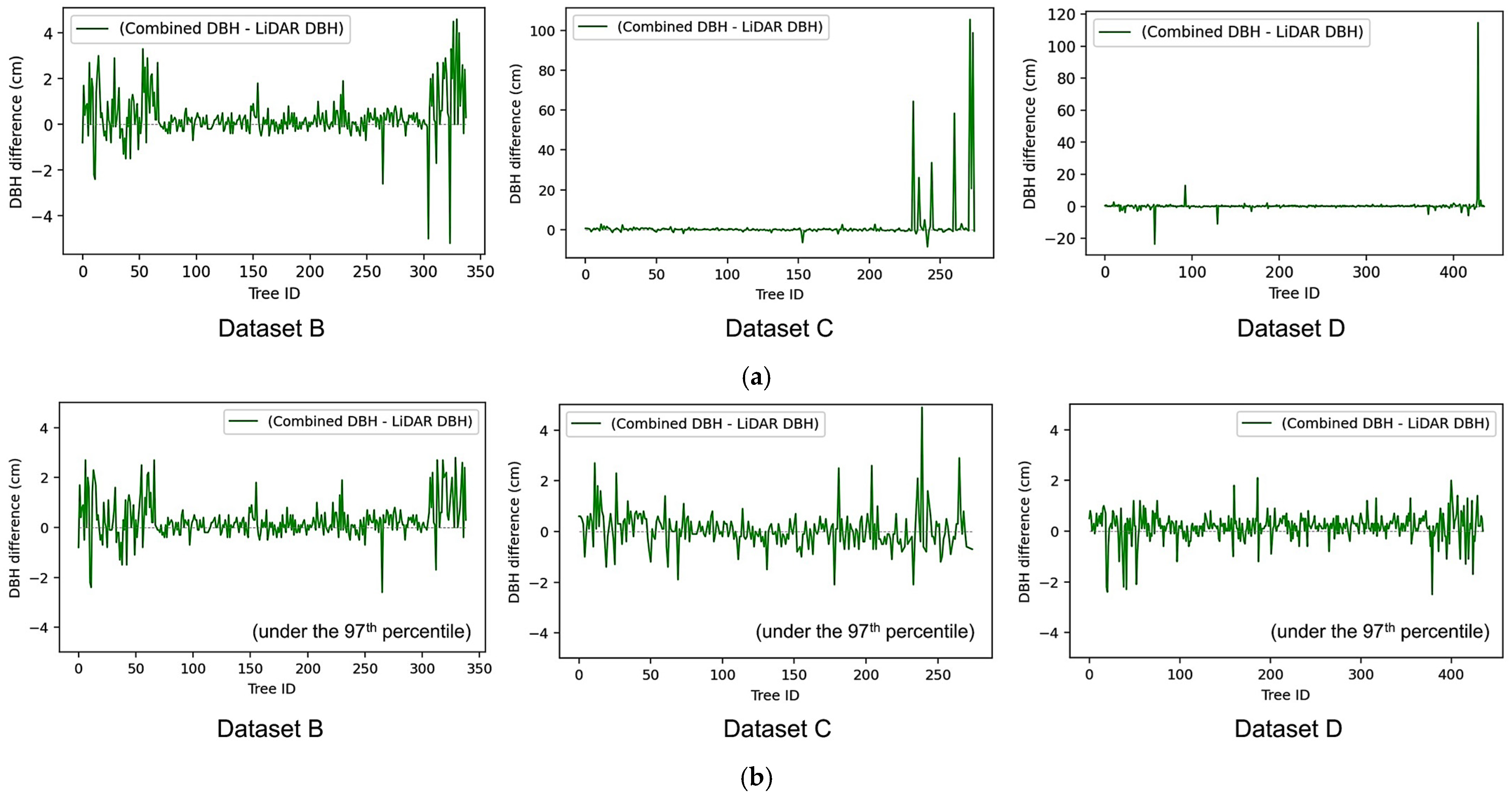
Since the image-only features may not be self-sufficient for DBH prediction, datasets B to D are assessed only between the LiDAR data from IS2-TEAM and the combined image and LiDAR data from UMSAT. Figure 21a shows the difference between the combined and LiDAR (IS2-TEAM)-based DBH values for each of the three datasets. While the differences are negligible in most areas of the plots, a few regions in each dataset show several prominent peaks. A close inspection of these irregularities reveals that the common sources of such large DBH estimates are sparse point clouds from images, and in rare cases, issues with the output of the tree segmentation pipeline, and false matches between image and LiDAR features. Figure 21b shows the same plots as Figure 21a, however, with values limited to under the 95th percentile. This second set of plots consistently shows differences within a few centimeters. Table 10 reports the mean and RMS differences between the two sets of DBH values (i.e., combined image–LiDAR from UMSAT and LiDAR-only from IS2-TEAM), computed for trunks having a difference of under 5 cm. These values corroborate the findings in Figure 21b, i.e., the mean differences are close to zero.

5. Discussion

All the various experiments with LiDAR and image-based point clouds demonstrate the effectiveness of the presented approach in aligning multi-modal 3D features. It is worth recalling that the proposed methodology includes target functions that also optimize feature model parameters. Thus, beyond improving multi-modal feature alignment, the methodology also refines the quality of individual features. Table 11 enumerates the numerical details related to feature quality for all four datasets before and after the sequential calibration and trajectory enhancement steps. One can notice that both the back-projection error and point-to-feature normal distances have reduced post optimization, indicating an improved feature definition. Furthermore, while the LiDAR-related metrics show an improvement of a few centimeters, the quality metrics for images, including back-projection error and point-to-feature normal distances, show over an order of magnitude improvement. This corroborates a larger adjustment of image features compared to those of LiDAR, as shown in the experiment section. Eventually, when it comes to the viability of imagery and LiDAR as separate modalities, experimental results prove that LiDAR offers more reliable structural information than imagery. Nonetheless, there is also an indication that integrating imagery with LiDAR may enhance point cloud alignment and DBH estimates, provided that the area of interest is carefully chosen.

6. Conclusions

This study addresses image–LiDAR misalignment by targeting Backpack hardware limitations and errors in system calibration and/or platform trajectory. In that regard, this paper’s contributions include the development of a Backpack MMS incorporating higher-frame-rate machine vision cameras, and an image–LiDAR data enhancement strategy to facilitate accurate tree inventory in a variety of forest environments. The images are used to generate SfM-based sparse points of the forest environment. Forest features, such as tree trunks and ground patches, provide geometric primitives useful for optimizing various calibration and trajectory-related parameters. Given the variation in positional accuracy across image and LiDAR trajectories, a global-structural criterion is defined to perform cross-modality feature matching. This strategy is shown to produce better matches than a simple spatial proximity-based approach.
Following the sequential system calibration and trajectory enhancement, the image–LiDAR feature alignment showed a notable improvement over the original features. The method eliminated misalignments of up to 1.1 m and 2 m along planimetric and vertical directions, respectively. For individual features, the point-to-feature RMS normal distance for image-based planes and cylinders improved as much as from 7.2 cm and 6.4 cm to 1.5 cm and 1.1 cm, respectively. Even in the case of LiDAR point clouds, which were already enhanced in IS2-TEAM, the combined feature-based trajectory enhancement refined the point-to-feature RMS normal distances from 1.9 cm and 2.9 cm to 1.1 cm and 0.85 cm, respectively. It is worth mentioning that, unlike most existing approaches, the optimization framework presented in this study offers the possibility to integrate LiDAR with imagery. For biometrics derivation, DBH values evaluated for a sample set of trees were found to be consistent between LiDAR-only and combined image–LiDAR estimates.
Although this study has proposed several contributions, many related topics could not be investigated in a single work. It is understood that even with elevated frame rates, imagery does not offer the same reliability in 3D reconstruction as LiDAR. Nonetheless, future research should examine how variations in camera frame rates affect optimization outcomes. In that regard, the workflow could be augmented to support multi-platform datasets, together with automation in feature extraction and an increase in computational efficiency for large datasets, ensuring the scalability of the approach. Additionally, future studies should incorporate enhanced path planning methods to reduce the occurrence of incomplete structures in LiDAR/image-based point clouds. The study sites may also encompass various forest types, including boreal and tropical forests, to determine whether variations in tree and ground structure affect the workflow. The analysis will involve examining the influence of understory on SfM-based reconstruction and evaluating the effectiveness of cross-modality feature matching in more complex forest scenarios, thereby providing additional validation of the method’s robustness.

Author Contributions

Conceptualization, R.M., S.F. and A.H.; methodology, R.M. and A.H.; data acquisition, R.M.; writing—original draft, R.M.; writing—review and editing, R.M., S.F. and A.H.; supervision, S.F. and A.H. All authors have read and agreed to the published version of the manuscript.

Funding

This research was funded by the U.S. Department of Agriculture’s National Institute of Food and Agriculture (NIFA), grant number 2023-68012-38992. The views and conclusions contained herein are those of the authors and should not be interpreted as representing the official policies, either expressed or implied, of the U.S. Government or NIFA.

Data Availability Statement

Processed data and derived products supporting the findings of this study are available from the corresponding author upon reasonable request.

Conflicts of Interest

The authors declare no conflicts of interest.

Appendix A

Georeferencing in a GNSS/INS-Based Backpack System

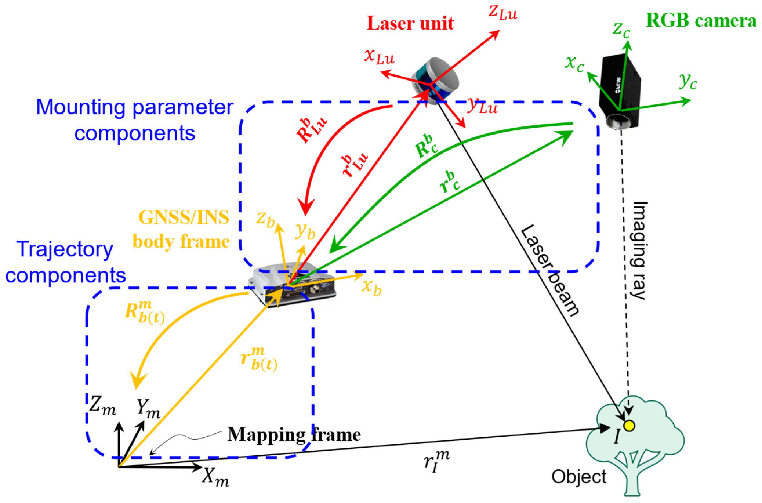
To understand the mechanism of georeferencing within a GNSS/INS-based Backpack system, Figure A1 illustrates the relationships between various sensors and the resulting 3D point coordinates from images and LiDAR. For a point I in 3D space captured by either the LiDAR or camera, its position in the mapping frame is determined by the spatial and rotational transformations that relate the sensor and mapping frames. This relationship is symbolically expressed by Equations (A1) and (A2), respectively, for the camera and LiDAR. Here, r b t m and R b t m are respectively the position and orientation parameters of the GNSS/INS body frame relative to the mapping frame. For a camera, r c b and R c b represent time-invariant mounting parameters (lever arm and boresight matrix, respectively). Given an image captured at time t , r i c t denotes the coordinates of the point i in the image coordinate frame, and the scale λ is the ratio between the distances of image and object space coordinates measured from the camera’s perspective center. In the case of LiDAR, r l u b and R l u b represent lever arm and boresight matrix, respectively, and r I l u ( t ) are coordinates of the LiDAR footprint captured at time t in the LiDAR unit coordinate frame.
Figure A1. Image/LiDAR point-positioning in mapping frame.
Remotesensing 18 01443 g0a1
r I m = r b t m + R b t m r c b + λ i , c , t R b t m R c b r i c t
r I m = r b t m + R b t m r l u b + R b t m R l u b r I l u ( t )

References

  1. West, P.W. Tree and Forest Measurement, 3rd ed.; Springer International Publishing: Cham, Switzerland, 2015; ISBN 978-3-319-14707-9. [Google Scholar]
  2. Bettinger, P.; Boston, K.; Siry, J.P.; Grebner, D.L. Forest Management and Planning, 2nd ed.; Academic Press: Cambridge, MA, USA, 2017; ISBN 9780128097069. [Google Scholar]
  3. Balestra, M.; Tonelli, E.; Vitali, A.; Urbinati, C.; Frontoni, E.; Pierdicca, R. Geomatic Data Fusion for 3D Tree Modeling: The Case Study of Monumental Chestnut Trees. Remote Sens. 2023, 15, 2197. [Google Scholar] [CrossRef]
  4. Zhang, Y.; Sun, H.; Zhang, F.; Zhang, B.; Tao, S.; Li, H.; Qi, K.; Zhang, S.; Ninomiya, S.; Mu, Y. Real-Time Localization and Colorful Three-Dimensional Mapping of Orchards Based on Multi-Sensor Fusion Using Extended Kalman Filter. Agronomy 2023, 13, 2158. [Google Scholar] [CrossRef]
  5. Trybała, P.; Morelli, L.; Remondino, F.; Farrand, L.; Couceiro, M.S. Under-Canopy Drone 3D Surveys for Wild Fruit Hotspot Mapping. Drones 2024, 8, 577. [Google Scholar] [CrossRef]
  6. Guan, T.; Shen, Y.; Wang, Y.; Zhang, P.; Wang, R.; Yan, F. Advancing Forest Plot Surveys: A Comparative Study of Visual vs. LiDAR SLAM Technologies. Forests 2024, 15, 2083. [Google Scholar] [CrossRef]
  7. Liu, H.; Xu, G.; Liu, B.; Li, Y.; Yang, S.; Tang, J.; Pan, K.; Xing, Y. A Real Time LiDAR-Visual-Inertial Object Level Semantic SLAM for Forest Environments. ISPRS J. Photogramm. Remote Sens. 2025, 219, 71–90. [Google Scholar] [CrossRef]
  8. Iglhaut, J.; Cabo, C.; Puliti, S.; Piermattei, L.; O’Connor, J.; Rosette, J. Structure from Motion Photogrammetry in Forestry: A Review. Curr. For. Rep. 2019, 5, 155–168. [Google Scholar] [CrossRef]
  9. Piermattei, L.; Karel, W.; Wang, D.; Wieser, M.; Mokroš, M.; Surový, P.; Koreň, M.; Tomaštík, J.; Pfeifer, N.; Hollaus, M. Terrestrial Structure from Motion Photogrammetry for Deriving Forest Inventory Data. Remote Sens. 2019, 11, 950. [Google Scholar] [CrossRef]
  10. Xu, Z.; Shen, X.; Cao, L. Extraction of Forest Structural Parameters by the Comparison of Structure from Motion (SfM) and Backpack Laser Scanning (BLS) Point Clouds. Remote Sens. 2023, 15, 2144. [Google Scholar] [CrossRef]
  11. White, J.C.; Coops, N.C.; Wulder, M.A.; Vastaranta, M.; Hilker, T.; Tompalski, P. Remote Sensing Technologies for Enhancing Forest Inventories: A Review. Can. J. Remote Sens. 2016, 42, 619–641. [Google Scholar] [CrossRef]
  12. Atkins, J.W.; Stovall, A.E.L.; Yang, X. Mapping Temperate Forest Phenology Using Tower, UAV, and Ground-Based Sensors. Drones 2020, 4, 56. [Google Scholar] [CrossRef]
  13. Di Stefano, F.; Chiappini, S.; Gorreja, A.; Balestra, M.; Pierdicca, R. Mobile 3D Scan LiDAR: A Literature Review. Geomat. Nat. Hazards Risk 2021, 12, 2387–2429. [Google Scholar] [CrossRef]
  14. Yang, S.; Xing, Y.; Xing, T.; Deng, H.; Xi, Z. Multisensors Fusion SLAM-Aided Forest Plot Mapping with Backpack Dual-LiDAR System. IEEE J. Sel. Top. Appl. Earth Obs. Remote Sens. 2024, 17, 16051–16070. [Google Scholar] [CrossRef]
  15. Goebel, M.; Iwaszczuk, D. Backpack System for Capturing 3D Point Clouds of Forests. ISPRS Ann. Photogramm. Remote Sens. Spat. Inf. Sci. 2023, X-1/W1-2023, 695–702. [Google Scholar] [CrossRef]
  16. Shin, Y.-H.; Shin, S.-Y.; Rastiveis, H.; Cheng, Y.-T.; Zhou, T.; Liu, J.; Zhao, C.; Varinlioğlu, G.; Rauh, N.K.; Matei, S.A.; et al. UAV-Based Remote Sensing for Detection and Visualization of Partially-Exposed Underground Structures in Complex Archaeological Sites. Remote Sens. 2023, 15, 1876. [Google Scholar] [CrossRef]
  17. Emesent. Hovermap LiDAR Scanner. Available online: https://emesent.com/emesent-product/hovermap-series/ (accessed on 18 August 2025).
  18. Leica Pegasus: Backpack Wearable Mobile Mapping Solution. Available online: https://leica-geosystems.com/en/products/mobile-mapping-systems/capture-platforms/leica-pegasus-backpack (accessed on 18 August 2025).
  19. Mosaic Xplor. Available online: https://www.mosaic51.com/products/mosaic-xplor/ (accessed on 18 August 2025).
  20. FARO. GeoSLAM ZEB Horizon RT Mobile Scanner. Available online: https://www.faro.com/en/Products/Hardware/GeoSLAM-ZEB-Horizon-RT (accessed on 31 August 2025).
  21. Parker, G.G.; Harding, D.J.; Berger, M.L. A Portable LiDAR System for Rapid Determination of Forest Canopy Structure. J. Appl. Ecol. 2004, 41, 755–767. [Google Scholar] [CrossRef]
  22. GreenValley International. LiBackpack DGC50H Backpack Laser Scanning. Available online: https://www.greenvalleyintl.com/LiBackpackDGC50H/ (accessed on 31 August 2025).
  23. Vandendaele, B.; Martin-Ducup, O.; Fournier, R.A.; Pelletier, G.; Lejeune, P. Mobile Laser Scanning for Estimating Tree Structural Attributes in a Temperate Hardwood Forest. Remote Sens. 2022, 14, 4522. [Google Scholar] [CrossRef]
  24. Hyyppä, E.; Yu, X.; Kaartinen, H.; Hakala, T.; Kukko, A.; Vastaranta, M.; Hyyppä, J. Comparison of Backpack, Handheld, under-Canopy UAV, and above-Canopy UAV Laser Scanning for Field Reference Data Collection in Boreal Forests. Remote Sens. 2020, 12, 3327. [Google Scholar] [CrossRef]
  25. Vatandaşlar, C.; Seki, M.; Zeybek, M. Assessing the Potential of Mobile Laser Scanning for Stand-Level Forest Inventories in near-Natural Forests. For. Int. J. For. Res. 2023, 96, 448–464. [Google Scholar] [CrossRef]
  26. Polewski, P.; Yao, W.; Cao, L.; Gao, S. Marker-Free Coregistration of UAV and Backpack LiDAR Point Clouds in Forested Areas. ISPRS J. Photogramm. Remote Sens. 2019, 147, 307–318. [Google Scholar] [CrossRef]
  27. LaRue, E.A.; Wagner, F.W.; Fei, S.; Atkins, J.W.; Fahey, R.T.; Gough, C.M.; Hardiman, B.S. Compatibility of Aerial and Terrestrial LiDAR for Quantifying Forest Structural Diversity. Remote Sens. 2020, 12, 1407. [Google Scholar] [CrossRef]
  28. Ouster LiDAR. Available online: https://ouster.com/insights/blog/the-camera-is-in-the-lidar (accessed on 18 August 2025).
  29. Zhao, C.; Hanafy, H.; Eissa, A.M.; Hany, Y.; Shao, J.; Fei, S.; Habib, A. Integration of Near-Proximal and Proximal Lidar Sensing for Fine-Resolution Forest Inventory. Photogramm. Eng. Remote Sens. 2026, 92, 189–211. [Google Scholar] [CrossRef]
  30. Cristóvão, M.P.; Portugal, D.; Carvalho, A.E.; Ferreira, J.F. A LiDAR-Camera-Inertial-GNSS Apparatus for 3D Multimodal Dataset Collection in Woodland Scenarios. Sensors 2023, 23, 6676. [Google Scholar] [CrossRef]
  31. Liang, Y.; Liu, J.; Lei, J.; Muhojoki, J.; Kukko, A.; Kaartinen, H.; Hyyppä, J.; Xu, D.; Zhang, W. Ground-to-Air Collaborative LiDAR Global Localization in Forest Environments. Expert Syst. Appl. 2026, 309, 131267. [Google Scholar] [CrossRef]
  32. He, F.; Habib, A. Automatic Orientation Estimation of Multiple Images with Respect to Laser Data. In Proceedings of the ASPRS 2014 Annual Conference, Louisville, KY, USA, 23–28 March 2014. [Google Scholar]
  33. Lv, F.; Ren, K. Automatic Registration of Airborne LiDAR Point Cloud Data and Optical Imagery Depth Map Based on Line and Points Features. Infrared Phys. Technol. 2015, 71, 457–463. [Google Scholar] [CrossRef]
  34. Wan, G.; Wang, Y.; Wang, T.; Zhu, N.; Zhang, R.; Zhong, R. Automatic Registration for Panoramic Images and Mobile LiDAR Data Based on Phase Hybrid Geometry Index Features. Remote Sens. 2022, 14, 4783. [Google Scholar] [CrossRef]
  35. Mastin, A.; Kepner, J.; Fisher, J. Automatic Registration of LiDAR and Optical Images of Urban Scenes. In Proceedings of the 2009 IEEE Conference on Computer Vision and Pattern Recognition; IEEE: Miami, FL, USA, 2009; pp. 2639–2646. [Google Scholar]
  36. Wang, R.; Ferrie, F.P. Automatic Registration Method for Mobile LiDAR Data. Opt. Eng. 2015, 54, 013108. [Google Scholar] [CrossRef]
  37. Hasheminasab, S.M.; Zhou, T.; Habib, A. Linear Feature-Based Image/LiDAR Integration for a Stockpile Monitoring and Reporting Technology. IEEE J. Sel. Top. Appl. Earth Obs. Remote Sens. 2023, 16, 2605–2623. [Google Scholar] [CrossRef]
  38. Hasheminasab, S.M.; Zhou, T.; Lin, Y.C.; Habib, A. Linear Feature-Based Triangulation for Large-Scale Orthophoto Generation over Mechanized Agricultural Fields. IEEE Trans. Geosci. Remote Sens. 2022, 60, 5621718. [Google Scholar] [CrossRef]
  39. Liu, L.; Stamos, I. A Systematic Approach for 2D-Image to 3D-Range Registration in Urban Environments. Comput. Vis. Image Underst. 2012, 116, 25–37. [Google Scholar] [CrossRef]
  40. Wang, Y.; Li, Y.; Chen, Y.; Peng, M.; Li, H.; Yang, B.; Chen, C.; Dong, Z. Automatic Registration of Point Cloud and Panoramic Images in Urban Scenes Based on Pole Matching. Int. J. Appl. Earth Obs. Geoinf. 2022, 115, 103083. [Google Scholar] [CrossRef]
  41. Habib, A.; Ghanma, M.; Morgan, M.; Al-Ruzouq, R. Photogrammetric and LiDAR Data Registration Using Linear Features. Photogramm. Eng. Remote Sens. 2005, 71, 699–707. [Google Scholar] [CrossRef]
  42. Berrio, J.S.; Shan, M.; Worrall, S.; Nebot, E. Camera-LiDAR Integration: Probabilistic Sensor Fusion for Semantic Mapping. IEEE Trans. Intell. Transp. Syst. 2022, 23, 7637–7652. [Google Scholar] [CrossRef]
  43. Yao, G.; Xuan, Y.; Chen, Y.; Pan, Y. Quantity-Aware Coarse-to-Fine Correspondence for Image-to-Point Cloud Registration. IEEE Sens. J. 2024, 24, 33826–33837. [Google Scholar] [CrossRef]
  44. Auat Cheein, F.; Steiner, G.; Perez Paina, G.; Carelli, R. Optimized EIF-SLAM Algorithm for Precision Agriculture Mapping Based on Stems Detection. Comput. Electron. Agric. 2011, 78, 195–207. [Google Scholar] [CrossRef]
  45. Shalal, N.; Low, T.; McCarthy, C.; Hancock, N. Orchard Mapping and Mobile Robot Localisation Using On-Board Camera and Laser Scanner Data Fusion—Part A: Tree Detection. Comput. Electron. Agric. 2015, 119, 254–266. [Google Scholar] [CrossRef]
  46. Huang, R.; Zheng, S.; Hu, K. Registration of Aerial Optical Images with LiDAR Data Using the Closest Point Principle and Collinearity Equations. Sensors 2018, 18, 1770. [Google Scholar] [CrossRef]
  47. Zhou, T.; Hasheminasab, S.M.; Habib, A. Tightly-Coupled Camera/LiDAR Integration for Point Cloud Generation from GNSS/INS-Assisted UAV Mapping Systems. ISPRS J. Photogramm. Remote Sens. 2021, 180, 336–356. [Google Scholar] [CrossRef]
  48. Zhou, T.; Hasheminasab, S.M.; Ravi, R.; Habib, A. LiDAR-Aided Interior Orientation Parameters Refinement Strategy for Consumer-Grade Cameras Onboard UAV Remote Sensing Systems. Remote Sens. 2020, 12, 2268. [Google Scholar] [CrossRef]
  49. Li, J.; Yang, B.; Chen, C.; Huang, R.; Dong, Z.; Xiao, W. Automatic Registration of Panoramic Image Sequence and Mobile Laser Scanning Data Using Semantic Features. ISPRS J. Photogramm. Remote Sens. 2018, 136, 41–57. [Google Scholar] [CrossRef]
  50. Eslami, M.; Saadatseresht, M. Imagery Network Fine Registration by Reference Point Cloud Data Based on the Tie Points and Planes. Sensors 2021, 21, 317. [Google Scholar] [CrossRef]
  51. Wen, N.; Wang, X.; Guo, J.; Wang, Y.; Wang, Y. Multi-Modal Fusion of LiDAR and Camera Sensors for Enhanced Perception in Intelligent Traffic Systems. In Proceedings of the 2024 International Conference on Electronic Engineering and Information Systems (EEISS); IEEE: Changsha, China, 2024; pp. 166–174. [Google Scholar]
  52. Yang, B.; Chen, C. Automatic Registration of UAV-Borne Sequent Images and LiDAR Data. ISPRS J. Photogramm. Remote Sens. 2015, 101, 262–274. [Google Scholar] [CrossRef]
  53. NovAtel. PwrPak7-E1 Datasheet 2025; NovAtel Inc.: Calgary, AB, Canada, 2025. [Google Scholar]
  54. Velodyne VLP16 Puck. Available online: https://ouster.com/products/hardware/vlp-16 (accessed on 19 August 2025).
  55. Teledyne Vision Solutions. Grasshopper3 GigE. Available online: https://www.teledynevisionsolutions.com/products/grasshopper3-gige/?model=GS3-PGE-91S6C-C&vertical=machine%20vision&segment=iis (accessed on 19 August 2025).
  56. Habib, A.; Morgan, M. Stability Analysis and Geometric Calibration of Off-the-Shelf Digital Cameras. Photogramm. Eng. Remote Sens. 2005, 71, 733–741. [Google Scholar] [CrossRef]
  57. Ravi, R.; Lin, Y.-J.; Elbahnasawy, M.; Shamseldin, T.; Habib, A. Simultaneous System Calibration of a Multi-LiDAR Multicamera Mobile Mapping Platform. IEEE J. Sel. Top. Appl. Earth Obs. Remote Sens. 2018, 11, 1694–1714. [Google Scholar] [CrossRef]
  58. Habib, A.; Lay, J.; Wong, C. Specifications for the Quality Assurance and Quality Control of LiDAR Systems. Base Mapping and Geomatic Services of British Columbia 2006. Available online: https://engineering.purdue.edu/CE/Academics/Groups/Geomatics/DPRG/files/LIDARErrorPropagation.zip (accessed on 19 August 2025).
  59. Zhao, C.; Zhou, T.; Fei, S.; Habib, A. Forest Feature LiDAR SLAM (F2-LSLAM) and Integrated Scan Simultaneous Trajectory Enhancement and Mapping (IS2-TEAM) for Accurate Forest Inventory Using Backpack Systems. Int. Arch. Photogramm. Remote Sens. Spat. Inf. Sci. 2023, XLVIII-1/W2-2023, 1823–1830. [Google Scholar] [CrossRef]
  60. Agisoft Metashape Professional, Version 2.2.0; Agisoft LLC: St. Petersburg, Russia, 2024. Available online: https://www.agisoft.com/downloads/installer/ (accessed on 19 August 2025).
  61. Friedman, J.H.; Bentley, J.L.; Finkel, R.A. An Algorithm for Finding Best Matches in Logarithmic Expected Time. ACM Trans. Math. Softw. 1977, 3, 209–226. [Google Scholar] [CrossRef]
  62. Zhou, T.; Ravi, R.; Lin, Y.-C.; Manish, R.; Fei, S.; Habib, A. In Situ Calibration and Trajectory Enhancement of UAV and Backpack LiDAR Systems for Fine-Resolution Forest Inventory. Remote Sens. 2023, 15, 2799. [Google Scholar] [CrossRef]
  63. Zhao, C.; Fei, S.; Habib, A. Integrated Scan Simultaneous Trajectory Enhancement and Mapping (IS2-TEAM) for Fine Resolution Forest Inventory Using Backpack LiDAR. Remote Sens. Environ. 2026, 334, 115212. [Google Scholar] [CrossRef]
  64. Chen, S.; Liu, H.; Feng, Z.; Shen, C.; Chen, P. Applicability of Personal Laser Scanning in Forestry Inventory. PLoS ONE 2019, 14, e0211392. [Google Scholar] [CrossRef]
  65. Crouse, D.F. On Implementing 2D Rectangular Assignment Algorithms. IEEE Trans. Aerosp. Electron. Syst. 2016, 52, 1679–1696. [Google Scholar] [CrossRef]
  66. Zhou, T.; Liu, J.; Shin, S.; Habib, A. Multi-Primitive Triangulation of Airborne and Terrestrial Mobile Mapping Image and LiDAR Data. Int. Arch. Photogramm. Remote Sens. Spat. Inf. Sci. 2023, XLVIII-1/W1-2023, 587–594. [Google Scholar] [CrossRef]
Figure 1. Visualization of 2D rendering and 3D reconstruction from LiDAR point cloud and RGB images: (a) 2D rendering and (b) LiDAR point cloud overlaid with LiDAR and image-based 3D features (left and right columns are respectively based on accurate and inaccurate system calibration/trajectory parameters).
Remotesensing 18 01443 g001
Figure 2. Planned layout of the system, and FOV of its LiDAR sensor and cameras (yellow and green colors refer to LiDAR and camera FOV, respectively).
Remotesensing 18 01443 g002
Figure 3. The complete Backpack MMS with its various components.
Remotesensing 18 01443 g003
Figure 4. Data and power distribution schemes for the proposed Backpack LiDAR–camera system: (a) data distribution scheme and (b) power supply scheme.
Remotesensing 18 01443 g004
Figure 5. Workflow of the proposed Backpack LiDAR–camera system calibration/trajectory enhancement.
Remotesensing 18 01443 g005
Figure 6. Sample LiDAR and image-based point clouds from the same mission.
Remotesensing 18 01443 g006
Figure 7. Pipeline for segmenting individual trees and deriving forest biometrics [29]: (a) flowchart of the forestry pipeline, (b) sample AG point cloud colored by height, (c) segmented point cloud randomly colored by tree ID, and (d) extracted tree trunks randomly colored by trunk ID.
Remotesensing 18 01443 g007
Figure 8. Visualization of tree trunks and ground patches extracted from LiDAR point clouds.
Remotesensing 18 01443 g008
Figure 9. Illustration of the simple spatial proximity-based approach for feature matching: (a) correct matches as reference and (b) one of several possible sets of matches based on spatial proximity.
Remotesensing 18 01443 g009
Figure 10. Illustration of stages of the proposed global–structural approach for matching image–LiDAR features: (a) all possible conjugate pairs, (b) potential matches after applying distance filter, (c) identification of nearest-neighbors, (d) example of distance normalization, and (e) final matches after optimization. Solid arrows indicate matched pairs; dashed arrows indicate neighboring pairs.
Remotesensing 18 01443 g010
Figure 11. Comparison of feature matching results obtained using the spatial proximity-based approach and the proposed method for a given camera–LiDAR pair of a sample forest dataset: (a) result from the spatial proximity-based approach (colored randomly by match ID), (b) result from the proposed global–structural approach (colored randomly by match ID), (c) lines connecting corresponding image–LiDAR features (colored by displacement magnitude), and (d) histogram of the displacements between corresponding features.
Remotesensing 18 01443 g011aRemotesensing 18 01443 g011b
Figure 12. Pictorial representation of the minimization residual for various features used in this study: (a) point-to-plane normal distance, (b) point-to-cylinder normal distance, and (c) back-projection error. Residual distances are highlighted in red; dashed arrows in (c) indicate imaging ray. PC: perspective center; ND: normal distance.
Remotesensing 18 01443 g012
Figure 13. Visualization of a trajectory point and its neighboring reference points.
Remotesensing 18 01443 g013
Figure 14. Details of the study sites: (a) location on map (source: Google Maps) and (b) leaf condition during data acquisition.
Remotesensing 18 01443 g014
Figure 15. Visualization of the extracted image–LiDAR features from various datasets: (a) dataset A, (b) dataset B, (c) dataset C, and (d) dataset D (trajectories are colored by time and all point clouds are shown in top view).
Remotesensing 18 01443 g015
Figure 16. Illustration of various coordinate systems and fixed rotations applied to the camera coordinate system to avoid gimbal lock: (a) sensors and their coordinate systems, (b) rotations applied to the left camera coordinate system, and (c) rotations applied to the right camera coordinate system.
Remotesensing 18 01443 g016
Figure 17. Visualization of image–LiDAR feature alignment before and after system calibration for dataset A: (a) overview of the image–LiDAR features after camera system calibration; and (b,c) alignment of sample features (as highlighted in (a)) before and after calibration along with reported DBH (estimated and reference). Trajectory is colored by time.
Remotesensing 18 01443 g017
Figure 18. Visualization of feature alignment before and after trajectory/point cloud enhancement for various experiments: (a) experiment 2 (dataset A), (b) experiment 3 (dataset B), (c) experiment 4 (dataset C), and (d) experiment 5 (dataset D).
Remotesensing 18 01443 g018aRemotesensing 18 01443 g018b
Figure 19. Rendering of sample LiDAR-to-image back-projections for various datasets before and after system calibration and trajectory enhancement: (a) dataset A, (b) dataset B, (c) dataset C, and (d) dataset D. The boxes in the overview figures on the left indicate the locations of the trunks used in the corresponding illustrations.
Remotesensing 18 01443 g019aRemotesensing 18 01443 g019b
Figure 20. Visualization of trunks in dataset A and comparison of DBH estimates with the reference data: (a) overview of the available reference features labeled by trunk ID, (b) plot of the DBH estimates against the reference for various optimization scenarios, (c) sample trunks (as highlighted with boxes in (a,b)) after image-only optimization compared with LiDAR-derived features, and (d) same trunks as in (c) but with results after a combined image-LiDAR optimization.
Remotesensing 18 01443 g020
Figure 21. Comparison of DBH estimates for various datasets with and without outliers: (a) differences in the DBH from IS2-TEAM and those from combined image–LiDAR optimization (UMSAT), and (b) DBH differences limited to those under 97th percentile.
Remotesensing 18 01443 g021
Table 1. Specifications of various sensors on the proposed Backpack MMS.
GNSS/INS Unit *
ModelPositional Accuracy (cm)Attitude Accuracy (deg)
HorizontalVerticalRoll/PitchHeading
NovAtel PwrPak7-E1
(IMU rate: 125 Hz)
1 cm2 cm0.008°0.038°
LiDARCamera
ModelVelodyne VLP-16ModelFLIR Grasshopper 3
Number of laser beams16Camera typeFrame w/global shutter
Number of returns2Sensor type/format1″ Sony CCD
Horizontal FOV360 ° Focal length8 mm
Vertical FOV−15 ° to +15 ° FOV(H × V): 83.5 ° × 68 °
Range100 mImage dimensions3376 × 2704 pixels (9.1 MP)
Ranging accuracy ± 3 cmAcquisition rate 3 frames/s (configured)
Pulse rate (single return)300,000 pts./sPixel size3.69 μ m
Wavelength905 nmSpectral bands3 bands (RGB)
* Manufacturer-specified post-processed performance.
Table 2. Description of the experimental datasets.
IDStudy Site
(and Tree Species)
DateForest TypeDurationNum. of LiDAR pts.
(in Millions)
Num. of Images
(Cam 1 and 2)
APlot 1B
(Black Walnut)
24 July 2024
(Leaf-on)
Well-managed plantation~12 min144 2021 and 2021
BPlot 115
(2007 Red and Burr Oak)
6 April 2025
(Leaf-off)
Young plantation~13 min1702284 and 2250
CPlot 4D
(Multiple species)
6 April 2025
(Leaf-off)
Natural~15 min2092620 and 2572
DPlot 3B
(1962 Red Oak)
8 April 2025
(Leaf-off)
Mature plantation
(w/complex structure)
~26 min3314659 and 4655
Table 3. Summary of the extracted image and LiDAR features.
Imagery (FLIR Grasshopper3)
PropertiesDataset ADataset BDataset CDataset D
Cam 1 (Left)Cam 2 (Right)Cam 1 (Left)Cam 2 (Right)Cam 1 (Left)Cam 2 (Right)Cam 1 (Left)Cam 2 (Right)
Number of photos involved16071773176419542611251942033917
Number of features
(Tree trunks/ground patches)
48/4841/41205/190200/200209/209233/231331/331416/412
Total number of image measurements900,4481,712,1361,719,7942,313,9054,269,4533,906,7164,203,6935,031,212
Total number of tie points314,101559,712748,240977,1541,767,3871,587,8091,636,0701,832,486
Ratio of image measurements to tie points2.93.12.32.42.42.52.62.7
LiDAR (Velodyne VLP-16)
PropertiesDataset ADataset BDataset CDataset D
Number of features
(Tree trunks/ground patches)
159/159643/643587/587556/556
Total number of LiDAR points
(Tree trunks/ground patches)
5,955,659/4,265,5905,336,933/8,661,21312,030,397/14,713,90716,110,081/14,421,305
Table 4. Initial and adjusted camera mounting parameters based on the proposed strategy.
Camera 1 (Left) Mounting Parameters
Δ X m Δ Y m Δ Z m Δ ω ° Δ ϕ ° Δ κ °
Initial0.000−0.1500.100−0.0120.1440.696
Adjusted−0.110−0.0650.1010.128−0.0120.098
Camera 2 (Right) Mounting Parameters
Δ X m Δ Y m Δ Z m Δ ω ° Δ ϕ ° Δ κ °
Initial0.0100.017−0.008−0.313−0.004−0.008
Adjusted0.101−0.062−0.040−0.155−0.161−0.106
Table 5. Estimated planimetric and vertical discrepancies between image–LiDAR features of dataset A before and after calibration.
TypeMean Discrepancy (Image Minus LiDAR)
Before CalibrationAfter Calibration
Planimetric d x :   0.33 ± 0.17   m<0.05 m
d y :   1.01 ± 0.27   m<0.05 m
Vertical d z : 0.32 ± 0.23   m<0.05 m
Table 6. Quality metrics for image and LiDAR features from experiments 1–2 (dataset A), i.e., before calibration, after calibration, and after sequential calibration and trajectory enhancement (all values are RMS).
MetricsBefore CalibrationAfter CalibrationAfter Calibration and Trajectory Enhancement
Back-projection error44.6 px1.7 px0.9 px
Image object point-to-plane normal dist.3.5 cm0.9 cm0.85 cm
Image object point-to-cylinder normal dist.6.1 cm0.9 cm0.66 cm
LiDAR point-to-plane normal dist.1.5 cm1.1 cm1.05 cm
LiDAR point-to-cylinder normal dist.2.9 cm0.9 cm0.85 cm
Table 7. Estimated planimetric and vertical discrepancies between image and LiDAR features before calibration and after sequential calibration and trajectory enhancement.
DatasetTypeMean Discrepancy (Image Minus LiDAR)
Before CalibrationAfter Calibration and Trajectory Enhancement
BPlanimetric d x :   0.33 ± 0.21   m
d y :   0.38 ± 0.19   m
<0.05 m
Vertical d z :   0.66 ± 0.37   m <0.05 m
CPlanimetric d x :   0.15 ± 0.25   m
d y :   0.13 ± 0.29   m
<0.05 m
Vertical d z :   2.10 ±   0.93   m <0.05 m
DPlanimetric d x :   0.81 ± 0.44   m
d y :   0.59 ± 0.52   m
<0.05 m
Vertical d z : 1.15 ± 0.72   m <0.05 m
Table 8. Adjustments applied to pose parameters after trajectory enhancement (all values are RMS).
Experiment ID X (cm) Y (cm) Z (cm) ω (deg) ϕ (deg) κ (deg)
2 (dataset A)0.850.731.180.0160.0130.025
3 (dataset B)0.600.530.840.0140.0220.020
4 (dataset C)0.780.791.130.0270.0270.023
5 (dataset D)1.041.390.800.0220.0450.028
Table 9. Comparison of DBH estimates against the reference for various optimization scenarios of dataset A (unless otherwise noted, all values are computed for 42 reference DBH).
ScenarioMean Diff. (cm)RMS Diff. (cm)Remarks
LiDAR-only (before UMSAT)−3.23.4Based on IS2-TEAM trajectory
Combined image–LiDAR (UMSAT)−2.12.5
Image-only (UMSAT)−1.82.2Computed for 26 trunks with abs. diff <5 cm
LiDAR-only (UMSAT)−2.42.7
Table 10. DBH comparison between LiDAR (IS2-TEAM) and the combined image–LiDAR (UMSAT) estimates for various datasets.
Image–LiDAR DBH Minus LiDAR (IS2-TEAM) DBH
Number of Trunks Used for
DBH Calculation
Mean Diff. (cm)RMS Diff. (cm)
Dataset B231 out of 3380.120.42
Dataset C268 out of 2750.000.98
Dataset D432 out of 4360.130.82
Table 11. Quality metrics for image and LiDAR features from experiments 2–5 before and after all enhancements (all values are RMS).
MetricsExp. 2
(Dataset A)
Exp. 3
(Dataset B)
Exp. 4
(Dataset C)
Exp. 5
(Dataset D)
Before/AfterBefore/AfterBefore/AfterBefore/After
Back-projection error44.6 px/0.9 px21.0 px/1.0 px33.2 px/1.8 px95.7 px/1.4 px
Image object point-to-plane normal dist.3.5 cm/0.9 cm5.3 cm/1.2 cm10 cm/0.9 cm7.2 cm/1.5 cm
Image object point-to-cylinder normal dist.6.1 cm/0.7 cm4.6 cm/0.9 cm3.6 cm/2.6 cm6.4 cm/1.1 cm
LiDAR point-to-plane normal dist.1.5 cm/1.1 cm1.8 cm/1.2 cm1.9 cm/1.1 cm1.5 cm/1.1 cm
LiDAR point-to-cylinder normal dist.2.9 cm/0.9 cm1.8 cm/1.0 cm2.3 cm/1.0 cm2.8 cm/1.1 cm
Disclaimer/Publisher’s Note: The statements, opinions and data contained in all publications are solely those of the individual author(s) and contributor(s) and not of MDPI and/or the editor(s). MDPI and/or the editor(s) disclaim responsibility for any injury to people or property resulting from any ideas, methods, instructions or products referred to in the content.