Article

Daily-Scale Meteorological Normalization of Surface Solar Radiation in Varying Pollution Levels: A Statistical Case Study in Beijing (2015–2019)


1
The School of Aviation Meteorology, Civil Aviation Flight University of China, No. 46, Section 4, Nanchang Road, Guanghan 618307, China
2
The School of Geo-Science and Technology, Zhengzhou University, No. 75, Daxue North Road, Zhengzhou 450001, China
*
Author to whom correspondence should be addressed.
Remote Sens. 2026, 18(9), 1368; https://doi.org/10.3390/rs18091368
Submission received: 1 March 2026 / Revised: 11 April 2026 / Accepted: 21 April 2026 / Published: 29 April 2026
(This article belongs to the Special Issue Advanced AI Technology for Remote Sensing Analysis (Second Edition))

Highlights

What are the main findings?
  • Meteorological controls on daily surface solar radiation in Beijing vary systematically with pollution level, with cloud cover and RH showing strong associations and diffuse radiation exhibiting the clearest pollution-dependent shift.
  • RF reproduced daily radiation components with strong predictive performance (R2 = 0.83–0.88), and RF- and MLR-derived adjusted anomalies showed broadly consistent temporal variations (r = 0.63–0.78).
What are the implications of the main findings?
  • Daily radiation–pollution relationships are strongly confounded by meteorological variability, so meteorological influences should be explicitly accounted for in daily radiation analyses.
  • RF-based meteorological normalization is a practical tool for daily station radiation records and may be extended to multi-site analyses and finer temporal resolution.

Abstract

Surface solar radiation at the ground is affected by aerosols, clouds, and atmospheric moisture, as well as by circulation-related conditions that influence cloud formation and pollutant transport. In daily observations, these influences are mixed, which makes pollution-related variability difficult to interpret. We analyzed data from Beijing station 54511 (2015–2019), including daily integrated radiation components and collocated meteorological and pollution variables. We used wavelet coherence, pollution-stratified association analysis, and gray relational analysis, and compared two meteorological normalization methods: multiple linear regression (MLR) and random forest (RF). The results show that meteorological–radiation relationships vary systematically across pollution levels, indicating substantial meteorological confounding in daily radiation analyses. Among the radiation components, DR shows the clearest pollution-dependent shift in its relationship with RH, while several direct components become less sensitive to cloud cover under heavier pollution. RF reproduced daily radiation components with strong predictive performance (R2 = 0.83–0.88), and the meteorologically adjusted anomalies from RF were consistent with those from MLR (r = 0.63–0.78 across components). These findings suggest that both MLR and RF can be effectively used to normalize meteorological effects in daily station records. The analysis supports routine interpretation of day-to-day surface radiation variability and can be extended to multi-site studies and finer temporal resolution.

1. Introduction

As the primary energy source for the Earth, solar radiation drives key physical processes, such as atmospheric and ocean circulation and sea–land breeze circulation in coastal regions [1,2,3,4], and plays a significant role in biogeochemical cycles [5,6]. As climate change increasingly alters atmospheric patterns and environmental systems, understanding the variability of surface solar radiation becomes important not only for Earth-system science but also for the efficient development and use of solar energy, which can help reduce environmental pollution and dependence on fossil fuels [7,8,9,10,11]. However, the amount and composition of solar radiation reaching the surface are influenced by many factors, such as aerosols, clouds, and land surface. Surface radiation components vary with location, season, and time [12]. Meteorological conditions significantly influence surface radiation, such as through the absorption and reflection effects of clouds and water vapor [13,14]. Recent studies have further emphasized that clouds and aerosols are key drivers of spatiotemporal variability in surface solar irradiance, especially in conjunction with water vapor variability [15,16]. At the same time, increasing anthropogenic particulate emissions can reduce surface solar radiation through aerosol scattering and absorption [17,18,19], and can also alter diffuse radiation under haze and dust conditions [20]. Understanding the influence of anthropogenic emissions on radiation components is therefore important for improving our understanding of the surface energy balance and for supporting the efficient use of solar energy. However, this relationship is not strictly unidirectional, because radiation can also influence pollution through photochemical and boundary-layer processes. Yet meteorological conditions change rapidly and influence surface radiation in complex ways, introducing substantial uncertainty into analyses of aerosol-related radiation changes. Therefore, meteorological influences need to be explicitly accounted for when examining radiation–pollution relationships. In this context, it is also necessary to evaluate whether meteorological normalization methods, including RF-based approaches, can effectively reduce this source of uncertainty.
The influence of meteorological conditions on solar radiation components is complex, and meteorology also affects the dispersion and accumulation of anthropogenic pollutants. Previous studies have shown that cloud type and cloud amount directly affect surface solar radiation, and recent studies have further highlighted the important role of cloud cover in modulating surface solar irradiance [21,22,23]. Because cloud macrophysical and microphysical properties vary strongly, clouds remain a major source of uncertainty in climate simulation and prediction [24,25]. Clouds affect the solar radiation reaching the surface through reflection and absorption [21,23], and they can further modify surface scattering through interactions with aerosols [26,27]. Water vapor has a similarly strong influence because it directly absorbs solar radiation [28,29] and can also alter aerosol-related radiative effects by changing aerosol hygroscopic growth and optical properties [30,31,32]. In addition, meteorological conditions influence particulate matter concentrations, which in turn affect the surface energy budget. Adverse weather conditions and pollutant accumulation can reinforce each other within the boundary layer, leading to stronger radiation attenuation [33,34]. Together, these processes increase uncertainty in the evaluation of aerosol-related radiation changes and can also complicate assessments of pollution control effectiveness [25,35,36]. Despite this, there is still limited discussion of how the statistical relationships between meteorological factors and surface solar radiation vary under different pollution conditions. A clearer description of these relationships is needed to better understand the importance of separating meteorological influences from anthropogenic emission effects in daily radiation analyses. This study will describe the relationship between meteorological conditions and surface solar radiation under different pollution conditions through statistical analysis to demonstrate the necessity of meteorological normalization.
At present, chemical transport models and other physically based atmospheric modeling frameworks are widely used to investigate the influence of anthropogenic pollutant emissions on surface solar radiation. However, model-based estimates are often affected by uncertainties in emission inventories, parameter settings, and process representation. To reduce these uncertainties, statistical methods have increasingly been used to adjust for meteorological influences, especially in air quality studies. These methods include Bayesian hierarchical models [37], generalized additive models [38], nonparametric regression [39], and multiple linear regression (MLR) [40]. More recently, machine-learning methods, especially tree-based models such as RF, have been used for meteorological normalization because they can capture nonlinear relationships and interactions among predictors more effectively [41]. Although RF-based meteorological normalization has been widely applied in air quality attribution studies, its use in daily surface radiation analysis requires careful interpretation. At daily temporal resolution, the main goal is statistical adjustment and a robust assessment of radiation–pollution relationships, rather than a direct diagnosis of aerosol–radiation or aerosol–cloud interaction mechanisms.
Accordingly, this study has two main objectives. First, it quantifies how meteorological–radiation relationships at the daily scale change across pollution levels, with particular attention paid to the differential responses of individual radiation components. Second, it evaluates whether RF-based meteorological normalization provides results consistent with those of a conventional MLR-based adjustment, thereby assessing the robustness and practical utility of RF for daily radiation analysis. Beyond the use of multiple statistical tools, the study aims to identify pollution-dependent shifts in the apparent meteorological controls on radiation and to provide quantitative evidence on the consistency of the two normalization frameworks. The data and methods are described in Section 2, the results are presented in Section 3, the discussion is presented in Section 4, and the conclusions are presented in Section 5.

2. Data and Methods

2.1. Data

In this study, meteorological data and surface solar radiation observations from Beijing station (No. 54511) were collected for the core analysis period of 2015–2019. The supplementary time-series figures are intended only to show the temporal evolution of the daily record and are not used for annual trend estimation. The analyses presented in this study focus on daily-scale relationships, time–frequency coherence, and meteorologically normalized as well as deseasonalized/detrended comparisons. The daily surface solar radiation (MJm−2day−1) observations used in this study were obtained from National Meteorological Information Center (NMIC, http://data.cma.cn/), including total solar radiation (TR), net radiation (NR), diffuse radiation (DR), horizontal direct solar radiation (HDR), reflected radiation (RR) and vertical direct solar radiation (VDR, i.e., direct-beam solar radiation incident on a plane perpendicular to the solar beam). These radiation data come from the national radiation observation system of the China Meteorological Administration. Previous studies describing the same observation system indicate that global, direct, and diffuse radiation are measured using pyranometers, pyrheliometers, and shaded pyrheliometers, respectively, with regular calibration and quality-control procedures applied [42]. In this study, only quality-controlled daily integrated radiation records were used. We obtained daily values for several meteorological variables: air pressure (P, hPa), air temperature (T, °C), precipitation (PRE, mm), relative humidity (RH, %), wind direction (WD, °), wind speed (WS, m/s), surface temperature (ST, °C), and visibility (VIS, km). The daily value of the total cloud cover (TCC), low cloud cover (LCC) and the boundary layer height (BLH, m), and vertical integral of mass of atmosphere (VMA, kg m−2, i.e., the total mass of air in the atmospheric column per unit area) data are all obtained from the fifth generation European Centre for Medium-Range Weather Forecasts (ECMWF) reanalysis (ERA5) hourly data on single levels from 1979 to present (0.25° × 0.25°, https://cds.climate.copernicus.eu/). Aerosol optical depth (AOD) data were obtained from the Modern-Era Retrospective Analysis for Research and Applications, Version 2 (MERRA-2, 0.5° × 0.65°, https://disc.gsfc.nasa.gov/). In addition, the PM2.5 values used in this study were obtained from the Beijing Municipal Environmental Monitoring Center (http://www.bjmemc.com.cn). ERA5 and MERRA-2, as reanalysis-based products, may still be affected by uncertainties related to model representation and spatial representativeness.
Based on the variables described above, we divided them into four categories: meteorological variables (P, VMA, T, ST, RH, WD, WS, PRE, LCC, TCC, BLH), pollution-related variables (VIS, AOD, PM2.5), time variables (time_x and time_y: cyclic encoding of the day of year using sine and cosine transforms, respectively; Unix: the total number of seconds since 00:00:00 on 1 January 1970) and prediction variables (TR, NR, DR, HDR, RR, VDR). When training the RF model, variables other than prediction variables are used as input variables of the model.

2.2. Methods

To assess the influence of meteorological factors on surface solar radiation and to evaluate the effectiveness of meteorological adjustments at a daily scale, we employed wavelet transform coherence, statistical analysis, and gray relational analysis. We examined how relationships between meteorological factors and radiation components vary across pollution levels. Pollution levels were classified using PM2.5 mass concentration thresholds: clean air (PM2.5 < 75 μg/m3), moderate pollution (75–150 μg/m3), and severe pollution (PM2.5 > 150 μg/m3) [43]. We further compared meteorologically adjusted radiation anomalies derived from multiple linear regression (MLR) and a random-forest (RF) approach to assess the consistency of the two normalization methods. The methods are described below.
All analyses were implemented using a combination of MATLAB (2021b) and Python (3.11.7). Wavelet transform coherence (WTC) was performed in MATLAB using the wtc function from the wavelet-coherence toolbox, with additional custom MATLAB code for global coherence analysis. Gray relational analysis was implemented in MATLAB using custom scripts based on the formulation given in Equation (1). The MLR analysis was also carried out in MATLAB using standard regression functions. The RF model was implemented in Python using the scikit-learn library, together with pandas and numpy for data handling and matplotlib for visualization.

2.2.1. Wavelet Transform Coherence Analysis

Wavelet analysis decomposes a time series into time–frequency space and is useful for identifying variability at different time scales [44]. Based on this, wavelet transform coherence (WTC) was used to identify periods and time windows where two time series show coherent variability [45]. WTC evaluates the strength of association in time–frequency space and provides phase information, which helps interpret whether the two series vary synchronously or whether one leads or lags the other [44,46]. Before WTC, all variables were standardized to zero mean and unit variance. We used the Morlet wavelet because the meteorological and radiation time series often show approximately sinusoidal variability, and Morlet wavelets have been widely used in climate studies [44,47,48]. The WTC method follows [46].

2.2.2. Gray Correlation Analysis

Gray relational analysis evaluates the strength of association between a target sequence and multiple influencing sequences based on the similarity of their temporal patterns [49,50]. It has been used to identify key factors that are most closely associated with a target variable [51,52,53]. In this framework, the target variable is the reference sequence (X0), and the influencing variables are comparison sequences (X1, X2, …, Xn). The gray relational coefficient (ri) between each comparison sequence and the reference sequence was calculated as follows [53,54]:
r i = 1 N k = 1 N ( min i   min k X 0 k X i k + ρ max i   max k | X 0 k X i k | | X 0 k X i k | + ρ   max i   max k | X 0 k X i k | )
where N is the number of elements in a sequence, 0 denotes the reference sequence, and i denotes the i-th comparison sequence. The terms min_k|X0(k) − Xi(k)| and max_k|X0(k) − Xi(k)| represent the minimum and maximum absolute differences, respectively. ρ is the distinguishing coefficient (0 < ρ < 1); smaller values increase discrimination among coefficients. We set ρ = 0.3. All variables were standardized to zero mean and unit variance before analysis. Therefore, the absolute differences used in the gray relational coefficients were calculated from dimensionless variables, avoiding inconsistency caused by different physical units. In this study, each radiation component was treated as the reference sequence, and meteorological variables were treated as comparison sequences.

2.2.3. Meteorological Normalization Method Based on MLR

We applied an MLR-based normalization following [55] to separate meteorological variability from longer-term changes in radiation components. First, we constructed deseasonalized and detrended radiation component series using the approach of Tai et al. [56] by subtracting 50-day moving averages from 10-day mean time series. The 50-day window (i.e., five 10-day data points) is chosen to filter out seasonal and low-frequency interannual variability while retaining synoptic-scale signals; this method follows [55] and has been tested to be robust against different window lengths (30-day and 70-day sensitivity tests gave consistent long-term trends). Second, we obtained deseasonalized (but not detrended) anomalies for meteorological variables (meteorological anomalies) and radiation components (radiation anomalies) by removing the 5-year mean of the 50-day moving average from the 10-day mean series. We then fitted two MLR models to derive the residual anomaly for each radiation component. In both MLR models, the predictors were P, VMA, RH, TCC, LCC, WS, ST, T, WD, and PRE:
  • The deseasonalized and detrended 10-day radiation series (Y1) were fitted using meteorological anomalies.
  • Radiation anomalies (Y2) were fitted using the corresponding meteorological anomalies.
  • The residual anomaly was defined as Y = Y2 − Y1. The residual anomaly (Y) captures variation not explained by the meteorological predictors and retains a low-frequency component over the five-year period. Following Zhai et al. [55], this residual is interpreted as a meteorologically adjusted signal that may reflect longer-term changes consistent with shifts in anthropogenic influence, while acknowledging that other unmodeled factors and model limitations contribute to remaining variability. Related MLR-based adjustment strategies have been used to separate meteorological and non-meteorological contributions in long-term changes in ozone and PM2.5 [57,58].

2.2.4. Meteorological Normalization Method Based on RF Model

RF-based meteorological normalization has been described in detail in previous studies [59,60,61,62]. Here we summarize the implementation used in this study. The approach consists of (i) training an RF model to predict the absolute daily radiation components from the predictor variables and (ii) generating a normalized radiation value by repeatedly resampling meteorological variables while holding the time-related and pollution-related variables of the target day fixed. The predictor variables included meteorological variables (P, VMA, T, ST, RH, WD, WS, PRE, LCC, and TCC), pollution-related variables (BLH, VIS, AOD, and PM2.5), and time variables (time_x, time_y, and Unix time), where time_x and time_y represent the cyclic encoding of the annual cycle.
For model training, the input dataset was randomly split into a training set (70%) and a testing set (30%). RF parameters were set to n_estimators = 300, max_depth = 12, and criterion = ‘mse’, with the maximum tree depth limited to reduce the risk of overfitting. The performance metrics reported in Table 1 are based on the testing set.
To obtain normalized values, we first trained the RF model to predict the absolute daily radiation components from the predictor variables. We then predicted each day’s radiation component repeatedly by resampling meteorological variables within a four-week window centered on that day (two weeks before and two weeks after). During each resampling iteration, the time variables (time_x, time_y, and Unix time) and pollution-related variables for the target day were kept fixed, and only the meteorological variables were resampled. For each day, we generated 100 predictions and used their average as the normalized radiation component value, which helped reduce sensitivity to individual resampling realizations. Unlike the MLR framework, the RF model in this study was trained on absolute daily radiation components rather than anomaly series. The resulting normalized daily radiation series was subsequently deseasonalized and detrended for comparison with the anomaly-based MLR results.

3. Results

3.1. Time–Frequency Relationships and Summary of Meteorological Influences

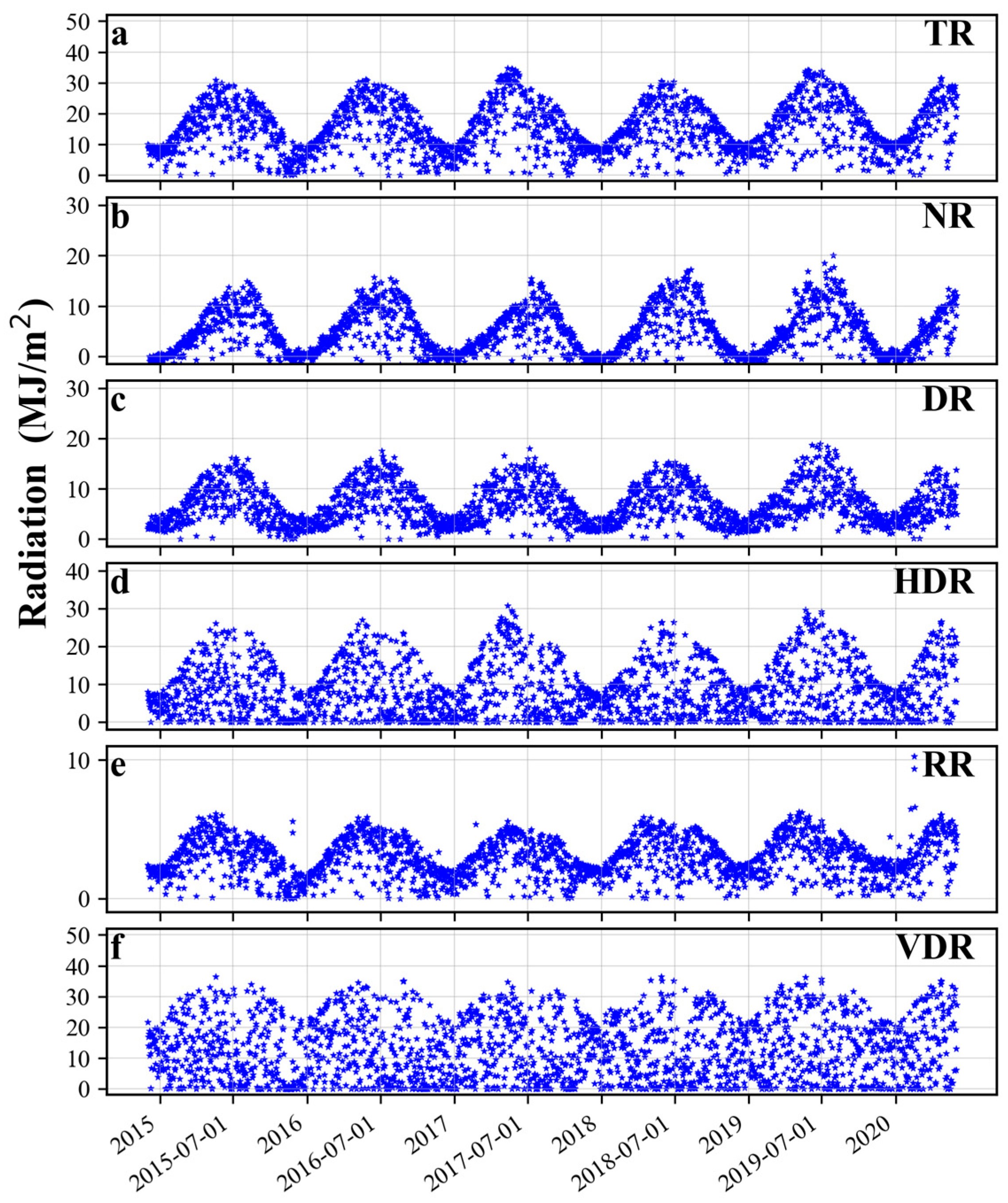
Daily surface solar radiation and meteorological conditions both show strong seasonal variability (Figure A1, Figure A2, Figure A3, Figure A4, Figure A5 and Figure A6). This shared seasonality is expected because solar geometry dominates the annual cycle, while meteorology modulates the amount and partitioning of radiation reaching the surface. To clarify how meteorological variability relates to radiation components at different time scales, and how these relationships change with pollution level, we first examined time–frequency coherence and then summarized pollution-dependent statistical relationships.

3.1.1. Relationship Between Surface Solar Radiation and Cloud Cover

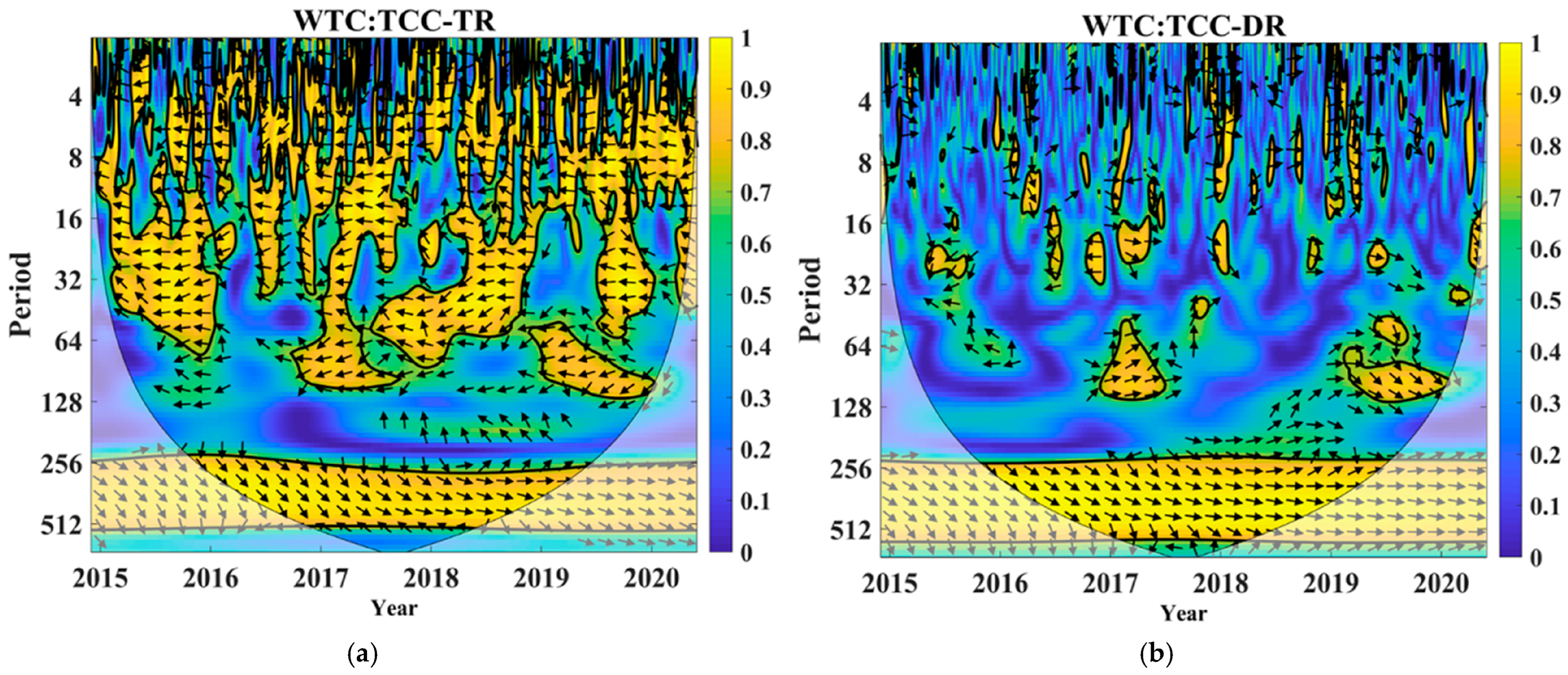
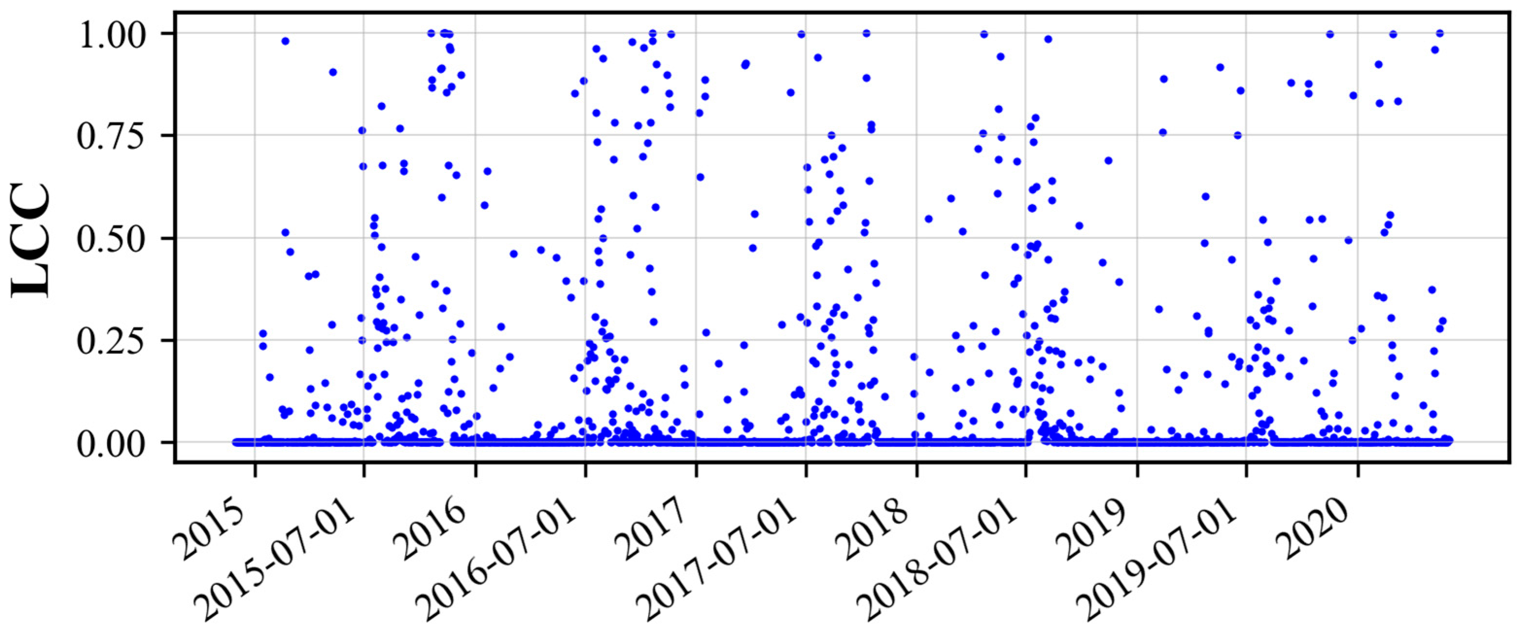
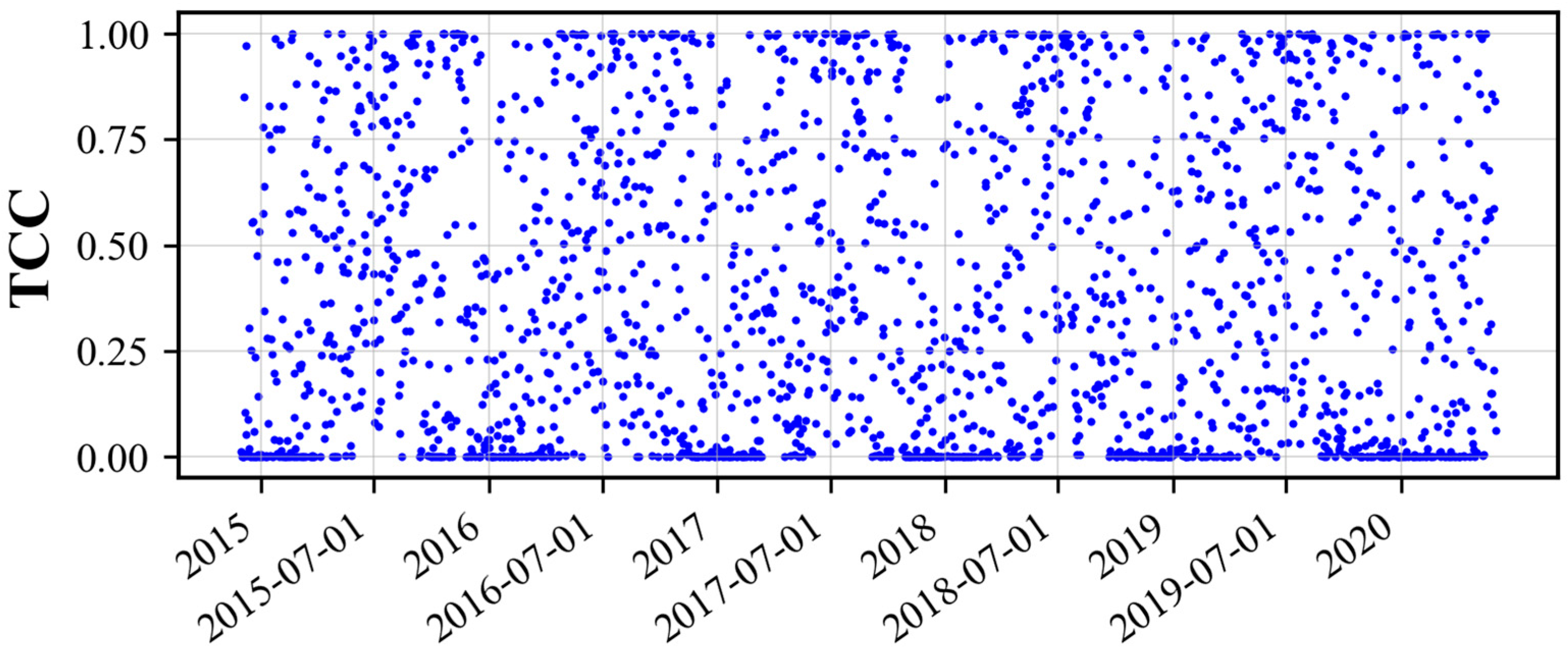
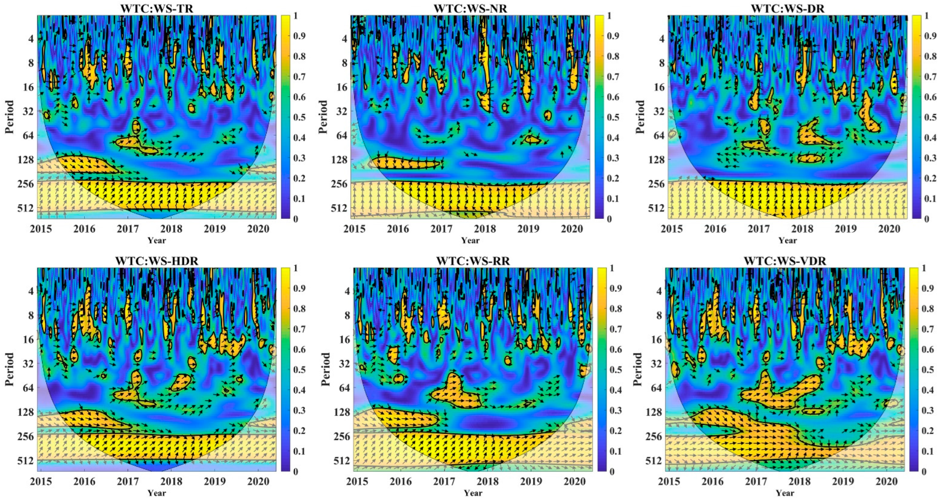
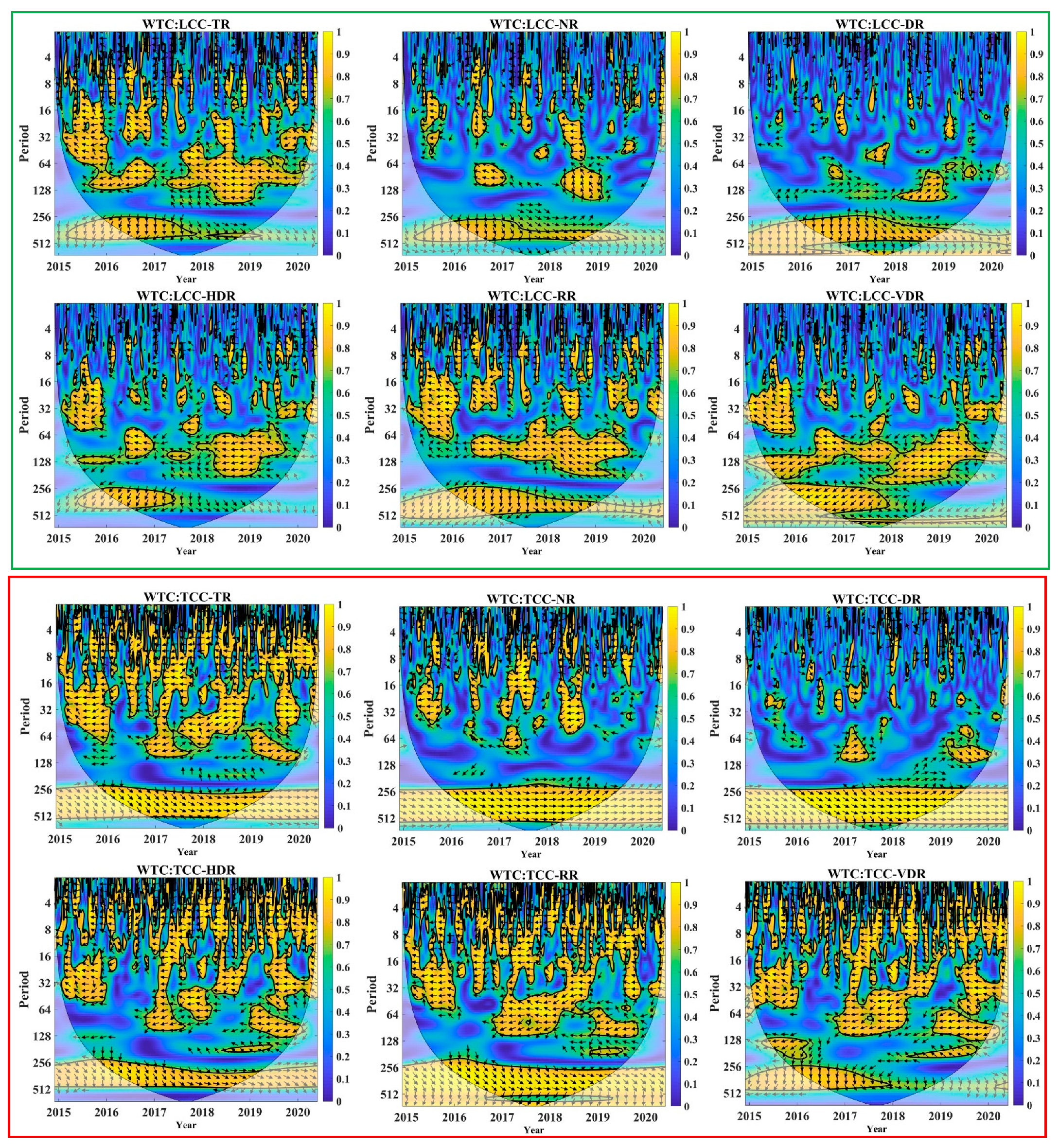
Meteorological factors, like radiation components, show clear seasonal variability. In this study, the wavelet transform coherence (WTC) results indicate persistent annual-scale coherence (256–512 d band, p < 0.05) between total cloud cover (TCC) and the radiation components. Low cloud cover (LCC) shows a phase lead of about 90° relative to the radiation components in the same annual band, consistent with the seasonal evolution in the corresponding time series (Figure A1, Figure A2 and Figure A3). The annual coherence mainly reflects shared seasonality, while the phase relationship suggests that cloud cover and radiation components do not vary in perfect synchrony.
Cloud cover is also linked to sub-seasonal fluctuations in surface radiation. At shorter time scales, cloud variability is predominantly associated with reduced surface radiation, and this negative coherence is most evident for total radiation and several direct components (Figure 1). For DR, coherence is weaker and can vary across time–frequency regions. Similar time–frequency patterns are observed for other radiation components and for LCC/TCC in the complete WTC panels (Figure A11).

3.1.2. Relationship Between Surface Solar Radiation and Water Vapour

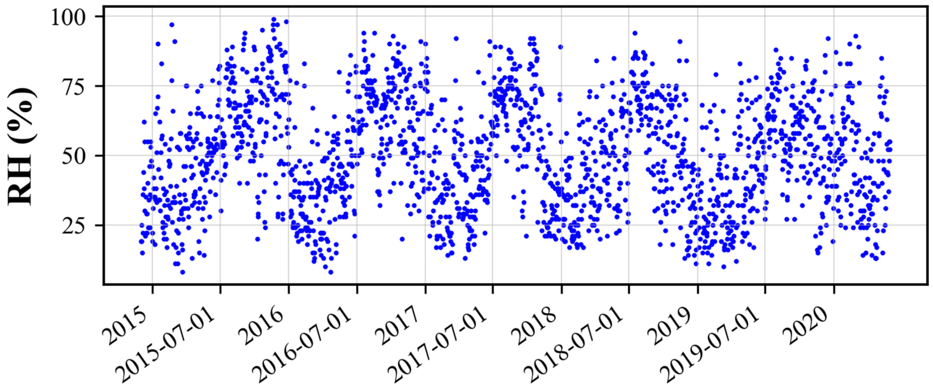
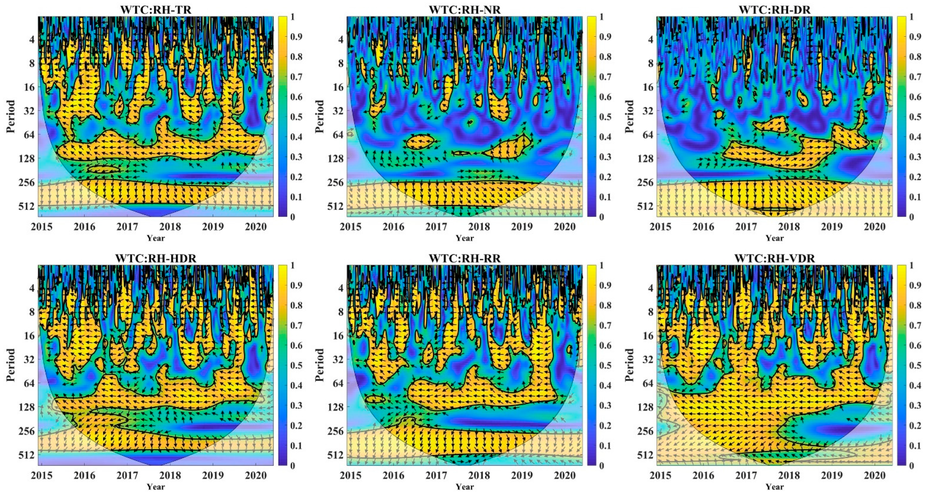
Relative humidity (RH), which is used here as a proxy for water-vapor-related atmospheric conditions [19], shows significant coherence with radiation components, particularly in the annual band (256–512 days, p < 0.05). The phase difference between RH and the radiation signals is approximately 90°, which is consistent with the seasonal timing of the two series (Figure A1 and Figure A4). Compared with cloud cover, RH shows a different phase relationship with radiation, reflecting a different pattern of seasonal covariation. At shorter time scales (64–128 days), RH shows stronger coherence with DR, while its correlation with TR and other radiation components is generally negative (Figure A12).

3.1.3. Relationship Between Surface Solar Radiation and Other Meteorological Factors

Surface temperature and near-surface air temperature are tightly controlled by the surface radiation budget on seasonal time scales, and as such, temperature variables are not the focus of this study [63,64]. Wind direction is also excluded, as its interpretation involves complex transport pathways and source regions, which lie beyond the scope of this analysis. Instead, we focus on pressure (P), the vertical integral of atmospheric mass (VMA), wind speed (WS), and precipitation (PRE), which are commonly used in meteorology and air quality studies to represent synoptic conditions.
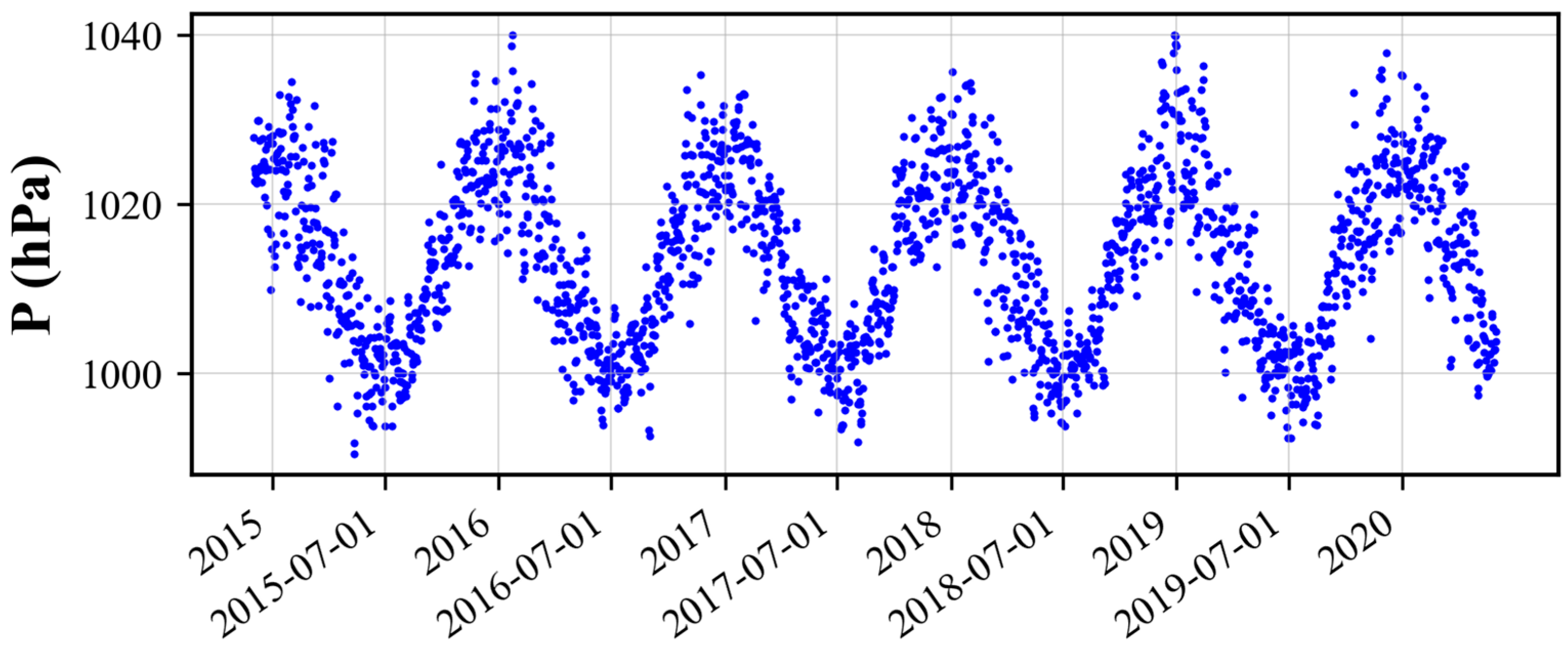
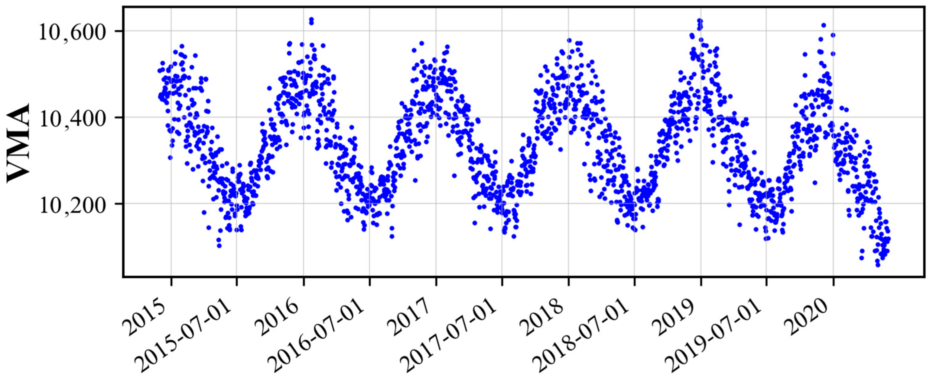
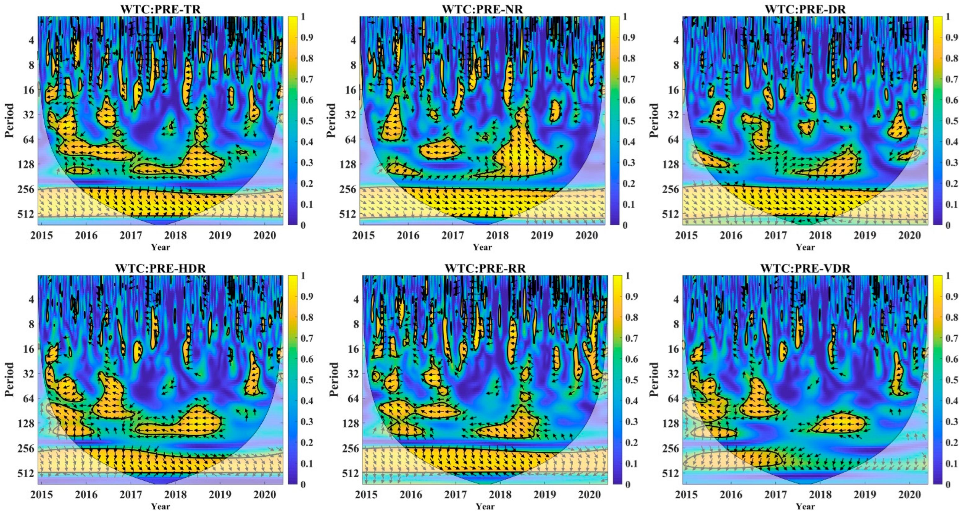
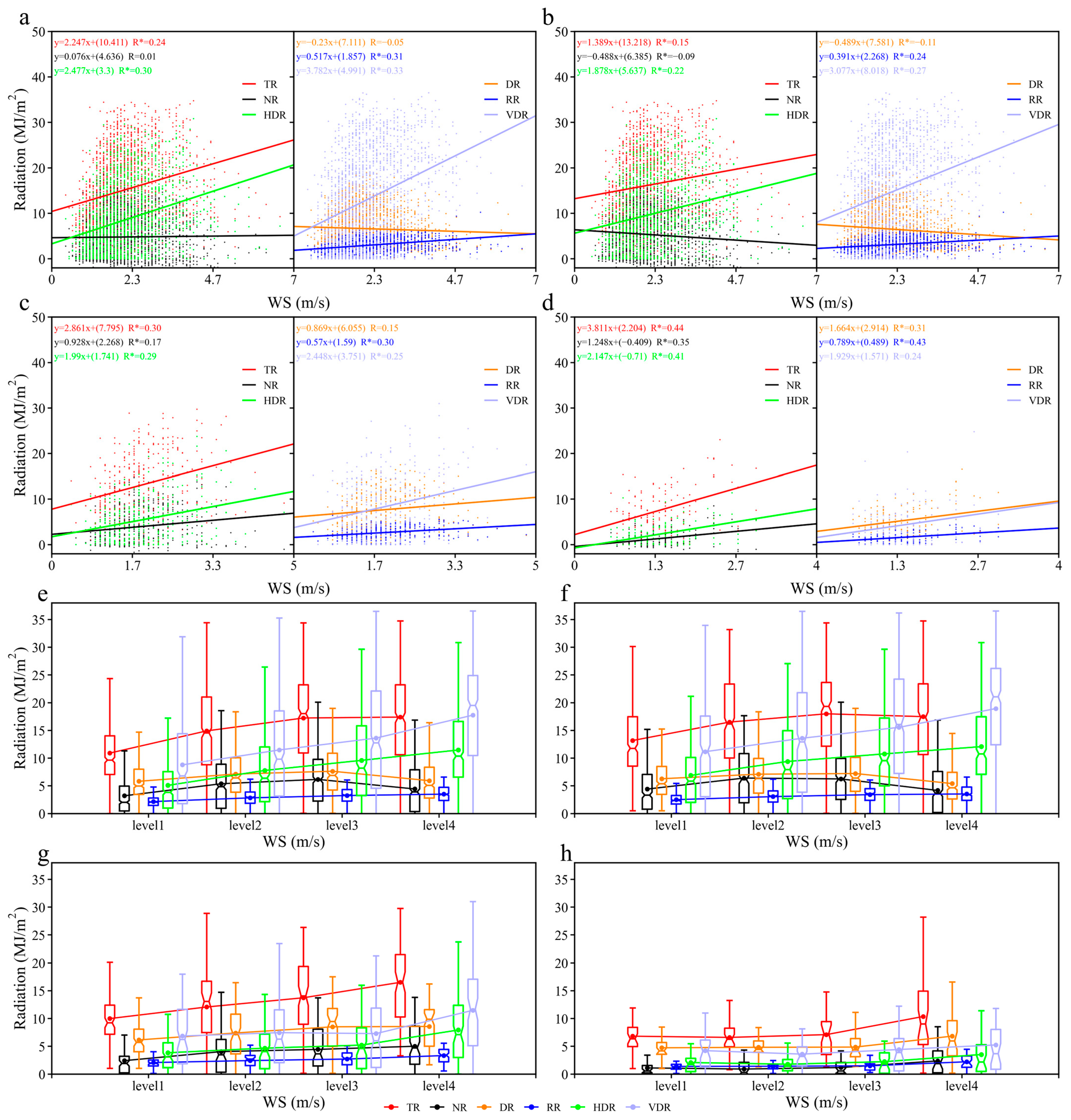
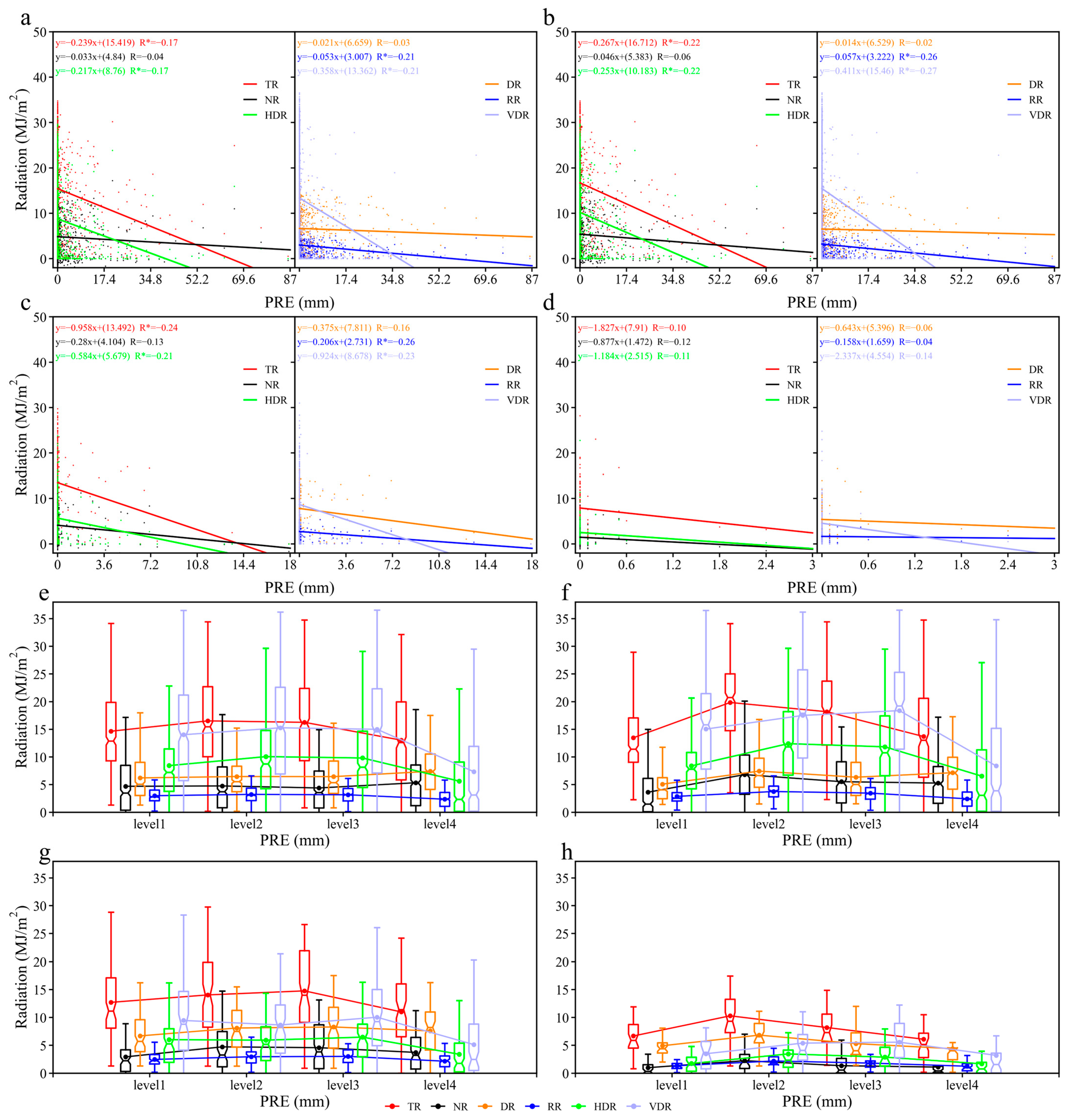
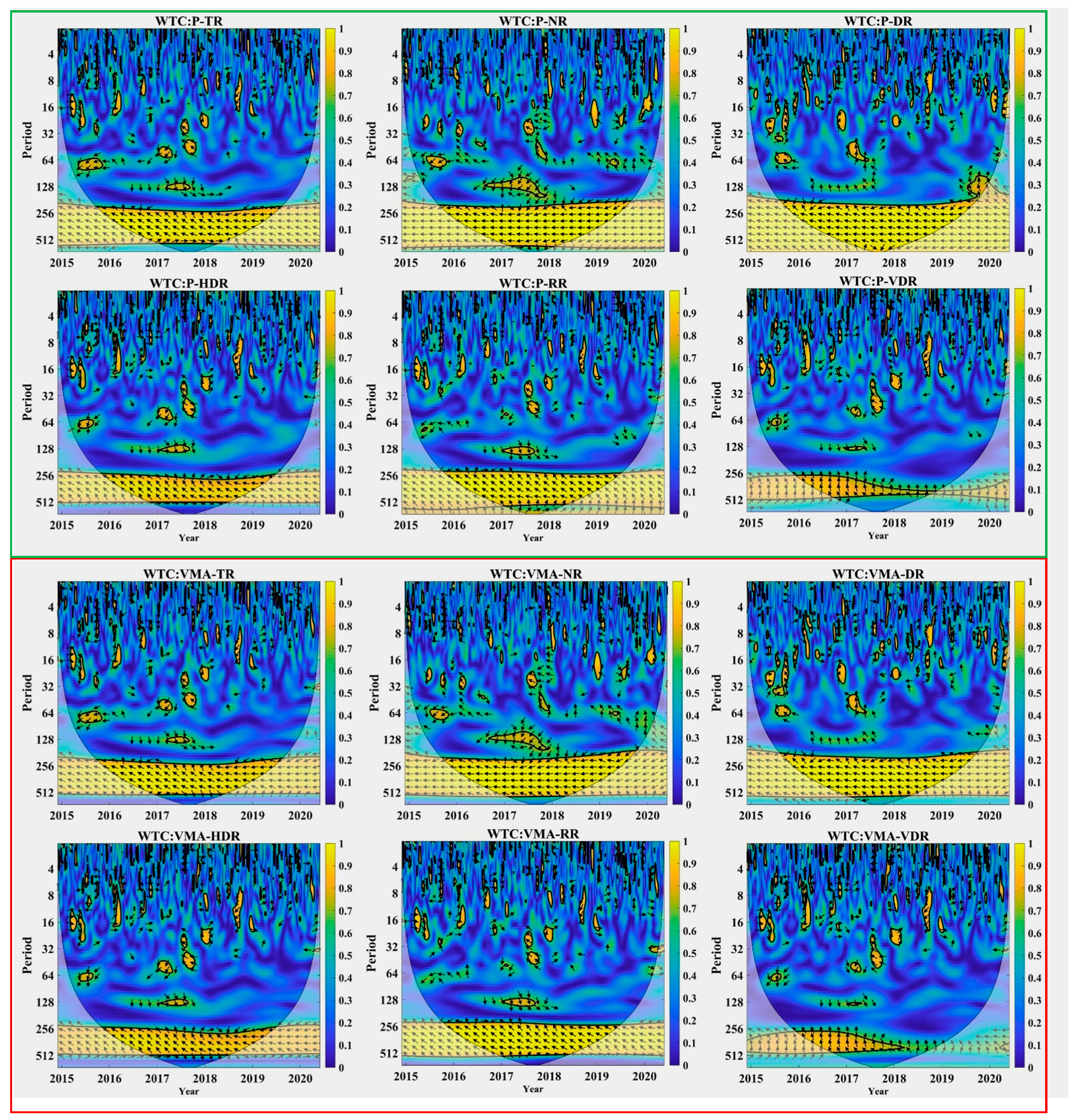
The wavelet transform coherence (WTC) results indicate that P is strongly coherent with radiation components at the annual scale (256–512 days, p < 0.05), with a phase relationship suggesting that p varies out of phase with the annual radiation cycle (Figure A1 and Figure A5). Coherence between P and radiation components at shorter time scales is weak and inconsistent, indicating that the relationship is primarily driven by seasonal variations. VMA shows a similar time–frequency pattern to P, reflecting the close correspondence between their time series (Figure A5 and Figure A6), with their WTC results summarized in Figure A13. WS and PRE show significant coherence with radiation components at the annual scale (Figure A7 and Figure A8), though their coherence at shorter time scales is intermittent, consistent with the episodic nature of weather regimes and event-scale variability.

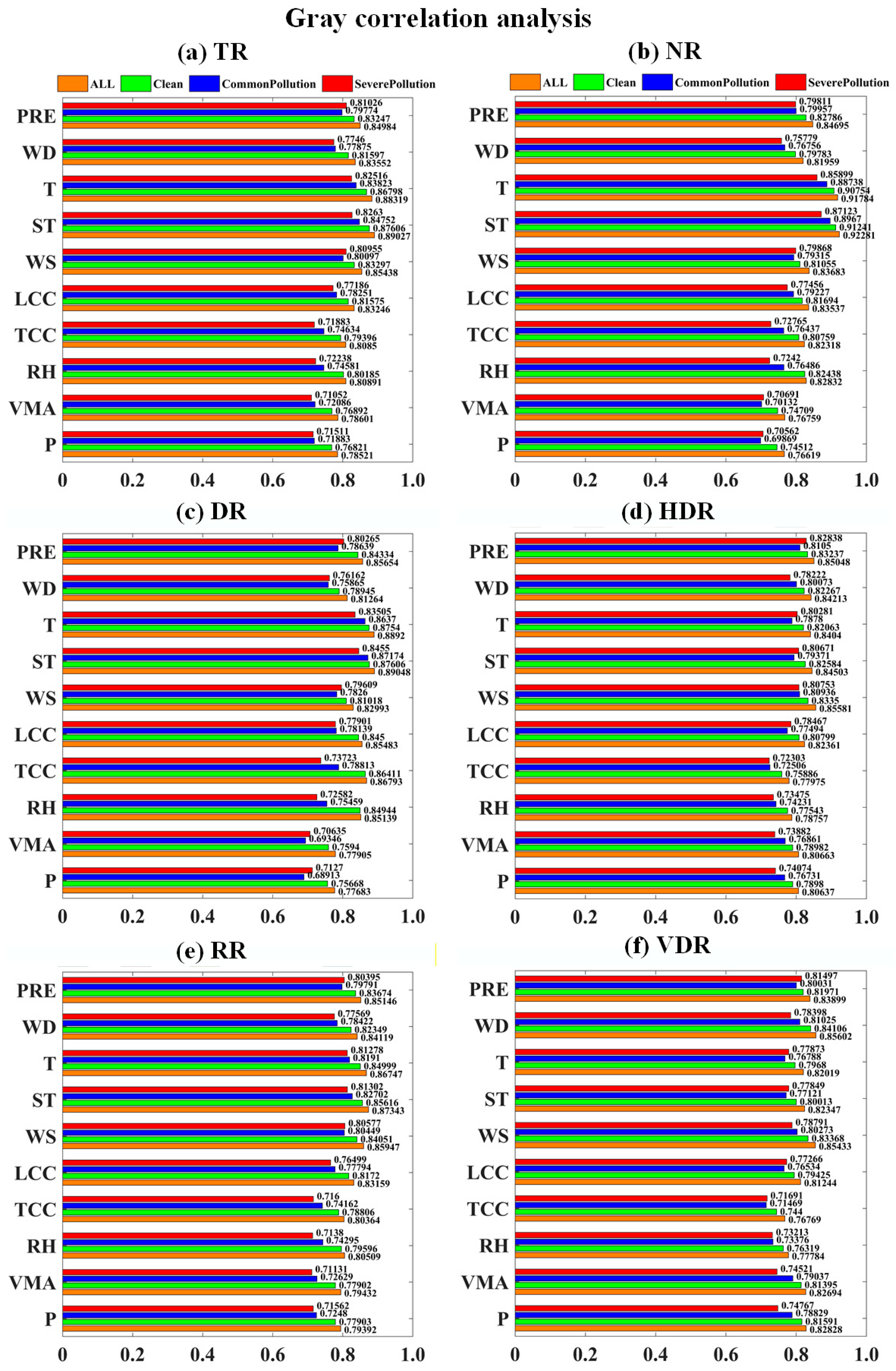
3.1.4. Gray Correlation Analysis Under Different Pollution Levels

Figure 2 summarizes gray relational coefficients between meteorological factors and radiation components under different pollution levels. When all days are pooled, the coefficients tend to be higher, but stratifying by pollution level reduces these values and increases variability across the factors. Second, the relative ranking of factors is not identical across radiation components: direct-related components (e.g., HDR, RR, and VDR) often show stronger alignment with cloud-related variability, whereas components that depend more on partitioning (notably DR, panel c) show a more mixed pattern and a clearer sensitivity to the pollution stratification. Third, moving from clean to severe pollution, the set of factors with relatively high coefficients tends to become more variable, suggesting that daily radiation variability is influenced by a broader combination of co-varying conditions under heavier pollution regimes.

3.2. Pollution-Dependent Statistical Relationships

Meteorological factors significantly affect daily radiation components, and these relationships change depending on pollution levels. We focus on cloud cover and relative humidity (RH), as they are consistently related to radiation variability. To reduce the impact of outliers and better capture non-linearities at the daily scale, we use binned statistics to summarize the relationships. For each pollution category, the cloud-cover and RH data were divided into four quantile-based bins (levels 1–4) from low to high values, and the corresponding mean radiation responses were calculated within each bin.

3.2.1. Cloud Cover

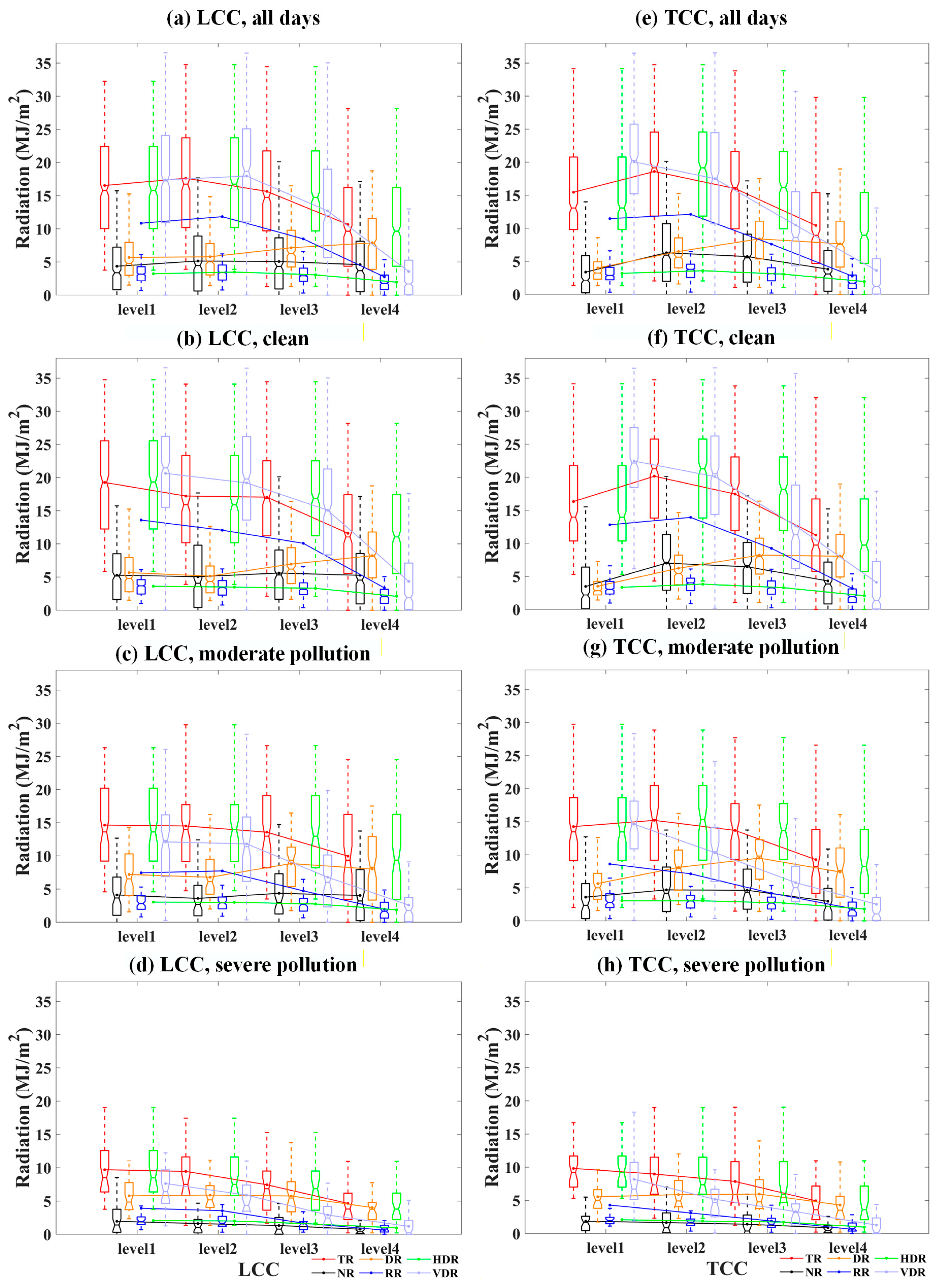
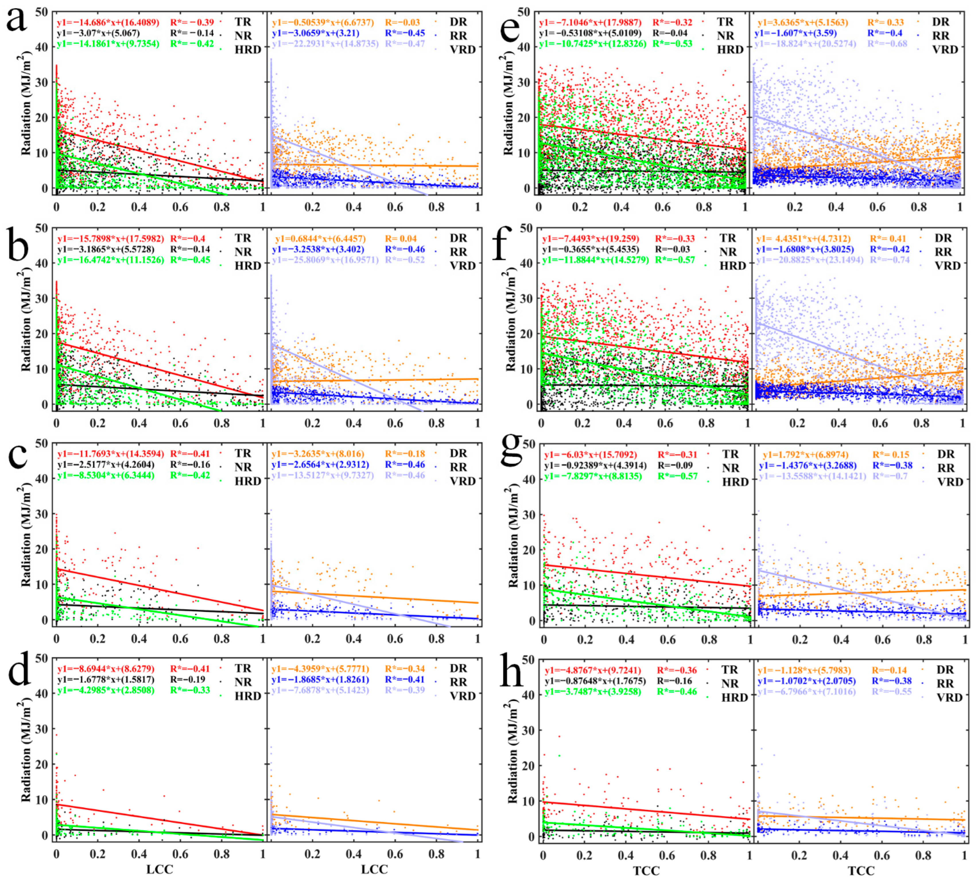
Figure 3 shows how radiation components change with different levels of cloud cover under varying pollution conditions. In general, as cloud cover increases, TR, NR, HDR, RR, and VDR decrease, which aligns with the expected attenuation of solar radiation by clouds. However, DR behaves differently: it initially increases with low-to-moderate cloud cover, then decreases as cloud cover becomes more extensive. The cloud–radiation relationship also changes with pollution levels. As pollution increases, the rate of decrease in TR, NR, HDR, RR, and VDR with more cloud cover becomes smaller. DR’s response weakens under higher pollution. Scatter correlations provide further support for this pattern (Figure A14). Figure 3 shows the pooled daily relationships between cloud cover and radiation components across 2015–2019 under different pollution conditions.

3.2.2. Relative Humidity (RH)

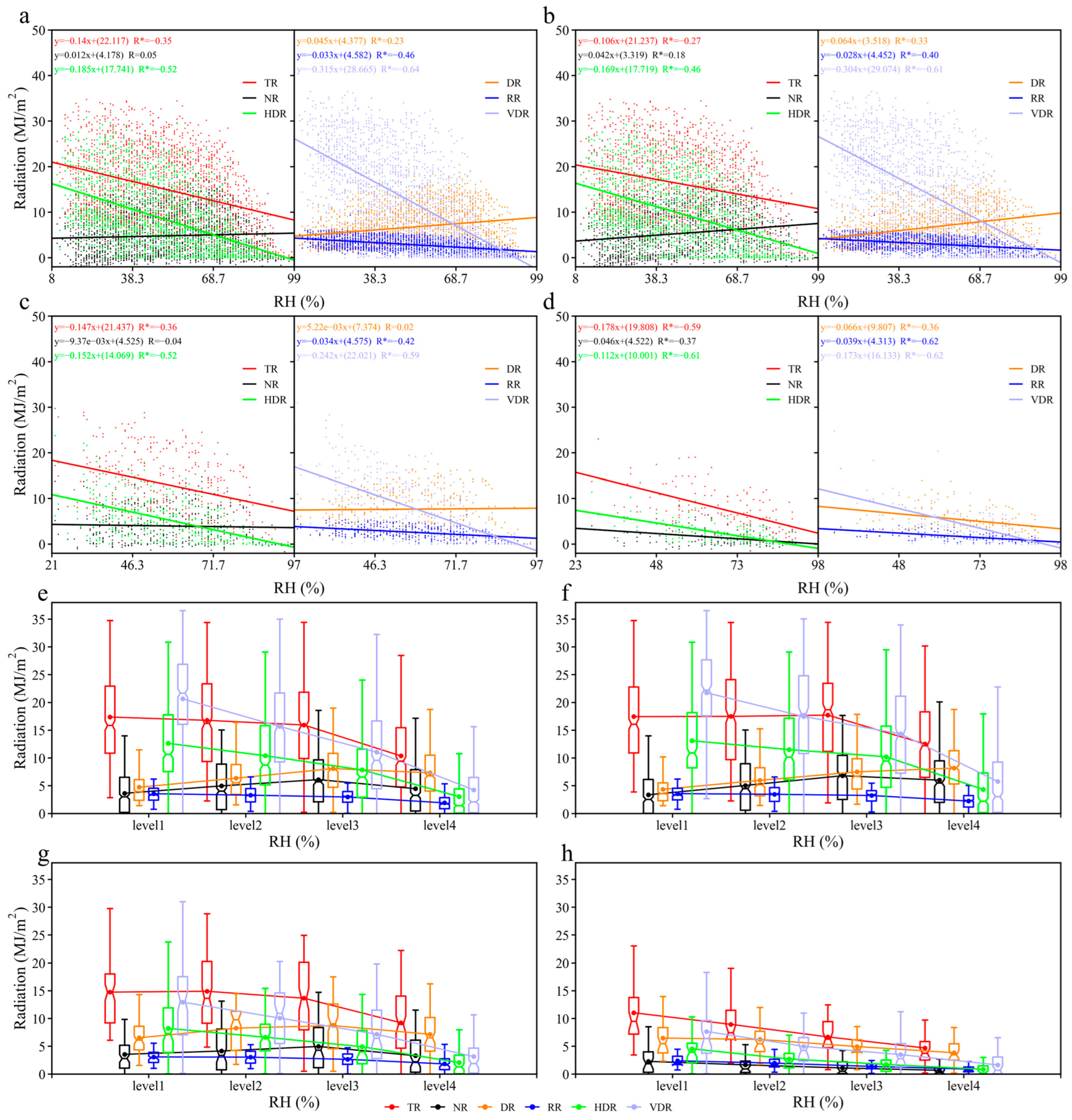
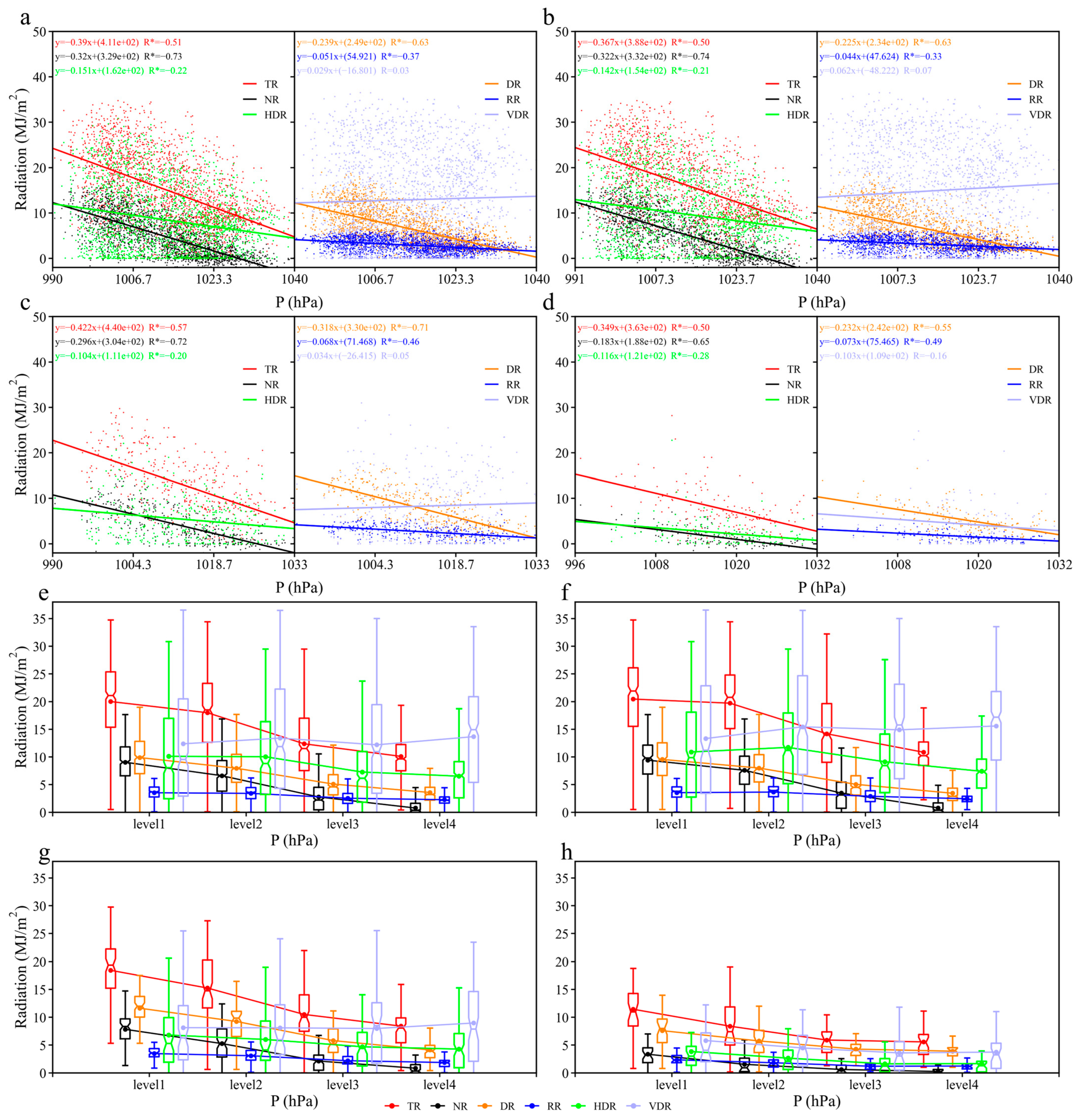
Figure 4 summarizes RH–radiation relationships under different pollution conditions. In this study, the association between RH and most radiation components (except DR) becomes more negative as pollution increases. The binned results further show that under severe pollution, radiation components decrease more rapidly with increasing RH, indicating a stronger humidity dependence in heavily polluted conditions.
DR shows the clearest pollution dependence. Under cleaner conditions, DR can be positively associated with RH, whereas under severe pollution the relationship becomes negative (Figure 4). Another notable feature in Figure 4 is the sensitivity of direct components, especially VDR, to RH under higher pollution. Overall, the RH stratification shows that meteorological–radiation relationships vary systematically with pollution level.

3.3. Comparison of Meteorological Normalization Results (MLR vs. RF)

In Section 3.1 and Section 3.2, we demonstrated that daily radiation components are significantly influenced by meteorological variability, with these relationships varying across different pollution levels. To further evaluate this variability, we compared the anomaly-based MLR results with deseasonalized/detrended anomalies derived from the RF-normalized daily radiation series.
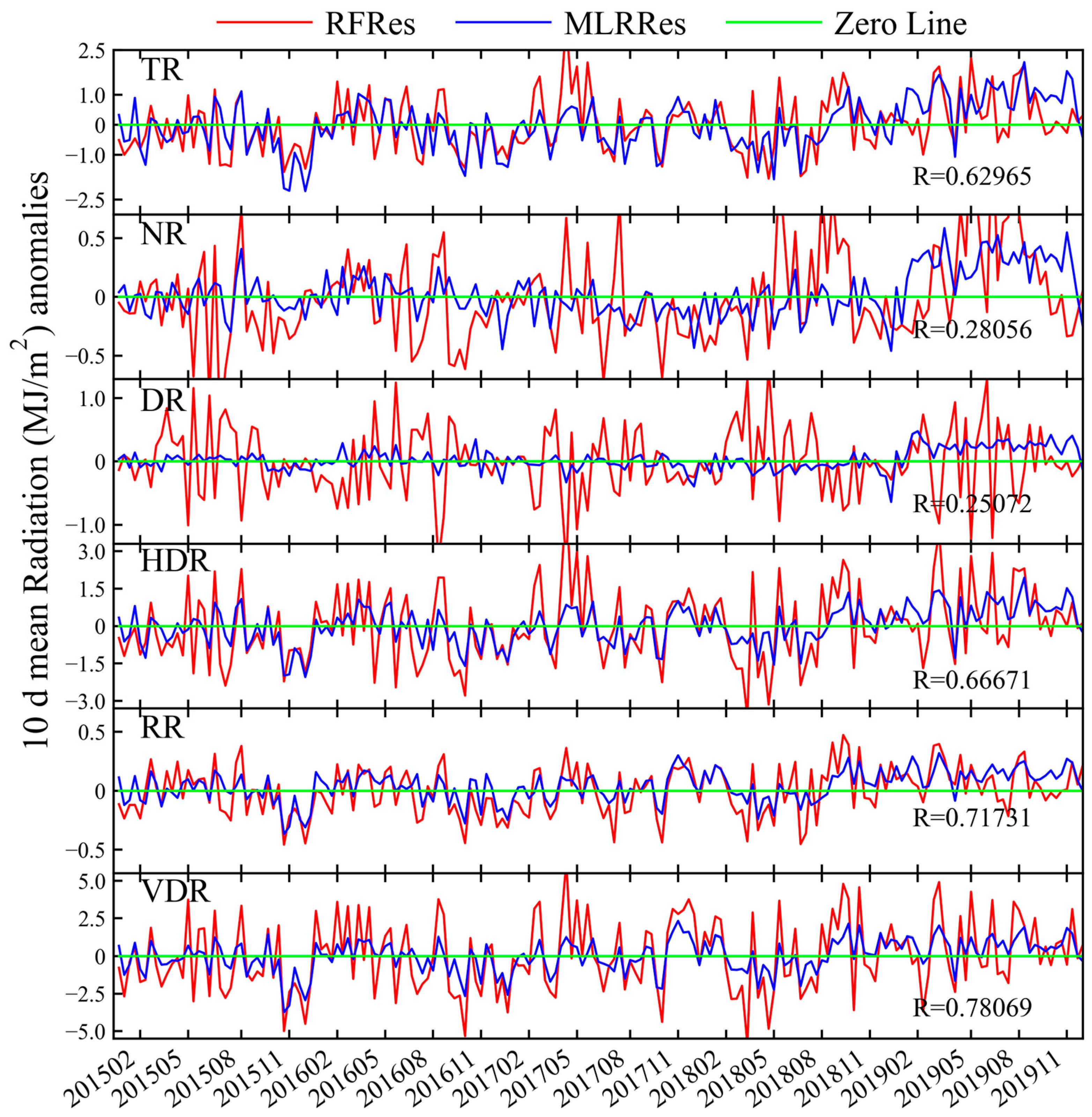
The performance of the MLR model for each radiation component is summarized in Table 2. While MLR provides a good fit for most components, it performs less effectively for NR and DR. Figure 5 compares the 10-day mean meteorologically adjusted anomalies from both RF and MLR methods. Despite some differences in amplitude, both methods show similar temporal variations in radiation components, with trend correlations ranging from 0.63 to 0.78. RF-adjusted anomalies exhibit somewhat larger variability.

4. Discussion

4.1. Pollution-Dependent Shifts in Meteorological–Radiation Relationships

The results show that the relationships between meteorological factors and surface solar radiation components are not fixed, but vary systematically with pollution level. This feature is evident in both the gray relational analysis and the pollution-stratified statistical results. When all days are pooled, several meteorological factors show relatively strong and stable associations with radiation components. After stratification by pollution level, however, these associations become less uniform, and the dominant factors vary more clearly among radiation components and pollution regimes. This indicates that daily radiation variability is influenced by a broader and more coupled set of atmospheric conditions under polluted environments. Such behavior is consistent with the influence of multiple co-varying factors and their coupled effects under polluted conditions [65,66].
A similar pattern is evident in the cloud-cover and RH analyses. For cloud cover, the attenuation of TR, NR, HDR, RR, and VDR becomes weaker as pollution increases, suggesting that the apparent cloud sensitivity of these components is modified under polluted conditions. For RH, the relationships with most radiation components become more negative as pollution increases, and under severe pollution the radiation components decrease more rapidly with increasing RH. Taken together, these results suggest that pollution does not simply add an independent perturbation to the radiation field. Instead, it changes the apparent response of radiation components to meteorological variability, likely because cloud, humidity, visibility, aerosol loading, and boundary-layer conditions co-vary more strongly when the atmosphere is polluted [65,66].
These results help explain why daily radiation–pollution relationships are difficult to interpret directly from observed time series. At the daily scale, the measured response of radiation to pollution is strongly entangled with simultaneous meteorological variability. As a result, differences in apparent radiation sensitivity across pollution levels should not be interpreted only as direct aerosol radiative effects, but rather as the combined outcome of co-varying atmospheric conditions. This also indicates why meteorological normalization is necessary when radiation data are used to infer pollution-related variability.

4.2. Distinct Behavior of Diffuse Radiation Under Polluted Conditions

Among all radiation components, DR shows the clearest pollution-dependent behavior. In the cloud-cover analysis, DR first increases under low-to-moderate cloud conditions and then decreases when cloud cover becomes more extensive. In the RH analysis, DR is positively associated with RH under cleaner conditions but becomes negatively associated with RH under severe pollution. These patterns differ from those of the direct-related components and indicate that DR responds to atmospheric variability through mechanisms that are more complex than simple attenuation. The cloud-related behavior of DR is consistent with previous studies showing that diffuse radiation can vary nonlinearly with cloud fraction and cloud regime [67].
It means DR depends strongly on the partitioning between direct and diffuse radiation, which is sensitive to both cloud scattering and aerosol-related extinction. Under relatively clean conditions, increasing cloud cover or RH can enhance scattering and therefore increase the diffuse fraction, even when the total incoming shortwave radiation does not increase. Under polluted and humid conditions, however, aerosol hygroscopic growth and enhanced extinction may reduce the transmitted radiation more strongly, so that even DR declines. This also indicates that the response of DR reflects not only cloud amount or humidity itself, but also how these factors interact with aerosol optical properties and atmospheric transmissivity [68,69,70,71].
This distinct behavior of DR is important because it shows that different radiation components should not be interpreted in the same way when evaluating pollution-related variability. Direct related components mainly reflect attenuation of the transmitted beam, whereas DR reflects redistribution within the radiation field and is therefore more sensitive to coupled cloud–aerosol–humidity effects. The stronger pollution dependence of DR in this study further distinguishes it from the other radiation components and is consistent with a more complex response involving multiple coupled atmospheric processes that are not fully resolved at the daily scale.

4.3. Implications for Meteorological Normalization: MLR Versus RF

The comparison between MLR- and RF-based normalization shows that the two approaches produce broadly consistent temporal variations in meteorologically adjusted anomalies, despite differences in amplitude. This agreement is important because it indicates that the main daily-scale signals are not an artifact of one specific adjustment method. At the same time, RF generally shows stronger predictive performance for the original daily radiation components, while MLR performs less well for some components, especially NR and DR. This difference is expected because RF is better able to capture nonlinear responses and interactions among predictors.
The consistency between the two approaches supports the practical value of RF-based normalization for daily station radiation records. In particular, RF provides a flexible framework for adjusting for meteorological variability without requiring a strictly linear relationship between predictors and radiation components. This is useful under polluted conditions, where cloud, humidity, and aerosol-related variables may interact in ways that are difficult to represent with linear models alone. The present results therefore support the use of RF as a practical meteorological–normalization tool for daily radiation analysis, especially when the objective is to isolate meteorologically adjusted variability rather than to derive an explicit process-based attribution.
At the same time, the comparison also highlights an important methodological distinction. In this study, the RF model was trained on absolute daily radiation components and then used to generate normalized daily radiation series, which were subsequently deseasonalized and detrended for comparison with the anomaly-based MLR results. The two methods are therefore comparable at the level of adjusted variability, but they are not identical in formulation. Overall, the agreement between the two approaches reinforces the value of meteorological normalization for characterizing daily radiation variability under different pollution conditions, while also indicating that the adjusted signals remain sensitive to methodological choices.

5. Conclusions

In this study, we analyzed daily surface solar radiation components and meteorological conditions at the Beijing 54511 station during the period of 2015–2019 to assess how meteorological variability relates to radiation under different pollution levels. We combined wavelet transform coherence and gray relational analysis with stratified statistics, and we further compared meteorological normalization results from multiple linear regression (MLR) and a random-forest (RF) approach.
The results show that cloud cover and relative humidity (RH) are consistently associated with variability in radiation components across multiple time scales, with particularly strong coherence at the annual band. Gray relational analysis further shows that the relative strength of meteorological associations differs among radiation components and becomes less uniform after stratification by pollution level, especially under severe pollution.
Pollution-stratified statistics show that meteorological–radiation relationships depend on pollution level. With increasing pollution, the apparent sensitivity of several radiation components to cloud cover weakens, while the association between RH and most radiation components becomes more negative. DR exhibits the most distinct behavior, with a clear pollution-dependent shift in its RH relationship.
The comparison between MLR- and RF-based meteorological normalization shows broadly consistent temporal variations in adjusted radiation anomalies across components, with trend correlations of 0.63–0.78. Together with the stronger predictive performance of RF (R2 = 0.83–0.88 in Table 1), this comparison supports the practical use of RF-based meteorological normalization for daily radiation analysis. For components with weaker MLR fits, especially NR and DR, the adjusted anomalies remain less certain.
Overall, the findings highlight the importance of explicitly accounting for meteorological variability when interpreting daily radiation–pollution relationships. Future work using hourly or finer-resolution observations, together with more explicit constraints on solar-position effects and cloud conditions, would help provide a more physically constrained interpretation while retaining the practical value of meteorological normalization.

Author Contributions

Z.L. and T.W. determined the main goal of this study. T.W. carried out the study, analyzed the data, and prepared the paper with contributions from all co-authors. Z.L. provided guidance on data processing methods and improvement of the content of the article and made suggestions on grammatical issues and graphic formatting issues in the article. X.Z. provided advice on data processing code writing and plotting. Z.L. and T.W. helped modify the grammar of the article and polished the language. All authors have read and agreed to the published version of the manuscript.

Funding

This work was supported by the Sichuan International Science and Technology Innovation Cooperation Project/Hong Kong, Macao, and Taiwan Science and Technology Innovation Cooperation Project (Grant No. 2026YFHZ0028), the Natural Science Foundation of China (NSFC) research project (Grant No. 42501431 and 42405085) and the Fundamental Research Funds for the Central Universities (Grant No. PHD2023-022 and 25CAFUC04032).

Data Availability Statement

The raw data supporting the conclusions of this article will be made available by the authors upon request.

Conflicts of Interest

The authors declare no conflicts of interest.

Appendix A

Figure A1. Time series of solar radiation components during the core analysis period (2015–2019): (a) total radiation (TR); (b) net radiation (NR); (c) diffuse radiation (DR); (d) horizontal direct solar radiation (HDR); (e) reflected radiation (RR); (f) vertical direct solar radiation (VDR).
Remotesensing 18 01368 g0a1
Figure A2. Time series of LCC during the core analysis period (2015–2019).
Remotesensing 18 01368 g0a2
Figure A3. Time series of TCC during the core analysis period (2015–2019).
Remotesensing 18 01368 g0a3
Figure A4. Time series of RH during the core analysis period (2015–2019).
Remotesensing 18 01368 g0a4
Figure A5. Time series of P during the core analysis period (2015–2019).
Remotesensing 18 01368 g0a5
Figure A6. Time series of VMA during the core analysis period (2015–2019). (Vertical integral of mass of atmosphere is the total mass of air for a column extending from the surface of the Earth to the top of the atmosphere, per square meter).
Remotesensing 18 01368 g0a6
Figure A7. Wavelet coherence between surface solar radiation and wind speed. The black contour lines show the regions of power significant at the 5% level, which are computed based on 1000 Monte Carlo simulations. The cone of influence (black curve) indicates the region without edge effects. The power values are coded from dark blue for low power to v for high power, as shown in the right panel. The vectors indicate the phase difference between the WS and each radiation component: →: in phase; ←: in anti-phase; ↓: X leading Y by 90°; ↑: Y leading X by 90°.
Remotesensing 18 01368 g0a7
Figure A8. Wavelet coherence between surface solar radiation and precipitation. The black contour lines show the regions of power significant at the 5% level, which are computed based on 1000 Monte Carlo simulations. The cone of influence (black curve) indicates the region without edge effects. The power values are coded from dark blue for low power to bright yellow for high power, as shown in the right panel. The vectors indicate the phase difference between the PRE and each radiation component: →: in phase; ←: in anti-phase; ↓: X leading Y by 90°; ↑: Y leading X by 90°.
Remotesensing 18 01368 g0a8
Figure A9. Statistical relationship between wind speed and radiation components. (ad) represent the correlation between WS and radiation components under all, clean, common pollution and serious pollution respectively. An asterisk appended to the correlation coefficient indicates statistical significance at p < 0.001. The (eh) are the changes in radiation components with WS under all, clean, common pollution and serious pollution conditions respectively. Levels 1–4 represent the results of the classification of the last 4 samples of WS from small to large.
Remotesensing 18 01368 g0a9
Figure A10. Statistical relationship between precipitation and radiation components. (ad) represent the correlation between PRE and radiation components under all, clean, common pollution and serious pollution respectively. The correlation coefficient with asterisk indicates that its significance test is <0.001. (eh) show the changes in radiation components with PRE under all, clean, common pollution and serious pollution conditions respectively. Levels 1–4 represent the results of the classification of the last 4 samples of PRE from small to large.
Remotesensing 18 01368 g0a10
Figure A11. Wavelet transform coherence between surface solar radiation and cloud cover. The black contour lines show the regions of power significant at the 5% level, which are computed based on 1000 Monte Carlo simulations. The cone of influence (black curve) indicates the region without edge effects. The power values are coded from dark blue for low power to bright yellow for high power, as shown in the right panel. The vectors indicate the phase difference between the could cover and each radiation component: →: in phase; ←: in anti-phase; ↓: X leading Y by 90°; ↑: Y leading X by 90°. In the green and red boxes are the wavelet transform coherence of LCC, TCC and surface solar radiation, respectively.
Remotesensing 18 01368 g0a11
Figure A12. Wavelet coherence between surface solar radiation and water vapour. The black contour lines show the regions of power significant at the 5% level, which are computed based on 1000 Monte Carlo simulations. The cone of influence (black curve) indicates the region without edge effects. The power values are coded from dark blue for low power to bright yellow for high power, as shown in the right panel. The vectors indicate the phase difference between the RH and each radiation component: →: in phase; ←: in anti-phase; ↓: X leading Y by 90°; ↑: Y leading X by 90°.
Remotesensing 18 01368 g0a12
Figure A13. Wavelet coherence between atmospheric pressure, vertical integral of mass of atmosphere and surface solar radiation. The black contour lines show the regions of power significant at the 5% level, which are computed based on 1000 Monte Carlo simulations. The cone of influence (black curve) indicates the region without edge effects. The power values are coded from dark blue for low power to bright yellow for high power, as shown in the right panel. The vectors indicate the phase difference between the P or VMA and each radiation component: →: in phase; ←: in anti-phase; ↓: X leading Y by 90°; ↑: Y leading X by 90°. In the green and red boxes are the wavelet transform coherence of P, VMA and surface solar radiation, respectively.
Remotesensing 18 01368 g0a13
Figure A14. Scatter fitting results of the correlation between cloud cover and radiation components under different pollution concentrations. The correlation coefficient with asterisk indicates that its significance test is <0.001. (ad) represent the correlation between LCC and radiation components under all, clean, common pollution and serious pollution respectively. (eh) correspond to TCC.
Remotesensing 18 01368 g0a14
Figure A15. Statistical relationship between atmospheric pressure and radiation components. (ad) represent the correlation between P and radiation components under all, clean, common pollution and serious pollution respectively. The correlation coefficient with asterisk indicates that its significance test is <0.001. (eh) are the changes in radiation components with P under all, clean, common pollution and serious pollution conditions respectively. Levels 1–4 represent the results of the classification of the last 4 samples of P from small to large.
Remotesensing 18 01368 g0a15
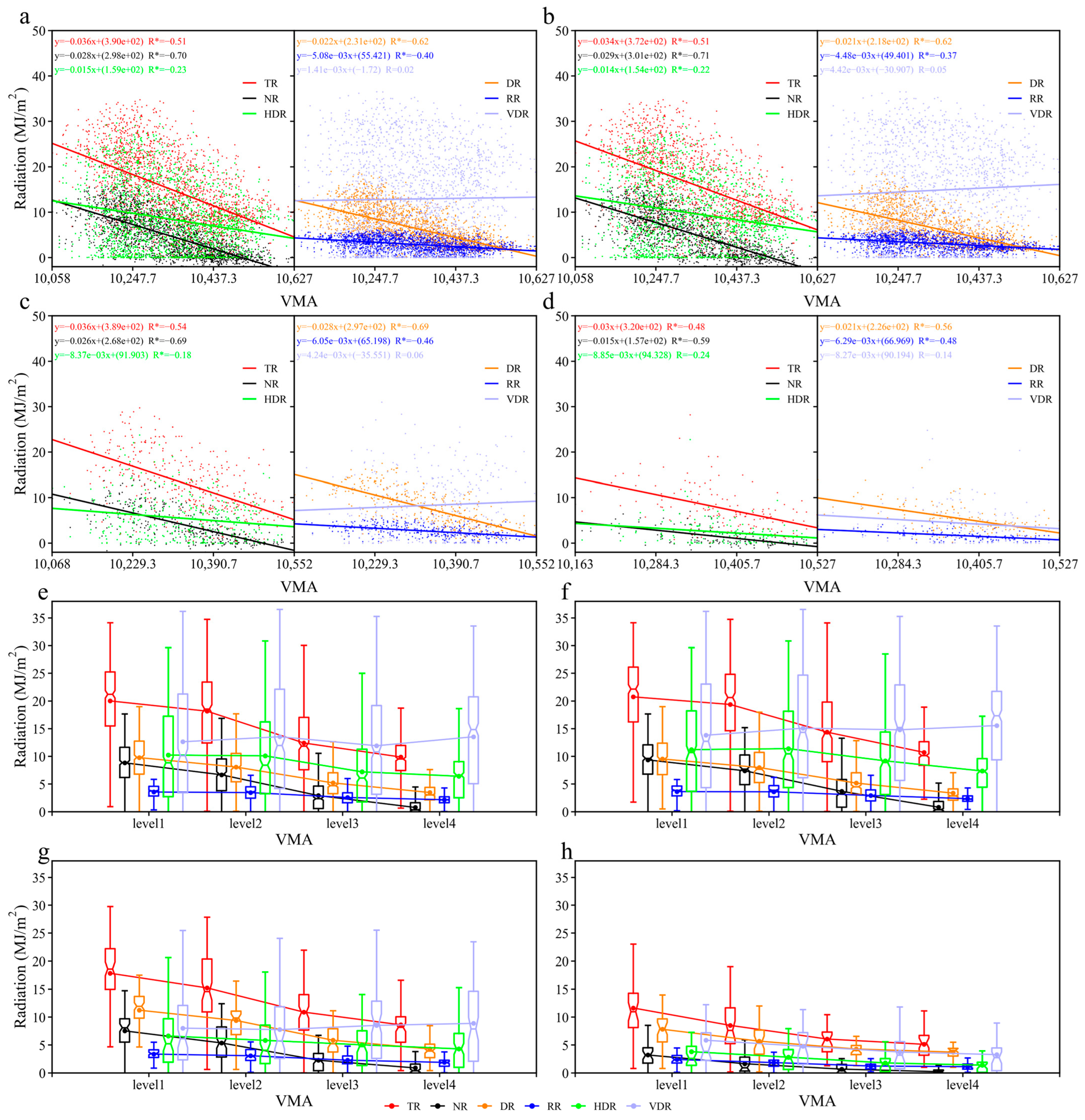
Figure A16. Statistical relationship between vertical integral of mass of atmosphere and radiation components. (ad) represent the correlation between VMA and radiation components under all, clean, common pollution and serious pollution respectively. The correlation coefficient with asterisk indicates that its significance test is <0.001. (eh) are the changes in radiation components with VMA under all, clean, common pollution and serious pollution conditions respectively. Levels 1–4 represent the results of the classification of the last 4 samples of VMA from small to large.
Remotesensing 18 01368 g0a16
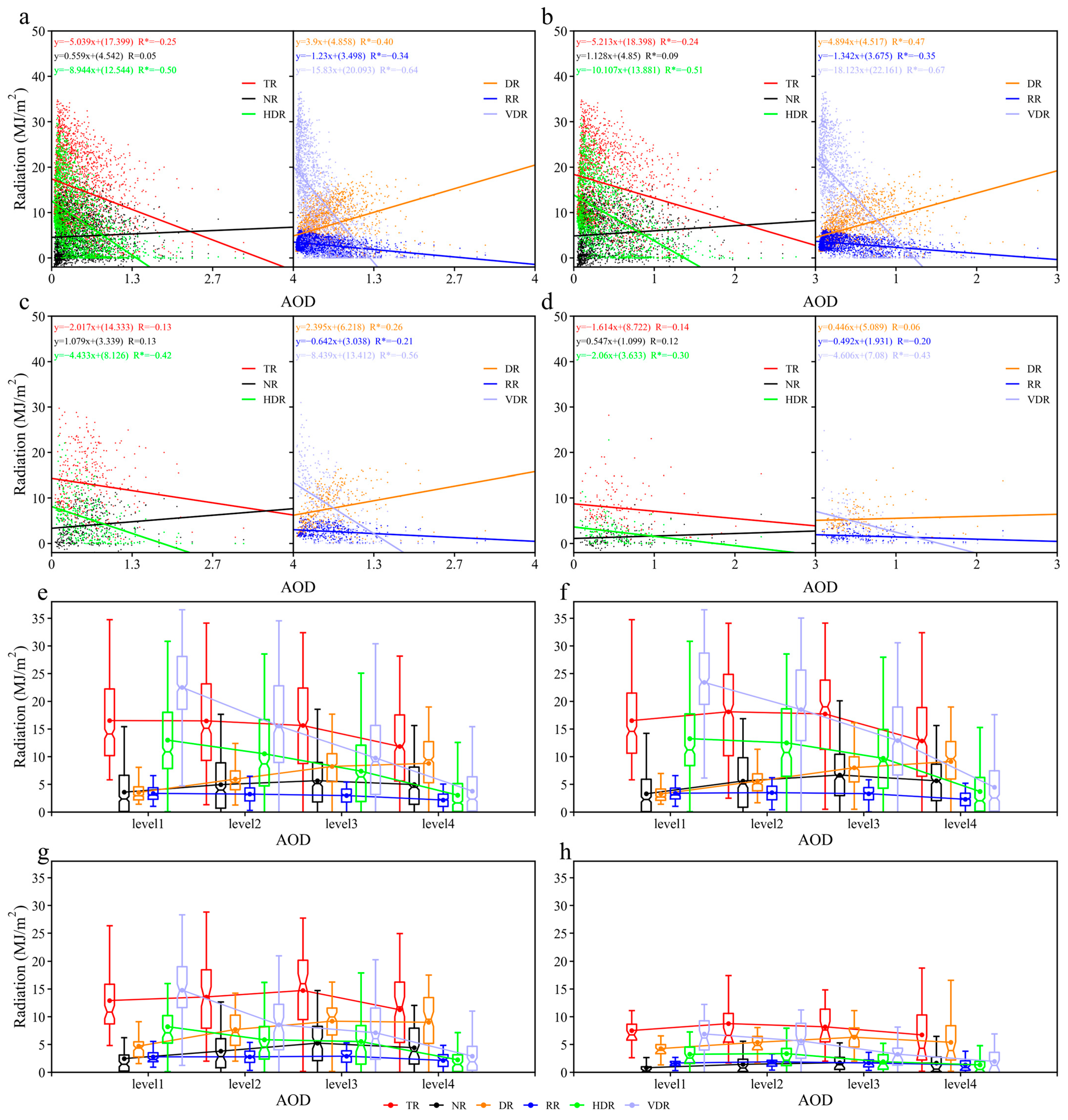
Figure A17. Statistical relationship between AOD and radiation components. (ad) represent the correlation between AOD and radiation components under all, clean, common pollution and serious pollution respectively. The correlation coefficient with asterisk indicates that its significance test is <0.001. (eh) are the changes in radiation components with AOD under all, clean, common pollution and serious pollution conditions respectively. Levels 1–4 represent the results of the classification of the last 4 samples of AOD from small to large.
Remotesensing 18 01368 g0a17

References

  1. Cline, D.W.; Bales, R.C.; Dozier, J. Estimating the spatial distribution of snow in mountain basins using remote sensing and energy balance modeling. Water Resour. Res. 1998, 34, 1275–1285. [Google Scholar] [CrossRef]
  2. Petra, K.K.; Katya, G.; Zbysek, M.; Michal, K.; Daniel, K.; Boian, K.; Katerina, P.; Josef, B. Solar signals detected within neutral atmospheric and ionospheric parameters. J. Atmos. Sol.-Terr. Phys. 2018, 171, 147–156. [Google Scholar] [CrossRef]
  3. Wild, M.; Folini, D.; Schaer, C.; Loeb, N.; Dutton, E.G.; Koenig-Langlo, G. The global energy balance from a surface perspective. Clim. Dyn. 2013, 40, 3107–3134. [Google Scholar] [CrossRef]
  4. Xu, J.; Zhong, K.; Wang, Y.; He, J.; Kang, Y. Influences of daily solar radiation intensity on the sea-land breeze and pollutant dispersion in coastal areas. Build. Environ. 2024, 258, 111600. [Google Scholar] [CrossRef]
  5. Mercado, L.M.; Bellouin, N.; Sitch, S.; Boucher, O.; Huntingford, C.; Wild, M.; Cox, P.M. Impact of changes in diffuse radiation on the global land carbon sink. Nature 2009, 458, 1014–1017. [Google Scholar] [CrossRef]
  6. Zhang, X.; Liang, S.; Wild, M.; Jiang, B. Analysis of surface incident shortwave radiation from four satellite products. Remote. Sens. Environ. 2015, 165, 186–202. [Google Scholar] [CrossRef]
  7. Kumar, R.; Umanand, L. Estimation of global radiation using clearness index model for sizing photovoltaic system. Renew. Energy 2005, 30, 2221–2233. [Google Scholar] [CrossRef]
  8. Ul Rehman Tahir, Z.; Hafeez, S.; Asim, M.; Amjad, M.; Farooq, M.; Azhar, M.; Murtza Amjad, G. Estimation of daily diffuse solar radiation from clearness index, sunshine duration and meteorological parameters for different climatic conditions. Sustain. Energy Technol. Assess. 2021, 47, 101544. [Google Scholar] [CrossRef]
  9. Wu, Y.; Eames, P.; Mallick, T.; Sabry, M. Experimental characterisation of a Fresnel lens photovoltaic concentrating system. Sol. Energy 2012, 86, 430–440. [Google Scholar] [CrossRef]
  10. Yang, X.F.; Qin, W.M.; Wang, L.C.; Zhang, M.; Niu, Z.G. Long-term variations of surface solar radiation in China from routine meteorological observations. Atmos. Res. 2021, 260, 105715. [Google Scholar] [CrossRef]
  11. Zhang, J.; Zhao, L.; Deng, S.; Xu, W.; Zhang, Y. A critical review of the models used to estimate solar radiation. Renew. Sustain. Energy Rev. 2017, 70, 314–329. [Google Scholar] [CrossRef]
  12. Lou, S.; Li, D.H.; Lam, J.C.; Chan, W.W. Prediction of diffuse solar irradiance using machine learning and multivariable regression. Appl. Energy 2016, 181, 367–374. [Google Scholar] [CrossRef]
  13. Haywood, J.M.; Bellouin, N.; Jones, A.; Boucher, O.; Wild, M.; Shine, K.P. The roles of aerosol, water vapor and cloud in future global dimming/brightening. J. Geophys. Res. Atmos. 2011, 116, D20203. [Google Scholar] [CrossRef]
  14. Seinfeld, J.H.; Bretherton, C.; Carslaw, K.S.; Coe, H.; DeMott, P.J.; Dunlea, E.J.; Feingold, G.; Ghan, S.; Guenther, A.B.; Kahn, R.; et al. Improving our fundamental understanding of the role of aerosol−cloud interactions in the climate system. Proc. Natl. Acad. Sci. USA 2016, 113, 5781–5790. [Google Scholar] [CrossRef]
  15. Chesnoiu, G.; Chiapello, I.; Ferlay, N.; Nabat, P.; Mallet, M.; Riffault, V. Regional modeling of surface solar radiation, aerosol, and cloud cover spatial variability and projections over northern France and Benelux. Atmos. Meas. Tech. 2025, 25, 1307–1331. [Google Scholar] [CrossRef]
  16. Papachristopoulou, K.; Fountoulakis, I.; Bais, A.F.; Psiloglou, B.E.; Papadimitriou, N.; Raptis, I.-P.; Kazantzidis, A.; Kontoes, C.; Hatzaki, M.; Kazadzis, S. Effects of clouds and aerosols on downwelling surface solar irradiance nowcasting and short-term forecasting. Atmos. Meas. Tech. 2024, 17, 1851–1877. [Google Scholar] [CrossRef]
  17. Mao, Q.J.; Huang, C.L.; Chen, Q.X.; Zhang, H.X.; Yuan, Y. Satellite-based identification of aerosol particle species using a 2D-space aerosol classification model. Atmos. Environ. 2019, 219, 117057. [Google Scholar] [CrossRef]
  18. Philipona, R.; Behrens, K.; Ruckstuhl, C. How declining aerosols and rising greenhouse gases forced rapid warming in Europe since the 1980. Geophys. Res. Lett. 2009, 36, L02806. [Google Scholar] [CrossRef]
  19. Qian, Y.; Wang, W.; Leung, L.R.; Kaiser, D.P. Variability of solar radiation under cloud-free skies in China: The role of aerosols. Geophys. Res. Lett. 2007, 34, L12804. [Google Scholar] [CrossRef]
  20. Li, H.; Zhang, M.; Wang, L.; Lu, Y.; Yu, L.; Ma, Y.; Gong, W. Effects of aerosol on downward diffuse radiation under blowing dust and haze conditions. Atmos. Environ. 2024, 334, 120682. [Google Scholar] [CrossRef]
  21. Hartmann, D.L.; Ockert-Bell, M.E.; Michelsen, M.L. The Effect of Cloud Type on Earth’s Energy Balance: Global Analysis. J. Clim. 1992, 5, 1281–1304. [Google Scholar] [CrossRef]
  22. He, Z.; Libois, Q.; Villefranque, N.; Deneke, H.; Witthuhn, J.; Couvreux, F. Combining observations and simulations to investigate the small-scale variability of surface solar irradiance under continental cumulus clouds. Atmos. Chem. Phys. 2024, 24, 11391–11408. [Google Scholar] [CrossRef]
  23. Li, J.; Sun, Z.; Liu, Y.; You, Q.; Chen, G.; Bao, Q. Top-of-atmosphere radiation budget and cloud radiative effects over the Tibetan Plateau and adjacent monsoon regions from CMIP6 simulations. J. Geophys. Res. Atmos. 2021, 126, e2020JD034345. [Google Scholar] [CrossRef]
  24. Boucher, O.; Randall, D.; Artaxo, P.; Bretherton, C.; Feingold, G.; Forster, P.; Kerminen, V.-M.; Kondo, Y.; Liao, H.; Lohmann, U.; et al. Clouds and aerosols. In Climate Change 2013: The Physical Science Basis; Contribution of Working Group I to the Fifth Assessment Report of the Intergovernmental Panel on Climate Change; Stocker, T.F., Qin, D., Plattner, G.-K., Tignor, M., Allen, S.K., Boschung, J., Nauels, A., Xia, Y., Bex, V., Midgley, P.M., Eds.; Cambridge University Press: Cambridge, UK, 2013. [Google Scholar]
  25. Webb, M.J.; Andrews, T.; Bodas-Salcedo, A.; Bony, S.; Bretherton, C.S.; Chadwick, R.; Chepfer, H.; Douville, H.; Good, P.; Kay, J.E.; et al. The Cloud Feedback Model Intercomparison Project (CFMIP) contribution to CMIP6. Geosci. Model Dev. 2017, 10, 359–384. [Google Scholar] [CrossRef]
  26. Hu, J.; Zhao, T.L.; Liu, J.; Cao, L.; Xia, J.R.; Wang, C.G.; Zhao, X.B.; Gao, Z.Q.; Shu, Z.Z.; Li, Y.Q. Nocturnal surface radiation cooling modulated by cloud cover change reinforces PM2.5 accumulation: Observational study of heavy air pollution in the Sichuan Basin, Southwest China. Sci. Total. Environ. 2021, 794, 148624. [Google Scholar] [CrossRef] [PubMed]
  27. Sarangi, C.; Kanawade, V.P.; Tripathi, S.N.; Thomas, A.; Ganguly, D. Aerosol-induced intensification of cooling effect of clouds during Indian summer monsoon. Nat. Commun. 2018, 9, 3754. [Google Scholar] [CrossRef]
  28. Kay, M.J.; Box, M. Radiative effects of absorbing aerosols and the impact of water vapor. J. Geophys. Res. Atmos. 2000, 105, 12221–12234. [Google Scholar] [CrossRef]
  29. Salamalikis, V.; Vamvakas, I.; Gueymard, C.A.; Kazantzidis, A. Atmospheric water vapor radiative effects on shortwave radiation under clear skies: A global spatiotemporal analysis. Atmos. Res. 2021, 251, 105418. [Google Scholar] [CrossRef]
  30. Patel, P.N.; Dumka, U.C.; Babu, K.N.; Mathur, A.K. Aerosol characterization and radiative properties over Kavaratti, a remote island in southern Arabian Sea from the period of observations. Sci. Total. Environ. 2017, 599–600, 165–180. [Google Scholar] [CrossRef]
  31. Sloane, C.S.; Wolff, G.T. Prediction of ambient light scattering using a physical model responsive to relative humidity: Validation with measurements from detroit. Atmos. Environ. 1985, 19, 669–680. [Google Scholar] [CrossRef]
  32. Zhu, J.; Che, H.Z.; Xia, X.G.; Yu, X.N.; Wang, J.H. Analysis of water vapor effects on aerosol properties and direct radiative forcing in China. Sci. Total. Environ. 2019, 650, 257–266. [Google Scholar] [CrossRef]
  33. Liu, L.; Zhang, X.; Zhong, J.; Wang, J.; Yang, Y. The ‘two-way feedback mechanism’ between unfavorable meteorological conditions and cumulative PM2.5 mass existing in polluted areas south of Beijing. Atmos. Environ. 2019, 208, 1–9. [Google Scholar] [CrossRef]
  34. Zhong, J.; Zhang, X.; Wang, Y.; Wang, J.; Shen, X.; Zhang, H. The two-way feedback mechanism between unfavorable meteorological conditions and cumulative aerosol pollution in various haze regions of China. Atmos. Chem. Phys. 2019, 19, 3287–3306. [Google Scholar] [CrossRef]
  35. Falocchi, M.; Zardi, D.; Giovannini, L. Meteorological normalization of NO2 concentrations in the Province of Bolzano (Italian Alps). Atmos. Environ. 2021, 246, 118048. [Google Scholar] [CrossRef]
  36. Zhang, Y.; Vu, T.V.; Sun, J.; He, J.; Shen, X.; Lin, W.; Zhang, X.; Zhong, J.; Gao, W.; Wang, Y. Significant Changes in Chemistry of Fine Particles in Wintertime Beijing from 2007 to 2017: Impact of Clean Air Actions. Environ. Sci. Technol. 2019, 54, 1344–1352. [Google Scholar] [CrossRef] [PubMed]
  37. Pirani, M.; Gulliver, J.; Fuller, G.W.; Blangiardo, M. Bayesian spatiotemporal modelling for the assessment of short-term exposure to particle pollution in urban areas. J. Expo. Sci. Environ. Epidemiol. 2014, 24, 319–327. [Google Scholar] [CrossRef] [PubMed]
  38. Walker, S.-E.; Solberg, S.; Schneider, P.; Guerreiro, C. The AirGAM 2022r1 air quality trend and prediction model. Geosci. Model Dev. 2023, 16, 573–595. [Google Scholar] [CrossRef]
  39. Libiseller, C.; Grimvall, A.; Waldén, J.; Saari, H. Meteorological normalisation and non-parametric smoothing for quality assessment and trend analysis of tropospheric ozone data. Environ. Monit. Assess. 2005, 100, 33–52. [Google Scholar] [CrossRef] [PubMed]
  40. Zheng, H.; Kong, S.; Zhai, S.; Sun, X.; Cheng, Y.; Yao, L.; Song, C.; Zheng, Z.; Shi, Z.; Harrison, R.M. An intercomparison of weather normalization of PM2.5 concentration using traditional statistical methods, machine learning, and chemistry transport models. npj Clim. Atmos. Sci. 2023, 6, 214. [Google Scholar] [CrossRef]
  41. Qi, L.; Zheng, H.; Ding, D.; Wang, S. A comparison of meteorological normalization of PM2.5 by multiple linear regression, general additive model, and random forest methods. Atmos. Environ. 2024, 338, 120854. [Google Scholar] [CrossRef]
  42. Wang, K.C.; Ma, Q.; Li, Z.; Wang, J. Decadal variability of surface incident solar radiation over China: Observations, satellite retrievals, and reanalyses. J. Geophys. Res. Atmos. 2015, 120, 6500–6514. [Google Scholar] [CrossRef]
  43. Li, H.P.; Zhang, M.; Wang, L.C.; Ma, Y.Y.; Qin, W.M.; Gong, W. The effect of aerosol on downward diffuse radiation during winter haze in Wuhan, China. Atmos. Environ. 2021, 265, 118714. [Google Scholar] [CrossRef]
  44. Torrence, C.; Compo, G.P. A Practical Guide to Wavelet Analysis. Bull. Am. Meteorol. Soc. 1998, 79, 61–78. [Google Scholar] [CrossRef]
  45. Li, L.; Qian, J.; Ou, C.Q.; Zhou, Y.X.; Guo, C.; Guo, Y. Spatial and temporal analysis of Air Pollution Index and its timescale-dependent relationship with meteorological factors in Guangzhou, China, 2001–2011. Environ. Pollut. 2014, 190, 75–81. [Google Scholar] [CrossRef]
  46. Grinsted, A.; Moore, J.C.; Jevrejeva, S. Application of the cross wavelet transform and wavelet coherence to geophysical time series. Nonlinear Process. Geophys. 2004, 11, 561–566. [Google Scholar] [CrossRef]
  47. Agier, L.; Deroubaix, A.; Martiny, N.; Yaka, P.; Djibo, A.; Broutin, H. Seasonality of meningitis in Africa and climate forcing: Aerosols stand out. J. R. Soc. Interface 2013, 10, 20120814. [Google Scholar] [CrossRef]
  48. Janicke, H.; Bottinger, M.; Mikolajewicz, U.; Scheuermann, G. Visual exploration of climate variability changes using wavelet analysis. IEEE Trans. Vis. Comput. Graph. 2009, 15, 1375–1382. [Google Scholar] [CrossRef]
  49. Deng, J.L. Introduction to the grey system theory. J. Grey Syst. 1989, 1, 1–24. [Google Scholar]
  50. Gau, H.S.; Hsieh, C.Y.; Liu, C.W. Application of grey correlation method to evaluate potential groundwater recharge sites. Stoch. Environ. Res. Risk Assess. 2006, 20, 407–421. [Google Scholar] [CrossRef]
  51. Li, L.L.; Tan, Q.W.; Zhang, Y.H.; Feng, M.; Qu, Y.; An, J.L.; Liu, X.G. Characteristics and source apportionment of PM2.5 during persistent extreme haze events in Chengdu, Southwest China. Environ. Pollut. 2017, 230, 718–729. [Google Scholar] [CrossRef] [PubMed]
  52. Li, R.; Cui, L.; Li, J.; Zhao, A.; Fu, H.; Wu, Y.; Zhang, L.; Kong, L.; Chen, J. Spatial and temporal variation of particulate matter and gaseous pollutants in China during 2014–2016. Atmos. Environ. 2017, 161, 235–246. [Google Scholar] [CrossRef]
  53. Tian, G.J.; Qiao, Z.; Xu, X.L. Characteristics of particulate matter (PM10) and its relationship with meteorological factors during 2001–2012 in Beijing. Environ. Pollut. 2014, 192, 266–274. [Google Scholar] [CrossRef]
  54. Wang, X.N.; Yang, W.C.; Ge, Y.; Feng, D.C. The influence of shrinkage-reducing agent solution properties on shrinkage of cementitious composite using grey correlation analysis. Constr. Build. Mater. 2020, 264, 120194. [Google Scholar] [CrossRef]
  55. Zhai, S.; Jacob, D.J.; Wang, X.; Shen, L.; Li, K.; Zhang, Y.; Gui, K.; Zhao, T.; Liao, H. Fine particulate matter (PM2.5) trends in China, 2013–2018: Separating contributions from anthropogenic emissions and meteorology. Atmos. Chem. Phys. 2019, 19, 11031–11041. [Google Scholar] [CrossRef]
  56. Tai, A.P.K.; Mickley, L.J.; Jacob, D.J. Correlations between fine particulate matter (PM2.5) and meteorological variables in the United States: Implications for the sensitivity of PM2.5 to climate change. Atmos. Environ. 2010, 44, 3976–3984. [Google Scholar] [CrossRef]
  57. Li, K.; Jacob, D.J.; Liao, H.; Shen, L.; Zhang, Q.; Bates, K.H. Anthropogenic drivers of 2013–2017 trends in summer surface ozone in China. Proc. Natl. Acad. Sci. USA 2019, 116, 422–427. [Google Scholar] [CrossRef] [PubMed]
  58. Xiao, Q.; Zheng, Y.; Geng, G.; Chen, C.; Huang, X.; Che, H.; Zhang, X.; He, K.; Zhang, Q. Separating emission and meteorological contributions to long-term PM2.5 trends over eastern China during 2000–2018. Atmos. Chem. Phys. 2021, 21, 9475–9496. [Google Scholar] [CrossRef]
  59. Grange, S.K.; Carslaw, D.C. Using meteorological normalisation to detect interventions in air quality time series. Sci. Total Environ. 2019, 653, 578–588. [Google Scholar] [CrossRef]
  60. Vu, T.V.; Shi, Z.; Cheng, J.; Zhang, Q.; He, K.; Wang, S.; Harrison, R.M. Assessing the impact of clean air action on air quality trends in Beijing using a machine learning technique. Atmos. Chem. Phys. 2019, 19, 11303–11314. [Google Scholar] [CrossRef]
  61. Qu, L.; Liu, S.; Ma, L.; Zhang, Z.; Du, J.; Zhou, Y.; Meng, F. Evaluating the meteorological normalized PM2.5 trend (2014–2019) in the “2 + 26” region of China using an ensemble learning technique. Environ. Pollut. 2020, 266, 115346. [Google Scholar] [CrossRef]
  62. Shi, Z.; Song, C.; Liu, B.; Lu, G.; Xu, J.; Vu, T.V.; Elliott, R.J.R.; Li, W.; Bloss, W.J.; Harrison, R.M. Abrupt but smaller than expected changes in surface air quality attributable to COVID-19 lockdowns. Sci. Adv. 2021, 7, eabd6696. [Google Scholar] [CrossRef]
  63. Yang, X.J.; Won, M.S.; Ho, H.C.; Krayenhoff, K.S.; Chen, P.W.; Abbas, S.; Menenti, M. A semi-empirical method for estimating complete surface temperature from radiometric surface temperature, a study in Hong Kong city. Remote. Sens. Environ. 2020, 237, 111540. [Google Scholar] [CrossRef]
  64. Zhao, R.Z.; Wang, K.C.; Wu, G.C.; Zhou, C.L. Temperature annual cycle variations and responses to surface solar radiation in China between 1960 and 2016. Int. J. Clim. 2021, 41, E2959–E2978. [Google Scholar] [CrossRef]
  65. Chen, Y.C.; Christensen, M.; Stephens, G.; Seinfeld, J.H. Satellite-based estimate of global aerosol–cloud radiative forcing by marine warm clouds. Nat. Geosci. 2014, 7, 643–646. [Google Scholar] [CrossRef]
  66. Rosenfeld, D.; Sherwood, S.; Wood, R.; Donner, L. Climate effects of aerosol-cloud interactions. Science 2014, 343, 379–380. [Google Scholar] [CrossRef]
  67. Nathalie, B.; Mark, N.; Yadvinder, M.; Antonio, C.L.C.; Paulo, O.; Javier, E.S.E. Diffuse radiation and cloud fraction relationships in two contrasting Amazonian rainforest sites. Agric. For. Meteorol. 2010, 150, 361–368. [Google Scholar] [CrossRef]
  68. Kreidenweis, S.M.; Asa-Awuku, A. Aerosol Hygroscopicity: Particle Water Content and Its Role in Atmospheric Processes. Treatise Geochem. 2014, 5, 331–361+465. [Google Scholar]
  69. Pruppacher, H.R.; Klett, J.D. Microphysics of Clouds and Precipitation; Kluwer Academic Publishers: Dordrecht, The Netherlands, 1997; p. 954. [Google Scholar]
  70. Tang, I.N. Chemical and size effects of hygroscopic aerosols on light scattering coefficients. J. Geophys. Res. Atmos. 1996, 101, 19245–19250. [Google Scholar] [CrossRef]
  71. Zhang, R.; Khalizov, A.F.; Pagels, J.; Zhang, D.; Xue, H.; McMurry, P.H. Variability in morphology, hygroscopicity, and optical properties of soot aerosols during atmospheric processing. Proc. Natl. Acad. Sci. USA 2008, 105, 10291–10296. [Google Scholar] [CrossRef]
Figure 1. Wavelet transform coherence between total cloud cover (TCC) and surface solar radiation components at Beijing station (54511) during the period of 2015–2019: (a) TCC vs. total radiation (TR) and (b) TCC vs. diffuse radiation (DR). Black contours indicate 5% significance (1000 Monte Carlo simulations), and the cone of influence is shown by the black curve. Colors denote coherence magnitude. Arrows indicate phase (→ in phase; ← anti-phase; ↓ TCC leads; ↑ radiation leads). Full WTC panels for LCC/TCC and all radiation components are provided in Figure A11.
Remotesensing 18 01368 g001
Figure 2. Gray relational coefficients between meteorological factors and daily radiation components under different pollution levels. Panels show results for (a) TR, (b) NR, (c) DR, (d) HDR, (e) RR, and (f) VDR.
Remotesensing 18 01368 g002
Figure 3. Changes in radiation components across cloud-cover levels under different pollution conditions. Panels (ad) show results for LCC (all days, clean, moderate pollution, and severe pollution), and panels (eh) show results for TCC (all days, clean, moderate pollution, and severe pollution). For each pollution category, LCC or TCC values were grouped into four bins (levels 1–4) from low to high cloud cover, and the corresponding mean radiation responses were calculated using all available days during the period of 2015–2019.
Remotesensing 18 01368 g003
Figure 4. Statistical relationships between RH and radiation components under different pollution conditions. Panels (ad) show correlations between RH and radiation components for all days, clean conditions, moderate pollution, and severe pollution, respectively (an asterisk appended to the correlation coefficient indicates statistical significance at p < 0.001). Panels (eh) show binned responses of radiation components across RH levels for the same four categories. Levels 1–4 denote four bins from low to high RH.
Remotesensing 18 01368 g004
Figure 5. Time series of 10-day mean meteorologically adjusted radiation anomalies (2015–2019) for each radiation component. In each panel, anomalies derived from RF-based meteorological normalization (red) are compared with those derived from the MLR-based adjustment (blue). The zero line is shown in green.
Remotesensing 18 01368 g005
Table 1. Accuracy evaluation of the RF model (MB: mean bias, MAE: mean absolute error, RMSE: root mean square deviation).
Radiation ComponentsR2RMSERMBMAE
TR0.882.720.94−0.101.95
NR0.861.650.930.001.17
DR0.831.580.910.081.14
HDR0.842.820.92−0.221.99
RR0.830.590.91−0.020.42
VDR0.853.790.92−0.332.85
Table 2. Fitting accuracy of the two MLR models and the coefficients of all predictor variables included in the models.
MLR
Model
Radiation
Components
PVMARHTCCLCCWSSTTWDPRER2
Y1TR−0.290.03−0.03−7.660.830.690.31−0.050.00−0.120.68
NR−0.130.010.01−3.370.130.030.080.060.00−0.080.47
DR0.33−0.030.031.13−2.76−0.580.030.060.00−0.050.23
HDR−0.630.06−0.06−8.783.601.260.28−0.110.00−0.070.62
RR−0.060.01−0.01−1.290.010.210.07−0.020.00−0.020.62
VDR−0.810.08−0.11−12.784.151.960.180.010.00−0.080.64
Y2TR0.85−0.07−0.07−6.33−2.280.430.45−0.110.01−0.080.76
NR0.28−0.030.01−3.07−0.400.100.110.05−0.00−0.090.40
DR0.76−0.070.041.50−3.68−0.700.020.070.00−0.050.30
HDR0.09−0.00−0.11−7.821.401.130.43−0.180.00−0.020.71
RR0.06−0.00−0.01−1.11−0.460.140.07−0.050.00−0.010.68
VDR−0.150.018−0.19−12.110.451.980.21−0.070.01−0.020.81
Disclaimer/Publisher’s Note: The statements, opinions and data contained in all publications are solely those of the individual author(s) and contributor(s) and not of MDPI and/or the editor(s). MDPI and/or the editor(s) disclaim responsibility for any injury to people or property resulting from any ideas, methods, instructions or products referred to in the content.