Article

The Role of Solar-Induced Chlorophyll Fluorescence (SIF) in the Mechanistic Simulation of Eco-Hydrological Processes

1
School of Water Conservancy and Transportation, Zhengzhou University, Zhengzhou 450001, China
2
State Key Laboratory of Soil Erosion and Dryland Farming on the Loess Plateau, Institute of Water and Soil Conservation, Northwest Agriculture and Forestry University, Yangling 712100, China
3
College of Water Resources and Architectural Engineering, Northwest Agriculture and Forestry University, Yangling 712100, China
4
Faculty of Geo-Information Science and Earth Observation (ITC), University of Twente, Hengelosestraat 99, 7514 AE Enschede, The Netherlands
*
Author to whom correspondence should be addressed.
These authors contributed equally to this work.
Remote Sens. 2026, 18(9), 1364; https://doi.org/10.3390/rs18091364
Submission received: 23 February 2026 / Revised: 11 April 2026 / Accepted: 17 April 2026 / Published: 28 April 2026
(This article belongs to the Special Issue Remote Sensing and Modelling of Terrestrial Ecosystems Functioning)

Highlights

What are the main findings?
  • Meteorology-driven and remote sensing-driven mechanistic models show markedly different performance in simulating GPP and LE.
  • Incorporating SIF substantially improves mechanistic model accuracy by reducing bias associated with uncertainties in parameters and forcing data.
What are the implications of the main findings?
  • SIF provides critical physiological constraints for mechanistic eco-hydrological modeling, supporting more accurate assessment and management of terrestrial carbon-water processes.
  • Quantifying the contributions of key drivers (e.g., SIF) enhances the interpretability of mechanistic eco-hydrological models and facilitates understanding of model mechanisms, supporting improved model development and application.

Abstract

Accurate quantification of ecohydrological processes is essential for effective water and carbon management in terrestrial ecosystems. Traditional simulations mainly rely on mechanistic models, yet their accuracy is often limited by inconsistencies in representing physical processes and uncertainties in parameterization. Integrating remote sensing signals offers a promising way to reduce these uncertainties and enhance model applicability. In this study, in-situ observations from a wheat cropland in the Guanzhong Plain were used to simulate gross primary productivity (GPP) and latent heat flux (LE) by comparing a forward model (STEMMUS-SCOPE) with a remote sensing-driven inverse model (STEMMUS-MLR). We further examined the role of solar-induced chlorophyll fluorescence (SIF), an emerging proxy for photosynthesis, as an input to improve mechanistic modeling of GPP and LE. Results show that STEMMUS-MLR outperformed STEMMUS-SCOPE in estimating water and carbon fluxes, demonstrating that incorporating SIF effectively reduces bias associated with uncertainties in parameters and forcing data. The contribution of SIF was quantified using Random Forest regression and Shapley additive explanations (SHAP), revealing that SIF markedly reduced the dependence of GPP and LE simulations on shortwave radiation (SW), air temperature (Ta), and leaf area index (LAI). These findings highlight the critical role of SIF in ecohydrological modeling of semi-arid cropland ecosystems and provide a scientific basis for advancing process understanding and improving the precision management of water and carbon budgets in terrestrial ecosystems.

1. Introduction

Strongly coupled water, carbon, and energy fluxes are fundamental components of the eco-hydrological cycle and the mass and energy exchange of ecosystems [1,2,3]. Among surface water fluxes, evapotranspiration (ET), comprising plant transpiration (T) and soil evaporation (Es), requires substantial energy absorption and influences the energy partitioning of land surface ecosystems [4,5,6,7,8]. Carbon fluxes mainly include gross primary productivity (GPP) and ecosystem respiration, which determine whether an ecosystem acts as a carbon sink or source [9,10,11,12,13]. Importantly, stomatal conductance simultaneously regulates water vapor and CO2 exchange between plants and the atmosphere [14,15,16]. Energy fluxes, including net radiation (Rn), sensible heat flux (H), latent heat flux (LE), and soil heat flux (G), are the primary driving force of the water–carbon cycle [14,17,18,19]. These coupled exchanges of water, carbon, and energy, including ET and GPP, constitute core eco-hydrological processes [20]. Within the soil–plant–atmosphere continuum (SPAC) framework, these processes describe the transport and partitioning of mass and energy between soil and canopy, playing a critical role in regulating ecosystem functioning, resilience, and productivity [21,22].
Accurate quantification of these fluxes is critical for understanding ecohydrological processes in agroecosystems [23,24,25]. Current approaches mainly include in-situ observations and model simulations [26,27,28]. The eddy covariance (EC) technique provides direct and accurate measurements of water, carbon, and energy fluxes, enabling insights into ecosystem functioning [29,30,31]. However, its application is limited by sparse spatial coverage and high installation and maintenance costs, making it impractical for large-scale or long-term analyses [32,33,34,35,36]. Consequently, for regional to global applications, model simulations are indispensable [37,38]. Early models often relied on empirical or semi-empirical formulations of individual fluxes. Over time, mechanistic eco-hydrological models have evolved based on the SPAC framework, explicitly coupling water, carbon, and energy processes [21,22,39]. These mechanistic models are generally categorized as meteorology-driven or remote sensing-driven [40].
Solar-induced chlorophyll fluorescence (SIF) has recently emerged as a powerful remote sensing indicator for monitoring ecosystem functioning [41,42]. SIF is the faint red to far-red light (approximately 640–850 nm) emitted by chlorophyll molecules during photosynthesis [43]. It represents a small fraction (~0.5–2%) of absorbed photosynthetically active radiation (APAR) that is neither used for carbon fixation nor dissipated via non-photochemical quenching (NPQ) [44,45,46]. Unlike traditional reflectance-based vegetation indices (e.g., normalized difference vegetation index (NDVI) and enhanced vegetation index (EVI)), which primarily reflect canopy “greenness” or potential photosynthetic capacity, SIF is a direct byproduct of photochemical processes [47,48,49]. It directly captures actual photosynthetic activity and integrates real-time plant physiological responses to environmental conditions [42,50]. Numerous studies have demonstrated strong correlations between SIF and GPP in ecohydrological studies, highlighting its potential as a direct proxy for photosynthesis [50,51,52,53]. Moreover, because transpiration is closely coupled with carbon assimilation through stomatal conductance, SIF provides indirect information on canopy-level water fluxes [54,55]. By capturing rapid physiological responses to environmental stresses before structural changes occur, SIF provides a mechanistic pathway to reduce uncertainties in parameterizing complex SPAC models and to improve estimates of GPP and LE [20].
The STEMMUS-SCOPE model represents a meteorology-based mechanistic framework that integrates the canopy radiative transfer model (SCOPE) with the one-dimensional soil water and heat transport model (STEMMUS), incorporating root water uptake and growth processes. By coupling soil moisture (SM) dynamics with plant physiological responses, STEMMUS-SCOPE substantially improves simulation accuracy and performs robustly under different water stress conditions, including drought [56]. The model, initially validated in maize farmland, grassland, and shrubland ecosystems [57], has since been reliably confirmed across 170 global sites covering diverse climatic regimes and vegetation types, highlighting its ability to capture complex SPAC processes [58,59].
In contrast, the STEMMUS-MLR model is a remote sensing-driven mechanistic model that integrates STEMMUS with a mechanistic light response (MLR) framework. Unlike meteorology-driven models, STEMMUS-MLR uses SIF as its primary driver, complemented by meteorological variables [60]. By explicitly accounting for SM profiles and root distribution, STEMMUS-MLR represents ecohydrological processes well by leveraging the physiological information embedded in the SIF signal [20].
Despite these advancements, a key knowledge gap remains, and the relative performance of meteorology-driven and remote sensing-driven mechanistic models under identical conditions has not systematically been assessed yet. Addressing this gap is critical for clarifying the added value of SIF and improving the mechanistic quantification of ecohydrological processes. Therefore, this study uses in-situ observations from agroecosystems in the Guanzhong Plain to (1) compare the performance of the climate-driven STEMMUS-SCOPE model and the SIF-driven STEMMUS-MLR model in simulating GPP and LE and (2) reveal the role of SIF in ecohydrological simulations and quantify the contributions of different factors to GPP and LE simulations.

2. Materials and Methods

2.1. Site Description

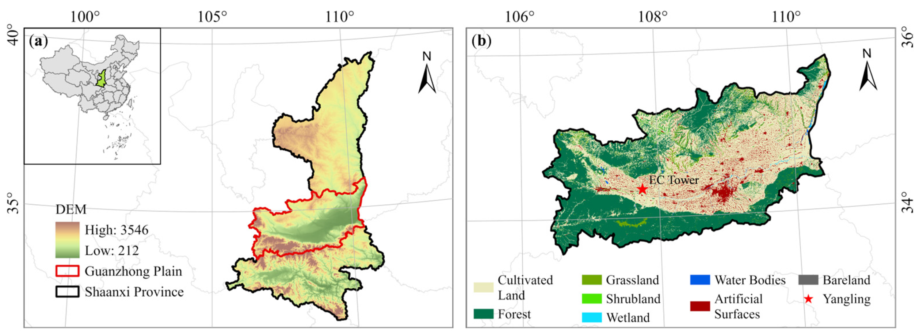
The Yangling Site (34°17′ N, 108°04′ E; 521 m a.s.l.) is located in the Guanzhong Plain of Northwest China, within the Institute of Water Saving Agriculture in Arid Areas (IWSA) at Northwest Agriculture and Forestry University (NWAFU), Shanxi Province (Figure 1) [61]. The study area experiences an average of 2000 sunshine hours and an annual mean temperature of 12.9 °C, with a frost-free period of approximately 210 days, while climatic drought events frequently occur [62]. According to the United States Department of Agriculture Soil Classification System, the soil in the study area is classified as silty clay loam [63,64], with a bulk density of 1.35 g cm−3 and a field capacity of 0.235 m3 m−3 [65,66,67].

2.2. In-Situ Data Collection and Processing

This study used an automated six-channel, tower-based SIF observation system installed approximately 2 m above the vegetation canopy to measure canopy radiance around the flux tower. The system was deployed on six tripods surrounding the flux tower to reduce potential footprint mismatch between SIF and flux observations. The instrument consisted of a cosine corrector for downwelling irradiance measurements, a spectroradiometer, and an optical multiplexer that sequentially switched between downwelling irradiance and multi-channel upwelling radiance measurements. Radiometric and spectral calibrations were performed prior to deployment to ensure measurement stability and accuracy. During data processing, dark current correction and integration time optimization were applied [68,69]. Subsequently, the “sandwich” sampling strategy (downwelling–upwelling–downwelling) was applied to further reduce the influence of rapid atmospheric variability on SIF retrieval [70]. SIF was retrieved from continuous spectral measurements using the singular value decomposition (SVD) method based on the O2-A absorption band [71,72]. The SVD method assumes that SIF-free spectra can be represented as linear combinations of singular vectors derived from a SIF-free training dataset. In this study, the training dataset consisted of continuous downwelling solar spectral measurements [73,74,75]. The prescribed fluorescence spectral shape used for retrieval was derived from SCOPE simulations [69]. Top-of-canopy (TOC) SIF in the near-infrared band was retrieved using a spectral fitting window of 740–780 nm, and the resulting values were aggregated into 30-min averages [71]. Low-quality retrievals under low illumination (photosynthetically active radiation (PAR) < 30 μmol m−2 s−1) or high solar zenith angles (>65°) were excluded [69,76].
An EC system, consisting of a three-dimensional ultrasonic anemometer, an open-circuit infrared gas analyzer, and a data logger, was mounted on an adjustable-height tripod near the spectrometry system to measure CO2 fluxes during the wheat growing season in this region. The sensor was positioned 2 m above the ground and oriented toward the prevailing wind direction. Wind speed (u) and direction, along with other boundary layer meteorological measurements, were recorded using a propeller anemometer. Air temperature (Ta) and relative humidity (RH) were recorded at 1.5 m above the soil surface using a combined temperature-humidity sensor, while Rn was measured with a four-component radiation sensor at 2 m above the soil surface. Rainfall was measured using a tipping bucket rain gauge, and G was measured with a self-regulating heat flux plate at 8 cm below the soil surface. All meteorological variables were recorded as 30-min averages using a data logger.
The 10 Hz raw data were converted into half-hour net ecosystem exchange (NEE) using EddyPro 7 software. Flux data affected by sensor malfunctions, low wind conditions (friction velocities below 0.1 m s−1), or precipitation (Pre) were excluded [65]. Missing data compensation and decomposition of CO2 into total ecosystem respiration (TER) and GPP were performed using the REddyProc online tool created by the Max Planck Institute for Biogeochemistry, with input data, including NEE, RH, Ta, soil temperature (Ts), and solar radiation (SR). The gap-filling algorithm in REddyProc efficiently fills in gaps for meteorological variables (Ta and vapor pressure deficit (VPD)) and flux data [61,77]. Thirty-minute GPP was calculated as the NEE–TER difference [56]. Based on 30-min Ta and RH data, VPD can be obtained following Campbell and Norman’s method [78].

2.3. STEMMUS-SCOPE Model

The STEMMUS-SCOPE model is a coupled model based on the soil–vegetation–atmosphere continuum. It incorporates radiative transfer, photochemical processes, and energy balance, simulating the dynamic growth of roots, SM, Ts, energy, water and carbon fluxes, and fluorescence (Figure 2) [56,79,80]. The model is primarily used to investigate vegetation responses under water-stress conditions [56,57]. Based on the initial SM profile simulated by STEMMUS, the STEMMUS-SCOPE model first calculates the water stress factor (WSF) as the limiting factor for the maximum carboxylation rate (Vcmax). Net photosynthesis (An), T, energy fluxes, GPP, and SIF were then calculated using SCOPEv1.73. The above-calculated T determines plant root water uptake (RWU) in STEMMUS. Root growth is then calculated from An. Based on RWU and dynamic root growth, STEMMUS calculates changes in Ts and SM [67,81,82]. Soil surface moisture is used to calculate the soil surface resistance, which is then used to compute Es. Overall, SM is subsequently used to calculate the WSF for the next time step. Meanwhile, SCOPE calculates the soil surface temperature using the energy balance, using it as the top boundary condition for STEMMUS. It also calculates the leaf water potential (LWP) through iteration [56]. The key functions used in STEMMUS-SCOPE are detailed in Appendix A.

2.4. STEMMUS-MLR Model

Similar to STEMMUS-SCOPE, the STEMMUS-MLR model is an SIF-driven model which couples the MLR [41] with STEMMUS (Figure 2) [60,67,79,80,81,82]. It utilizes SIF and meteorological observations to simulate the terrestrial eco-hydrological processes. First, the MLR model accurately calculates GPP using SIF through the MLR framework. Then, canopy conductivity (Gc) can be calculated based on Ball–Woodrow–Berry (BWB) canopy conductance model, using GPP and WSF, which is calculated by the initial SM from the STEMMUS simulation. Then, T can be calculated using Gc and the dual-source Penman-Monteith (PM) equations. T is passed to STEMMUS as RWU. Meanwhile, STEMMUS calculates soil surface resistance based on surface SM, which is then used to calculate Es via the PM equation. The STEMMUS model simulates the updated SM for each layer using real-time updated RWU and Es, which then serves as the starting condition for the next time step [20]. The key functions used in STEMMUS-MLR can be found in Appendix A.

2.5. Random Forest Model and SHAP Method

In this study, a Random Forest (RF) model combined with the Shapley additive explanations (SHAP) method was used to quantitatively assess the importance of SIF in simulating eco-hydrological processes. Previous studies have demonstrated that the RF model outperforms other machine learning algorithms in simulation tasks [83,84,85]. Therefore, the RF model was employed to learn and approximate the outputs of the mechanistic model, constructing a data-driven surrogate model [86,87]. Based on this, SHAP was applied to evaluate the contribution of each input variable within the surrogate model, revealing the internal response mechanisms and key driving factors of the mechanistic model [88,89]. This can enhance model interpretability and transparency and further clarify the crucial role of SIF in eco-hydrological simulations. Specifically, input variables for SHAP analysis were selected based on the forcing variables and key drivers used in the STEMMUS-SCOPE and STEMMUS-MLR frameworks. Accordingly, the explanatory features included meteorological forcing variables (e.g., Ta and u), vegetation-related variables, and SIF observations. This design ensures that the SHAP interpretation focuses on quantifying the sensitivities and relative contributions of major drivers controlling mechanistic model outputs. For surrogate modeling, RF regression was implemented in Python 3.13 using scikit-learn, with mean squared error (MSE) as the splitting criterion. Because RF includes built-in mechanisms to reduce overfitting (e.g., bootstrap aggregation and random feature selection), only the random seed (random_state = 42) was specified, and all other hyperparameters were set to the default values in scikit-learn. Subsequently, SHAP values were computed using the TreeSHAP algorithm based on the trained RF surrogate model to quantify the contribution of each driver to the model outputs and improve interpretability.

2.6. Experiment Design

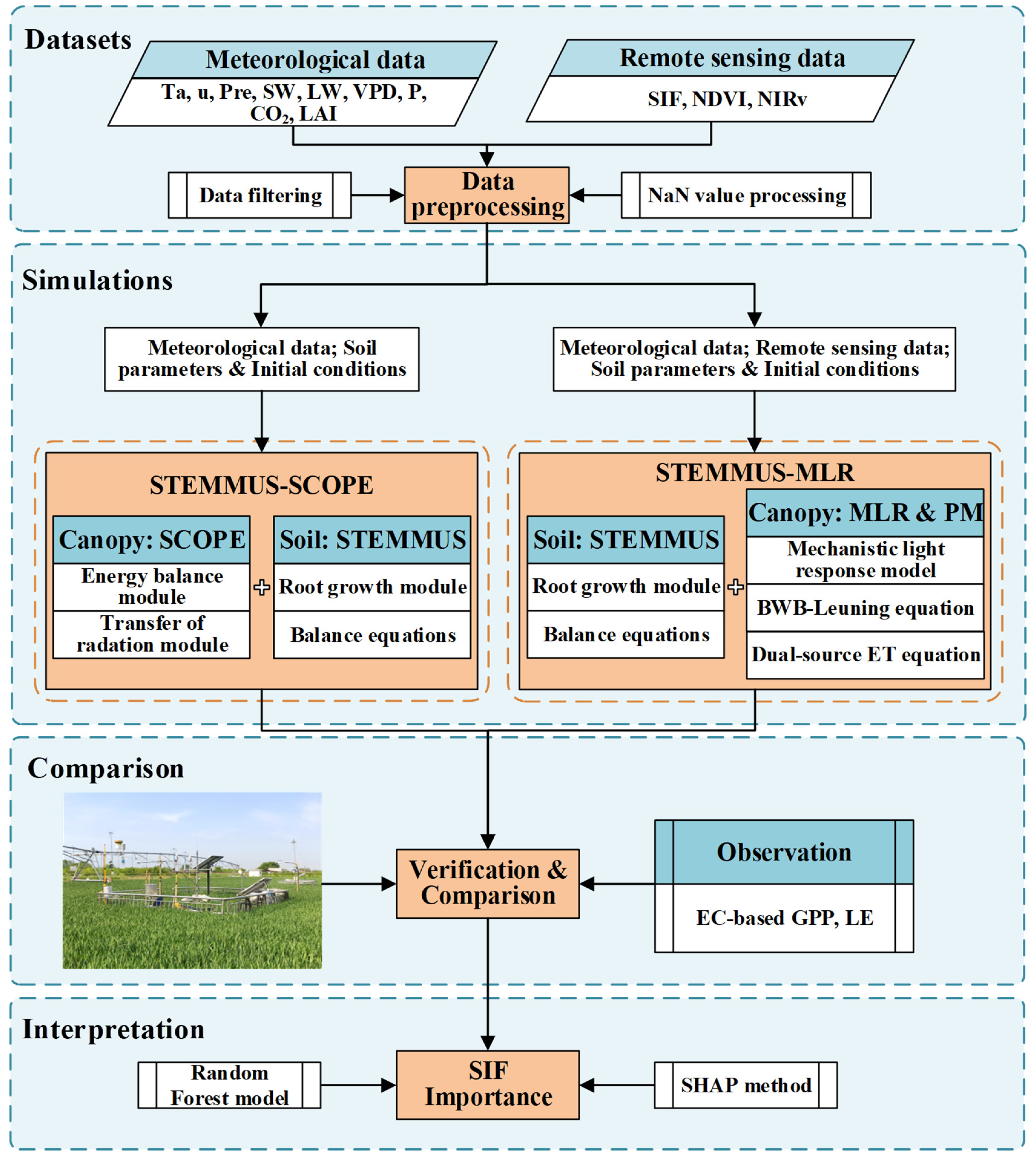
Figure 2 illustrates the workflow of this study, which consists of main components: datasets, simulations, verification, and interpretation. Datasets include meteorological observations and remote sensing data, and are used as model inputs after pre-processing, including missing value removal and variable selection. Simulations are conducted using the STEMMUS-SCOPE and STEMMUS-MLR models. The STEMMUS-SCOPE model uses meteorological data, soil parameters, and initial conditions as inputs. In contrast, the STEMMUS-MLR model simulates the ecohydrological processes by integrating remote sensing SIF with meteorological inputs. Both models use STEMMUS as the soil module, which incorporates root growth and mass balance equations. However, the two models differ in their canopy modules. The STEMMUS-SCOPE model integrates the SCOPE model, which simulates radiative transfer and energy balance processes. The STEMMUS-MLR model uses a canopy module based on the MLR framework combined with the PM equation. The simulated GPP and LE are then evaluated to systematically assess the applicability and performance of each model. Finally, the importance of SIF and meteorological inputs in eco-hydrological simulations is analyzed using the RF model combined with the SHAP analysis.

2.7. Statistical Analysis Methods

The accuracy of mechanistic models (STEMMUS-SCOPE and STEMMUS-MLR) is evaluated using the Coefficient of Determination (R2), Root Mean Square Error (RMSE) and Kling–Gupta Efficiency (KGE) [3,90,91]. The formulas for the metric are as follows:
R 2 = i = 1 n P i P ¯ O i O ¯ i = 1 n P i P ¯ 2 i = 1 n O i O ¯ 2 2
R M S E = 1 n i = 1 n P i O i 2
K G E = 1 R 1 2 + α 1 2 + β 1 2
where P i represents the i-th predicted value, P ¯ is the mean of the predicted values, O i is the i-th observed value, O ¯ is the mean of the observed values, n is the sample size, R is the Pearson correlation coefficient, α is the ratio of the standard deviations of the simulated and observed values, and β is the ratio of the mean simulated to observed values.

3. Results

3.1. In-Situ Meteorology, Fluxes, and SIF Observations

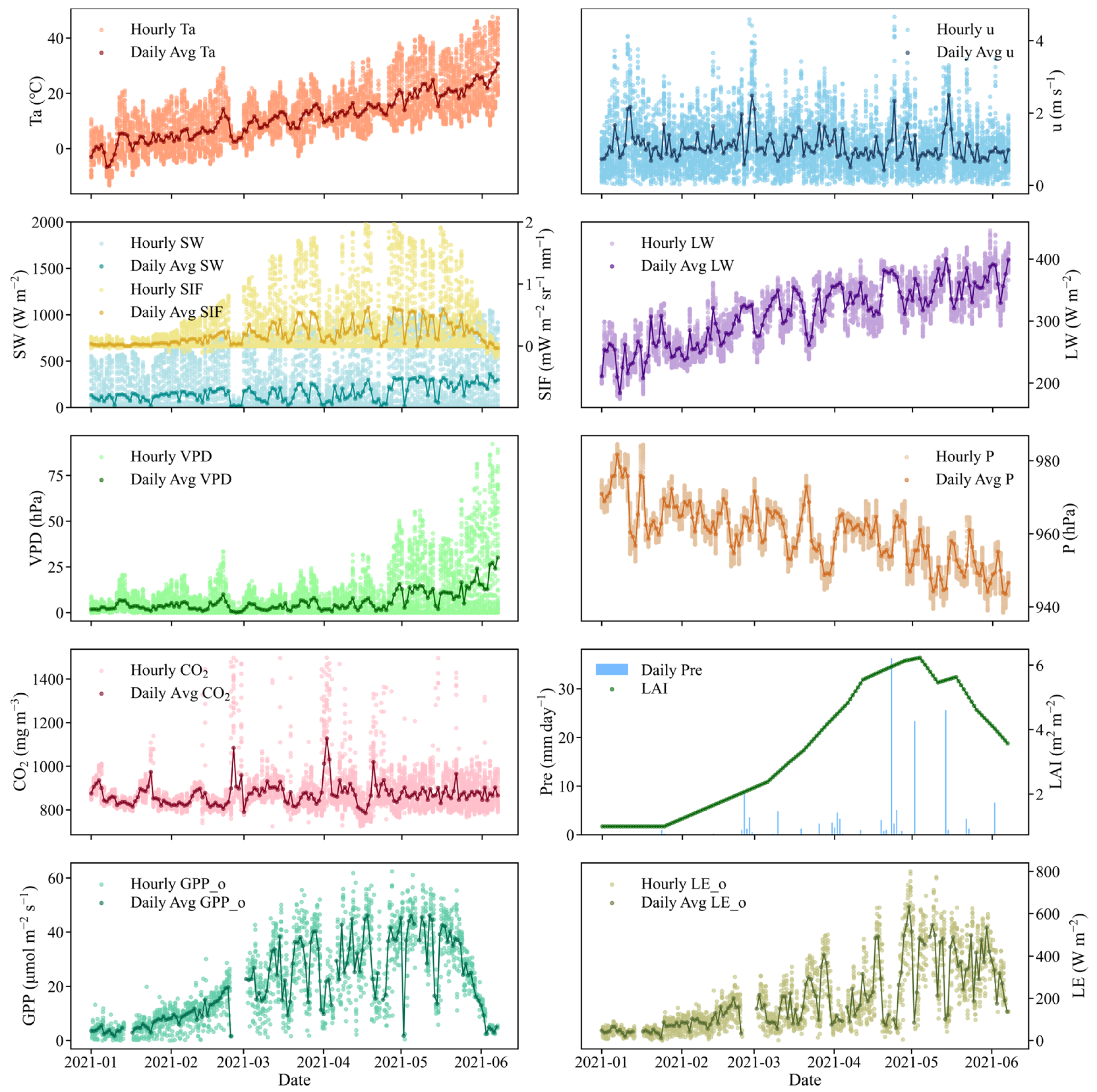
Data were collected from January to June 2021, corresponding to the winter wheat growing season. Figure 3 presents observed data aggregated at hourly and daily scales. The dataset consists of three groups: (1) meteorological variables as inputs for mechanistic models (Ta, u, Pre, shortwave radiation (SW), longwave radiation (LW), VPD, air pressure (P), leaf area index (LAI), and CO2 concentration) and (2) observed fluxes as target outputs (Rn, LE, H, GPP); and (3) remotely sensed SIF.
During the observation period, Ta ranged from −13.3 to 47.7 °C, with a mean of 11.4 °C, while P remained stable (938.4–984.6 hPa). Daily average wind was 1.09 m s−1, fluctuating between 0 and 4.66 m s−1. SW and LW showed overall increasing trends, with hourly peaks of 1068.1 W m−2 and 446.3 W m−2, respectively. Precipitation occurred mainly in May–June (totaling 149.3 mm), increasing air humidity and reducing evaporative demand. VPD decreased during Precipitation events but exhibited an overall increasing trend, with higher values in May–June than in January–April. LAI rose sharply in early February during regreening, peaked at 5.88–6.23 m2 m−2 in late April–early May, and then declined until harvest. Daily GPP peaked in April–May during vigorous wheat growth, while GPP was lower in other months due to reduced LAI and radiation. Daily mean LE peaked at ~400–450 W m−2 in early May with peak LAI.

3.2. STEMMUS-SCOPE and STEMMUS-MLR Model Simulations

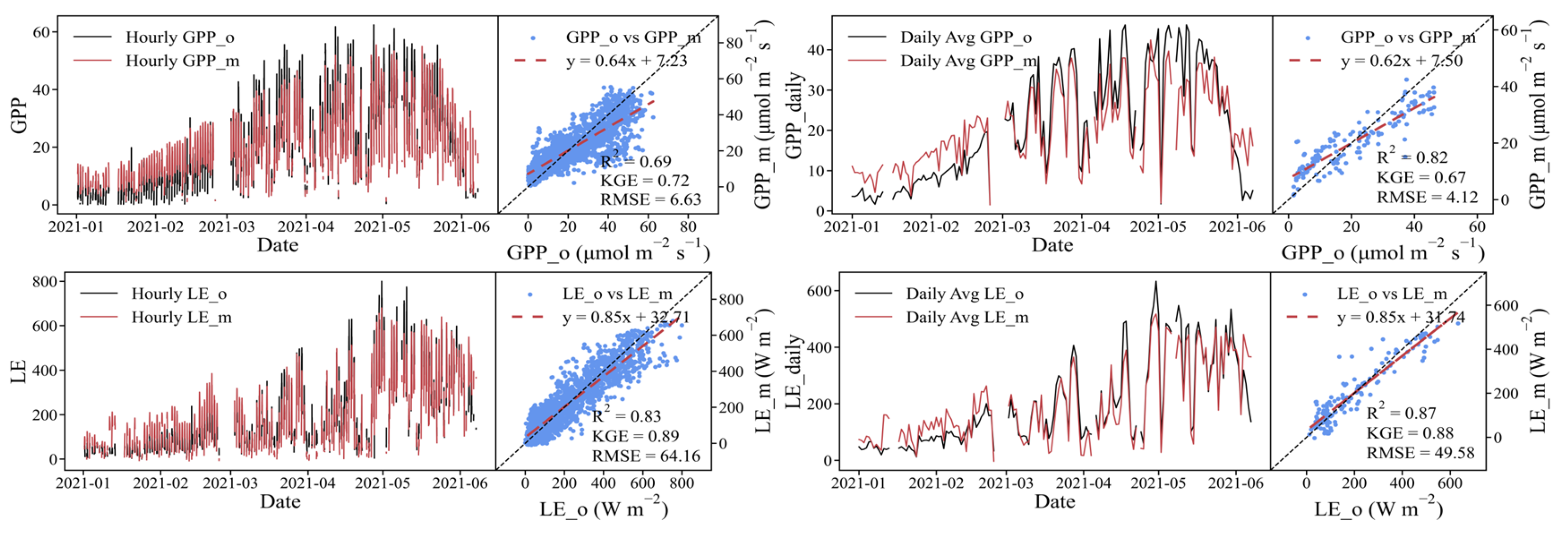
Figure 4 illustrates the simulation results of the STEMMUS-SCOPE model for both GPP and LE at hourly and daily scales. On the daily scale, the simulated trends generally match the observations, although significant deviations appear in January and June. The model performs similarly well for GPP (KGE = 0.67, slope = 0.62) and LE (KGE = 0.88, slope = 0.85), with slightly higher accuracy for LE. At the hourly scale, performance declines for GPP (KGE = 0.72, slope = 0.64) but remains robust for LE (KGE = 0.89, slope = 0.85).
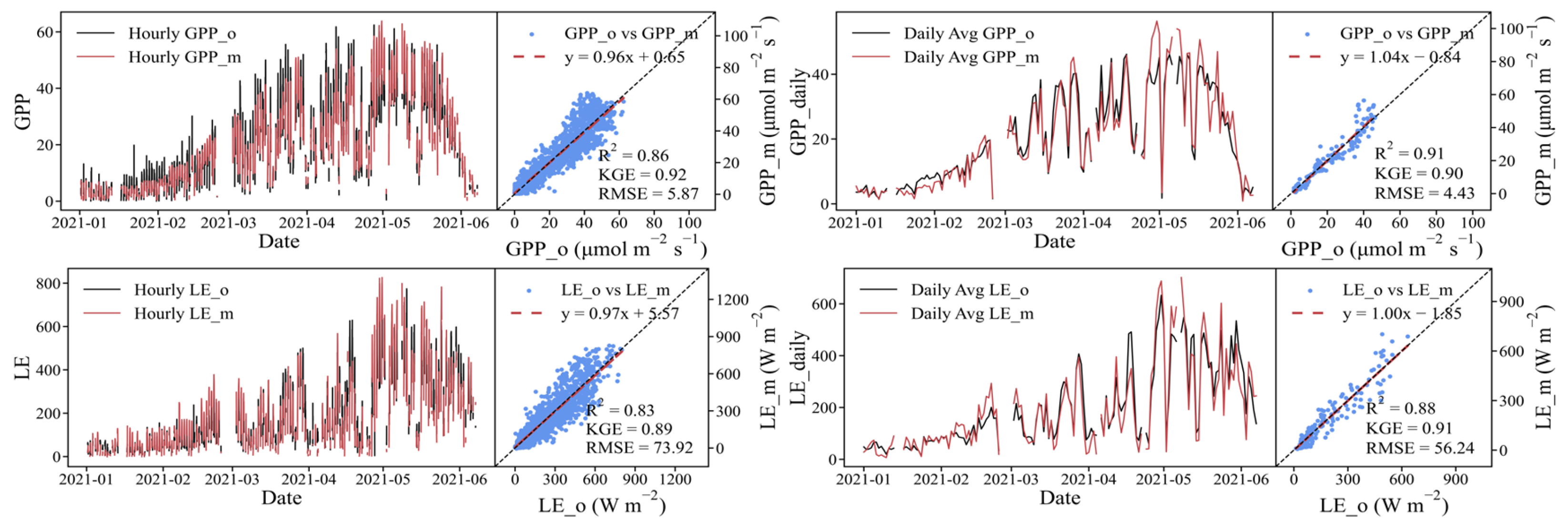
As shown in Figure 5, the STEMMUS-MLR model achieves consistently high accuracy for both fluxes. For LE, KGE reaches 0.89 at the hourly scale and 0.91 at the daily scale, with a slope of 0.97 and 1.00; while for GPP, the corresponding values are 0.92 and 0.90, with a slope of 0.96 and 1.04. Minor discrepancies occur toward the end of the study period, but simulations generally align well with observations during the main growing season, demonstrating robust overall performance.
Overall, by requiring fewer parameters, the STEMMUS-MLR model achieves improved simulations of both GPP and LE across temporal scales compared with STEMMUS-SCOPE. These findings suggest that although STEMMUS-SCOPE effectively represents eco-hydrological processes, incorporating SIF into mechanistic models can further improve simulation accuracy, both for GPP and LE.

3.3. SHAP-Based Feature Importance and Contributions of SIF and Other Factors

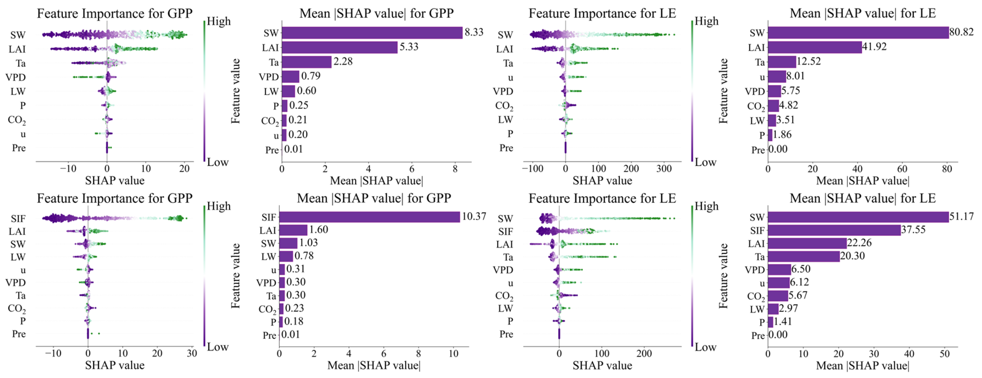
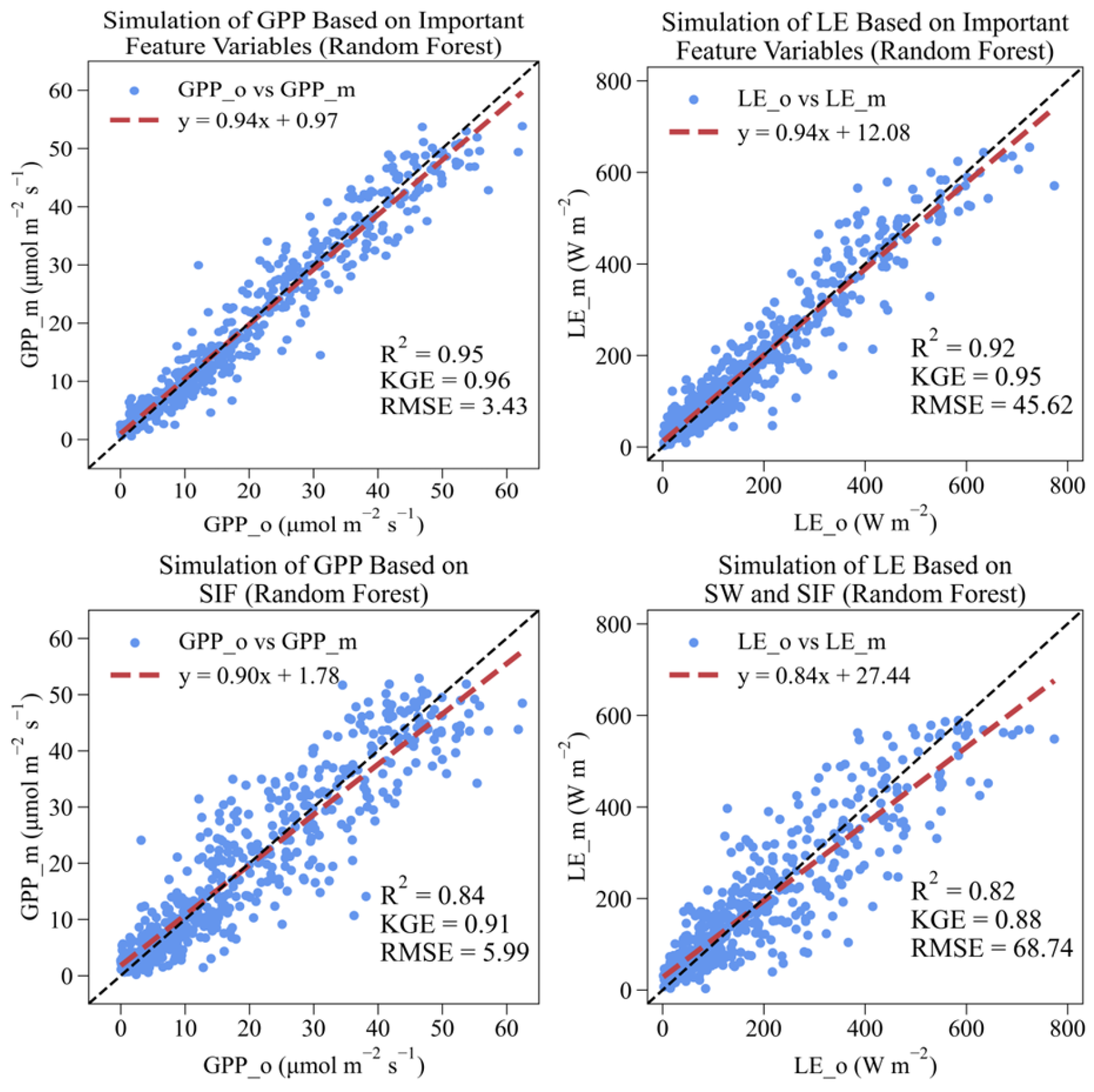
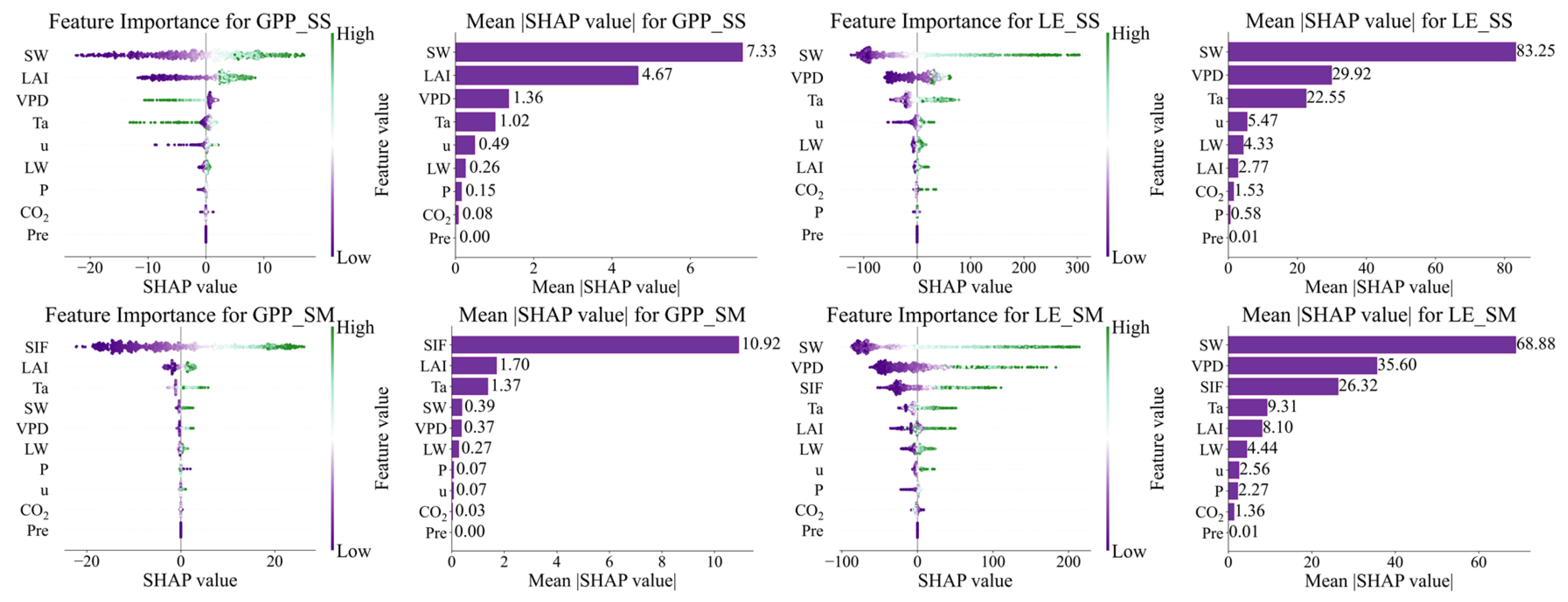
To quantify the contributions of input drivers to GPP and LE, we applied the RF model and the SHAP method for feature importance analysis. As shown in Figure 6, we compared feature importance with and without SIF to reveal the information redundancy between SIF and environmental factors. Without SIF, SW, LAI, Ta, and VPD emerged as the dominant features for GPP. However, after introducing SIF, the contributions of SW, LAI, and Ta decreased markedly, with SIF becoming the most influential predictor. This reflects the strong physiological link between SIF and GPP, as simulations using SIF alone already achieved high accuracy (KGE = 0.91, Figure 7).
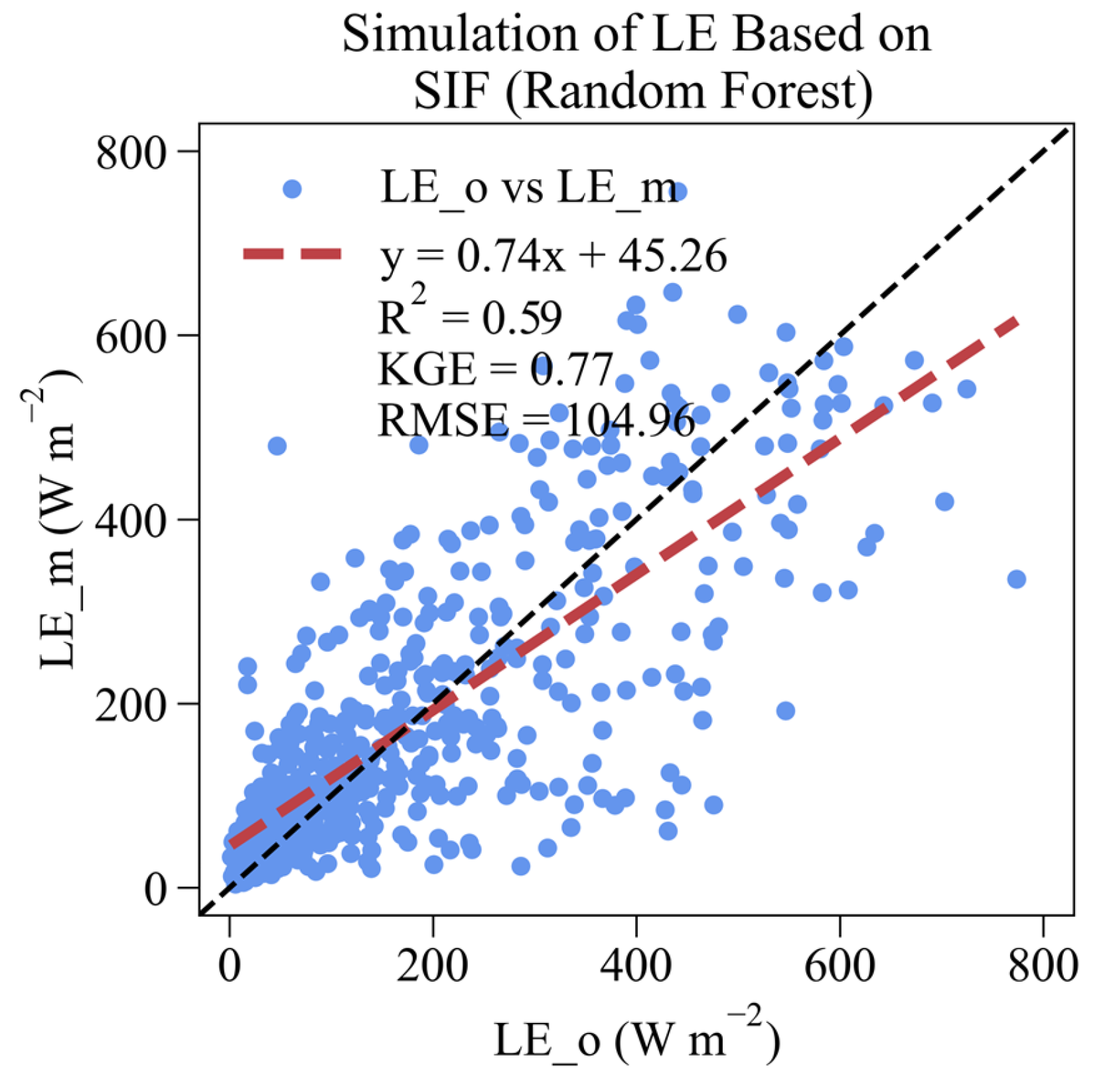
For LE, SW, LAI, and Ta were the primary predictors in the absence of SIF. After incorporating SIF, their importance declined, while SIF ranked as the second most important variable. Simulations using SW and SIF yielded high accuracy (KGE = 0.88, Figure 7), whereas SIF alone resulted in substantially lower accuracy (KGE = 0.77, Figure A1). This demonstrates that SIF alone is insufficient for LE, where radiation-driven Es remains critical. Collectively, these results indicate redundancy between SIF and variables such as SW and LAI, and suggest that SIF plays a central role in GPP modeling, while accurate LE simulations require the joint influence of radiation and soil water availability.
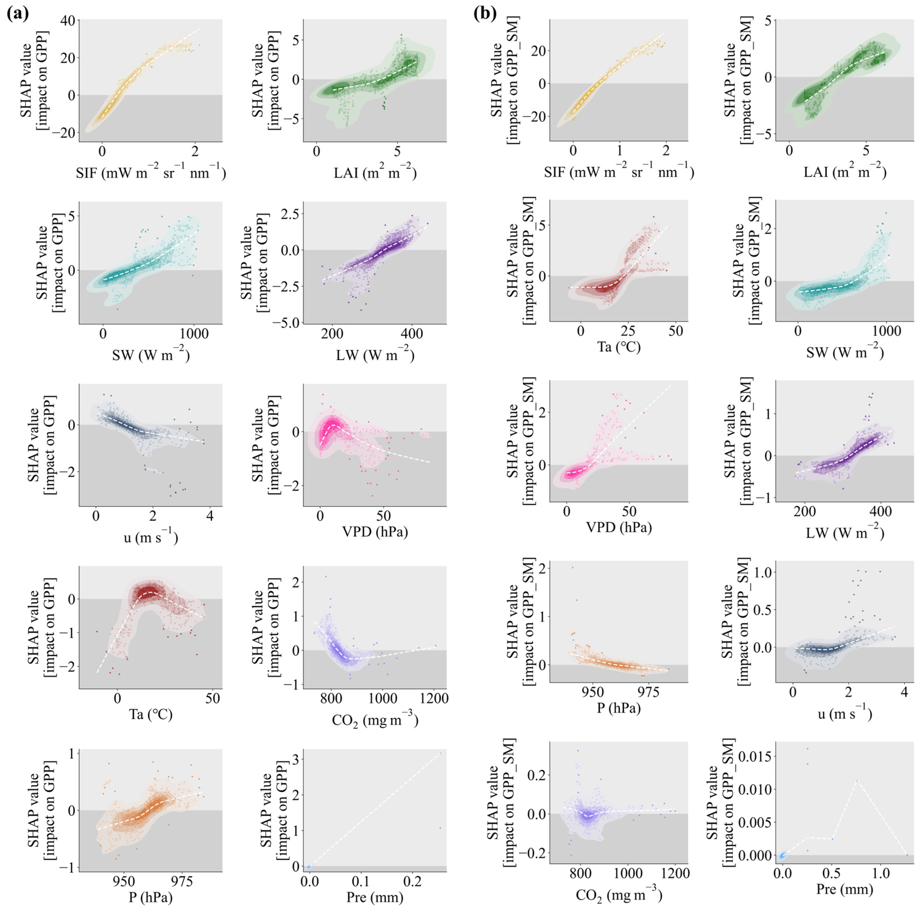
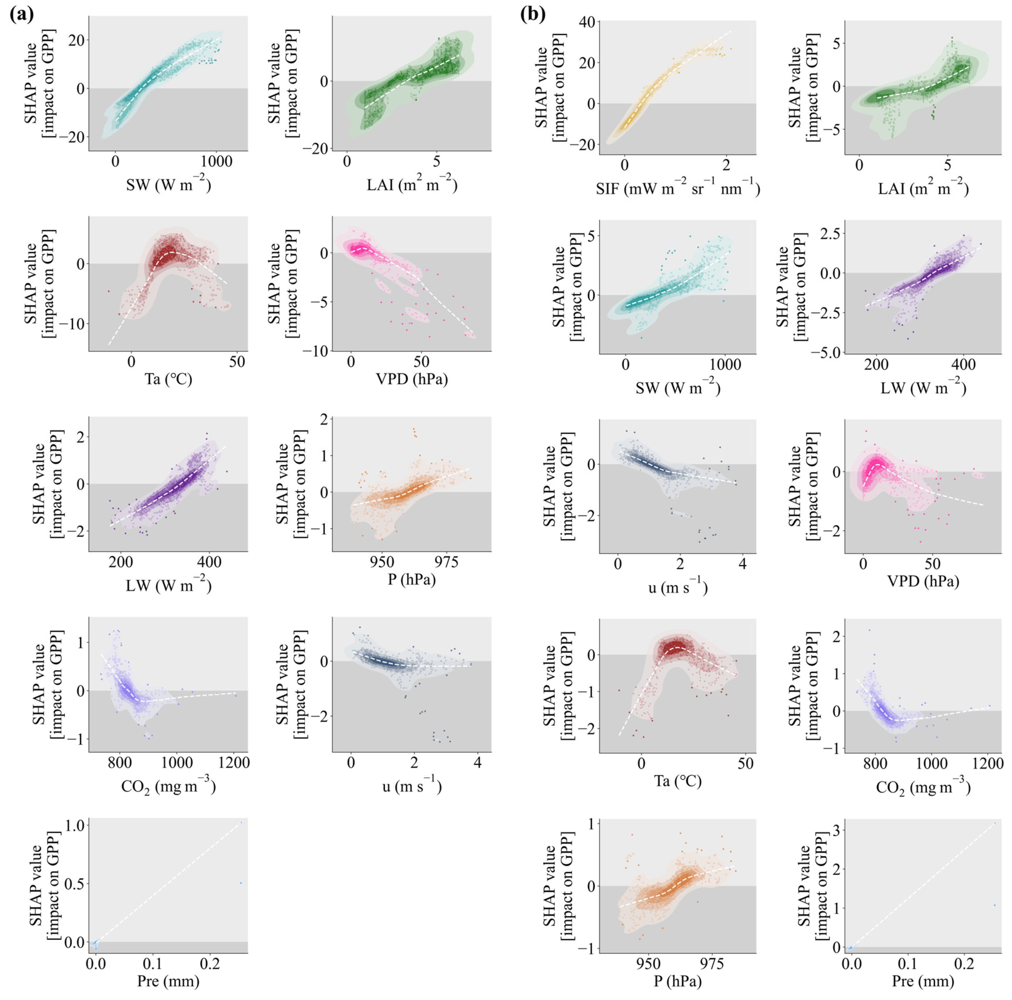
Beyond relative importance, SHAP dependence plots further revealed nonlinear relationships between drivers and fluxes (Figure 8 and Figure 9). For GPP, SIF exhibited the strongest positive association, forming a tightly clustered distribution, thereby reflecting its ability to capture dynamic changes in photosynthesis (Figure 8, right panel a). LAI showed a dual effect: negative at low values (LAI < ~4 m2 m−2) due to limited canopy light interception, but positive at higher values as canopy efficiency improved (Figure 8, right panel b). SW and LW both had generally positive contributions, highlighting the pivotal role of radiation in photosynthesis (Figure 8, right panel b).
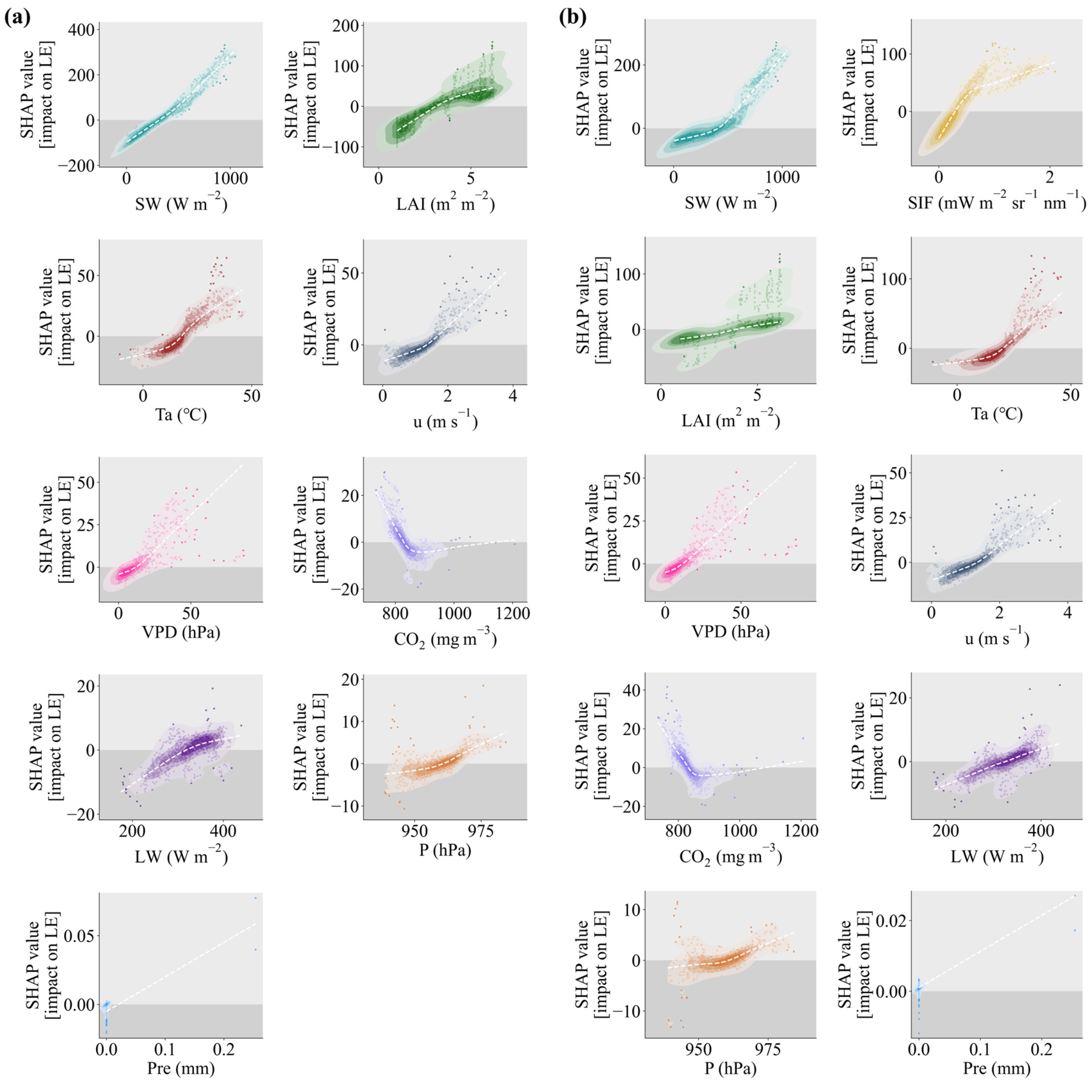
In contrast, LE simulations were primarily controlled by SW (Figure 9). Although the SHAP value of SW decreased slightly after SIF was introduced, it remained the dominant driver, confirming the importance of radiation as the main energy source for ET. Meanwhile, SIF ranked second in importance, reinforcing its complementary role but also demonstrating redundancy with other radiation- and vegetation-related variables.
Together, these results emphasize that SIF could improve the attribution and simulation of GPP and LE. Its strong explanatory power highlights its critical role in GPP estimation, while also revealing the continued importance of Es and root-soil water interactions in LE simulation.

3.4. The “Equivalent Modeling” Approach for Interpreting Mechanistic Models

To investigate how input variables shape the outputs of mechanistic models (STEMMUS-SCOPE and STEMMUS-MLR), we employed the concept of an “equivalent model”. Specifically, an RF model was trained on the simulations and forcing of the mechanistic models to approximate their behavior, and SHAP was then applied to evaluate feature importance. This approach reveals the internal response mechanisms and dominant drivers of the mechanistic models, while maintaining their physical consistency and improving interpretability.
For STEMMUS-SCOPE, the SHAP analysis highlighted SW and LAI as major drivers of GPP (Figure 10 and Figure A2), with influence patterns closely matching those from the RF model trained on observational data. This consistency indicates that STEMMUS-SCOPE captures the fundamental processes of radiation input, vegetation structure, and air humidity. However, the importance of Ta was reduced, suggesting that the model does not fully capture the regulatory effects of temperature on photosynthesis and instead overemphasizes the impact of VPD. Refining temperature-related parameterization or introducing physiologically based response functions could improve its accuracy under varying thermal conditions. For LE, STEMMUS-SCOPE overemphasized the role of VPD while underestimating the contribution of LAI. This arises from the fact that, within STEMMUS-SCOPE, VPD directly enters the LE calculation and governs stomatal conductance, thereby indirectly affecting GPP estimation (Figure 10 and Figure A3).
For STEMMUS-MLR, the contribution of SIF to GPP was generally consistent with that of the observationally trained RF model (Figure 10 and Figure A4). However, the importance of Ta increased markedly, as temperature is required for calculating the photosystem II operating efficiency (qL) within the model. In contrast, the importance of SW declined substantially. This may be attributed to the dominant role of SIF as the primary input of STEMMUS-MLR, whose feature importance far exceeded that of SW (Figure 10), thereby diminishing the latter’s influence in the model structure. These findings reveal the limitations of linear models in handling strong multicollinearity and nonlinear ecological responses. For the simulation of LE with STEMMUS-MLR, the model consistently identified SW as the dominant controlling factor (Figure 10 and Figure A5). However, the role of VPD was again overestimated, likely because the PM formulation depends strongly on VPD. At the same time, the contribution of SIF was underestimated, suggesting that the model’s capacity to fully utilize SIF data requires further improvement (Figure 10 and Figure A5). The overestimation of VPD may also stem from the fact that both the BWB canopy conductance model and the PM formulation explicitly require VPD as an input. In contrast, STEMMUS-MLR showed a weaker influence of VPD on GPP, mainly because GPP is derived directly from SIF and then used to calculate canopy conductance and T, without VPD being involved in the computation of GPP itself.

4. Discussion

4.1. SIF Better Represents GPP than LE

SIF has been widely recognized as a reliable remote sensing proxy for photosynthetic activity [44,50,92]. Physiologically, SIF is emitted as a by-product of photosynthesis, representing a small fraction of APAR. It is closely linked to photosystem II activity, reflecting light-use efficiency and electron transport rates in leaves [44,50,93]. Because of this mechanistic link, numerous studies have consistently demonstrated a strong correlation between SIF and GPP across ecosystems and climate regimes [50,52,53]. Our findings further confirm that SIF plays a more dominant role in simulating GPP compared to traditional meteorological variables, providing a direct, observation-based constraint on photosynthetic dynamics that climate-driven mechanistic models often struggle to reproduce.
In contrast, the role of SIF in representing LE or ET is far less robust. Unlike GPP, which is directly tied to photochemistry, LE is influenced by multiple physiological and hydrological processes, including stomatal conductance, VPD, SM availability, and aerodynamic conditions [94,95,96,97]. SIF primarily reflects the physiological status of leaves and their photosynthetic activity but does not account for non-photosynthetic components of water fluxes, such as Es and canopy interception [51,98]. This limitation is particularly evident in water-limited or semi-arid ecosystems, where Es can contribute substantially to total LE [99,100].
Moreover, under drought stress, stomatal closure can strongly reduce transpiration without necessarily inhibiting the photochemical activity that generates SIF, leading to a decoupling of the SIF–LE relationship [101,102]. These physiological mechanisms explain why empirical or machine learning models relying solely on SIF often produce biased ET estimates, particularly under water stress or heterogeneous soil conditions. This highlights the importance of coupling SIF observations with process-based models to better represent both photosynthetic and non-photosynthetic components of water fluxes, rather than relying on SIF alone for ET or LE estimation.

4.2. The Role of SIF in Mechanistic Models

Mechanistic models are extensively employed to simulate eco-hydrological processes based on fundamental principles, such as mass and energy conservation [103,104]. These models rely on detailed physical parameters [105,106]. Their explicit parameterization of complex processes and adherence to energy and mass conservation generally yield more reliable simulations when driven by regional datasets [107,108]. Mechanistically integrating SIF with environmental variables, such as SM, VPD, and canopy conductance, has been shown to improve ET estimation [97,109]. In this study, the climate-driven mechanistic model (STEMMUS-SCOPE) exhibited lower accuracy compared with the SIF-driven model (STEMMUS-MLR). This finding further proves that relying solely on meteorological variables and LAI cannot fully represent the underlying physiological processes of vegetation. In contrast, STEMMUS-MLR, which integrates SIF as the primary input, outperformed STEMMUS-SCOPE in simulating both GPP and LE.
Structurally, STEMMUS-SCOPE and STEMMUS-MLR share the same STEMMUS soil module but differ mainly in their canopy and photosynthesis representations. Specifically, STEMMUS-SCOPE uses a multilayer radiative transfer and energy balance scheme to simulate canopy radiation transfer, vertical profiles of temperature and humidity, and layer-specific photosynthesis and transpiration [56]. In contrast, STEMMUS-MLR, a big-leaf model, uses a simplified MLR framework and dual-source PM model. It lacks the complex multilayer canopy structure and requires far fewer physiological parameters [20,60]. Consequently, STEMMUS-MLR significantly reduces computational cost compared with STEMMUS-SCOPE, with a runtime approximately one-tenth as long [20]. Although structurally simpler, the photosynthesis formulation of STEMMUS-MLR remains consistent with the Farquhar–von Caemmerer–Berry (FvCB) biochemical model implemented in SCOPE. The key difference is in how the electron transport rate is estimated. In STEMMUS-SCOPE, within the FvCB model, the maximum electron transport rate is mainly driven by PAR via radiative transfer simulations. In STEMMUS-MLR, the actual electron transport rate is constrained by SIF observations. Although a relatively simple structure in STEMMUS-MLR, this study highlights that SIF effectively represents photosynthetic processes, compensating for the limitations of climate-driven models that rely on precise parameterization of photosynthetic capacity (e.g., Vcmax) and stomatal regulation, thereby improving overall model performance.
From a modeling perspective, two key implications can be drawn: First, integrating SIF into ecohydrological models provides a powerful constraint on photosynthesis-related processes, significantly improving GPP simulations. Second, accurate representation of LE requires explicit consideration of additional hydrometeorological variables (e.g., SM, VPD, and aerodynamic resistance) and process-based representations of Es. Therefore, while SIF-driven models hold promise for advancing carbon cycle modeling, their application to water fluxes must be complemented by other data sources to avoid systematic biases. In summary, this study reinforces the role of SIF as a robust indicator of photosynthetic carbon uptake while cautioning against its direct application to LE or ET modeling.

4.3. Limitations and Future Perspectives

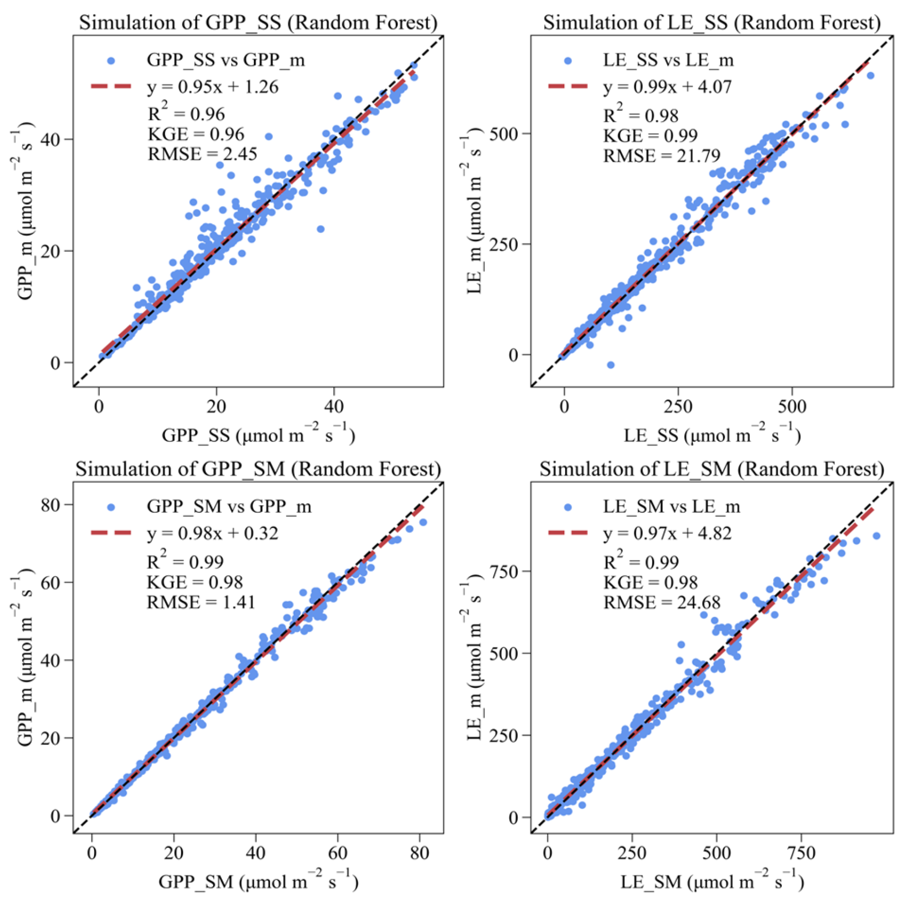
This study also has several limitations: First, the SHAP analysis was performed using an RF surrogate model rather than being applied directly to the mechanistic models. Although the surrogate model accurately reproduces the outputs of STEMMUS-MLR (e.g., GPP: KGE = 0.98; LE: KGE = 0.98) and STEMMUS-SCOPE (e.g., GPP: KGE = 0.96; LE: KGE = 0.99; Figure A6), SHAP explanations primarily reflect statistical relationships learned by the RF model rather than strictly mechanistic processes. However, because the surrogate model inputs were selected from the same forcing variables used in the mechanistic models, the high agreement between surrogate predictions and mechanistic outputs suggests that the machine learning model can reliably capture the underlying relationships embedded within the mechanistic frameworks. Second, the study focuses solely on the Yangling Site and C3 cropland, which limits the generalizability of the results across different agroecosystems, climatic conditions, or crop types. Third, although the study area is prone to climatic droughts, the dataset only covers hourly observations from January to June 2021. The relatively short time span may not allow for a fully comprehensive assessment of drought impacts on ecosystem functioning, which could influence the robustness of the results. Future research should expand to multiple sites and climatic zones to improve representativeness and to better evaluate the influence of extreme events, such as droughts, on model performance.
In the future, integrating machine learning, mechanistic models, and remote sensing signals offers promising opportunities. While machine learning approaches provide high computational efficiency, particularly at regional scales, mechanistic models offer greater robustness in evaluating ecosystem responses to extreme climate events and could serve as valuable training data for machine learning models. In addition, SIF provides direct physiological information of vegetation and mitigates the influence of parameter uncertainties on model simulations. Future work will utilize multi-year, multi-site datasets, including TROPOMI SIF satellite products and FLUXNET long-term flux observations, to evaluate ecosystem functioning across broader spatial and temporal scales. In addition, C3 and C4 vegetation types in specific vegetation types (e.g., cropland and grassland) will be identified and classified to support more robust and accurate cross-ecosystem and cross-climate assessments. By leveraging the complementary strengths of these approaches, future studies can achieve more accurate simulations of ecosystem functioning across broader spatial and temporal scales using SIF, thereby advancing predictions of ecosystem responses to climatic stressors. Moreover, these enhanced simulations can inform practical applications, including optimizing irrigation schedules, guiding water resource management, and supporting carbon accounting at farm or regional scales.

5. Conclusions

This study evaluated the performance of two eco-hydrological models in simulating LE and GPP under different levels of data availability. Results show that incorporating SIF substantially improved the accuracy of both hourly and daily simulations in STEMMUS-MLR (GPP: KGE = 0.90; LE: KGE = 0.91), outperforming STEMMUS-SCOPE (GPP: KGE = 0.67; LE: KGE = 0.88), which relied solely on climatic inputs. This indicates that SIF serves as a key driver that enhances the predictive capability of process-based eco-hydrological models. In STEMMUS-MLR, SIF directly improves GPP estimation and, consequently, strengthens the simulation of T and SM dynamics, leading to a more realistic representation of eco-hydrological processes. The SHAP analysis further reveals that the improved accuracy stems from the integration of physiological information carried by SIF—capturing vegetation responses to radiation, Ta, and structural information from LAI. However, the representation of certain driving processes in the model still has room for improvement. Overall, these findings highlight the critical role of SIF in advancing eco-hydrological modeling of semi-arid cropland ecosystems and its potential application in Earth System Models. Practically, SIF-based models can support water management decisions, guide irrigation planning, and improve carbon accounting, thereby bridging the gap between mechanistic modeling and real-world ecosystem management. Building on this, future research should explore the development of digital twin systems by incorporating advanced remote sensing signals into mechanistic models.

Author Contributions

Conceptualization, Y.W.; methodology, Y.W. and J.Y.; software, Y.W.; validation, A.C. and Y.W.; formal analysis, A.C. and Y.W.; investigation, Y.W.; resources, Q.Y. and H.C.; data curation, Y.W. and X.P.; writing—original draft preparation, A.C. and Y.W.; writing—review and editing, Y.W., Q.Z., X.M., L.L., X.L., Z.L., Y.Z. and Z.S.; visualization, A.C. and Y.W.; supervision, Y.W.; project administration, Y.W.; funding acquisition, Y.W. All authors have read and agreed to the published version of the manuscript.

Funding

This research was funded by the National Natural Science Foundation of China, grant number 42105119, 52179046, 42071328, and 41901293.

Data Availability Statement

Data and code used in this study will be available on request.

Acknowledgments

We thank the editor and anonymous reviewers for their valuable comments, which helped us improve the manuscript.

Conflicts of Interest

The authors declare no conflicts of interest.

Abbreviations

The following abbreviations are used in this manuscript:
AnNet Photosynthesis
APARAbsorbed Photosynthetically Active Radiation
BWBBall–Woodrow–Berry Canopy Conductance Model
ECEddy Covariance
EsSoil Evaporation
ETEvapotranspiration
EVIEnhanced Vegetation Index
FvCBFarquhar–von Caemmerer–Berry
GSoil Heat Flux
GcCanopy Conductivity
GPPGross Primary Productivity
HSensible Heat Flux
IWSAThe Institute of Water Saving Agriculture in Arid Areas
JElectron Transport Rate
KGEKling–Gupta Efficiency
LELatent Heat Flux
LWLongwave Radiation
LAILeaf Area Index
LWPLeaf Water Potential
MLRMechanistic Light Response Model
MSEMean Squared Error
NEENet Ecosystem Exchange
NPQNon-Photochemical Quenching
NDVINormalized Difference Vegetation Index
NWAFUNorthwest Agriculture and Forestry University
PAir Pressure
PMDual-source Penman-Monteith Equations
PARPhotosynthetically Active Radiation
PrePrecipitation
qLPhotosystem II Operating Efficiency
R2Coefficient of Determination
RFRandom Forest
RHRelative Humidity
RnNet Radiation
RWURoot Water Uptake
RMSERoot Mean Square Error
SMSoil Moisture
SRSolar Radiation
SWShortwave Radiation
SIFSolar-induced Chlorophyll Fluorescence
SVDSingular Value Decomposition
SHAPShapley Additive Explanations
SPACSoil-plant-atmosphere Continuum
SCOPESoil Canopy Observation, Photochemistry, and Energy Fluxes Model
STEMMUSSimultaneous Transfer of Energy, Mass, and Momentum in Unsaturated Soil
TTranspiration
TaAir Temperature
TsSoil Temperature
TERTotal Ecosystem Respiration
TOCTop-of-canopy
uWind Speed
VPDVapor Pressure Deficit
VcmaxMaximum Carboxylation Rate
WSFWater Stress Factor

Appendix A

Appendix A.1. STEMMUS-SCOPE

Photosynthesis and Evapotranspiration Under Water Stress in SCOPE

In the SCOPE model, C4 photosynthesis is computed as the minimum of three limiting carboxylation rates [110,111]: (1) the Rubisco (enzyme)-limited rate (Vc; Equation (A1)); (2) the RuBP regeneration (electron transport/light)-limited rate (Ve; Equation (A2)); and (3) under low CO2 conditions, the rate limited by intercellular CO2 partial pressure (pi; Vs; Equation (A3)):
V c = V c m a x W S F
V e = J 6
V s = p i ( k p L p i ) / P
A n = m i n V c , V e , V s .
In the SCOPE model, C3 photosynthesis is computed as the minimum of two limiting carboxylation rates [112]: (1) the Rubisco (enzyme)-limited rate (Vc; Equation (A5)) and (2) the RuBP regeneration (electron transport/light)-limited rate (Ve; Equation (A6)):
V c = V c m a x W S F C i Γ * C i + K c ( 1 + O i K o )
V e = J ( C i Γ * ) 4 ( C i + 2 Γ * )
A n = m i n V c , V e
C i = C a ( 1 1 m R H )
where V c m a x represents the maximum carboxylation rate (μmol m−2 s−1); p i represents the intercellular CO2 partial pressure (Pa); k p is the pseudo-first-order rate constant of PEP carboxylase with respect to C i ; and P denotes atmospheric pressure. An is the net photosynthesis rate (μmol m−2 s−1); WSF denotes the total water stress factor; J is the electron transport rate (μmol m−2 s−1); Ci is the intercellular CO2 concentration (μmol m−3); Ca is the CO2 concentration in the boundary layer (μmol m−3); and m is the Ball–Berry parameter; and RH is the relative humidity at the leaf surface (%).
In addition, the leaf stomatal resistance, rc (s m−1), is calculated as follows:
r c = 0.625 ( C s C i ) A n ρ a M a 10 12 p
where ρ a is the air density (kg m−3), M a is the molecular mass of dry air (g mol−1), and p is the atmospheric pressure (hPa).
Latent heat flux (LE) is calculated as follows:
L E = λ ( q i q a ) r a + r c
where λ is the latent heat of vaporization of water (J kg−1), q i is the humidity within stomata or soil pores (kg m−3), q a is the humidity above the canopy (kg m−3), r c is the stomatal or soil surface resistance (s m−1), and r a is the aerodynamic resistance (s m−1).
In Bayat et al. [113], the water stress factor was calculated solely from root-zone soil moisture, without accounting for root length distribution. In this study, the water stress factor incorporates both root length distribution and root-zone water content. We adopted a sigmoid formulation instead of the piecewise function proposed by Bayat et al. [113]. The calculations are given as follows:
W S F = i = 1 n R F i W S F ( i )
W S F ( i ) = 1 1 + e 100 θ s a t S M ( i ) θ f + θ w 2
where θ w is the soil water content at the wilting point, θ f is the soil water content at field capacity, and θ s a t is the saturated soil water content. WSF(i) denotes the water stress factor in soil layer i; RF(i) represents the fraction of root length in soil layer i (see Appendix A.4); and SM(i) is the soil moisture content in soil layer i.

Appendix A.2. Governing Equations in STEMMUS

Appendix A.2.1. Soil Water Conservation Equation

t ρ L θ L + ρ V θ V = z q L h + q L T + q L a + q V h + q V T + q V a S = ρ L z K h z + 1 + D T D T s z + K γ w P g z + z D V h h z + D V T T s z + D V a P g z S
where ρ L and ρ V (kg m−3) denote the densities of liquid water and water vapor, respectively; qL and qV (m3 m−3) represent the corresponding volumetric contents; z (m) is the vertical coordinate (positive upward); S (cm s−1) is the sink term describing root water extraction; K (m s−1) is the hydraulic conductivity; h (cm) is the pressure head; Ts (°C) is the soil temperature; Pg (Pa) is the pore-air pressure; and γ w (kg m−2 s−2) is the specific weight of water. DTD (kg m−1 s−1 °C−1) is the transport coefficient for adsorbed liquid flow induced by a temperature gradient, DVh (kg m−2 s−1) is the isothermal vapor conductivity, DVT (kg m−1 s−1 °C−1) is the thermal vapor diffusion coefficient, and DVa is the advective vapor transfer coefficient [79,80]. q L h , q L T , and q L a (kg m−2 s−1) are the liquid water fluxes driven by gradients of matric potential, temperature, and air pressure, respectively, whereas q V h , q V T , and q V a (kg m−2 s−1) are the corresponding water vapor fluxes.

Appendix A.2.2. Dry Air Conservation Equation

t ε ρ d a S a + H c S L = z D e ρ d a z + ρ d a S a K g μ a P g z H c ρ d a q L ρ L + θ a D V g ρ d a z
where ε denotes the soil porosity; ρ d a (kg m−3) represents the density of dry air; Sa (=1 − SL) defines the soil air saturation; SL (=θL/ ε ) indicates the soil saturation; Hc is Henry’s constant; De (m2 s−1) corresponds to the molecular diffusivity of water vapor in soil; Kg (m2) is the intrinsic air permeability; ma (kg m−2 s−1) denotes the air viscosity; qL (kg m−2 s−1) represents the liquid water flux; θ a(= θ V) indicates the volumetric fraction of dry air in soil; and DVg (m2 s−1) is the gas-phase longitudinal dispersion coefficient [79,80].

Appendix A.2.3. Energy Balance Equation

t ρ s θ s C s + ρ L θ L C L + ρ V θ V C V + ρ d a θ a C a T s T r + ρ V θ V L 0 ρ L W θ L t = z λ e f f T z z [ q L C L T s T r + q V ( L 0 + C V T s T r ) + q a C a T s T r ] C L S T s T r
where Cs, CL, CV, and Ca (J kg−1 °C−1) denote the specific heat capacities of solids, liquid water, water vapor, and dry air, respectively. The densities of solids ( ρ s ), liquid water ( ρ L ), water vapor ( ρ V ), and dry air ( ρ d a ) are expressed in kg m−3. θ s represents the volumetric fraction of solids in soil, while θ L , θ V , and θ a correspond to the volumetric fractions of liquid water, water vapor, and dry air. Tr (°C) is the reference temperature, and L0 (J kg−1) is the latent heat of vaporization of water at Tr. W (J kg−1) denotes the differential heat of wetting, which is released when a small amount of free water is added to the soil matrix. The effective thermal conductivity of soil is λ e f f (W m−1 °C−1), and qL, qV, and qa (kg m−2 s−1) represent the fluxes of liquid water, water vapor, and dry air, respectively.

Appendix A.3. Dynamic Root Growth Modeling

Appendix A.3.1. Root Front Growth

The initial root front depth is set based on the sowing depth for directly sown crops or assigned an initial value for transplanted or perennial crops. Root front growth ceases upon reaching a specific soil depth, encountering a physical or chemical barrier, or attaining the phenological stopping stage:
Z = 0 T a i r < T m i n T a i r T m i n R G R T m i n < T a i r < T m a x T m a x T m i n R G R T m a x < T a i r
D Z t = D Z t 1 + Z
where Z denotes the root front growth at the t-th time step; D Z (cm) represents the root zone depth; T a i r (°C) is the air temperature; and Tmin (°C) and Tmax (°C) are the minimum and maximum temperatures for root growth, respectively. RGR (cm °C−1 day−1) indicates the root front growth rate.

Appendix A.3.2. Root Length Growth

In this study, root distribution within the root zone was determined by simulating root length increment across individual soil layers:
R l _ t o t = A n f r r o o t R C R D π r r o o t 2 .
The fraction of net assimilation allocated to roots ( f r r o o t ) is modeled as a function of leaf area index (LAI) and soil water content in the root zone. A n denotes the net assimilation rate (μmol m−2 s−1). R C represents the carbon-to-dry-matter ratio in roots, R D is the root density (g m−3), r r o o t denotes the root radius, and R l _ t o t (m m−3) indicates the total root length increment.
Limiting factors for carbon allocation were preliminarily calculated, incorporating root zone soil moisture availability ( A W ) and light availability ( A L ):
A W = m a x 0.1 , m i n 1 , W S F
A L = m a x 0.1 , e K e L A I
f r r o o t = m a x r m i n , r 0 3 A L A L + 2 A W
where W S F denotes the mean soil moisture stress factor within the root zone, and the light extinction coefficient is constant ( K e = 0.15 ).
The minimum allocation coefficient to fine roots is r m i n ( = 0.15 ), while r 0 represents the coefficient for theoretically unstressed fine root allocation:
R l ( i ) = R l _ t o t R F ( i )
where R F ( i ) denotes the fraction of root growth allocated to layer i, and R l ( i ) represents the root length increment in that layer.
For soil layers i = 1 to n − 1, where i = 1 corresponds to the top soil layer:
R l i t = R l i t 1 + R l i .
For the bottom soil layer, i = n:
R l i t = R l i t 1 + R l i + R l f r o n t
where R l i t and R l i t 1 denote the root lengths of layer i at time steps t and t − 1, respectively, and
R F ( i ) = R l ( i ) R l T
where R l T represents the total root length within the root zone, while R l ( i ) indicates the root length in soil layer i.
At the root front, density is specified and estimated using the parameter L v _ f r o n t , with root length growth directly governed by the root front growth rate Z :
R l f r o n t = L v _ f r o n t Z .

Appendix A.4. Root Water Uptake

Root water uptake and transpiration were calculated using the following equation:
i = 1 n ψ s , i ψ l r s , i + r r , i + r x , i = 0.622 P ρ d a ρ V e l e a r c + r a = T
where ψs,i represents the soil water potential of layer i (pressure head, m) and follows the soil moisture function formulated by Van Genuchten [114]; ψl denotes the leaf water potential (m); rs,i is the soil hydraulic resistance (s m−1); rr,i corresponds to the radial root resistance (s m−1); and rx,i is the plant axial resistance from soil to leaves (s m−1). el and ea denote the vapor pressures of the leaf and atmosphere (hPa), respectively, while ra and rc represent the aerodynamic and canopy resistances (s m−1), respectively. ρ d a represents the density of dry air (kg m−3), ρ V denotes the density of water vapor, P indicates atmospheric pressure (Pa), and 0.622 corresponds to the molar mass ratio of water to air.
Soil hydraulic resistance, r s , was calculated according to Reid and Huck [115] as:
r s = 1 B · K · L v · Δ d
where B denotes the root length activity factor, K is the soil hydraulic conductivity (m s−1), L v represents root length density (m m−3), and Δ d indicates the thickness of the soil layer (m). The root length activity factor, B, was computed as:
B = 2 π l n π R D 1 / 2 / r r o o t
where r r o o t denotes the root radius (m).
The radial root resistance, r r , was estimated following Reid and Huck [115]:
r r = P r θ s a t / θ L v Δ d
where P r denotes the root radial resistivity (s m−1).
Xylem resistance, r x , was calculated according to Klepper et al. [116]:
r x = P a Z m i d 0.5 f L v
where P a represents root axial resistivity (s m−3), Z m i d denotes the midpoint depth of the soil layer, and f is the fraction of roots at a given depth that connect directly to the stem base relative to the total roots crossing a horizontal plane at that depth. Based on Klepper et al. [116], f can be approximated as 0.22.
The updated root water uptake term is expressed as:
S i = ψ s , i ψ l r s , i + r r , i + r x , i .
Unlike previous studies that compute compensatory water uptake and hydraulic redistribution after evaluating standard water uptake for each soil layer, this study calculates the sink term using a physically based model that incorporates both root and soil hydraulic resistances rather than merely the root fraction. Consequently, the effects of compensatory water uptake and hydraulic redistribution are inherently accounted for in the sink term calculation.

Appendix A.5. STEMMUS-MLR

Appendix A.5.1. MLR Model

The original MLR model offers a level of rigor comparable to the FvCB model while requiring fewer parameters to mechanistically estimate GPP from SIF (for C3 species, [41]):
G P P = C c Γ * 4 C c + 8 Γ * × q L × Φ P S I I m a x × ( 1 + k D F ) ( 1 Φ P S I I m a x ) × f e s c × S I F
where Cc denotes the CO2 partial pressure within the chloroplast (μbar), Γ* represents the CO2 partial pressure at the chloroplastic compensation point (μbar), qL indicates the fraction of open PSII reaction centers, and SIF is the broadband total SIF emitted by PSII at the canopy top (μmol m−2 s−1). The maximum photochemical quantum yield of PSII (ΦPSIImax), assumed stable under non-stress conditions, was set to 0.86 for optimally managed winter wheat in this study [117]. The ratio of KD (rate constant for constitutive heat loss) to KF (rate constant for fluorescence emission), denoted as KDF, was assumed to be nine [61], while fesc corresponds to the SIF escape probability.

Appendix A.5.2. Calculation of qL Proposed by Liu, et al. [69]

Liu, et al. [69] introduced a SIF-informed qL method (hereafter called MLR-SIF model), which accurately estimates GPP for winter wheat, in addition to the PAR-based qL method. By incorporating SIF, this method accounts for various environmental, physiological, and structural factors influencing qL, eliminating the necessity to explicitly estimate qL across various canopy layers:
q L = m δ × S I F T O T _ F U L L _ P S I I 1 / m + m
m = m o p t × H d × e x p ( H a × ( T L e a f T o p t ) T L e a f × R × T o p t ) ) H d H a × ( 1 e x p ( H d × ( T L e a f T o p t ) T L e a f × R × T o p t ) )
where m: dimensionless parameter; δ: constant value (1 in units of μmol−1 m−2 s); Hd: decrease rate of m above Topt; Ha: increase rate of m below Topt; TLeaf: leaf temperature (K); Topt: optimal TLeaf (K); mopt: value of m at Topt (K); R: the universal gas constant (8.314 J mol−1 K−1).

Appendix A.5.3. Calculation of Total Leaf Emitted SIF

The MLR model [41] requires the total SIF emission from PSII at the leaf level across the broadband fluorescence spectrum, denoted as SIFTOT_FULL_PSII. Accordingly, SIFTOT_FULL_PSII was derived from SIFTOC_λ following Liu, et al. [61]:
S I F T O T _ F U L L _ P S I I = S I F T O C _ λ · f P S I I · f λ f e s c _ P _ C
where fPSII represents the proportion of PSII SIF contributing to total leaf emission; fλ denotes the integrated SIF signal at 743 nm across the entire fluorescence spectrum; and fesc_P-C corresponds to the probability of SIF escaping from the leaf to the canopy top.
fesc_P-C can be calculated as in Zhang et al. [118]:
f e s c _ P _ C = 0.9 × N I R v f A P A R .
The NIRV was computed based on NDVI and canopy reflectance in the near-infrared (NIR) region [119], and fAPAR is the fraction of absorbed PAR.

Appendix A.5.4. Determination of Γ* and CC

The Γ* can be directly determined using air temperature (Tair, °C) [120]:
Γ * = 36.9 + 1.18 T a i r 25 + 0.036 ( T a i r 25 ) 2 .
To simplify the calculation, the mesophyll resistance is ignored such that Cc is assumed equal to intercellular CO2 concentration (Ci, μbar).
In STEMMUS-MLR, Ci is directly calculated as follows [97]:
C i = 3 C a Γ * Γ * 1.6 V P D Ψ C a 3 Γ * 1.6 V P D Ψ 3 Γ * 1.6 V P D Ψ
where Ca denotes the air CO2 partial pressure (μbar), VPD (hPa) represents the leaf-to-air vapor pressure difference, and ψ is the marginal water cost of carbon assimilation (mol H2O mol−1 C), assumed constant in this study [121].

Appendix A.5.5. Estimation of Transpiration (T) and Evaporation (E) with the Dual-Source PM Model

The dual-source evapotranspiration equations are used to simulate T and E (g m−2 s−1), respectively [67]:
T = × R n _ c + ρ × C p × V P D × g a c + ( 1 + g a c G c ) × γ × 1 λ v
E = × ( R n _ s G ) + ρ × C p × V P D × g a s + ( 1 + g a s G s ) × γ × 1 λ v
R n _ s = R n × e τ × L A I
R n _ c = R n × ( 1 e τ × L A I )
where Rn_c and Rn_s represent the net radiation of the canopy and soil, respectively (W m−2), and G denotes the soil heat flux (W m−2). Aerodynamic conductance for heat and water vapor is described by g a c (from reference height to canopy source) and g a s (from canopy source to soil surface), both in m s−1. Gc and Gs indicate the conductance of the canopy and soil surface (m s−1). ρ represents the density of dry air (kg m−3), Cp is the specific heat capacity of air (1013 J kg−1 °C−1), and Δ is the slope of the saturated vapor pressure curve with respect to air temperature (kPa °C−1). The light extinction coefficient is τ , LAI denotes the leaf area index (m2 m−2), VPD is the atmospheric vapor pressure deficit (kPa), γ is the psychrometric constant (kPa °C−1), and λv is the latent heat of vaporization (kJ kg−1).

Appendix A.5.6. Estimation of Canopy Conductance (Gc)

Accurately estimating Gc is essential for estimating T with the modified PM model. To calculate Gc, a modified BWB-Leuning equation was employed in this study [122]:
G c = G o + a × f w × A n C s × ( 1 + V P D D 0 )
where Go denotes residual conductance, fw is the water stress factor controlling soil water availability on Gc, and An represents the net assimilation rate (μmol m−2 s−1). The empirical parameters a and D0 are set to 11 and 1.5, respectively. Cs is the CO2 concentration at the leaf surface (μmol mol−1), calculated from a / ( a 1 ) and the intercellular CO2 concentration, Cc (μmol mol−1), and VPD denotes the vapor pressure deficit.
Table A1. Comparison of model-specific parameters in STEMMUS-SCOPE and STEMMUS-MLR. Note: Only parameters unique to each model, especially those in the canopy module, are listed; shared parameters primarily from the soil module are omitted.
ModelParameterDescriptionUnit
STEMMUS-SCOPELIDFaParameter a of the leaf inclination distribution function
LIDFbParameter b of the leaf inclination distribution function
LeafwidthLeaf widthm
CabLeaf chlorophyll contentμg cm−2
CwLeaf water contentg cm−2
CdmLeaf dry matter contentg cm−2
CsSenescent material content
CcaLeaf Carotenoid contentμg cm−2
wLeaf albedo
Vcmaxmaximum carboxylation rateμmol m−2 s−1
RdparamLeaf respiration parameter
kppseudo-first-order rate constant for PEP carboxylase with respect to Ci
SltiSlope of cold temperature decline (C4 only)
ShtiSlope of high-temperature decline in photosynthesis
ThlTemperature below which C4 photosynthesis is lower than half that predicted by Q10K
ThhTemperature above which photosynthesis is lower than half that predicted by Q10K
TrdmTemperature at which respiration is lower than half that predicted by Q10K
mBall-Berry parameter
BallBerry0Intercept of Ball-Berry equation
STEMMUS-MLRSIFSolar-induced fluorescenceuw m−2 sr−1 nm−1
SIFTOC(λ)Top of canopy solar-induced fluorescence at λ nmuw m−2 sr−1 nm−1
SIFTOT_FULL_PSIIBroadband total SIF emitted by PSIIuw m−2 sr−1
NIRvNear-Infrared Reflectance of Vegetation
qLfraction of open PSII reaction centers
ΦPSIImaxmaximum photochemical quantum yield of PSII
KDFRatio of the KD to the KF
fescescape probability of SIF
fesc_P_CEscape probability of SIF from leaf to top of canopy
STEMMUS-MLRfλthe integrated SIF signal at 743 nm across the entire fluorescence spectrum
fPSIIProportion of PSII SIF contributing to total leaf emission
mdimensionless parameter
Hddecrease rate of m above Topt
Haincrease rate of m below Topt
ToptOptimal TLeafK
moptvalue of m at Topt
τLight extinction coefficient

Appendix B

Figure A1. Comparison of Random Forest (RF)-based simulations of latent heat flux (LE) using only SIF as a feature.
Remotesensing 18 01364 g0a1
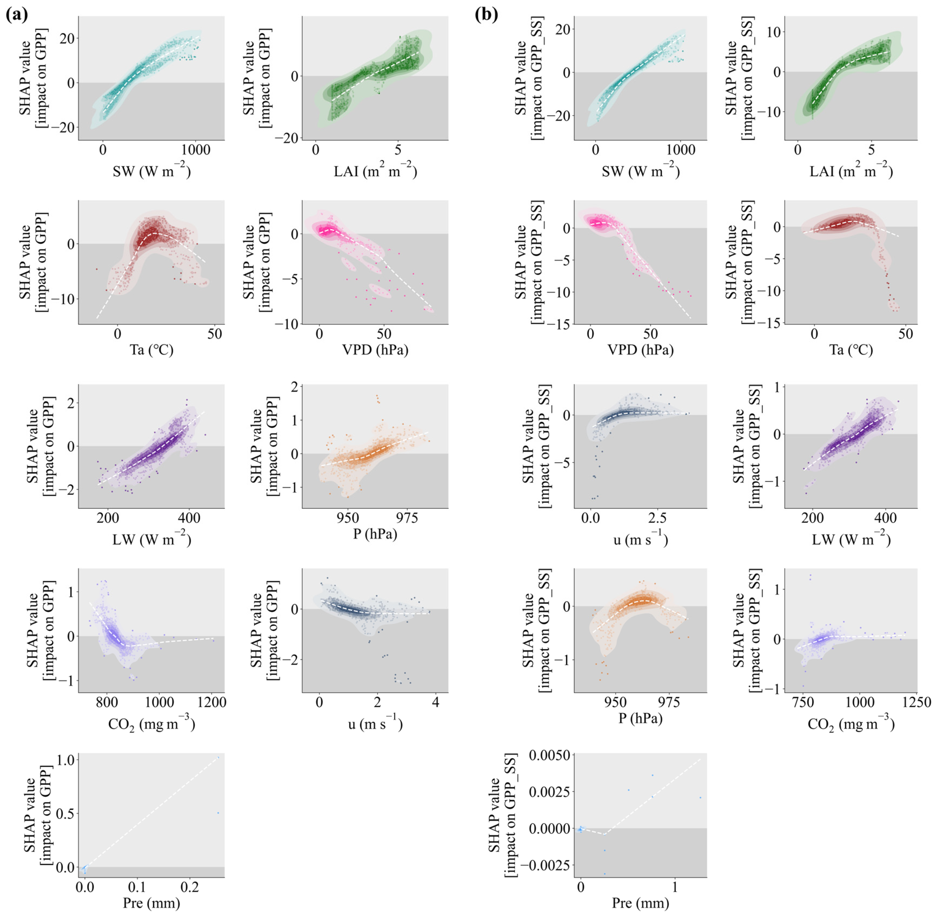
Figure A2. SHAP-based contribution of various factors to gross primary productivity (GPP) simulation under two scenarios: (a) a random forest (RF) model trained on observations; (b) an equivalent model trained on STEMMUS-SCOPE outputs. Note: identical colors indicate the same feature variables across panels.
Remotesensing 18 01364 g0a2
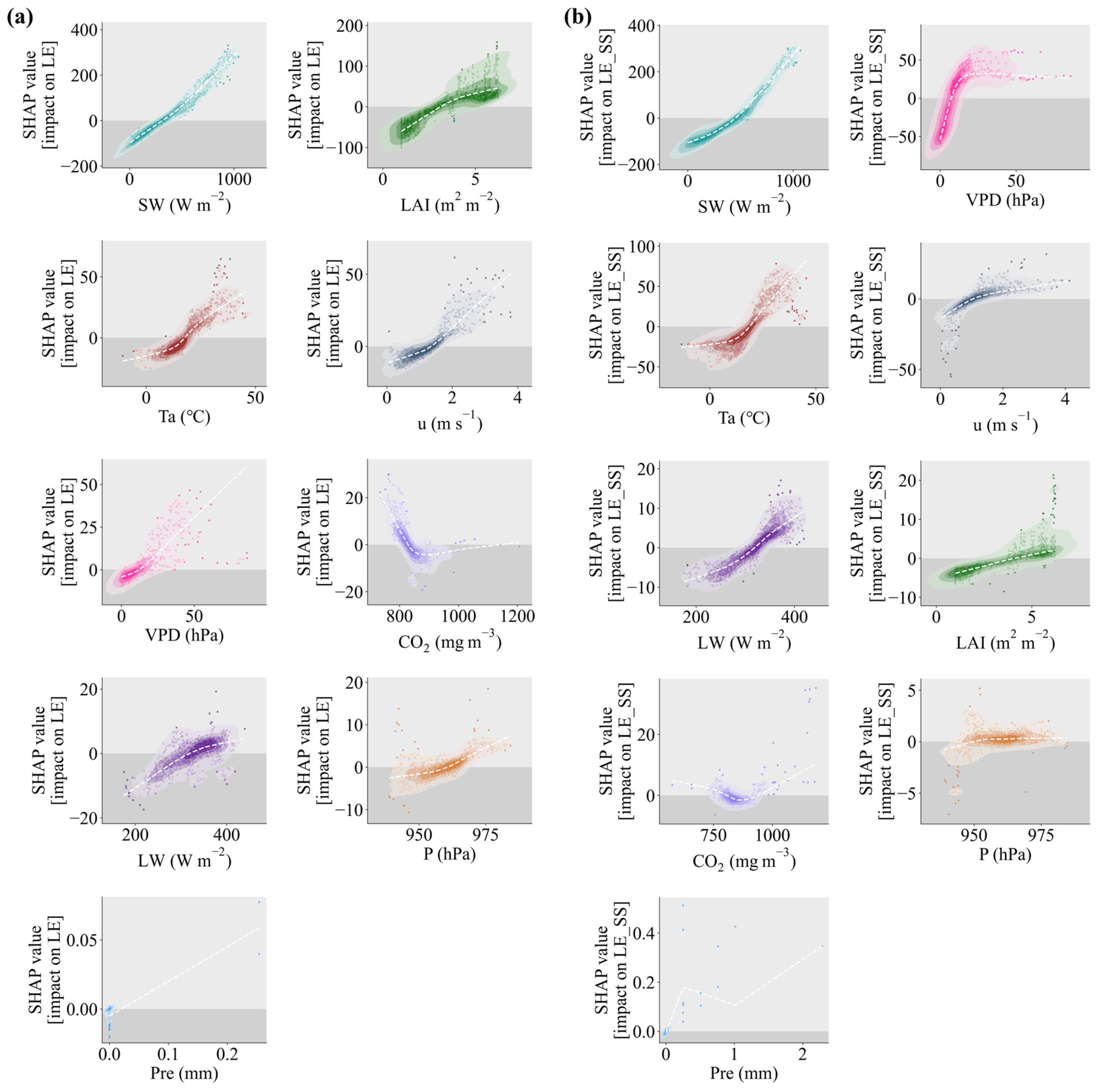
Figure A3. SHAP-based contribution of various factors to latent heat flux (LE) simulation under two scenarios: (a) a random forest (RF) model trained on observations; (b) an equivalent model trained on STEMMUS-SCOPE outputs. Note: identical colors indicate the same feature variables across panels.
Remotesensing 18 01364 g0a3
Figure A4. SHAP-based contribution of various factors to gross primary productivity (GPP) simulation under two scenarios: (a) a random forest (RF) model trained on observations; (b) an equivalent model trained on STEMMUS-MLR outputs. Note: identical colors indicate the same feature variables across panels.
Remotesensing 18 01364 g0a4
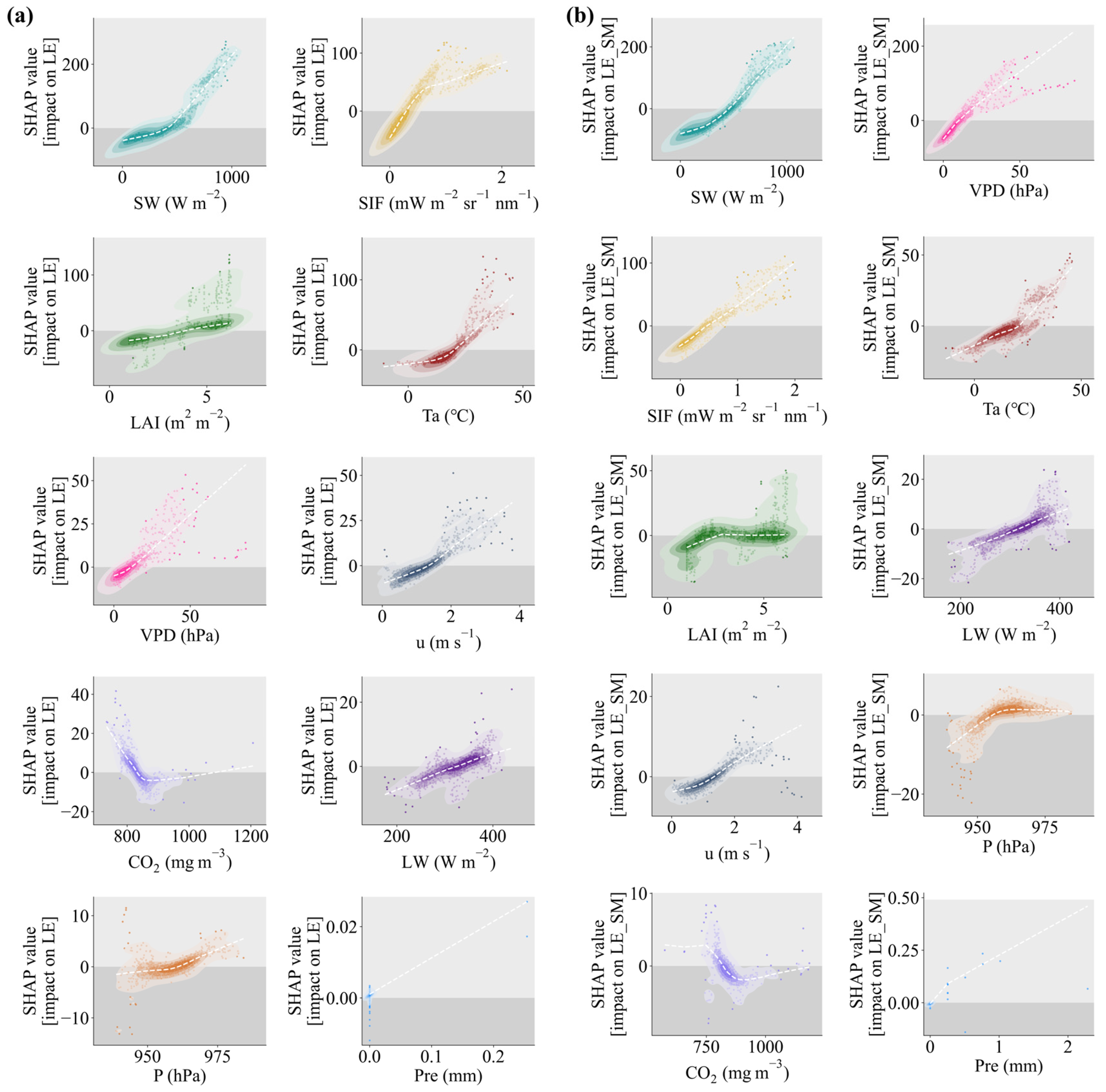
Figure A5. SHAP-based contribution of various factors to latent heat flux (LE) simulation under two scenarios: (a) a random forest (RF) model trained on observations; (b) an equivalent model trained on STEMMUS-MLR outputs. Note: identical colors indicate the same feature variables across panels.
Remotesensing 18 01364 g0a5
Figure A6. Comparison of Random Forest (RF)-based simulations of gross primary productivity (GPP) and latent heat flux (LE) using SS and SM results as inputs (SS means STEMMUS-SCOPE; SM means STEMMUS-MLR).
Remotesensing 18 01364 g0a6

References

  1. Kropp, H.; Ogle, K.; Vivoni, E.R.; Hultine, K.R. The sensitivity of evapotranspiration to inter-specific plant neighbor interactions: Implications for models. Ecosystems 2017, 20, 1311–1323. [Google Scholar] [CrossRef]
  2. Popović, N.; Petrone, R.M.; Green, A.; Khomik, M.; Price, J.S. Evolution of ecosystem-scale surface energy fluxes of a newly constructed boreal upland-fen watershed. Ecol. Eng. 2023, 194, 107059. [Google Scholar] [CrossRef]
  3. Zheng, C.; Jia, L.; Hu, G. Global land surface evapotranspiration monitoring by etmonitor model driven by multi-source satellite earth observations. J. Hydrol. 2022, 613, 128444. [Google Scholar] [CrossRef]
  4. Haghighi, E.; Kirchner, J.W. Near-surface turbulence as a missing link in modeling evapotranspiration-soil moisture relationships. Water Resour. Res. 2017, 53, 5320–5344. [Google Scholar] [CrossRef]
  5. Tarin, T.; Nolan, R.H.; Eamus, D.; Cleverly, J. Carbon and water fluxes in two adjacent australian semi-arid ecosystems. Agric. For. Meteorol. 2020, 281, 107853. [Google Scholar] [CrossRef]
  6. Xu, J.; Mu, Q.; Ding, Y.; Sun, S.; Zou, Y.; Yu, L.; Zhang, P.; Yang, N.; Guo, W.; Cai, H. Considering spatio-temporal dynamics of soil water with evapotranspiration partitioning helps to clarify water utilization characteristics of summer maize under deficit irrigation. J. Hydrol. 2023, 617, 129102. [Google Scholar] [CrossRef]
  7. Ruairuen, W.; Fochesatto, G.J.; Sparrow, E.B.; Schnabel, W.; Zhang, M.; Kim, Y. Evapotranspiration cycles in a high latitude agroecosystem: Potential warming role. PLoS ONE 2015, 10, e0137209. [Google Scholar] [CrossRef]
  8. Wang, W.; Xu, F.; Wang, J. Energy exchange and evapotranspiration over the ejina oasis riparian forest ecosystem with different land-cover types. Water 2021, 13, 3424. [Google Scholar] [CrossRef]
  9. Cavaleri, M.A.; Coble, A.P.; Ryan, M.G.; Bauerle, W.L.; Loescher, H.W.; Oberbauer, S.F. Tropical rainforest carbon sink declines during EI Nino as a result of reduced photosynthesis and increased respiration rates. New Phytol. 2017, 216, 136–149. [Google Scholar] [CrossRef] [PubMed]
  10. Kohonen, K.M.; Dewar, R.; Tramontana, G.; Mauranen, A.; Kolari, P.; Kooijmans, L.M.J.; Papale, D.; Vesala, T.; Mammarella, I. Intercomparison of methods to estimate gross primary production based on CO(2) and cos flux measurements. Biogeosciences 2022, 19, 4067–4088. [Google Scholar] [CrossRef] [PubMed]
  11. Boss, S.K.; Montana, Q.; Barnett, B. Global agriculture as an energy transfer system and the energy yield of world agriculture 1961–2013. Environ. Prog. Sustain. Energy 2017, 37, 108–121. [Google Scholar] [CrossRef]
  12. Amthor, J.S. After photosynthesis, what then: Importance of respiration to crop growth and yield. Field Crops Res. 2025, 321, 109638. [Google Scholar] [CrossRef]
  13. Nottingham, A.T.; Meir, P.; Velasquez, E.; Turner, B.L. Soil carbon loss by experimental warming in a tropical forest. Nature 2020, 584, 234. [Google Scholar] [CrossRef] [PubMed]
  14. Sun, P.; Wu, Y.; Xiao, J.; Hui, J.; Hu, J.; Zhao, F.; Qiu, L.; Liu, S. Remote sensing and modeling fusion for investigating the ecosystem water-carbon coupling processes. Sci. Total Environ. 2019, 697, 134064. [Google Scholar] [CrossRef] [PubMed]
  15. Gao, L.; Kang, S.; Bai, X.; Li, S.; Niu, J.; Ding, R. Water-carbon relationships and variations from the canopy to ecosystem scale in a sparse vineyard in the northwest china. J. Hydrol. 2021, 600, 126469. [Google Scholar] [CrossRef]
  16. Lawson, T.; Vialet-Chabrand, S. Speedy stomata, photosynthesis and plant water use efficiency. New Phytol. 2019, 221, 93–98. [Google Scholar] [CrossRef]
  17. Running, S.W.; Nemani, R.R.; Heinsch, F.A.; Zhao, M.S.; Reeves, M.; Hashimoto, H. A continuous satellite-derived measure of global terrestrial primary production. Bioscience 2004, 54, 547–560. [Google Scholar] [CrossRef]
  18. Yuan, W.; Liu, S.; Yu, G.; Bonnefond, J.-M.; Chen, J.; Davis, K.; Desai, A.R.; Goldstein, A.H.; Gianelle, D.; Rossi, F.; et al. Global estimates of evapotranspiration and gross primary production based on modis and global meteorology data. Remote Sens. Environ. 2010, 114, 1416–1431. [Google Scholar] [CrossRef]
  19. Bejagam, V.; Sharma, A. Remote sensing-based multi-scale characterization of ecohydrological indicators (ehis) in india. Ecol. Eng. 2023, 187, 106841. [Google Scholar] [CrossRef]
  20. Wang, Y. Exploring Terrestrial Eco-Hydrological Processes from Bottom-Up and Top-Down Perspectives. Ph.D. Thesis, Faculty of Geo-Information Science and Earth Observation (ITC), University of Twente, Enschede, The Netherlands, 2025. [Google Scholar]
  21. Raab, N.; Meza, F.J.; Franck, N.; Bambach, N. Empirical stomatal conductance models reveal that the isohydric behavior of an acacia caven mediterranean savannah scales from leaf to ecosystem. Agric. For. Meteorol. 2015, 213, 203–216. [Google Scholar] [CrossRef]
  22. Zeng, S.D.; Xia, J.; Chen, X.D.; Zou, L.; Du, H.; She, D.X. Integrated land-surface hydrological and biogeochemical processes in simulating water, energy and carbon fluxes over two different ecosystems. J. Hydrol. 2020, 582, 124390. [Google Scholar] [CrossRef]
  23. Li, Y.; Zhou, J.; Kinzelbach, W.; Cheng, G.; Li, X.; Zhao, W. Coupling a svat heat and water flow model, a stomatal-photosynthesis model and a crop growth model to simulate energy, water and carbon fluxes in an irrigated maize ecosystem. Agric. For. Meteorol. 2013, 176, 10–24. [Google Scholar] [CrossRef]
  24. Vote, C.; Hall, A.; Charlton, P. Carbon dioxide, water and energy fluxes of irrigated broad-acre crops in an australian semi-arid climate zone. Environ. Earth Sci. 2014, 73, 449–465. [Google Scholar] [CrossRef]
  25. Gu, X.Q.; Yao, L.; Wu, L.F. Prediction of water carbon fluxes and emission causes in rice paddies using two tree-based ensemble algorithms. Sustainability 2023, 15, 12333. [Google Scholar] [CrossRef]
  26. Scholze, M.; Buchwitz, M.; Dorigo, W.; Guanter, L.; Shaun, Q.G. Reviews and syntheses: Systematic earth observations for use in terrestrial carbon cycle data assimilation systems. Biogeosciences 2017, 14, 3401–3429. [Google Scholar] [CrossRef]
  27. Wang, Y.P.; Zhang, L.; Liang, X.; Yuan, W.P. Coupled models of water and carbon cycles from leaf to global: A retrospective and a prospective. Agric. For. Meteorol. 2024, 358, 110229. [Google Scholar] [CrossRef]
  28. Liu, X.; Peng, X.; Li, Y.; Gu, X.; Yu, L.; Wang, Y.; Cai, H. Environmental influences on evapotranspiration in wheat-maize rotation systems under diverse hydrological regimes in the Guanzhong Plain, China. Agric. Water Manag. 2024, 306, 109204. [Google Scholar] [CrossRef]
  29. Joetzjer, E.; Maignan, F.; Chave, J.; Goll, D.; Poulter, B.; Barichivich, J.; Maréchaux, I.; Luyssaert, S.; Guimberteau, M.; Naudts, K.; et al. Effect of tree demography and flexible root water uptake for modeling the carbon and water cycles of amazonia. Ecol. Model. 2022, 469, 109969. [Google Scholar] [CrossRef]
  30. He, X.; Liu, S.; Xu, T.; Yu, K.; Gentine, P.; Zhang, Z.; Xu, Z.; Jiao, D.; Wu, D. Improving predictions of evapotranspiration by integrating multi-source observations and land surface model. Agric. Water Manag. 2022, 272, 107827. [Google Scholar] [CrossRef]
  31. Ma, N.; Zhang, Y.; Xu, C.Y.; Szilagyi, J. Modeling actual evapotranspiration with routine meteorological variables in the data--scarce region of the tibetan plateau: Comparisons and implications. J. Geophys. Res. Biogeosci. 2015, 120, 1638–1657. [Google Scholar] [CrossRef]
  32. Li, W.; Duveiller, G.; Wieneke, S.; Forkel, M.; Gentine, P.; Reichstein, M.; Niu, S.; Migliavacca, M.; Orth, R. Regulation of the global carbon and water cycles through vegetation structural and physiological dynamics. Environ. Res. Lett. 2024, 19, 073008. [Google Scholar] [CrossRef]
  33. Ma, Y.M.; Guan, X.B.; Wang, Y.C.; Li, Y.Y.; Lin, D.K.; Shen, H.F. GPP estimation by transfer learning with combined solar-induced chlorophyll fluorescence and eddy covariance data. Int. J. Appl. Earth Obs. Geoinf. 2025, 139, 104503. [Google Scholar] [CrossRef]
  34. Raza, A.; Hu, Y.G.; Lu, Y.Z. Improving carbon flux estimation in tea plantation ecosystems: A machine learning ensemble approach. Eur. J. Agron. 2024, 160, 127297. [Google Scholar] [CrossRef]
  35. Xu, W.; Ma, L.; Ma, M.; Zhang, H.; Yuan, W. Spatial–temporal variability of snow cover and depth in the qinghai–tibetan plateau. J. Clim. 2017, 30, 1521–1533. [Google Scholar] [CrossRef]
  36. Zhang, T.L.; Sun, R.; Peng, C.H.; Zhou, G.Y.; Wang, C.L.; Zhu, Q.A.; Yang, Y.Z. Integrating a model with remote sensing observations by a data assimilation approach to improve the model simulation accuracy of carbon flux and evapotranspiration at two flux sites. Sci. China Earth Sci. 2016, 59, 337–348. [Google Scholar] [CrossRef]
  37. Zhao, G.; Bryan, B.A.; King, D.; Song, X.D.; Yu, Q. Parallelization and optimization of spatial analysis for large scale environmental model data assembly. Comput. Electron. Agric. 2012, 89, 94–99. [Google Scholar] [CrossRef]
  38. Sravani, C.; Kishore, P.; Jiang, J.H.; Rao, S.V.B. Climatological changes in soil moisture during the 21st century over the indian region using cmip5 and satellite observations. Remote Sens. 2022, 14, 2108. [Google Scholar] [CrossRef]
  39. Zeng, Y.; Verhoef, A.; Vereecken, H.; Ben-Dor, E.; Veldkamp, T.; Shaw, L.; Van Der Ploeg, M.; Wang, Y.; Su, Z. Monitoring and Modeling the Soil-Plant System Toward Understanding Soil Health. Rev. Geophys. 2025, 63, e2024RG000836. [Google Scholar] [CrossRef]
  40. Cai, W.Y.; Ullah, S.; Yan, L.; Lin, Y. Remote sensing of ecosystem water use efficiency: A review of direct and indirect estimation methods. Remote Sens. 2021, 13, 2393. [Google Scholar] [CrossRef]
  41. Gu, L.H.; Han, J.M.; Wood, J.D.; Chang, C.Y.Y.; Sun, Y. Sun-induced chl fluorescence and its importance for biophysical modeling of photosynthesis based on light reactions. New Phytol. 2019, 223, 1179–1191. [Google Scholar] [CrossRef]
  42. Mohammed, G.H.; Colombo, R.; Middleton, E.M.; Rascher, U.; van der Tol, C.; Nedbal, L.; Goulas, Y.; Pérez-Priego, O.; Damm, A.; Meroni, M.; et al. Remote sensing of solar-induced chlorophyll fluorescence (SIF) in vegetation: 50 years of progress. Remote Sens. Environ. 2019, 231, 111177. [Google Scholar] [CrossRef]
  43. Yang, J.; Lu, X.; Liu, Z.; Tang, X.; Yu, Q.; Wang, Y. Atmospheric drought dominates changes in global water use efficiency. Sci. Total Environ. 2024, 934, 173084. [Google Scholar] [CrossRef]
  44. Porcar-Castell, A.; Tyystjärvi, E.; Atherton, J.; van der Tol, C.; Flexas, J.; Pfündel, E.E.; Moreno, J.; Frankenberg, C.; Berry, J.A. Linking chlorophyll a fluorescence to photosynthesis for remote sensing applications: Mechanisms and challenges. J. Exp. Bot. 2014, 65, 4065–4095. [Google Scholar] [CrossRef]
  45. Meroni, M.; Rossini, M.; Guanter, L.; Alonso, L.; Rascher, U.; Colombo, R.; Moreno, J. Remote sensing of solar-induced chlorophyll fluorescence: Review of methods and applications. Remote Sens. Environ. 2009, 113, 2037–2051. [Google Scholar] [CrossRef]
  46. Yang, J.; Liu, Z.; Yu, Q.; Lu, X. Estimation of global transpiration from remotely sensed solar-induced chlorophyll fluorescence. Remote Sens. Environ. 2024, 303, 113998. [Google Scholar] [CrossRef]
  47. Frankenberg, C.; Fisher, J.B.; Worden, J.; Badgley, G.; Saatchi, S.S.; Lee, J.-E.; Toon, G.C.; Butz, A.; Jung, M.; Kuze, A.; et al. New global observations of the terrestrial carbon cycle from GOSAT: Patterns of plant fluorescence with gross primary productivity. Geophys. Res. Lett. 2011, 38, L17706. [Google Scholar] [CrossRef]
  48. Cai, G.; Lu, X.; Zhang, X.; Li, G.; Yu, H.; Lou, Z.; Fan, J.; Zhou, Y. Application of the Reconstructed Solar-Induced Chlorophyll Fluorescence by Machine Learning in Agricultural Drought Monitoring of Henan Province, China from 2010 to 2022. Agronomy 2024, 14, 1941. [Google Scholar] [CrossRef]
  49. Wang, Y.-Q.; Leng, P.; Shang, G.-F.; Zhang, X.; Li, Z.-L. Sun-induced chlorophyll fluorescence is superior to satellite vegetation indices for predicting summer maize yield under drought conditions. Comput. Electron. Agric. 2023, 205, 107615. [Google Scholar] [CrossRef]
  50. Yang, X.; Tang, J.; Mustard, J.F.; Lee, J.-E.; Rossini, M.; Joiner, J.; Munger, J.W.; Kornfeld, A.; Richardson, A.D. Solar-induced chlorophyll fluorescence that correlates with canopy photosynthesis on diurnal and seasonal scales in a temperate deciduous forest. Geophys. Res. Lett. 2015, 42, 2977–2987. [Google Scholar] [CrossRef]
  51. Sun, Y.; Frankenberg, C.; Wood, J.D.; Schimel, D.S.; Jung, M.; Guanter, L.; Drewry, D.T.; Verma, M.; Porcar-Castell, A.; Griffis, T.J.; et al. OCO-2 advances photosynthesis observation from space via solar-induced chlorophyll fluorescence. Science 2017, 358, eaam5747. [Google Scholar] [CrossRef]
  52. Chen, J.; Liu, X.; Ma, Y.; Liu, L. Effects of low temperature on the relationship between solar-induced chlorophyll fluorescence and gross primary productivity across different plant function types. Remote Sens. 2022, 14, 3716. [Google Scholar] [CrossRef]
  53. Bai, J.; Zhang, H.; Sun, R.; Li, X.; Xiao, J.; Wang, Y. Estimation of global GPP from GOME-2 and OCO-2 SIF by considering the dynamic variations of GPP-SIF relationship. Agric. For. Meteorol. 2022, 326, 109180. [Google Scholar] [CrossRef]
  54. Shan, N.; Ju, W.; Migliavacca, M.; Martini, D.; Guanter, L.; Chen, J.; Goulas, Y.; Zhang, Y. Modeling canopy conductance and transpiration from solar-induced chlorophyll fluorescence. Agric. For. Meteorol. 2019, 268, 189–201. [Google Scholar] [CrossRef]
  55. Damm, A.; Haghighi, E.; Paul-Limoges, E.; van der Tol, C. On the seasonal relation of sun-induced chlorophyll fluorescence and transpiration in a temperate mixed forest. Agric. For. Meteorol. 2021, 304–305, 108386. [Google Scholar] [CrossRef]
  56. Wang, Y.; Zeng, Y.; Yu, L.; Yang, P.; Van der Tol, C.; Yu, Q.; Lü, X.; Cai, H.; Su, Z. Integrated modeling of canopy photosynthesis, fluorescence, and the transfer of energy, mass, and momentum in the soil–plant–atmosphere continuum (stemmus–scope v1.0.0). Geosci. Model Dev. 2021, 14, 1379–1407. [Google Scholar] [CrossRef]
  57. Tang, E.; Zeng, Y.; Wang, Y.; Song, Z.; Yu, D.; Wu, H.; Qiao, C.; van der Tol, C.; Du, L.; Su, Z. Understanding the effects of revegetated shrubs on fluxes of energy, water, and gross primary productivity in a desert steppe ecosystem using the stemmus–scope model. Biogeosciences 2024, 21, 893–909. [Google Scholar] [CrossRef]
  58. Abramowitz, G.; Ukkola, A.; Hobeichi, S.; Cranko Page, J.; Lipson, M.; De Kauwe, M.G.; Green, S.; Brenner, C.; Frame, J.; Nearing, G.; et al. On the predictability of turbulent fluxes from land: Plumber2 mip experimental description and preliminary results. Biogeosciences 2024, 21, 5517–5538. [Google Scholar] [CrossRef]
  59. Wang, Y.F.; Zeng, Y.J.; Alidoost, F.; Schilperoort, B.; Song, Z.J.; Yu, D.Y.; Tang, E.T.; Han, Q.Q.; Liu, Z.Q.; Peng, X.B.; et al. A physically consistent dataset of water-energy-carbon fluxes across the soil-plant-atmosphere continuum. Sci. Data 2025, 12, 1146. [Google Scholar] [CrossRef]
  60. Wang, Y.; Zeng, Y.; Su, Z. Data Underlying the Research on Advancing the Understanding of Eco-Hydrological Processes with the Stemmus-MLR Model. 4TU.ResearchData. 2025. Available online: https://doi.org/10.4121/0feee349-83e7-4872-8fd4-bc07aa4dd265.v1 (accessed on 9 July 2025).
  61. Liu, Z.; Zhao, F.; Liu, X.; Yu, Q.; Wang, Y.; Peng, X.; Cai, H.; Lu, X. Direct estimation of photosynthetic CO2 assimilation from solar-induced chlorophyll fluorescence (SIF). Remote Sens. Environ. 2022, 271, 112893. [Google Scholar] [CrossRef]
  62. Peng, X.; Liu, X.; Wang, Y.; Cai, H. Evapotranspiration partitioning and estimation based on crop coefficients of winter wheat cropland in the guanzhong plain, china. Agronomy 2023, 13, 2982. [Google Scholar] [CrossRef]
  63. Zheng, J.; Wang, H.; Fan, J.; Zhang, F.; Guo, J.; Liao, Z.; Zhuang, Q. Wheat straw mulching with nitrification inhibitor application improves grain yield and economic benefit while mitigating gaseous emissions from a dryland maize field in northwest china. Field Crops Res. 2021, 265, 108125. [Google Scholar] [CrossRef]
  64. Chen, H.; Hou, H.-J.; Wang, X.-Y.; Zhu, Y.; Saddique, Q.; Wang, Y.-F.; Cai, H. The effects of aeration and irrigation regimes on soil CO2 and N2O emissions in a greenhouse tomato production system. J. Integr. Agric. 2018, 17, 449–460. [Google Scholar] [CrossRef]
  65. Wang, Y.; Cai, H.; Yu, L.; Peng, X.; Xu, J.; Wang, X. Evapotranspiration partitioning and crop coefficient of maize in dry semi-humid climate regime. Agric. Water Manag. 2020, 236, 106164. [Google Scholar] [CrossRef]
  66. Wang, Y.; Zou, Y.; Cai, H.; Zeng, Y.; He, J.; Yu, L.; Zhang, C.; Saddique, Q.; Peng, X.; Siddique, K.H.M.; et al. Seasonal variation and controlling factors of evapotranspiration over dry semi-humid cropland in guanzhong plain, china. Agric. Water Manag. 2022, 259, 107242. [Google Scholar] [CrossRef]
  67. Yu, L.; Zeng, Y.; Su, Z.; Cai, H.; Zheng, Z. The effect of different evapotranspiration methods on portraying soil water dynamics and et partitioning in a semi-arid environment in northwest china. Hydrol. Earth Syst. Sci. 2016, 20, 975–990. [Google Scholar] [CrossRef]
  68. Zhou, X.; Liu, Z.; Xu, S.; Zhang, W.; Wu, J. An Automated Comparative Observation System for Sun-Induced Chlorophyll Fluorescence of Vegetation Canopies. Sensors 2016, 16, 775. [Google Scholar] [CrossRef]
  69. Liu, Z.; Guo, C.; Yu, Q.; Zhu, P.; Peng, X.; Dong, M.; Cai, H.; Lu, X. A SIF-based approach for quantifying canopy photosynthesis by simulating the fraction of open PSII reaction centers (qL). Remote Sens. Environ. 2024, 305, 114111. [Google Scholar] [CrossRef]
  70. Meroni, M.; Picchi, V.; Rossini, M.; Cogliati, S.; Panigada, C.; Nali, C.; Lorenzini, G.; Colombo, R. Leaf level early assessment of ozone injuries by passive fluorescence and photochemical reflectance index. Int. J. Remote Sens. 2008, 29, 5409–5422. [Google Scholar] [CrossRef]
  71. Liu, X.J.; Liu, Z.Q.; Liu, L.Y.; Lu, X.L.; Chen, J.D.; Du, S.S.; Zou, C. Modelling the influence of incident radiation on the SIF-based GPP estimation for maize. Agric. For. Meteorol. 2021, 307, 108522. [Google Scholar] [CrossRef]
  72. Yang, K.; Ryu, Y.; Dechant, B.; Berry, J.A.; Hwang, Y.; Jiang, C.; Kang, M.; Kim, J.; Kimm, H.; Kornfeld, A.; et al. Sun-induced chlorophyll fluorescence is more strongly related to absorbed light than to photosynthesis at half-hourly resolution in a rice paddy. Remote Sens. Environ. 2018, 216, 658–673. [Google Scholar] [CrossRef]
  73. Chang, C.Y.; Guanter, L.; Frankenberg, C.; Köhler, P.; Gu, L.H.; Magney, T.S.; Grossmann, K.; Sun, Y. Systematic assessment of retrieval methods for canopy far-red solar-induced chlorophyll fluorescence using high-frequency automated field spectroscopy. J. Geophys. Res. Biogeosci. 2020, 125, e2019JG005533. [Google Scholar] [CrossRef]
  74. Guanter, L.; Frankenberg, C.; Dudhia, A.; Lewis, P.E.; Gómez-Dans, J.; Kuze, A.; Suto, H.; Grainger, R.G. Retrieval and global assessment of terrestrial chlorophyll fluorescence from GOSAT space measurements. Remote Sens. Environ. 2012, 121, 236–251. [Google Scholar] [CrossRef]
  75. Guanter, L.; Rossini, M.; Colombo, R.; Meroni, M.; Frankenberg, C.; Lee, J.E.; Joiner, J. Using field spectroscopy to assess the potential of statistical approaches for the retrieval of sun-induced chlorophyll fluorescence from ground and space. Remote Sens. Environ. 2013, 133, 52–61. [Google Scholar] [CrossRef]
  76. Zhang, Z.; Zhang, X.; Porcar-Castell, A.; Chen, J.M.; Ju, W.; Wu, L.; Wu, Y.; Zhang, Y. Sun-induced chlorophyll fluorescence is more strongly related to photosynthesis with hemispherical than nadir measurements: Evidence from field observations and model simulations. Remote Sens. Environ. 2022, 279, 113118. [Google Scholar] [CrossRef]
  77. Wutzler, T.; Lucas-Moffat, A.; Migliavacca, M.; Knauer, J.; Sickel, K.; Sigut, L.; Menzer, O.; Reichstein, M. Basic and extensible post-processing of eddy covariance flux data with REddyProc. Biogeosciences 2018, 15, 5015–5030. [Google Scholar] [CrossRef]
  78. Campbell, G.S.; Norman, J.M. An Introduction to Environmental Biophysics; Springer Science & Business Media: Berlin/Heidelberg, Germany, 1977. [Google Scholar]
  79. Zeng, Y.J.; Su, Z.B.; Wan, L.; Wen, J. A simulation analysis of the advective effect on evaporation using a two-phase heat and mass flow model. Water Resour. Res. 2011, 47, W10529. [Google Scholar] [CrossRef]
  80. Zeng, Y.J.; Su, Z.B.; Wan, L.; Wen, J. Numerical analysis of air-water-heat flow in unsaturated soil: Is it necessary to consider airflow in land surface models? J. Geophys. Res. Atmos. 2011, 116, D20107. [Google Scholar] [CrossRef]
  81. Yu, L.Y.; Zeng, Y.J.; Wen, J.; Su, Z.B. Liquid-vapor-air flow in the frozen soil. J. Geophys. Res. Atmos. 2018, 123, 7393–7415. [Google Scholar] [CrossRef]
  82. Zeng, Y.; Su, Z. Stemmus: Simultaneous Transfer of Energy, Mass and Momentum in Unsaturated Soil; University of Twente, Faculty of Geo-Information Science and Earth Observation (ITC): Enschede, The Netherlands, 2013. [Google Scholar]
  83. Meyer, H.; Reudenbach, C.; Wöllauer, S.; Nauss, T. Importance of spatial predictor variable selection in machine learning applications—Moving from data reproduction to spatial prediction. Ecol. Model. 2019, 411, 108815. [Google Scholar] [CrossRef]
  84. Reitz, O.; Graf, A.; Schmidt, M.; Ketzler, G.; Leuchner, M. Upscaling net ecosystem exchange over heterogeneous landscapes with machine learning. J. Geophys. Res. Biogeosci. 2021, 126, e2020JG005814. [Google Scholar] [CrossRef]
  85. Zhang, C.; Luo, G.; Hellwich, O.; Chen, C.; Zhang, W.; Xie, M.; He, H.; Shi, H.; Wang, Y. A framework for estimating actual evapotranspiration at weather stations without flux observations by combining data from modis and flux towers through a machine learning approach. J. Hydrol. 2021, 603, 127047. [Google Scholar] [CrossRef]
  86. Zahura, F.T.; Goodall, J.L. Predicting combined tidal and pluvial flood inundation using a machine learning surrogate model. J. Hydrol. Reg. Stud. 2022, 41, 101087. [Google Scholar] [CrossRef]
  87. Zahura, F.T.; Goodall, J.L.; Sadler, J.M.; Shen, Y.W.; Morsy, M.M.; Behl, M. Training machine learning surrogate models from a high-fidelity physics-based model: Application for real-time street-scale flood prediction in an urban coastal community. Water Resour. Res. 2020, 56, e2019WR027038. [Google Scholar] [CrossRef]
  88. Lundberg, S.M.; Erion, G.; Chen, H.; DeGrave, A.; Prutkin, J.M.; Nair, B.; Katz, R.; Himmelfarb, J.; Bansal, N.; Lee, S.I. From local explanations to global understanding with explainable AI for trees. Nat. Mach. Intell. 2020, 2, 56–67. [Google Scholar] [CrossRef]
  89. Yan, Y.L.; Li, B.L.; Dechant, B.; Xu, M.Z.; Luo, X.Z.; Qu, S.; Miao, G.F.; Leng, J.Y.; Shang, R.; Shu, L.; et al. Plant traits shape global spatiotemporal variations in photosynthetic efficiency. Nat. Plants 2025, 11, 924–934. [Google Scholar] [CrossRef] [PubMed]
  90. Huan, S. Shapelet-based decomposition stack machine learning model explains more middle river reaches water level hydrological process with high accuracy early warning. J. Hydrol. 2025, 662, 133927. [Google Scholar] [CrossRef]
  91. Samantaray, S.; Sahoo, A.; Yaseen, Z.M.; Al-Suwaiyan, M.S. River discharge prediction based multivariate climatological variables using hybridized long short-term memory with nature inspired algorithm. J. Hydrol. 2025, 649, 132453. [Google Scholar] [CrossRef]
  92. Qiu, R.; Han, G.; Li, X.; Xiao, J.; Liu, J.; Wang, S.; Li, S.; Gong, W. Contrasting responses of relationship between solar-induced fluorescence and gross primary production to drought across aridity gradients. Remote Sens. Environ. 2024, 302, 113984. [Google Scholar] [CrossRef]
  93. van der Tol, C.; Berry, J.A.; Campbell, P.K.E.; Rascher, U. Models of fluorescence and photosynthesis for interpreting measurements of solar-induced chlorophyll fluorescence. J. Geophys. Res. Biogeosci. 2014, 119, 2312–2327. [Google Scholar] [CrossRef]
  94. Fisher, J.B.; Tu, K.P.; Baldocchi, D.D. Global estimates of the land-atmosphere water flux based on monthly avhrr and islscp-ii data, validated at 16 fluxnet sites. Remote Sens. Environ. 2008, 112, 901–919. [Google Scholar] [CrossRef]
  95. Huang, J.Y.; Sehgal, V.; Alvarez, L.V.; Brocca, L.; Cai, S.H.; Cheng, R.; Cheng, X.H.; Du, J.Y.; El Masri, B.; Endsley, K.A.; et al. Remotely sensed high-resolution soil moisture and evapotranspiration: Bridging the gap between science and society. Water Resour. Res. 2025, 61, e2024WR037929. [Google Scholar] [CrossRef]
  96. Pan, S.F.; Pan, N.Q.; Tian, H.Q.; Friedlingstein, P.; Sitch, S.; Shi, H.; Arora, V.K.; Haverd, V.; Jain, A.K.; Kato, E.; et al. Evaluation of global terrestrial evapotranspiration using state-of-the-art approaches in remote sensing, machine learning and land surface modeling. Hydrol. Earth Syst. Sci. 2020, 24, 1485–1509. [Google Scholar] [CrossRef]
  97. Shan, N.; Zhang, Y.; Chen, J.M.; Ju, W.; Migliavacca, M.; Peñuelas, J.; Yang, X.; Zhang, Z.; Nelson, J.A.; Goulas, Y. A model for estimating transpiration from remotely sensed solar-induced chlorophyll fluorescence. Remote Sens. Environ. 2021, 252, 112134. [Google Scholar] [CrossRef]
  98. Zhang, Q.; Liu, X.; Zhou, K.; Zhou, Y.; Gentine, P.; Pan, M.; Katul, G.G. Solar-induced chlorophyll fluorescence sheds light on global evapotranspiration. Remote Sens. Environ. 2024, 305, 114061. [Google Scholar] [CrossRef]
  99. Bu, J.; Gan, G.; Chen, J.; Su, Y.; Yuan, M.; Gao, Y.; Domingo, F.; López-Ballesteros, A.; Migliavacca, M.; El-Madany, T.S.; et al. Dryland evapotranspiration from remote sensing solar-induced chlorophyll fluorescence: Constraining an optimal stomatal model within a two-source energy balance model. Remote Sens. Environ. 2024, 303, 113999. [Google Scholar] [CrossRef]
  100. Xue, K.J.; Song, L.S.; Xu, Y.H.; Liu, S.M.; Zhao, G.L.; Tao, S.N.; Magliulo, E.; Manco, A.; Liddell, M.; Wohlfahrt, G.; et al. Estimating ecosystem evaporation and transpiration using a soil moisture coupled two-source energy balance model across fluxnet sites. Agric. For. Meteorol. 2023, 337, 109513. [Google Scholar] [CrossRef]
  101. Caine, R.S.; Khan, M.S.; Brench, R.A.; Walker, H.J.; Croft, H.L. Inside-out: Synergising leaf biochemical traits with stomatal-regulated water fluxes to enhance transpiration modelling during abiotic stress. Plant Cell Environ. 2024, 47, 3494–3513. [Google Scholar] [CrossRef]
  102. Jonard, F.; De Cannière, S.; Brüggemann, N.; Gentine, P.; Short Gianotti, D.J.; Lobet, G.; Miralles, D.G.; Montzka, C.; Pagán, B.R.; Rascher, U.; et al. Value of sun-induced chlorophyll fluorescence for quantifying hydrological states and fluxes: Current status and challenges. Agric. For. Meteorol. 2020, 291, 108088. [Google Scholar] [CrossRef]
  103. Wang, R.; Qin, X.; Du, Z.; Liu, Y.; Zhao, Q.; Jin, Z.; Qiang, D. Improving terrestrial evapotranspiration estimation using physics-guided machine learning model driven by solar-induced chlorophyll fluorescence. J. Hydrol. 2025, 661, 133468. [Google Scholar] [CrossRef]
  104. Zhang, K.; Kimball, J.S.; Running, S.W. A review of remote sensing based actual evapotranspiration estimation. Wiley Interdiscip. Rev. Water 2016, 3, 834–853. [Google Scholar] [CrossRef]
  105. Chen, H.; Huang, J.J.; Dash, S.S.; Wei, Y.; Li, H. A hybrid deep learning framework with physical process description for simulation of evapotranspiration. J. Hydrol. 2022, 606, 127422. [Google Scholar] [CrossRef]
  106. Zhang, T.; Liang, Z.; Zhou, J.; Shao, Q.; Sarukkalige, R.; Lü, H.; Zhang, J.; Bi, C.; Wang, J.; Hu, Y.; et al. Multi-layer grid-scale soil moisture estimation using spatiotemporal deep learning methods with physical constraints. J. Hydrol. 2025, 657, 133086. [Google Scholar] [CrossRef]
  107. Abbes, A.B.; Jarray, N.; Farah, I.R. Advances in remote sensing based soil moisture retrieval: Applications, techniques, scales and challenges for combining machine learning and physical models. Artif. Intell. Rev. 2024, 57, 224. [Google Scholar] [CrossRef]
  108. Chen, H.; Ghani Razaqpur, A.; Wei, Y.; Huang, J.J.; Li, H.; McBean, E. Estimation of global land surface evapotranspiration and its trend using a surface energy balance constrained deep learning model. J. Hydrol. 2023, 627, 130224. [Google Scholar] [CrossRef]
  109. He, X.L.; Liu, S.M.; Bateni, S.M.; Xu, T.R.; Jun, C.; Kim, D.; Li, X.; Song, L.S.; Zhao, L.; Xu, Z.W.; et al. Innovative approach for estimating evapotranspiration and gross primary productivity by integrating land data assimilation, machine learning, and multi-source observations. Agric. For. Meteorol. 2024, 355, 110136. [Google Scholar] [CrossRef]
  110. Collatz, G.J.; Ball, J.T.; Grivet, C.; Berry, J.A. Physiological and environmental regulation of stomatal conductance, photosynthesis and transpiration. Agric. For. Meteorol. 1991, 54, 107–136. [Google Scholar] [CrossRef]
  111. Collatz, G.J.; Ribas-Carbo, M.; Berry, J.A. Coupled photosynthesis-stomatal conductance model for leaves of C4 plants. Aust. J. Plant Physiol. 1992, 19, 519–538. [Google Scholar] [CrossRef]
  112. Farquhar, G.D.; von Caemmerer, S.; Berry, J.A. A biochemical model of photosynthetic CO2 assimilation in leaves of C3 species. Planta 1980, 149, 78–90. [Google Scholar] [CrossRef]
  113. Bayat, B.; van der Tol, C.; Yang, P.; Verhoef, W. Extending the scope model to combine optical reflectance and soil moisture observations for remote sensing of ecosystem functioning under water stress conditions. Remote Sens. Environ. 2019, 221, 286–301. [Google Scholar] [CrossRef]
  114. van Genuchten, M.T. A closed-form equation for predicting the hydraulic conductivity of unsaturated soils. Soil. Sci. Soc. Am. J. 1980, 44, 892–898. [Google Scholar] [CrossRef]
  115. Reid, J.B.; Huck, M.G. Diurnal variation of crop hydraulic resistance: A new analysis. Agron. J. 1990, 82, 827–834. [Google Scholar] [CrossRef]
  116. Klepper, B.; Rickman, R.W.; Taylor, H.M. Farm management and the function of field crop root systems. Agric. Water Manag. 1983, 7, 115–141. [Google Scholar] [CrossRef]
  117. Pfündel, E. Estimating the contribution of photosystem I to total leaf chlorophyll fluorescence. Photosynth. Res. 1998, 56, 185–195. [Google Scholar] [CrossRef]
  118. Zhang, Z.; Chen, J.M.; Guanter, L.; He, L.; Zhang, Y. From canopy-leaving to total canopy far-red fluorescence emission for remote sensing of photosynthesis: First results from tropomi. Geophys. Res. Lett. 2019, 46, 12030–12040. [Google Scholar] [CrossRef]
  119. Badgley, G.; Field, C.B.; Berry, J.A. Canopy near-infrared reflectance and terrestrial photosynthesis. Sci. Adv. 2017, 3, e1602244. [Google Scholar] [CrossRef]
  120. Katul, G.; Manzoni, S.; Palmroth, S.; Oren, R. A stomatal optimization theory to describe the effects of atmospheric CO2 on leaf photosynthesis and transpiration. Ann. Bot. 2010, 105, 431–442. [Google Scholar] [CrossRef]
  121. Medlyn, B.E.; Duursma, R.A.; Eamus, D.; Ellsworth, D.S.; Prentice, I.C.; Barton, C.V.M.; Crous, K.Y.; De Angelis, P.; Freeman, M.; Wingate, L. Reconciling the optimal and empirical approaches to modelling stomatal conductance. Glob. Change Biol. 2011, 17, 2134–2144. [Google Scholar] [CrossRef]
  122. Wang, Y.P.; Leuning, R. A two-leaf model for canopy conductance, photosynthesis and partitioning of available energy I:: Model description and comparison with a multi-layered model. Agric. For. Meteorol. 1998, 91, 89–111. [Google Scholar] [CrossRef]
Figure 1. Location of the Yangling flux site in a cropland region of China. (a) Location of Shaanxi Province in China and the Guanzhong Plain within Shaanxi Province. (b) Vegetation types across the Guanzhong Plain and the specific location of the Yangling Site.
Remotesensing 18 01364 g001
Figure 2. Schematic diagram of the overall workflow of this study (Ta: Air Temperature, u: Wind Speed, Pre: Precipitation, SW: Shortwave Radiation, LW: Longwave Radiation, VPD: Vapor Pressure Deficit, P: Air Pressure, CO2: Carbon Dioxide Concentration, LAI: Leaf Area Index, SIF: Solar-Induced Chlorophyll Fluorescence, NDVI: Normalized Difference Vegetation Index, NIRv: Near-Infrared Reflectance of Vegetation, ET: Evapotranspiration, RF: Random Forest, and SHAP: Shapley additive explanations).
Remotesensing 18 01364 g002
Figure 3. Variation of air temperature (Ta), wind speed (u), shortwave radiation (SW), solar-induced chlorophyll fluorescence (SIF), longwave radiation (LW), vapor pressure deficit (VPD), air pressure (P), CO2 concentration, precipitation (Pre), Leaf area index (LAI), gross primary productivity (GPP), and latent heat flux (LE) at the wheat cropland of the Yangling station.
Remotesensing 18 01364 g003
Figure 4. Comparison between in-situ observations (GPP_o, LE_o) and simulations (GPP_m, LE_m) of gross primary productivity (GPP) and latent heat flux (LE) by STEMMUS-SCOPE.
Remotesensing 18 01364 g004
Figure 5. Comparison between in-situ observations (GPP_o, LE_o) and simulations (GPP_m, LE_m) of gross primary productivity (GPP) and latent heat flux (LE) by STEMMUS-MLR.
Remotesensing 18 01364 g005
Figure 6. SHAP-based explanatory power of various factors in estimating gross primary productivity (GPP) and latent heat flux (LE): meteorological variables only (top) and meteorological variables with solar-induced chlorophyll fluorescence (SIF) (bottom).
Remotesensing 18 01364 g006
Figure 7. Comparison of Random Forest (RF)-based simulations of gross primary productivity (GPP) and latent heat flux (LE), with and without solar-induced chlorophyll fluorescence (SIF) as a feather.
Remotesensing 18 01364 g007
Figure 8. SHAP-based contribution to gross primary productivity (GPP) simulation under two variable combinations: (a) meteorological variables only (without solar-induced chlorophyll fluorescence, SIF); (b) meteorological variables plus SIF. Note: identical colors indicate the same feature variables across panels.
Remotesensing 18 01364 g008
Figure 9. SHAP-based contribution to latent heat flux (LE) simulation under two variable combinations: (a) meteorological variables only (without solar-induced chlorophyll fluorescence, SIF); (b) meteorological variables plus SIF. Note: identical colors indicate the same feature variables across panels.
Remotesensing 18 01364 g009
Figure 10. SHAP-based explanatory power of various factors in estimating gross primary productivity (GPP)and latent heat flux (LE) using SS and SM results as inputs: SS (top) and SM (bottom). SS indicates STEMMUS-SCOPE and SM indicates STEMMUS-MLR.
Remotesensing 18 01364 g010
Disclaimer/Publisher’s Note: The statements, opinions and data contained in all publications are solely those of the individual author(s) and contributor(s) and not of MDPI and/or the editor(s). MDPI and/or the editor(s) disclaim responsibility for any injury to people or property resulting from any ideas, methods, instructions or products referred to in the content.