Potato Late Blight Disease Detection on UAV Multispectral Imagery

Highlights

What are the main findings?

• A Mask R-CNN model with a ResNeXt-101 backbone achieved the best performance (F1-score = 84.2%) in potato plant detection when transfer learning was applied using a Mask R-CNN model pretrained on apple orchard data.
• A DINOv3-based Mask R-CNN achieved the best performance (F1-score = 69.0%) in plant health classification despite the limited number of labelled samples, which reflects realistic field conditions in UAV-based potato late blight disease detection studies.
• A decision tree machine learning (ML) algorithm applied to vegetation indices achieved the best performance (F1-score = 66.7%).
• Red-edge and chlorophyll-related vegetation indices were the most discriminative features.

What are the implications of the main findings?

• UAV multispectral imagery enables effective detection of potato late blight at the plant level.
• Red-edge-based vegetation indices play a key role in capturing disease-induced physiological changes.
• Both deep learning (DL) and combined DL-ML approaches provide scalable solutions for potato late blight disease monitoring.

Abstract

In this study, Mask R-CNN was applied to 5-band raw reflectance images to detect potato plants in UAV images. The highest model performance across all metrics was achieved with a ResNeXt-101 backbone and transfer learning from the same model trained on apple orchard data. An F-1 score of 84.2% was achieved. To determine whether the plant was infected with PLB, two methods were used. In the first method, a Mask R-CNN with a DINOv3 small variant backbone was applied to 5-band raw reflectance images. The highest achieved F1-score was 69.05%. In the second method, classical ML classifiers were applied to the 5-band raw reflectance images and 16 associated vegetation index images. The highest F1-score (66.71%) was obtained with a decision tree classifier applied to the 16 vegetation index images. Feature importance analysis indicated that chlorophyll- and red-edge-related indices, such as CIgreen, TCARI, OSAVI2, and Red-edge NDVI, were the most discriminative features for distinguishing healthy and unhealthy potato plants. These results show the effectiveness of combining deep learning and machine learning approaches for potato late blight detection using UAV multispectral imagery.

1. Introduction

Potato late blight is one of the most economically damaging diseases for potato crops, affecting yield quality and quantity worldwide. Early detection and accurate classification of this disease are crucial for minimizing crop loss and supporting effective management strategies. Traditional PLB detection methods, like manual field inspections, are labour-intensive, time-consuming, and often inconsistent, leading to inaccurate assessments. Remote sensing technologies, particularly UAVs equipped with multispectral and hyperspectral cameras, have emerged as a powerful, cost-effective alternative. UAVs can capture spectral information across large areas, including wavelengths beyond the visible spectrum, which is essential for analyzing plant health indicators. This aerial perspective enables early PLB detection across entire fields, enhancing both efficiency and the scale of monitoring efforts. To effectively use these images for plant disease detection, it is necessary to have strong image processing methods, such as ML algorithms, especially convolutional neural networks (CNNs) and other deep learning models.

Most studies testing advanced image processing methods for detecting potato late blight disease primarily use ground-level images of the canopy [1] or at the leaf level [1,2,3,4,5,6,7,8,9,10,11]. Only a few studies used UAV imagery to detect PLB-infected plants.

Table 1. Accuracy Comparison of Models for Potato Late Blight Classification Using UAV Imagery.

Imagery Type	Input Feature *	Method	Accuracy (%)	Region	Pixel Size (cm)	Classes	Reference
RGB + NIR	NDVI	NDVI thresholds	91.00	Scotland	1.0	Healthy, Infected	[12]
Hyperspectral	Raw Reflectance	Random Forest	99.00	Portugal	4.0	Healthy, Infected, Road, Shadow, Soil, Weeds	[13]
		CropdocNet	95.75	China	2.5	Healthy, Infected, Soil, Background	[14]
Multispectral	Mean-Red, Contrast-Red, MSAVI	Random Forest	97.50	China	1.1	Healthy, Mild, Moderate, Severe Late Blight	[15]
	Raw Reflectance	Random Forest	93.00	Portugal	4.0	Healthy, Infected, Road, Shadow, Soil, Weeds	[13]
	Red, Green, Blue, NIR, Red-Edge, NDVI, NDRE, NDVI textures, NIR textures	Random Forest	81.02	Peru	3.4	11 classes of disease severity (Increasing 10% of the affected leaf area), Soil	[16]

* See details of the abbreviations in the abbreviation list.

compares the classification accuracies reported by recent studies using UAV imagery for PLB disease detection. Only one study used images acquired by an RGB camera and a near-infrared sensor. The images were combined into NDVI images, and using NDVI thresholds, 91.00% accuracy was achieved in distinguishing between healthy and infected plants [12]. The other studies employed hyperspectral or multispectral imagery. With hyperspectral imagery, the highest accuracy (99%) was achieved when Random Forest was used to classify the images into the following classes: healthy and infected plants, roads, shadows, soil, and weeds [13]. Ref. [14] achieved 95.75% accuracy when they developed a model, called CropdocNet, combining convolutional neural networks and capsule layers to detect infected and healthy plants. In the case of multispectral imagery, all the studies used Random Forests as the classifier. The best accuracy was achieved by [15] (97.5%), when the classifier was applied to such Mean-Red, Contrast-Red, and MSAVI images to detect plants with various PLB severities. In addition, several studies have shown that vegetation indices derived from multispectral imagery, particularly those based on red and red-edge spectral regions, are sensitive to disease-induced physiological changes in potato plants [1].

Table 2. Comparison of F1-Scores for Potato Late Blight Detection Using Multispectral UAV Imagery in Colombia.

Input Feature *	Method *	F1-Score (%)	Pixel Size (cm)	Classes	Reference
Blue, Green, Red, Red-edge, NIR, SAVI, EVI2, LAI, EVI, GNDVI, NDVI, NDVIRE, CIRE	SVM	88.40	4.0	Healthy, Infected	[17]
Red, NIR	Random Forest	85.90	3.2	Healthy, Infected, Weeds, Bare Soil, Ground Shade	[18]

* See details of the abbreviations in the abbreviation list.

compares the F1-scores achieved by two studies that applied a classifier to multispectral images to detect PLB-infected plants. Despite Table 1, which includes studies from different countries, all studies in Table 2 were conducted in Colombia. The best F1-score (88.4%) was obtained when an SVM classifier was used to classify a combination of raw reflectance and vegetation index images.

All the studies listed in Table 1 and Table 2 have mainly used ML classifiers. Only [14] used a deep learning model to classify healthy plants, infected plants, soil, and background. This study will test two methods for detecting potato plants and classifying them by health status. In both methods, a Mask R-CNN [19] deep learning model is used to detect potato plants. In the first method, the Mask R-CNN deep learning algorithm is also used to classify the plants according to their health status (healthy or infected). In the second method, plant classification based on their health status is performed using a machine learning algorithm applied to the detected samples. This study is novel in many regards. First, a deep learning model, such as Mask R-CNN, which uses the most recent self-supervision backbones, like Dinov3 [20], and state-of-the-art training techniques, such as transfer learning and contrastive learning, is used for potato plant detection and health assessment. This study is also the first to divide the PLB detection problem into two steps, the plant detection and health assessment, and combine deep learning and machine learning in the methodology pipeline. The study was quite challenging given the limited number of plants, as PLB studies can only be conducted in controlled potato fields.

2. Materials and Methods

2.1. Study Area and UAV Imagery

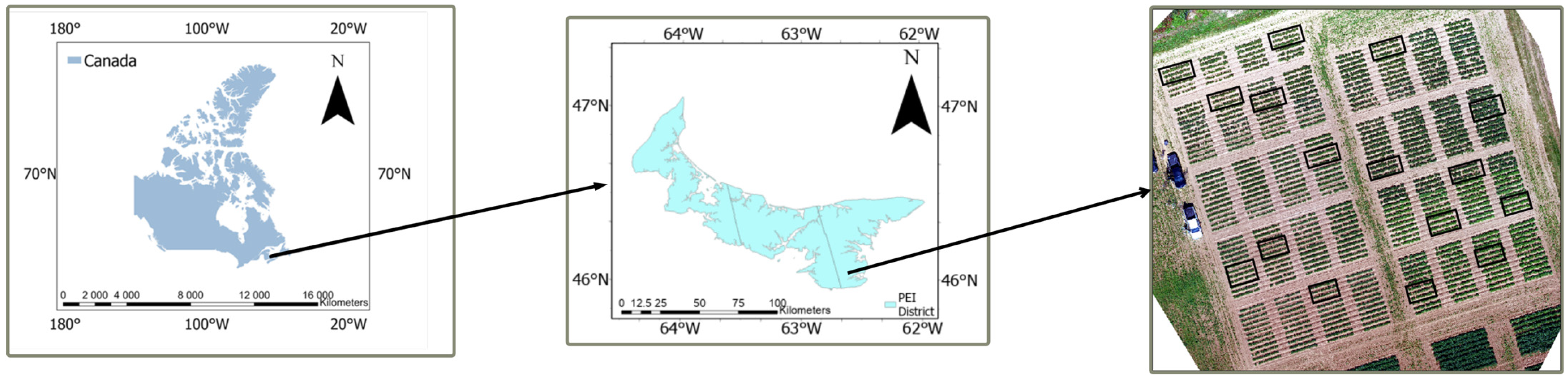
The study area consists of potato plots located in Souris, Prince Edward Island, Canada (Latitude 46.24349° N, Longitude 63.18507° W) (Figure 1). They correspond to plots where fungicides are tested. There were 20 plots treated with fungicides and 16 control plots without fungicide treatment. From each of the 16 plots, three rows were randomly selected for field-based health assessment. The boxes shown in Figure 1 indicate the locations of these selected rows. The potato plants were at varying growth stages, resulting in differences in canopy density. For detailed observations of potato health status, only the control plots were used, as the probability of infected plants is higher in the control plots than in the treated plots. On each control plot, only three randomly selected rows were used for the detailed observations. The infected plants had various PLB disease stages. UAV multispectral imagery was acquired in the summer of 2019 with a DJI Matrice 100 multirotor UAV (designed by A&L, London, ON, Canada) equipped with a MicaSense multispectral camera (MicaSense Inc., Seattle, WA, USA). The camera captured reflectance in five spectral bands, including Blue (475 nm center, 32 nm bandwidth), Green (560 nm center, 27 nm bandwidth), Red (668 nm center, 14 nm bandwidth), Red Edge (717 nm center, 12 nm bandwidth), and Near-Infrared (840 nm center, 57 nm bandwidth). Flight missions were planned and executed using dedicated mission-planning software, ensuring that flight parameters remained consistent throughout the survey. The UAV flights were conducted at an altitude of 100 m above ground level. The resulting imagery achieved a ground sampling distance (GSD) of approximately 1.68 cm. The flights were conducted at noon to maximize the sun’s elevation and minimize the shadow effect. Flight missions were planned in order that the UAV flying 100 m above ground level with 70% overlap between adjacent images. The flights were performed under stable weather conditions, with wind speeds below 20 km/h and partly sunny conditions.

2.2. Methodology

2.2.1. Overview

The acquired UAV multispectral images were orthorectified, mosaicked, and radiometrically corrected using the protocol described in [21], within the Pix4D photogrammetric software (Pix4D SA, Prilly, Switzerland). The radiometric correction was done by comparing the images acquired over the fields to images acquired over a Spectralon panel. The resulting images are reflectance images. Potato plants were detected on the 5-band raw reflectance mosaics using a deep learning Mask R-CNN model (modified from [19]).

To determine the plant health status, two methodologies were tested as follows:

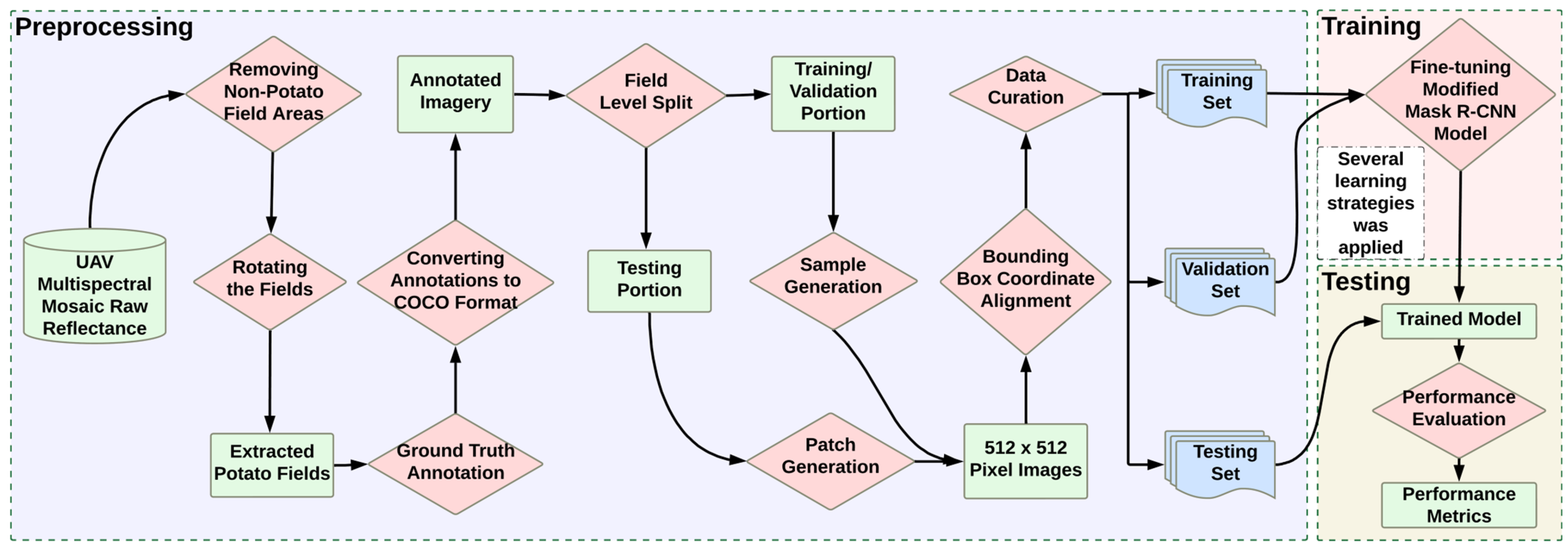
• In the first approach, the same deep learning Mask R-CNN model was applied to the 5-band raw reflectance mosaics (Figure 2).
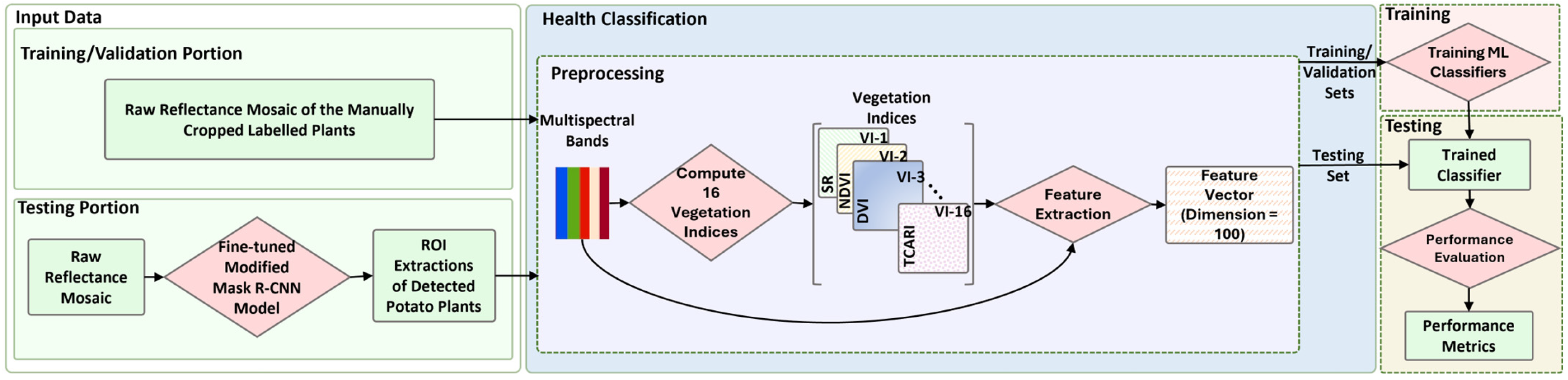
• In the second approach, like in [22], plants detected using the Mask R-CNN algorithm (as in Flow #1) were classified into two categories, healthy and infected, using a machine learning classifier (Figure 3). The classifier was applied to the five-band raw reflectance images and/or 16 associated vegetation indices.

2.2.2. Preprocessing

For both flows, the preprocessing pipeline includes removing non-field areas, rotating fields, ground-truth annotation, and field zoning (Section Removing Non-Field Areas and Rotating the Fields, Section Ground Truth Annotation and Converting to COCO Format and Section Field Zoning). Flow #1 includes additional steps such as training/validation sample generation, testing patch generation, and bounding box alignment with data curation (Section Training and Validation Sample Generation, Section Testing Patch Generation and Section Bounding Box Coordination Alignment and Data Curation). Flow #2 includes additional steps for vegetation index computation and feature extraction (Section Vegetation Index Computation and Section Feature Extraction).

Removing Non-Field Areas and Rotating the Fields

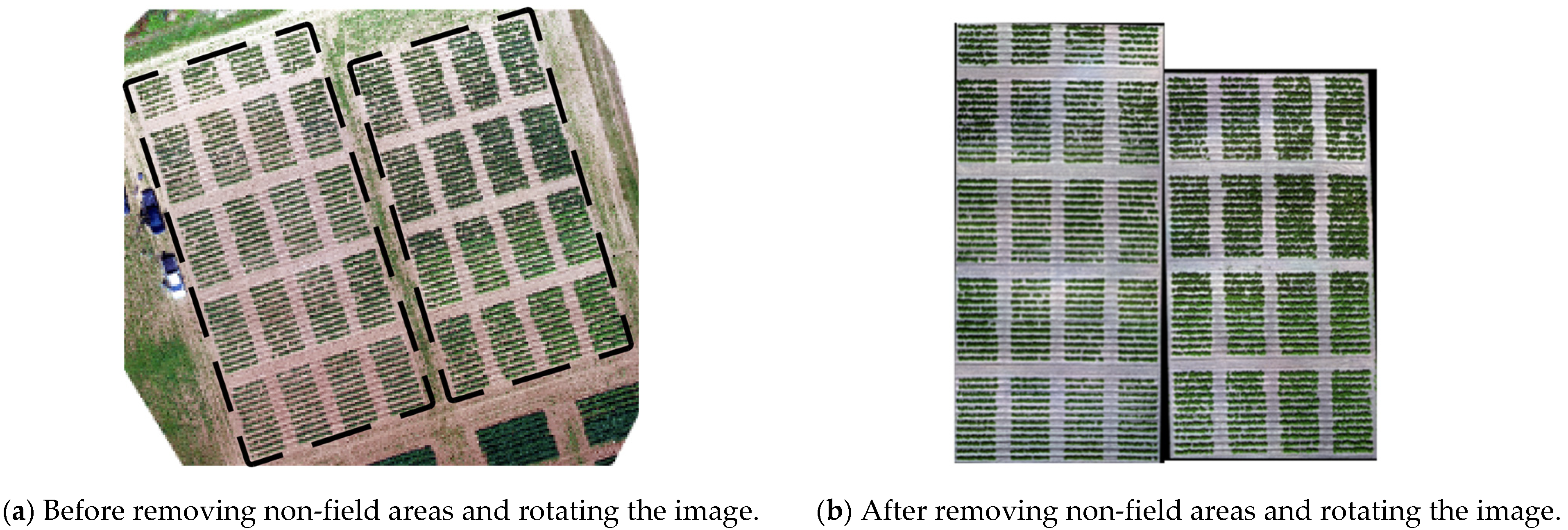
To apply the models solely to the potato plots, non-field areas were removed from the UAV image mosaics, including roads, cars, and several landscape features outside the fields. This removal was done using the “Polygon construction” tool in ArcGIS Pro (version 3.2.0). Due to the orientation of potato field rows in the UAV imagery, a geometric rotation step was applied to align the fields with the image axes. This alignment facilitates more accurate manual annotation by reducing skewed bounding boxes and ensuring consistent object orientation, both of which are particularly important for precise plant-level detection and disease assessment. This rotation was performed using the “Rotate” tool in ArcGIS Pro, and the resulting image was extracted using the “Extract by Mask” tool. Figure 4a shows the potato crop UAV mosaic before removing non-field areas and the rotation, and Figure 4b shows the resulting cropped and rotated imagery.

Ground Truth Annotation and Converting to COCO Format

Among the 36 available plots, 5229 potato plants were annotated and used to test the potato plant detection algorithm. Both the DL and ML algorithms for detecting health status were tested only on the 169 plants surveyed for disease. Ground truth labels were obtained through field observations, where individual potato plants were visually inspected and assigned a health status (healthy or unhealthy). Annotations were performed at the plant level using bounding boxes corresponding to individual plants. These observations were conducted during the growing season at a time close to the UAV image acquisition. The annotations were converted to the COCO format to be compatible with the Mask R-CNN framework. The COCO format standardizes object detection annotations by storing bounding boxes and category labels in a structured JSON file.

Field Zoning

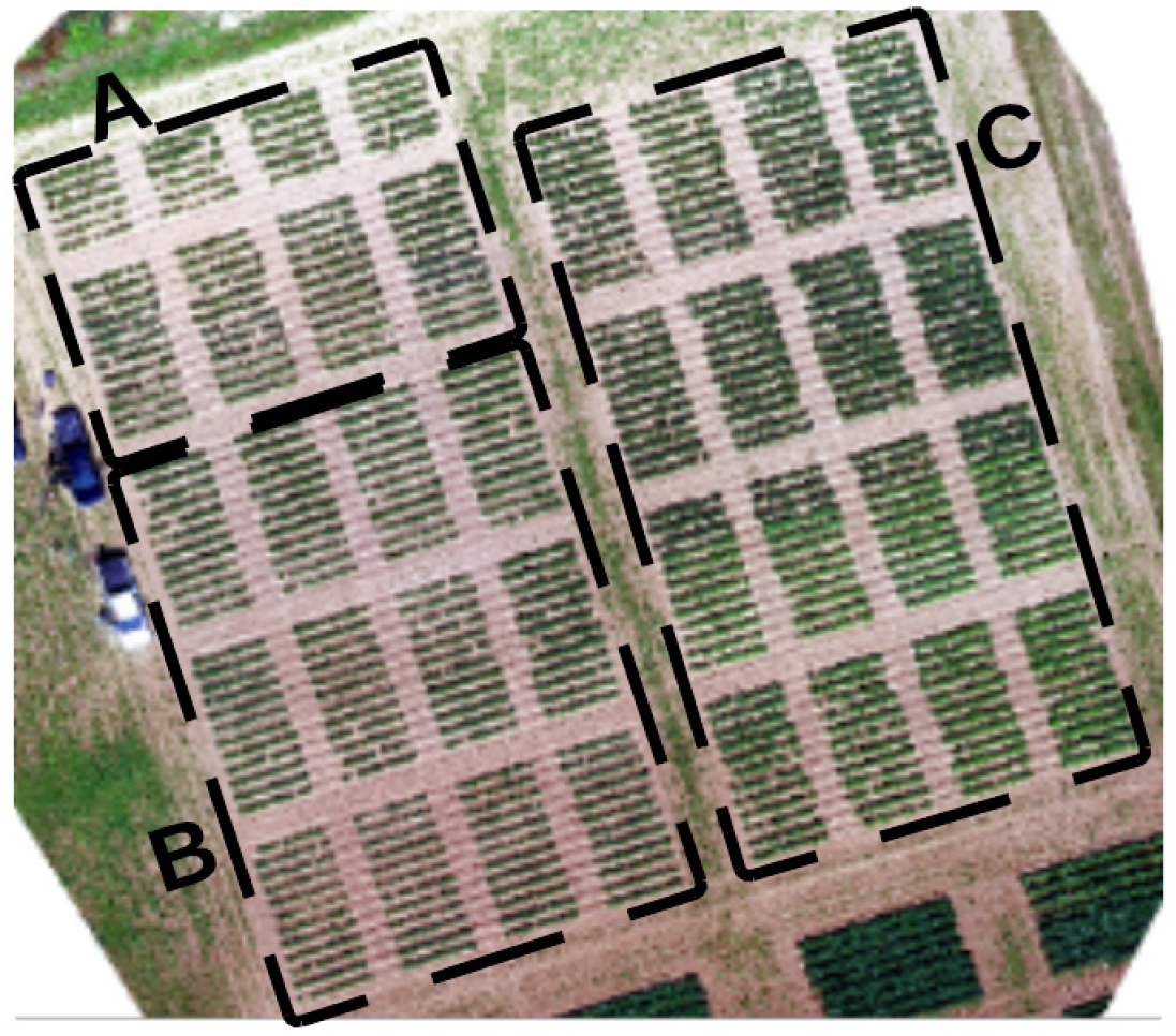
The study area consists of 16 plots that include health-related annotations. Four plots (approximately 25% of the dataset) were grouped into Zone A and used exclusively for testing, while the remaining plots (Zones B and C) were used for training and validation. To prevent data leakage, the entire study area was divided into either the training/validation or the testing zones (Figure 5). This strategy ensures that no plants from the same zone appear in both the training/validation and the testing datasets. It therefore keeps the testing data completely unseen by the model.

Training and Validation Sample Generation

It enhances sample diversity, preserves local spatial context, and improves model robustness, particularly under limited annotation conditions. Following [21], random margin cropping was applied around annotated plants to generate samples. Random margins around potato plant bounding boxes introduce variability in the generated patches and increase data diversity. In each case, a patch size of 512 × 512 pixels was selected. It corresponds to an area of 8.6 m × 8.6 m, given that the total area covered by the UAV image is approximately 0.32 ha. This process was applied to the B and C zones (training/validation) (Figure 5), which have 4320 potato plants, yielding 4320 image patches. Among the 4320 potato plants in these zones, 121 were labelled as healthy or unhealthy and used in the health classification training process.

Testing Patch Generation

During testing, it is essential to evaluate the model on clean and structurally consistent data without augmentation. Therefore, unlike the training/validation sample generation, no random margin cropping was applied to the testing portion. Instead, the testing zone (Zone A on Figure 5) was divided into non-overlapping 512 × 512-pixel patches. These patches were cropped in a grid pattern to cover the test area fully. A total of 12 patches were cropped from the testing field zone, which includes 909 potato plants. Since the split was performed at the field level before patch generation, all test patches are generated from plants unseen during training, ensuring independence between the training and test datasets. Among the 909 potato plants in this section, 48 plants had health-related labels and were used in the health classification testing.

Bounding Box Coordination Alignment and Data Curation

The original annotations were defined in the full field coordinate space. After each cropping operation (both for training/validation sample generation and testing patch extraction), the bounding box coordinates were recalculated to align with the new patch coordinates. Finally, the patches were checked to ensure they were the correct size, that annotations were consistent, and that the data was accurate, to prevent training instability and evaluation errors. This data curation step prepared the training, validation, and test datasets for use by the model.

Vegetation Index Computation

The ML classifier used to classify UAV image samples of potato plants was applied to raw reflectance images and 16 vegetation indices (VIs), as in [22]. These images were calculated using the equations listed in

Table 3. Vegetation indices (VI) were used in the study.

Vegetation Index	Equation	Reference
Simple Ratio	SR = NIR/Red	[23]
Normalized Difference VI	NDVI = (NIR − Red)/(NIR + Red)	[24]
Difference VI	DVI = NIR − Red	[25]
Transformed VI	$\mathrm{TVI}=\sqrt{\mathrm{N}\mathrm{D}\mathrm{V}\mathrm{I}+0.5}$	[26]
Enhanced VI	$\mathrm{EVI} = 2.5 \times$$\left[\right(\mathrm{NIR} - \mathrm{Red})/(1 + \mathrm{NIR} + 6 \times$$\mathrm{Red} - 7.5 \times$ Blue)]	[27]
Soil-Adjusted VI (L is usually equal to 0.5)	SAVI = [(NIR – Red)/(NIR + Red + L)] + (1 + L)	[28]
Optimized Soil-Adjusted VI	OSAVI = (NIR − Red)/(NIR + Red + 0.16)	[29]
Optimized Soil-Adjusted VI 2	OSAVI2 = (1 + 0.16) × (NIR − Red)/(NIR + Red + 0.16)	[30]
Modified Triangular VI	$\mathrm{MTVI} = 1.2 \times$$[1.2 \times$$(\mathrm{NIR} - \mathrm{Green}) - 2.5 \times$ (Red − Green)]	[31]
Green Chlorophyll Index	CIgreen = NIR/Green − 1	[32]
Green NDVI	GNDVI = (NIR − Green)/(NIR + Green)	[33]
Redness Index	RI = (Red − Green)/(Red + Green)	[34]
Red-Edge Chlorophyll Index	CIred-edge = NIR/RedEdge − 1	[32]
Red edge Normalized Difference VI	Red-Edge NDVI = (NIR − RedEdge)/(NIR + RedEdge)	[35]
Transformed Chlorophyll Absorption in Reflectance Index	$\mathrm{TCARI} = 3 \times [$$(\mathrm{RedEdge} - \mathrm{Red}) - 0.2 \times$$(\mathrm{RedEdge} - \mathrm{Green}) \times$ (RedEdge/(NIR + Red)]	[36]
TCARI/OSAVI	TCARI/OSAVI	[37]

. These indices were selected for their proven sensitivity to plant physiological status, chlorophyll content, and the presence of potato late blight [1]. In particular, SR, Cl green, RI, TCARI, TCARI/OSAVI-2 ratio, Cl red-edge, and red-edge NDVI are highly sensitive to the presence of late blight at the leaf and canopy levels [1].

Feature Extraction

To characterize the distribution of spectral responses within each annotated potato plant sample, five statistical descriptors were extracted from the reflectance and vegetation index images: mean, standard deviation, median, 10th percentile (p10), and 90th percentile (p90). The mean represents the average reflectance or vegetation index value within each sample and provides a general measure of overall canopy condition. The standard deviation quantifies the internal variability of spectral responses within the plant region. The median captures the central tendency of spectral values and is less sensitive to extreme values caused by shadows or mixed pixels, making it a more robust indicator of typical plant condition. The p10 emphasizes the lower end of the spectral distribution, highlighting the most stressed portions of the canopy, which are often associated with early disease symptoms. In contrast, the p90 represents the upper end of the distribution and reflects the most vigorous and healthy parts of the plant canopy. These descriptors were aggregated into a feature vector for each plant instance, which was then used as input for traditional machine learning classifiers for predicting plant health status.

2.2.3. Deep Learning Model Fine-Tuning

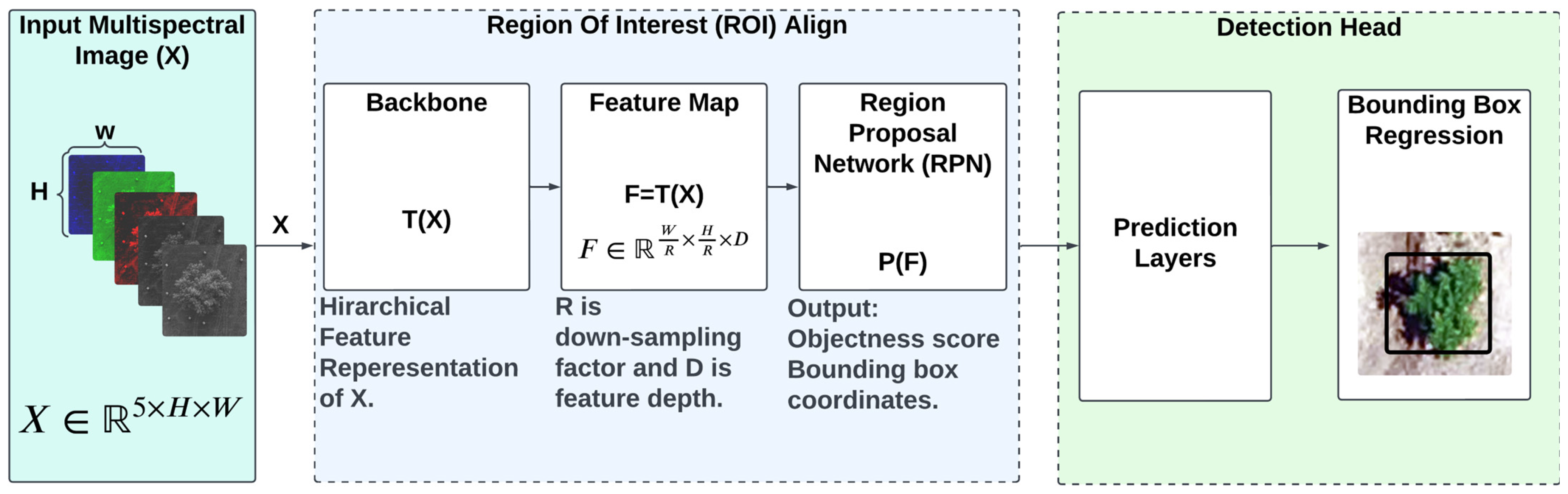
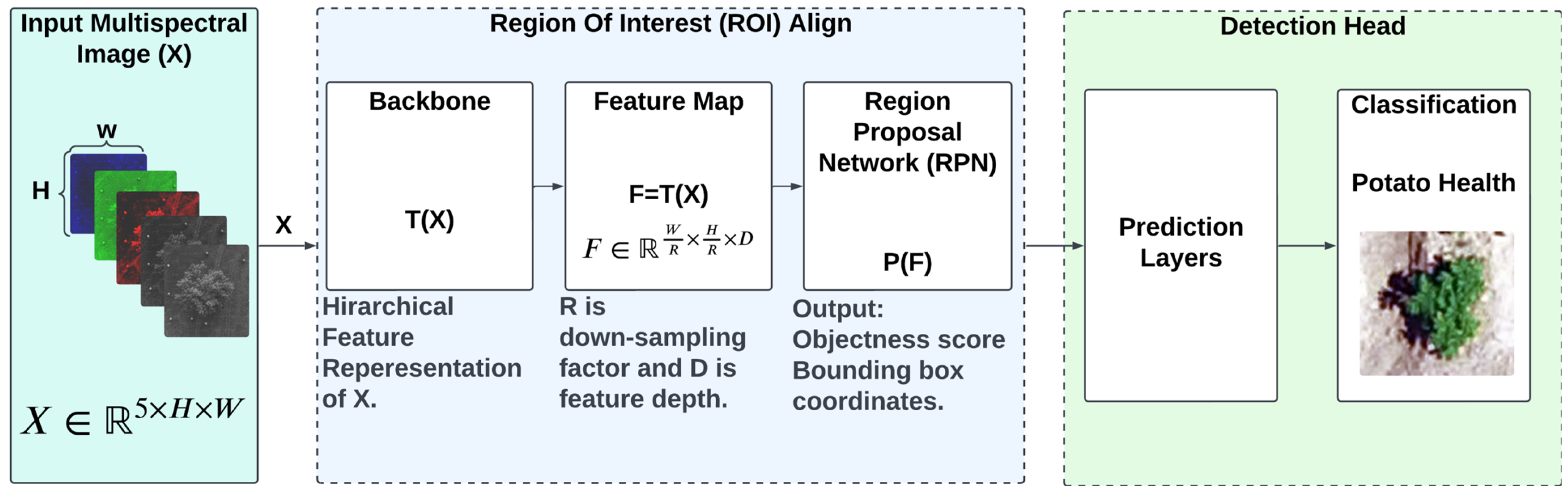
A modified version of the Mask R-CNN model developed by [21] was utilized for potato plant detection and plant health classification (in Flow #1). The model consists of two principal components: a Region of Interest (ROI) alignment module and a detection head that performs bounding-box regression to localize potato plants and classification to assess their health status (Figure 6 and Figure 7). In Mask R-CNN, candidate regions are first generated and then refined through region-wise feature extraction and prediction. This two-stage design was selected to prioritize localization accuracy, which is critical for UAV-based detection of relatively small potato plants. For the plant health detection, disease symptoms may be subtle or spatially localized within the canopy. Although the original Mask R-CNN architecture includes a mask prediction component, it was turned off in the present study. The architecture was instead configured to focus on plant-level detection and health classification. The model was also modified to use 5-band raw reflectance as input (Figure 6 and Figure 7). A modified Mask R-CNN configuration for 5-band raw reflectance has already been shown to outperform other configurations (RGB or 3 principal components) for orchard tree health mapping from multispectral UAV images [21].

For the plant detection step, all 5229 plants were included in the analysis (Figure 6). When Mask R-CNN was used for plant health detection, only the 169 plants with health-related labels were considered (Figure 7). In the proposed framework, potato detection is formulated as a single-object detection task (Figure 6), while plant health classification is treated as a secondary ROI-level classification problem with two supervised classes: Healthy (Class 1) and Unhealthy (Class 2). Additionally, a third category (‘unknown’) is included in the annotations to represent plants without health-related labels (Figure 7).

Mask R-CNN Backbones

For both Mask R-CNN architectures, multiple backbone architectures and training strategies were explored to better address the specific challenges of detecting potato late blight in UAV images. A good backbone selection helps to identify representations that offer robust feature extraction under limited annotation conditions. The first backbone considered here is the ResNeXt-101 [38], due to its superior performance compared to other backbones (ResNet-50, ResNet-101, and Swin Transformer) for orchard tree health mapping using multispectral UAV images [21]. In the present study, ResNeXt-101 was first trained directly on the potato field dataset to establish a baseline performance specific to potato plant detection and health classification. Also, several variants of the DINOv3 vision transformer backbone [20] were tested. DINOv3, introduced by [20], represents a significant advancement in self-supervised learning (SSL) for computer vision. This model scales SSL training to unprecedented levels, utilizing a massive dataset of approximately 1.7 billion images and training models up to 7 billion parameters without any human labels or annotations. DINOv3 introduces a novel regularization technique called Gram anchoring. This method effectively preserves high-quality dense feature maps by anchoring the Gram matrix of patch similarities to an earlier checkpoint (Gram teacher), preventing the collapse of local spatial consistency while maintaining strong global semantic representations. As a result, DINOv3 produces exceptionally robust and versatile visual features that remain clean and semantically meaningful even at high resolutions. These features excel at both global tasks (such as image classification) and especially at dense prediction tasks (semantic segmentation, depth estimation, object detection, keypoint matching, etc.), often outperforming specialized state-of-the-art models, even when the DINOv3 backbone is kept completely frozen (no fine-tuning). The model family includes variants such as Small, Base, and Large that have been tested in this study. In this study, a specialized variant of DINOv3, pretrained on the large-scale dataset most closely aligned with our domain, was also leveraged. Several variants of the original DINOv3 backbones that were tested in this study have varying scales, as well as further adaptations that incorporated contrastive learning, semi-supervised learning, and fine-tuning strategies. All DINOv3 variants were integrated into the modified Mask R-CNN framework and trained using the same preprocessing pipeline, five-band multispectral input, a disabled mask layer, and an evaluation protocol to ensure a fair comparison across configurations. First, the original DINOv3 backbones pretrained on large-scale natural image datasets were evaluated at three different scales: Small, Base, and Large. In addition to the original DINOv3 models, a satellite image-pretrained DINOv3 Large backbone was evaluated. This variant was pretrained on a large-scale satellite imagery dataset, which is spectrally and structurally closer to our UAV imagery than generic natural image datasets.

Table 4. Parameters and GFLOPs of the backbones used in this study.

Backbone	Trainable Parameters (Million)		GFLOPs *
	3-Band	5-Band
Dinov3 Small	21	37.85	112.42
Dinov3 Base	86	102.59	379.31
ResNeXt-101	89	105.64	457.77
Dinov3 Large	300	320.50	1270.52

* GFLOPs = Giga FLOPs = billion floating-point operations (FLOPs) for a single forward pass of one 512 $\times$ 512-pixel image.

summarizes the model complexity of each backbone evaluated in this study. The number of parameters shows the model’s capacity, while GFLOPs (Giga Floating-Point Operations) show the computational complexity required for a single forward pass of a 512 × 512-pixel image. The computational cost increases with the backbone’s scale. The DINOv3 Small model has the fewest parameters for 5-band data (~38 million) and the lowest computational cost. In contrast, the DINOv3 Large backbone is substantially heavier, with approximately 320 million parameters and over 1270 GFLOPs for a 5-band input. The ResNeXt-101 backbone has approximately the same number of parameters as DINOv3 but has a higher computational cost due to its convolutional architecture. In addition, using five spectral bands instead of three increases computational cost across all models, as the network’s first layer processes additional spectral channels.

Class Imbalance Handling

Our field data shows an imbalance between healthy and unhealthy plants. To reduce this bias, a class-weighted Focal Loss was used for the health classification head, as defined in Equation (1).

$${\mathrm{L}}_{\mathrm{health}}={-\mathrm{w}}_{\mathrm{c}}{\left(1-{\mathrm{p}}_{\mathrm{t}}\right)}^{\mathsf{\gamma }}\log \left({\mathrm{p}}_{\mathrm{t}}\right),$$

(1)

where $p_t$ is the predicted probability of the healthy class, $\gamma$ is a focusing parameter, and $w_c$ is the class weight. Class weights were computed based on the inverse class frequencies in the training set using Equation (2).

$${\mathrm{w}}_{\mathrm{c}}={\displaystyle \frac{{\mathrm{N}}_{\mathrm{total}}}{{\mathrm{N}}_{\mathrm{c}}}},$$

(2)

where $N_{\mathrm{total}}$ is the total number of samples and $N_c$ is the number of samples in class c. This ensures that the minority class (unhealthy) has a stronger influence during training. In addition, Focal Loss reduces the contribution of easy and highly confident samples and focuses more on hard examples, which improves robustness under class imbalance.

Transfer Learning Strategy

A transfer learning configuration was evaluated, in which the ResNeXt-101 model that was pretrained on our apple orchard data in our previous study [21] was fine-tuned on the potato dataset. This comparison allowed us to assess the benefit of transferring learned representations from an agricultural application, while also distinguishing it from training the same architecture exclusively on potato field data.

Self-Supervised Learning Strategy

Samples labeled as “unknown” were excluded from supervised health training. These samples were not used to compute health classification loss. This prevents noisy or uncertain labels from negatively affecting the minority class. To still benefit from “unknown” labeled samples, a semi-supervised pseudo-labeling strategy was used. For an unknown ROI sample $x$, the model produces a probability distribution over health classes defined by Equation (3)

$$p\left(y|x\right),$$

(3)

where $x$ is the input ROI feature (cropped region) extracted for one potato instance, $y$ is the class index (1: healthy, 2: unhealthy), $p\left(y|x\right)$ is the probability of the class $y$ given $x$. A pseudo-label $\widehat{y}$ is assigned as the class with the highest predicted probability, calculated by Equation (4). To reduce noise and avoid reinforcing class bias, pseudo-labels are accepted only when the model’s confidence exceeds a chosen threshold of 0.85 in this study.

$$\widehat{y}=\arg \underset{y}{\max }p\left(y|x\right),$$

(4)

where $\widehat{y}$ is the pseudo-label, which is predicted by the model for the unlabeled sample and returns the class index $y$ with the maximum probability.

Progressive Learning Strategy

In training settings, the backbone network was fully frozen, and only the detection head and the health classification head were trained. A progressive training strategy was also applied to test whether it could improve results. During the warm-up phase, the backbone was still frozen. After the warm-up phase, only the last transformer blocks of the Vision Transformer (ViT) backbone were unfrozen, while the remaining backbone layers remained frozen. These unfrozen layers were optimized with a smaller learning rate to ensure controlled adaptation of high-level features. Two configurations of progressive learning were evaluated: progressive learning number 1 and progressive learning number 2. In progressive learning number 1, a 5-epoch warm-up phase was completed, followed by unfreezing the last 3 ViT blocks. In progressive learning number 2, a 3-epoch warm-up phase took place, followed by unfreezing the last 2 ViT blocks. The learning rate for the unfrozen backbone layers was calculated by Equation (5) for both settings.

$$\mathrm{L}{\mathrm{R}}_{\mathrm{ViT}}=\beta \times \mathrm{base}\_\mathrm{lr},$$

(5)

where $L{R}_{\mathit{ViT}}$ is the learning rate applied to the unfrozen ViT blocks, $\mathit{base}\_\mathit{lr}$ is the base learning rate used for the task-specific heads, and $\beta$ is a scaling factor controlling the degree of backbone adaptation, which was set to 0.2 for progressive learning number 1 and 0.1 for progressive learning number 2. In both settings, the reduced backbone learning rate ensures gradual feature adaptation, preventing drastic shifts in representation space. This staged optimization reduces the risk of early feature dominance by the majority class and results in more stable convergence under imbalanced field conditions.

Contrastive Learning Strategy

To improve the consistency of the learned features, a contrastive learning strategy was added at the ROI level. This encourages samples of the same health class to have similar feature representations while increasing the separation between different classes. This representation-level regularization further improves discrimination against minority-class samples. Together, these strategies reduce bias toward the majority class and improve the model’s ability to classify unhealthy plants in imbalanced datasets correctly.

2.2.4. Machine Learning Model Training

Five classical machine learning (ML) classifiers, i.e., Decision Tree (DT) [39], Random Forest (RF) [40], Support Vector Machine (SVM) [41], K-Nearest Neighbors (KNN) [42], and Light Gradient Boosting Machine (LightGBM) [43], were used to classify the health status of potato plants detected by the Mask R-CNN model. They were applied to the original raw reflectance images of the 5 multispectral bands and to 16 associated VIs.

Decision Tree Classifier

It operates by recursively partitioning the input data into smaller subsets based on feature values, forming a tree-like structure. At each node, a splitting criterion such as Gini impurity or entropy is used to select the feature that best separates the data. The process continues until a stopping condition is met, such as reaching a maximum tree depth or a minimum number of samples per node. Decision Trees are easy to interpret and can model nonlinear relationships, but they may overfit if not properly constrained.

Random Forest Classifier

RF is an ensemble learning method that combines multiple decision trees to improve classification accuracy and robustness. Each tree is trained on a bootstrapped subset of the training data, while a random subset of features is considered at each split. The final prediction is obtained through majority voting among all trees. This approach reduces model variance and enhances generalization performance. Random Forest is well-suited for multivariate and nonlinear datasets and has demonstrated strong performance in remote sensing-based classification tasks [13,15,16,18].

Support Vector Machine Classifier

It is a supervised learning algorithm that performs classification by identifying an optimal hyperplane that maximizes the margin between different classes. The margin is the distance from the hyperplane to the closest data points, known as support vectors. For nonlinearly separable data, SVMs employ kernel functions to map input features into a higher-dimensional space, enabling effective separation. SVM is particularly effective in high-dimensional feature spaces.

K-Nearest Neighbors Classifier

KNN is a non-parametric, instance-based learning algorithm used for classification. It assigns a class label to a new sample based on the majority class among its K nearest neighbors in the feature space, determined using a distance metric such as Euclidean distance. KNN does not learn an explicit model during training and is therefore considered a lazy learner. While simple and effective for small datasets, its performance is sensitive to the choice of K and distance metric and may degrade in high-dimensional feature spaces.

Light Gradient Boosting Machine Classifier

LightGBM is a gradient-boosting framework based on decision tree learning. It utilizes a histogram-based approach to discretize continuous features, significantly improving training efficiency and reducing memory consumption. Trees are built sequentially, with each new tree correcting the errors of the previous ensemble. LightGBM incorporates techniques such as feature subsampling, bagging, and regularization to prevent overfitting and improve generalization. Due to its high efficiency and accuracy, LightGBM is well-suited for complex classification problems with large, structured feature sets.

2.2.5. Performance Evaluation

The performance of each model was evaluated in two stages: potato plant detection and health classification. For both stages, the metrics used were precision, recall, and F1-score. Additionally, for the plant detection stage, the mean Intersection over Union (mIoU) was also used, which measures the localization accuracy. Indeed, the spatial overlap between predicted and ground-truth bounding boxes was measured using the Intersection over Union (IoU) metric, defined as the ratio of the area of overlap to the union of the two bounding boxes (Equation (6)). Higher IoU values indicate more accurate localization of potato plant detections.

$$\mathrm{IoU}={\displaystyle \frac{\mathrm{Area} \mathrm{of} \mathrm{Intersection}}{\mathrm{Area} \mathrm{of} \mathrm{Union}}}$$

(6)

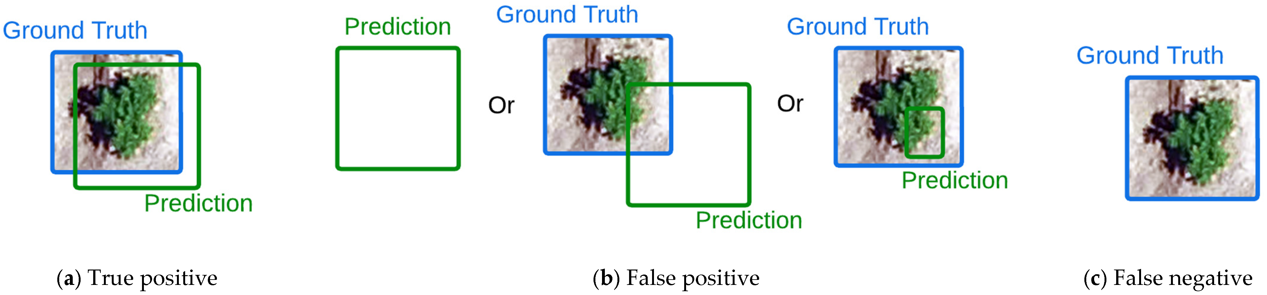
A prediction was considered a true positive (TP) if its bounding box overlapped with a corresponding ground-truth annotation by more than 50%, indicating successful detection and localization of a potato plant. Predictions with an IoU below this threshold or without meaningful overlap with any reference annotation were classified as false positives (FP). Conversely, false negatives (FN) correspond to annotated potato plants that were not detected by the model (Figure 8). The bounding boxes of Figure 8 are enlarged for visualization purposes. In practice, bounding boxes are more tightly fitted around the plant canopy, minimizing the inclusion of background elements such as soil.

Based on these definitions, Precision (Equation (7)) was computed to measure the reliability of positive predictions, while Recall (Equation (8)) quantified the model’s ability to detect all relevant potato plant instances.

$$\mathrm{Precision}={\displaystyle \frac{\mathrm{True} \mathrm{Positive}}{\mathrm{True} \mathrm{Positive}+\mathrm{False} \mathrm{Positive}}}$$

(7)

$$\mathrm{Recall}={\displaystyle \frac{\mathrm{True} \mathrm{Positive}}{\mathrm{True} \mathrm{Positive}+\mathrm{False} \mathrm{Negative}}}$$

(8)

To provide an overall evaluation of the detection performance, the F1-score was calculated as the harmonic mean of Precision and Recall (Equation (9)).

$$\mathrm{F}1-\mathrm{score}={\displaystyle \frac{2\times \mathrm{Precision} \times \mathrm{Recall}}{\mathrm{Precision} +\mathrm{Recall}}}$$

(9)

In this study, for each image in the test set, the precision, recall, and the F1-score were calculated. The reported F1-score values correspond to the average of these per-sample F1-scores (mean of the instance-level F1-score).

3. Results

Table 5. Model performance analysis when the Mask R-CNN model was applied to 5-band multispectral imagery, as a function of the backbone in the case of potato plant detection (total number of samples: 5229; 4320 samples in training and validation dataset, and 909 samples in test set).

Backbone	Precision (%)	Recall (%)	F1-Score (%)	Mean IOU (%)
Finetuning ResNeXt-101 pre-trained model (Transfer Learning)	88.33	81.65	84.20	75.25
ResNeXt101 backbone	87.11	72.38	79.06	72.64
Dinov3 original small backbone	84.74	73.13	78.51	73.40
Dinov3 original large backbone	84.83	73.02	78.48	75.12
Dinov3 original base backbone	85.00	72.81	78.43	73.61
Dinov3 satellite large backbone semi-supervised learning	83.39	72.59	77.62	73.90
Dinov3 satellite large backbone	83.90	71.95	77.46	73.51
Dinov3 satellite large backbone contrastive learning	85.14	70.56	77.17	73.88
Dinov3 satellite large backbone progressive learning 1	78.96	68.31	73.25	69.72
Dinov3 satellite large backbone progressive learning 2	71.82	70.13	70.96	70.07

shows the results for potato plant detection using Mask R-CNN models applied to 5-band multispectral UAV imagery, broken down by backbone. The reported metrics are averages across multiple experiments that yielded very similar results, indicating that the model’s performance is robust and stable. The highest model performance for plant detection across all metrics is achieved by transfer learning from a Mask R-CNN model with a ResNeXt-101 backbone, trained on an apple tree dataset [21]. This process transferred learning from the apple orchard dataset and fine-tuned the model on the potato plant dataset. While training, early stopping was applied, and a fixed random seed was used for data shuffling and weight initialization to ensure consistency.

Table 6. Model performance analysis when the Mask R-CNN model was applied to 5-band multispectral imagery, as a function of the backbone in the case of potato plant health assessment (total number of samples: 169; 121 samples in training and validation dataset, and 48 samples in test set).

Method	Precision (%)	Recall (%)	F1-Score (%)
Dinov3 original small backbone	71.25	70.24	69.05
Dinov3 satellite large backbone, contrastive learning	61.90	62.02	61.89
ResNeXt101 backbone	61.46	61.28	60.88
Dinov3 original large backbone	60.13	59.39	59.38
Dinov3 satellite large backbone progressive training2	58.81	58.89	58.57
Dinov3 satellite large backbone	56.82	56.67	55.49
Dinov3 original base backbone	61.80	58.48	54.17
Finetuning ResNeXt-101 pre-trained model (Transfer Learning)	53.57	53.57	53.33
Dinov3 satellite large backbone semi-supervised learning	52.78	52.56	52.04
Dinov3 satellite large backbone progressive training1	52.68	51.97	50.67

displays the performance metrics for determining the health status of the detected potato plants using the Mask R-CNN model applied to 5-band multispectral UAV imagery, as a function of the backbone. The highest-performing model was achieved with a Mask R-CNN using the Dinov3 original small backbone variant.

It should be noted that the test set used for plant health classification is relatively small (48 samples). Therefore, small differences in performance metrics (e.g., 1–2% in F1-score) may not be statistically significant and should be interpreted with caution.

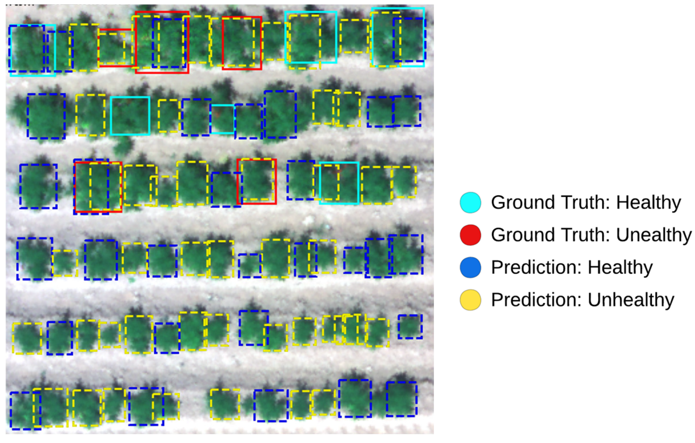
Figure 9 shows an RGB image of the potato plant detection and health classification produced with Mask R-CNN and the Dinov3 small backbone applied to 5-band multispectral UAV imagery. The ground truth is shown with a cyan box for healthy plants and a red box for unhealthy plants. The model-predicted bounding boxes are shown in blue for healthy plants and in yellow for unhealthy plants.

Since the number of plants (169) with a health/unhealth label was small, deep learning models could not perform as well as expected. This is why, as in [22], the detected potato plants were classified into two classes (healthy and infected) using a machine learning classifier. The classifiers were applied to the 5-band raw reflectance images and their 16 associated vegetation indices. The class imbalance between healthy and unhealthy samples was addressed using balanced class weighting during model training.

Table 7. Performance metrics when various machine learning classifiers are applied to the detected potato plants using 5-band raw reflectance images and associated 16 vegetation index images (Total number of samples: 169; 121 samples in training and validation data, and 48 samples in test).

Method	Precision (%)	Recall (%)	F1-Score (%)
Decision Tree	54.55	50.00	51.67
KNN	49.70	42.31	44.52
Random Forest	44.69	38.46	40.77
SVM	44.69	38.46	40.77
LGBM	39.72	34.62	36.81

compares the performance metrics associated with each of the five machine learning classifiers applied to the 5-band raw reflectance images and their 16 associated vegetation indices. The decision tree classifier achieved the best performance metrics.

The various classifiers were also tested only on the 16 vegetation indices, as described in [22]. The results in

Table 8. Performance metrics when various machine learning classifiers were applied to the detected potato plants using the 16 vegetation index images (total number of samples: 169; 121 samples in training and validation data, and 48 samples in test).

Method	Precision (%)	Recall (%)	F1-Score (%)
Decision Tree	72.78	65.38	66.71
Random Forest	57.40	50.00	51.92
SVM	57.40	50.00	51.92
KNN	49.42	46.15	47.56
LGBM	49.42	46.15	47.56

show that overall, all the classifiers performed better than when a combination of 5-band raw reflectance images and associated 16 vegetation indices. Again, the tree classifier achieved the best performance.

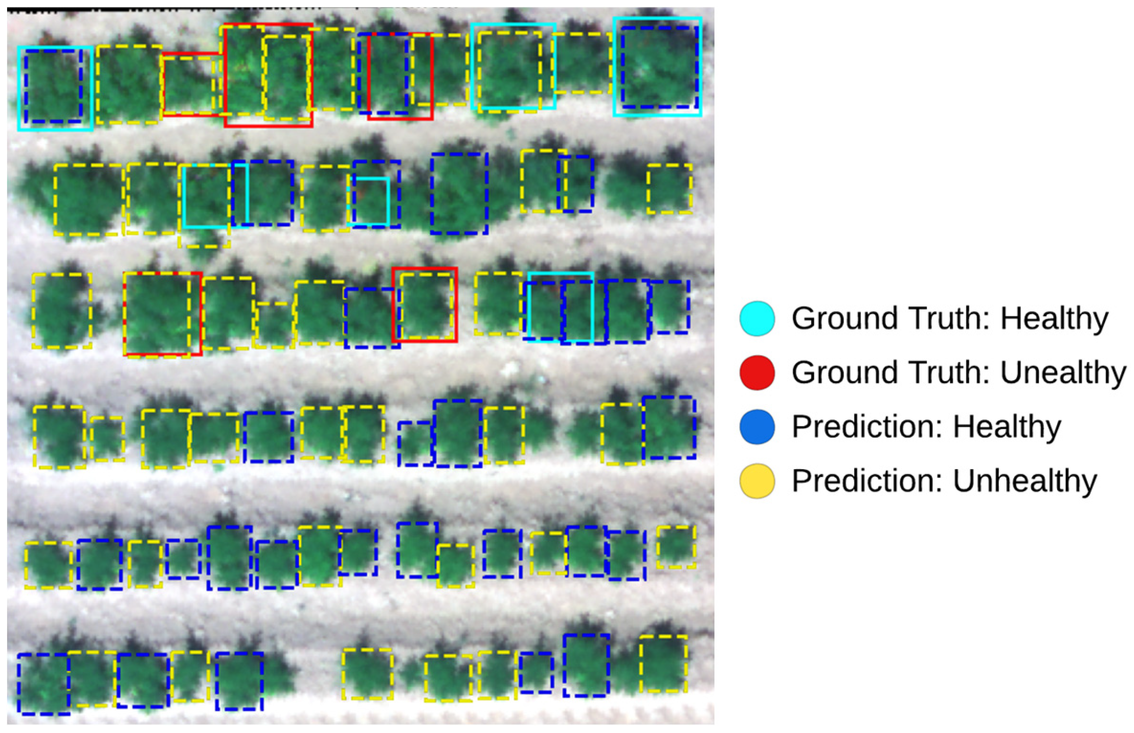
Figure 10 shows an RGB image of potato plant detection and health classification for the best cases: detection using Mask R-CNN with the ResNeXt-101 backbone and transfer learning, and health classification using a decision tree classifier with 16 vegetation indices applied to 5-band multispectral UAV imagery.

For the best case (decision tree classifier applied to the 16 vegetation index images), the top 10 input features were ranked using a feature importance metric estimated via the impurity-based criterion implemented in scikit-learn. In a Decision Tree, each split is selected to maximize the reduction in node impurity. The Gini impurity was adopted as the splitting criterion. For a candidate split, the impurity decrease is defined by Equation (10).

$$\mathsf{\Delta }\mathrm{I}=I(p)-I(R){\displaystyle \frac{R^n}{n}}-I(L){\displaystyle \frac{L^n}{n}},$$

(10)

where I(p) denotes the impurity of the parent node, I(L) and I(R) represent the impurities of the left and right child nodes, and $L^n$ and $R^n$ correspond to the number of samples in the left child, right child, and parent node, respectively.

The importance of each feature is computed as the total weighted impurity reduction contributed by that feature across all splits in the trained tree. The resulting importance values are then normalized so that the sum of all feature importance values equals 1. Features that are not selected for any split receive an importance score of zero, indicating negligible discriminative power within the Decision Tree model. The resulting feature score reflects the relative role of each feature in reducing classification impurity and, consequently, in improving the separability between healthy and unhealthy crop conditions.

Table 9. Ranking of the top 10 input features when the Gini impurity is used as the splitting criterion in a Decision Tree classifier applied to the 16 vegetation index images.

Ranking	Feature	Contribution (%)
1	CIgreen mean	8.95
2	OSAVI2 p10	8.49
3	TCARI median	8.24
4	TCARI/OSAVI2 median	8.04
5	GNDVI median	7.66
6	RedEdge NDVI p10	6.39
7	RI std	5.60
8	CIred-edge std	5.45
9	RedEdge NDVI mean	4.52
10	SR p90	4.41

shows that CIgreen’s mean, OSAVI2’s p10, TCARI’s median, and TCARI/OSAVI2’s median are the most effective in the Decision Tree classifier with a contribution of higher than 8%.

4. Discussion

In this study, Mask R-CNN was first applied to 5-band raw reflectance UAV images for potato plant detection. The best performance was obtained using a ResNeXt-101 backbone with transfer learning, achieving an F1-score of 84.2%. This is slightly lower than the results reported in [17] (88.4%) and [18] (85.9%). For infected plant detection, two approaches were evaluated. In the first, Mask R-CNN was used to jointly detect and classify potato plants in a single stage, with the best F1-score (69.05%) obtained using the DINOv3-S backbone. In the second method, the detected plants were classified by their health status using an ML classifier on 5-band raw reflectance images and associated vegetation index images. Using only the 16 vegetation indices improved classification performance by 15–18% across all metrics compared with using both the 16 index images and the 5-band raw reflectance images together (Table 7 and Table 8). The achieved F-1 score was lower than the one reported by [17] (88.4%) and [18] (85.9%). One possible reason is that classification was performed in our case at the individual plant level, whereas in [17,18], it was conducted at the pixel or zone level. Due to these differences in problem formulation, the reported performance metrics are not directly comparable. It should also be noted that studies on potato late blight detection using UAV multispectral imagery at the plant level remain limited. Therefore, the comparisons of performance results are provided for general context only and should be interpreted with caution. Table 9 shows that the vegetation indices that contributed the most to the classification were CIgreen, CIred-edge, Red-edge NDVI, TCARI, and the TCARI/OSAVI2 ratio. These indices are known to be sensitive to variations in chlorophyll concentration and photosynthetic activity, which are directly influenced by the PLB infection. Potato late blight initially appears on potato leaves as small light- to dark-green water-soaked lesions. As the infection progresses, these lesions expand, dry out, and turn brown to tannish, leading to tissue necrosis. Under favorable humid conditions, white mycelial growth and sporulation develop on the leaf surface, facilitating rapid disease spread. The pathogen primarily infects foliage but can also spread to stems and tubers, resulting in severe damage and yield loss. These observations align with [1], who reported that red-edge-based indices show the greatest spectral differences between healthy and PLB-infected plants, particularly as disease severity increases.

5. Conclusions

In this study, a framework was developed to detect potato plants by applying a Mask R-CNN model to UAV multispectral imagery. The model was pre-trained on another dataset and successfully detected individual potato plants. This shows that a pretrained Mask R-CNN can be used to detect plant health status across different crop types. To determine whether the plant was infected with PLB, two methods were evaluated: a deep learning-based method and a classical machine learning approach applied to vegetation index images. The fact that the model with a DINOv3 small backbone achieved the best F-1 score indicates that lightweight transformer-based backbones perform better with limited data. In contrast, larger models may be more prone to overfitting. Vegetation index-based machine learning models highlight the importance of red-edge and chlorophyll-related features for distinguishing healthy and unhealthy plants. Overall, the study demonstrates the feasibility of using deep learning and machine learning applied UAV images for plant-based monitoring, offering a good alternative to classical pixel- or zone-level classifiers. Our results on plant health determination were based on a limited dataset, and there is a need to test the methodology on a larger dataset. Accessing large datasets on UAV images acquired over PLB-infected plants is challenging because PLB studies can only be conducted in controlled potato fields.

References

1. Fernández, C.I.; Leblon, B.; Haddadi, A.; Wang, K.; Wang, J. Potato Late Blight Detection at the Leaf and Canopy Levels Based in the Red and Red-Edge Spectral Regions. Remote Sens. 2020, 12, 1292. [Google Scholar] [CrossRef] [Scilit]
2. Gold, K.M.; Townsend, P.A.; Chlus, A.; Herrmann, I.; Couture, J.J.; Larson, E.R.; Gevens, A.J. Hyperspectral Measurements Enable Pre-Symptomatic Detection and Differentiation of Contrasting Physiological Effects of Late Blight and Early Blight in Potato. Remote Sens. 2020, 12, 286. [Google Scholar] [CrossRef] [Scilit]
3. Liu, W.; Zhang, Y.; Fan, H.; Zou, Y.; Qin, Y. Detection of Late Blight in Potato Leaves Based on Multi-Feature and SVM Classifier. J. Phys. Conf. Ser. 2020, 1518, 012045. [Google Scholar] [CrossRef] [Scilit]
4. Gao, J.; Westergaard, J.C.; Sundmark, E.H.R.; Bagge, M.; Liljeroth, E.; Alexandersson, E. Automatic Late Blight Lesion Recognition and Severity Quantification Based on Field Imagery of Diverse Potato Genotypes by Deep Learning. Knowl.-Based Syst. 2021, 214, 106723. [Google Scholar] [CrossRef] [Scilit]
5. Mandal, S.N.; Roy, K.; Dan, S.; Mustafi, S.; Dutta, S.; Barman, A.R.; Chakraborty, A. Development of Disease Scoring System for Severity Analysis of Late Blight of Potato Based on Image Processing Approach. Cohesive J. Microbiol. Infect. Dis. 2021, 5, 000601. [Google Scholar] [CrossRef] [Scilit]
6. Qi, C.; Sandroni, M.; Westergaard, J.C.; Sundmark, E.H.R.; Bagge, M.; Alexandersson, E.; Gao, J. In-Field Early Disease Recognition of Potato Late Blight Based on Deep Learning and Proximal Hyperspectral Imaging. arXiv 2021, arXiv:2111.12155. [Google Scholar] [CrossRef] [Scilit]
7. Hou, B.; Hu, Y.; Zhang, P.; Hou, L. Potato Late Blight Severity and Epidemic Period Prediction Based on Vis/NIR Spectroscopy. Agriculture 2022, 12, 897. [Google Scholar] [CrossRef] [Scilit]
8. Garcia Ariza, J.V.; Suarez Baron, M.J.; Junco Orduz, E.A.; González-Sanabria, J.-S. Application of Unsupervised Learning in the Early Detection of Late Blight in Potato Crops Using Image Processing. Inge CuC 2022, 18, 89–100. [Google Scholar] [CrossRef] [Scilit]
9. Suarez Baron, M.J.; Gomez, A.L.; Diaz, J.E.E. Supervised Learning-Based Image Classification for the Detection of Late Blight in Potato Crops. Appl. Sci. 2022, 12, 9371. [Google Scholar] [CrossRef] [Scilit]
10. Feng, J.; Hou, B.; Yu, C.; Yang, H.; Wang, C.; Shi, X.; Hu, Y. Research and Validation of Potato Late Blight Detection Method Based on Deep Learning. Agronomy 2023, 13, 1659. [Google Scholar] [CrossRef] [Scilit]
11. Zarrouk, Y.; Yandouzi, M.; Grari, M.; Bourhaleb, M.; Rahmoune, M.; Hachami, K. Revolutionizing Potato Late Blight Surveillance: UAV-Driven Object Detection Innovations. J. Theor. Appl. Inf. Technol. 2024, 102, 2934–2943. [Google Scholar]
12. Gibson-Poole, S.; Humphris, S.; Toth, I.; Hamilton, A. Identification of the Onset of Disease within a Potato Crop Using a UAV Equipped with Un-Modified and Modified Commercial off-the-Shelf Digital Cameras. Adv. Anim. Biosci. 2017, 8, 812–816. [Google Scholar] [CrossRef] [Scilit]
13. La Parola, C.M. Comparison of Multispectral and Hyperspectral UAV Imagery for Late Blight (Phytophthora infestans) Detection in a Potato (Solanum tuberosum) Field. Master’s Thesis, Universidade de Lisboa, Lisbon, Portugal, 2022. [Google Scholar]
14. Shi, Y.; Han, L.; Kleerekoper, A.; Chang, S.; Hu, T. Novel Cropdocnet Model for Automated Potato Late Blight Disease Detection from Unmanned Aerial Vehicle-Based Hyperspectral Imagery. Remote Sens. 2022, 14, 396. [Google Scholar] [CrossRef] [Scilit]
15. Sun, H.; Song, X.; Guo, W.; Guo, M.; Mao, Y.; Yang, G.; Feng, H.; Zhang, J.; Feng, Z.; Wang, J.; et al. Potato Late Blight Severity Monitoring Based on the Relief-mRmR Algorithm with Dual-Drone Cooperation. Comput. Electron. Agric. 2023, 215, 108438. [Google Scholar] [CrossRef] [Scilit]
16. Loayza, H.; Palacios, S.; Silva, L.; Gastelo, M.; Aponte, M.; Ramírez, D. Aerial Images and Machine Learning Methods to Emulate the Late Blight Severity in Potato Crops; International Potato Center: Lima, Peru, 2023. [Google Scholar]
17. Galvis, J.L.R. Extraction of Morphological and Spectral Features of Potato Plants from High Resolution Multispectral Images. Ph.D. Thesis, Universidad Nacional de Colombia, Bogotá, Colombia, 2021. [Google Scholar]
18. Rodriguez, J.; Lizarazo, I.; Prieto, F.; Angulo-Morales, V. Assessment of Potato Late Blight from UAV-Based Multispectral Imagery. Comput. Electron. Agric. 2021, 184, 106061. [Google Scholar] [CrossRef] [Scilit]
19. He, K.; Gkioxari, G.; Dollár, P.; Girshick, R. Mask r-Cnn. In Proceedings of the IEEE International Conference on Computer Vision, Venice, Italy, 22–29 October 2017; pp. 2961–2969. [Google Scholar]
20. Siméoni, O.; Vo, H.V.; Seitzer, M.; Baldassarre, F.; Oquab, M.; Jose, C.; Khalidov, V.; Szafraniec, M.; Yi, S.; Ramamonjisoa, M.; et al. DINOv3 2025. arXiv 2025, arXiv:2508.10104. [Google Scholar]
21. Kaviani, M.; Leblon, B.; Akilan, T.; Amishev, D.; LaRocque, A.; Haddadi, A. Tree Health Assessment Using Mask R-CNN on UAV Multispectral Imagery over Apple Orchards. Remote Sens. 2025, 17, 3369. [Google Scholar] [CrossRef] [Scilit]
22. Jemaa, H.; Bouachir, W.; Leblon, B.; LaRocque, A.; Haddadi, A.; Bouguila, N. UAV-Based Computer Vision System for Orchard Apple Tree Detection and Health Assessment. Remote Sens. 2023, 15, 3558. [Google Scholar] [CrossRef] [Scilit]
23. Jordan, C.F. Derivation of Leaf-Area Index from Quality of Light on the Forest Floor. Ecology 1969, 50, 663–666. [Google Scholar] [CrossRef] [Scilit]
24. Rouse, W. Monitoring Vegetation System in the Great Plain with ERTS. In Proceedings of the 3rd ERTS Symposium, Washington, DC, USA, 10–14 December 1973; NASA: Washington, DC, USA, 1973; Volume 1, pp. 309–317. [Google Scholar]
25. Tucker, C.J. Red and Photographic Infrared Linear Combinations for Monitoring Vegetation. Remote Sens. Environ. 1979, 8, 127–150. [Google Scholar] [CrossRef] [Scilit]
26. Perry, C.R., Jr.; Lautenschlager, L.F. Functional Equivalence of Spectral Vegetation Indices. Remote Sens. Environ. 1984, 14, 169–182. [Google Scholar] [CrossRef] [Scilit]
27. Matsushita, B.; Yang, W.; Chen, J.; Onda, Y.; Qiu, G. Sensitivity of the Enhanced Vegetation Index (EVI) and Normalized Difference Vegetation Index (NDVI) to Topographic Effects: A Case Study in High-Density Cypress Forest. Sensors 2007, 7, 2636–2651. [Google Scholar] [CrossRef] [Scilit] [PubMed]
28. Huete, A.R. A Soil-Adjusted Vegetation Index (SAVI). Remote Sens. Environ. 1988, 25, 295–309. [Google Scholar] [CrossRef] [Scilit]
29. Rondeaux, G.; Steven, M.; Baret, F. Optimization of Soil-Adjusted Vegetation Indices. Remote Sens. Environ. 1996, 55, 95–107. [Google Scholar] [CrossRef] [Scilit]
30. Zhu, H.; Chu, B.; Zhang, C.; Liu, F.; Jiang, L.; He, Y. Hyperspectral Imaging for Presymptomatic Detection of Tobacco Disease with Successive Projections Algorithm and Machine-Learning Classifiers. Sci. Rep. 2017, 7, 4125. [Google Scholar] [CrossRef] [Scilit]
31. Haboudane, D.; Miller, J.R.; Pattey, E.; Zarco-Tejada, P.J.; Strachan, I.B. Hyperspectral Vegetation Indices and Novel Algorithms for Predicting Green LAI of Crop Canopies: Modeling and Validation in the Context of Precision Agriculture. Remote Sens. Environ. 2004, 90, 337–352. [Google Scholar] [CrossRef] [Scilit]
32. Gitelson, A.A.; Viña, A.; Ciganda, V.; Rundquist, D.C.; Arkebauer, T.J. Remote Estimation of Canopy Chlorophyll Content in Crops. Geophys. Res. Lett. 2005, 32, L08403. [Google Scholar] [CrossRef] [Scilit]
33. Mirik, M.; Ansley, R.J.; Michels, G.J.; Elliott, N.C. Spectral Vegetation Indices Selected for Quantifying Russian Wheat Aphid (Diuraphis noxia) Feeding Damage in Wheat (Triticum aestivum L.). Precis. Agric. 2012, 13, 501–516. [Google Scholar] [CrossRef] [Scilit]
34. Escadafal, R.; Huete, A. Etude Des Propriétés Spectrales Des Sols Arides Appliquée à l’amélioration Des Indices de Végétation Obtenus Par Télédétection. Comptes Rendus L’académie Sci. Série 2 Mécanique Phys. Chim. Sci. L’univers Sci. Terre 1991, 312, 1385–1391. [Google Scholar]
35. Sharma, L.K.; Bu, H.; Denton, A.; Franzen, D.W. Active-Optical Sensors Using Red NDVI Compared to Red Edge NDVI for Prediction of Corn Grain Yield in North Dakota, USA. Sensors 2015, 15, 27832–27853. [Google Scholar] [CrossRef] [Scilit]
36. Devadas, R.; Lamb, D.W.; Simpfendorfer, S.; Backhouse, D. Evaluating Ten Spectral Vegetation Indices for Identifying Rust Infection in Individual Wheat Leaves. Precis. Agric. 2009, 10, 459–470. [Google Scholar] [CrossRef] [Scilit]
37. Wu, C.; Niu, Z.; Tang, Q.; Huang, W. Estimating Chlorophyll Content from Hyperspectral Vegetation Indices: Modeling and Validation. Agric. For. Meteorol. 2008, 148, 1230–1241. [Google Scholar] [CrossRef] [Scilit]
38. Xie, S.; Girshick, R.; Dollár, P.; Tu, Z.; He, K. Aggregated Residual Transformations for Deep Neural Networks. In Proceedings of the IEEE Conference on Computer Vision and Pattern Recognition, Honolulu, HI, USA, 21–26 July 2017; pp. 1492–1500. [Google Scholar]
39. Loh, W. Classification and Regression Trees. WIREs Data Min. Knowl. Discov. 2011, 1, 14–23. [Google Scholar] [CrossRef] [Scilit]
40. Breiman, L. Random Forests. Mach. Learn. 2001, 45, 5–32. [Google Scholar] [CrossRef] [Scilit]
41. Cortes, C.; Vapnik, V. Support-Vector Networks. Mach. Learn. 1995, 20, 273–297. [Google Scholar] [CrossRef] [Scilit]
42. Steinbach, M.; Tan, P.-N. kNN: K-Nearest Neighbors. In The Top Ten Algorithms in Data Mining; Chapman and Hall: Boca Raton, FL, USA; CRC: Boca Raton, FL, USA, 2009; pp. 165–176. [Google Scholar]
43. Ke, G.; Meng, Q.; Finley, T.; Wang, T.; Chen, W.; Ma, W.; Ye, Q.; Liu, T.-Y. Lightgbm: A Highly Efficient Gradient Boosting Decision Tree. In Proceedings of the 31st Conference on Neural Information Processing Systems (NIPS 2017), Long Beach, CA, USA, 4–9 December 2017. [Google Scholar]
Figure 1. Location of the study area and experimental setting. The black boxes on the field indicate the 16 control plots, with 3 randomly selected rows used for detailed plant health observations.
Remotesensing 18 01292 g001
Figure 2. Flowchart presenting the methodology of Flow #1 for potato plant detection and health classification on the UAV imagery based on a Mask R-CNN deep learning algorithm. Processes are shown with red diamonds, and outputs are shown with green rectangles.
Remotesensing 18 01292 g002
Figure 3. Flowchart of the machine learning methodology for Flow #2 used to classify plants based on their health status. The plants were detected using the Mask R-CNN model of Flow #1. Processes are shown with red diamonds, and outputs are shown with green rectangles.
Remotesensing 18 01292 g003
Figure 4. RGB composite of the UAV mosaics.
Remotesensing 18 01292 g004
Figure 5. Field zoning of the study area as a function of the dataset types. Zone A is assigned to the testing set. Zones B and C are assigned to the training/validation sets.
Remotesensing 18 01292 g005
Figure 6. Modified Mask R-CNN architecture used in this study for potato plant detection.
Remotesensing 18 01292 g006
Figure 7. Modified Mask R-CNN architecture used in this study for potato health assessment.
Remotesensing 18 01292 g007
Figure 8. (a) True positive: the predicted bounding box and the ground truth overlap significantly (with IoU > 50%). (b) False positive: the predicted bounding box and the ground truth bounding box either do not overlap or overlap minimally (IoU < 50%). (c) False negative: the ground truth bounding box is not detected (adapted from [21]).
Remotesensing 18 01292 g008
Figure 9. RGB image showing the potato plant detection and health classification when the Mask R-CNN with Dinov3 small backbone was applied to 5-band multispectral UAV imagery.
Remotesensing 18 01292 g009
Figure 10. RGB image showing the potato plant detection using the Mask R-CNN with ResNeXt-101 backbone (transfer learning technique) and health classification using a decision tree with 16 vegetation indices, applied to 5-band multispectral UAV imagery.
Remotesensing 18 01292 g010