Synthetic Aperture Imaging with ⊤-, $+$-, or $\times$-Shaped Arrays: Cartesian or Hexagonal Sampling?

Highlights

What are the main findings?

• Key parameters of an antenna array devoted to imaging radiometry must be established in a specific order: first the parameters setting the shape and the extent of the alias-free field-of-view, then those driving the spatial resolution, and finally those governing the radiometric sensitivity.
• This study shows how it is possible to perform aperture synthesis on hexagonal sampling grids with antenna arrays whose geometry naturally leads to Cartesian sampling grids, with fewer, but wider, elementary antennas and without degrading imaging performance.

What are the implications of the main findings?

• For these arrays operating aperture synthesis on Cartesian sampling grids but suffering from very, even too close elementary antennas, the short spacing can be increased by slightly changing the location of the antennas in order to perform aperture synthesis on hexagonal grids, without modifying the shape, the dimensions, or the performance of the imaging radiometer.
• The FRESCH project was initially designed for performing aperture synthesis over Cartesian grids with a four-arm array fed with 171 small antennas and a short spacing set to $0.71\lambda$. Thanks to this study, it is possible to enlarge this short spacing up to $0.82\lambda$ and to carry out aperture synthesis over hexagonal grids with 167 wider antennas distributed over the same four arms and with the same imaging performance.

Abstract

The key performance of microwave imaging radiometers by aperture synthesis is governed by spatial resolution, radiometric sensitivity, and the extent of the synthesized field of view that is free from any aliasing artifact. Accordingly, this work is concerned with the choice of key parameters of an antenna array, such as its geometrical shape and the number of elementary antennas as well as their spacing, in order to meet the required scientific specifications and satisfy the necessary engineering constraints. This study is illustrated with two examples: the $+$-shaped array selected for the Fine Resolution Explorer for Salinity, Carbon, and Hydrology (FRESCH) and a ⊤-shaped array proposed for use onboard a High-Altitude Pseudo-Satellite (HAPS), being two high-resolution microwave imaging radiometers by aperture synthesis. Both cases show how it is possible to perform aperture synthesis on hexagonal sampling grids with antenna arrays whose geometry naturally leads to Cartesian sampling grids, with fewer elementary antennas and without degrading imaging performance while also solving computational issues.

1. Introduction

When dealing with microwave imaging [1] and particularly with microwave imaging by aperture synthesis [2], the key performance of an imaging radiometer is governed by a few figures of merit. Spatial resolution and radiometric sensitivity are the most important indicators [3], together with the extent and the shape of the synthesized field of view that is free from any aliasing artifact [4]. This article sheds light on the choice of key instrumental parameters required to meet the specifications established by scientists as well as the constraints imposed by engineers [5]. Among the many particularities of any microwave imaging radiometer, the geometrical shape and the orientation of the antenna array [6], along with the number of elementary antennas and their spacing, are the most important ones. However, without making an exhaustive list, it is also necessary to mention the integration time, the directivity and efficiency of each elementary antenna, and the bandwidth and noise factor of every receiver. As aperture synthesis [7] is an indirect imaging technique that requires the aid of a computer to retrieve brightness temperature maps from interferometric measurements [8], elements of data processing like the apodization window [9] should also be considered.

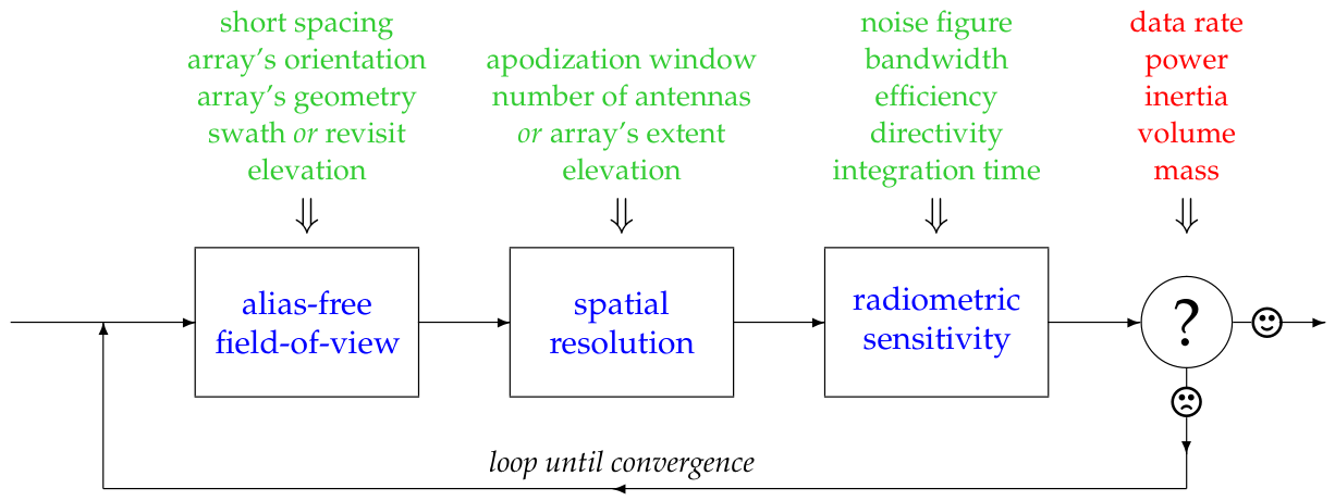
The key instrumental parameters must be established in a specific order while taking into account the associated constraints imposed by scientists in terms of performances and by engineers in terms of error budgets. Indeed, in the words of [10] “Trade-offs need to be considered and priorities must be set in order to realize strategic decisions.” The settings thus obtained can be adjusted within an iterative process during which they will be revisited [11], but always in the same order: first the instrumental parameters that define the shape and the extent of the alias-free field-of-view, then those driving the spatial resolution, and finally those governing the radiometric sensitivity, as illustrated by the block diagram in Figure 1. The number of elementary antennas of the array is a very representative example of the order in which these parameters have to be established. Indeed, as soon as the shortest spacing between the antennas has been chosen for setting an appropriate alias-free field of view, the spatial resolution being governed by the extent of the array is then determined, driven by the number of elementary antennas. However, radiometric sensitivity is also driven by the number of elementary antennas because it is governed by the total collecting area of the array. If spatial resolution requires a larger array, the number of antennas has to be increased, but that will also augment the total collecting area and therefore affect the radiometric sensitivity. Conversely, if the collecting area has to be increased for improving the radiometric sensitivity, the number of antennas can be augmented without affecting the spatial resolution (because antennas can be added without changing the dimensions of the array). This is why, when setting the number of elementary antennas, spatial resolution is taken into account before radiometric sensitivity is considered, in order to avoid the “conflicting situation” pointed out in [12].

Owing to their roles in synthesis imaging, the observing equation of imaging radiometers by aperture synthesis is recalled in Section 2, together with the regularized approach for inverting the interferometric measurements in order to estimate the brightness temperature distribution of the scene observed by an array of elementary antennas. The next three sections are developed in the order shown in Figure 1. The impact of the geometry and the orientation of the antenna array, as well as that of the spacing between the elementary antennas, on the extent and on the shape of the alias-free field of view are addressed in Section 3. Section 4 is devoted to the extent of the array, or in other words the number of elementary antennas populating the array, in order to meet the specific requirements in terms of spatial resolution at ground level. The apodization window introduced in the first section is, of course, taken into account. Then, the instrumental parameters already set are used for estimating the integration time, and, together with others, their impact on the radiometric sensitivity is investigated in Section 5. Finally, the results thus obtained are discussed and interpreted in Section 6 together with limitations.

Figure 1. Block diagram of the iterative process that aims at setting instrumental parameters (green) of a synthetic aperture imaging radiometer in order to satisfy the constraints established by scientists on its performance (blue), while remaining within error budgets (red) imposed by engineers.

Figure 1. Block diagram of the iterative process that aims at setting instrumental parameters (green) of a synthetic aperture imaging radiometer in order to satisfy the constraints established by scientists on its performance (blue), while remaining within error budgets (red) imposed by engineers.

In every section addressing each of the three steps of the iterative process shown in Figure 1, this study is illustrated with the aid of numerical simulations conducted with the Matlab toolbox TRIMARAN [13] for two specific cases: the original $\times$-shaped array, as well as an alternative $+$-shaped one, selected for the Fine Resolution Explorer for Salinity, Carbon and Hydrology (FRESCH) mission, and a ⊤-shaped array proposed for use onboard a High-Altitude Pseudo-Satellite (HAPS), two examples of high-resolution microwave imaging radiometers by aperture synthesis. In both cases, two strategies of populating these arrays with elementary antennas regularly spaced along each arm are compared. The first having the same spacing along every arm of the array, leads to brightness temperature maps sampled over Cartesian grids. The second, without changing the geometry of these arrays nor the extent of their arms, but with two different spacings along perpendicular arms, allows the brightness temperature distributions to be retrieved over hexagonal sampling grids. It is well-known that these two sampling grids are the only possible solutions for regularly paved 2D Euclidean spaces [14]. Apart from the simple difference between the locations of the brightness temperature samples, which does not raise any problem (chap. 7 in [15]), the polygonal shape of the synthesized field-of-view (square vs. hexagon) as well as the geometry governing the field aliasing (4 aliases vs. 6) are highly affected by this choice. The pros and cons of each approach are discussed, and an answer to the question formulated in the title of this article is finally given.

Before going into the details on how to select an optimal configuration for the antenna array of a synthetic aperture imaging radiometer, a few words must be said about the two cases that serve as a common thread throughout this study.

• The SMOS (Soil Moisture & Ocean Salinity) [16] mission was launched in 2009 by ESA and CNES with the single payload MIRAS (Microwave Imaging Radiometer by Aperture Synthesis) [17] onboard. For more than 16 years it has provided accurate radiometric brightness temperature maps for retrieving near-surface soil moisture (SM) [18], even under dense vegetation canopies, as well as ocean salinity (OS) [19], even with strong wind conditions like under hurricanes and typhoons. FRESCH [20] is a proposed high-resolution follow-on mission [21] to maintain the continuity of operational L-band measurements [22]. It is a true multi-polarization and multi-incidence angle imaging radiometer by aperture synthesis with elementary antennas distributed along a cross with four orthogonal arms, each ∼9 m long. The target ground resolution is about 10 km without apodization (15 km with apodization), and the objective for the radiometric sensitivity is about 1.5 K over the ocean [23]. Keeping in mind that a comparison is not as easy as it seems, because the devil is sometimes in the details, and, although, this is not the objective of this study, these values can be compared to the main features of comparable L-band missions SMOS, AQUARIUS, and SMAP (Table 1 in [24]) as well as to those of the future multi-channel CIMR (Table 1 in [25]). FRESCH was submitted to the ESA Earth Explorer 12 program [26] and was evaluated as a “commended mission.” As a consequence, it is currently running an ESA pre-phase 0 study to consolidate the compliance to scientific requirements and to strengthen the technical solutions before being resubmitted to the Earth Explorer 13 program in due time.
• The Monash project proposes a state-of-the-art near-space observation concept for natural disaster risk prediction and monitoring using continuous L-band passive microwave sensing. By leveraging High-Altitude Pseudo-Satellites (HAPS) platforms operating in the stratosphere [27], at a higher altitude than FAA-regulated Class A airspace [28] that ends at flight level FL600 (60,000 feet, i.e., 18 km), the system enables persistent, round-the-clock regional observations with spatial resolution significantly finer than that achievable from conventional satellite missions. The reduced observation altitude enhances spatial detail while preserving wide-area coverage. Operating in the protected L-band, the proposed interferometric radiometer exploits the strong sensitivity of microwave brightness temperature to surface dielectric properties, making it particularly suitable for soil moisture monitoring [29] and related hydrological applications [30]. Through aperture synthesis techniques, the instrument aims to generate high-resolution brightness temperature maps [31] to support improved monitoring of droughts, floods, fires, and landslides. The research studies conducted at Monash aim at establishing the first near-space passive microwave capability dedicated to natural disaster monitoring. By combining scientific advancement with operational flexibility, the Monash HAPS initiative bridges the gap between satellite-scale observation and localized, high-resolution disaster response.

Finally, it is important to keep in mind that this study does not intend to provide the definitive mission parameters of FRESH, nor those of HAPS. Only one iteration of the optimizing process shown in Figure 1 is reported here. It is obvious that these parameters will mature, as well as the performances of the corresponding instruments. The idea is here to provide a framework for making them evolve all together towards an expected direction.

2. Synthesis Imaging

The interferometric measurements provided by an aperture synthesis radiometer are obtained by cross-correlating the signals collected by pairs of non-directive elementary antennas pointing in the same direction and sharing the same field of view [32], yielding samples of the complex degree of coherence V (u) for spatial frequencies u (chap. 10 in [33]). The relationship between these so-called complex visibilities and the brightness temperature of the scene under observation is the well-known van Cittert–Zernike theorem that was first established by Pieter Hendrik van Cittert in 1934 [34] and later more generally by Frits Zernike in 1938 [35]. It has been recently revisited [36] in order to take into account the mutual coupling of close elementary antennas [37,38]. Regardless of polarimetric considerations [39], for every pair of elementary antennas ${\mathcal{A}}_p$ and ${\mathcal{A}}_q$, the complex visibility $V_{pq}\equiv V\left({\mathbf{u}}_{pq}\right)$ is given by:

$${\displaystyle V_{pq}=\int \underset{\parallel \mathsf{\xi }\parallel \le 1}{\int }\frac{{\mathcal{F}}_p\left(\mathsf{\xi }\right)}{\sqrt{{\mathrm{\Omega }}_p}}\frac{{\mathcal{F}}_q^{\ast }\left(\mathsf{\xi }\right)}{\sqrt{{\mathrm{\Omega }}_q}}\tilde{r}(-\frac{{\mathbf{b}}_{pq}·\mathsf{\xi }}{c})(T_b\left(\mathsf{\xi }\right)-T_{rec}){\mathrm{e}}^{{\displaystyle {\displaystyle -2j\pi \frac{{\mathbf{b}}_{pq}·\mathsf{\xi }}{\lambda }}}}\frac{\mathrm{d}\mathsf{\xi }}{\sqrt{1-{\parallel \xi \mathit{\parallel }}^2}},}$$

(1)

where ${\mathbf{b}}_{pq}={\mathbf{r}}_q-{\mathbf{r}}_p$ is the baseline vector from ${\mathcal{A}}_p$ to ${\mathcal{A}}_q$ (${\mathbf{r}}_p$ and ${\mathbf{r}}_q$ are the location vectors of the two elementary antennas with respect to the phase center of the array). The components ${\xi }_1=sin\theta cos\varphi$ and ${\xi }_2=sin\theta sin\varphi$ of the angular position variable $\mathsf{\xi }$ are direction cosines ($\theta$ and $\varphi$ are the traditional spherical coordinates) in the reference frame of the instrument, ${\mathcal{F}}_p\left(\mathsf{\xi }\right)$ and ${\mathcal{F}}_q\left(\mathsf{\xi }\right)$ are the field patterns of the two elementary antennas ${\mathcal{A}}_p$ and ${\mathcal{A}}_q$ with equivalent solid angles ${\mathrm{\Omega }}_p$ and ${\mathrm{\Omega }}_q$, $T_b\left(\mathsf{\xi }\right)$ is the brightness temperature distribution of the observed scene, $T_{rec}$ is the physical temperature of the receivers (assumed to be the same for all the receivers), $\tilde{r}\left(t_{pq}\right)$ is the so-called fringe-washing function [40] which accounts for spatial decorrelation effects for the time delay $t_{pq}=-{\mathbf{b}}_{pq}·\mathsf{\xi }/c$, and $\lambda =c/f$ is the central wavelength of the observation.

Retrieving the unknown brightness temperature distribution $T_b\left(\mathsf{\xi }\right)$ with the aid of a computer from a finite number of complex visibilities $V_{pq}$ goes through a preliminary step for the discretization of the double integral in the modeling Equation (1) over an appropriate sampling grid in the domain of the direction cosines $\mathsf{\xi }$. The relationship between a set of complex visibilities V and the brightness temperature $T_b$ of the corresponding pixels can therefore be written in a very simple linear algebraic form:

$$V=\mathbf{G}T,$$

(2)

where G is the linear modeling matrix of the instrument derived from (1). The inverse problem aims at retrieving $T=T_b$ (the constant $T_{rec}$ is canceled out from the visibilities with the aid of the response to a flat target [41], whatever the method used for the inversion [42]). This inverse problem is ill-posed [43] and so has to be regularized in order to provide a unique and stable solution $\tilde{T}$ for T. Among the regularization methods found in the literature [44], the minimum-norm solution is widely used in imaging radiometry by aperture synthesis [45] such that:

$$\tilde{T}=arg\underset{T}{min}{\parallel T\parallel }^2\mathrm{s.t.}\mathbf{G}T=V.$$

(3)

This map is obtained through computation of the Moore–Penrose [46,47] pseudo-inverse ${\mathbf{G}}^{+}$ of G:

$$\tilde{T}={\mathbf{G}}^{+}V.$$

(4)

Referring back to the samples $V_{pq}\equiv V\left({\mathbf{u}}_{pq}\right)$ of the complex degree of coherence $V\left(\mathbf{u}\right)$, the spatial frequencies ${\mathbf{u}}_{pq}\equiv {\mathbf{b}}_{pq}/\lambda$ sampled by an aperture synthesis radiometer are confined to a bounded region of the Fourier domain, the so-called experimental frequency coverage, as a consequence of the finite number of elementary antennas. The support of the Fourier transform of $\tilde{T}$ is therefore limited to this region. In order to filter out the Gibbs effects [48] caused by this sharp frequency cut-off, $\tilde{T}$ must be damped by an appropriate windowing function: $W\star \tilde{T}=\tilde{\mathcal{T}}$ [49]. This map has to be compared to $\mathcal{T}=W\star T$ (which is the “ideal” temperature map to be reconstructed and apodized with the same window W) and not to T itself, which is not at the same resolution.

3. Alias-Free Field-of-View

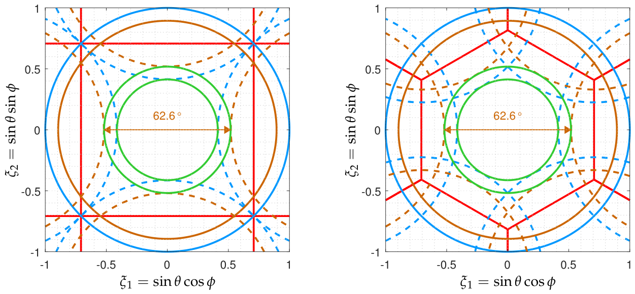
Referring back to Equation (1), in many synthesis imaging situations, the spatial frequencies ${\mathbf{u}}_{pq}\equiv {\mathbf{b}}_{pq}/\lambda$ match with the sampling nodes of a regular grid with a sampling step $d/\lambda$ in the Fourier domain, where d is the shortest distance between the elementary antennas of the array. This section aims at determining values of $d/\lambda$ compatible with a given field of view, regardless of the number of elementary antennas and their placement in the array (that will be addressed in Section 4), but provided that this arrangement results in a regular, Cartesian, or hexagonal sampling grid. According to the theory of discrete Fourier transform over periodic lattices [50] that was initiated in crystallography (chap. 2 in [51]), in such a case the shape (and the extent) of the field of view seen by the array of elementary antennas at instrument level, after synthesis imaging has been performed with the aid of a computer, is that of the elementary cell of the dual sampling grid in the direction cosines domain. When the Fourier sampling grid is Cartesian, the synthesized field of view at instrument level in the direction cosines domain is a square with side $\Delta \xi =\lambda /d$. Likewise, when this sampling grid is hexagonal, the synthesized field of view is a hexagon with a side-to-side extent $\Delta \xi =2\lambda /\sqrt{3}d$. As a consequence, owing to the factor $2/\sqrt{3}\simeq 1.15$, the same extent $\Delta \xi$ can be obtained with a square field-of-view or with a hexagonal one, but with a larger sampling step $d/\lambda$ in this latter case. Although this study aims at illustrating the impact of a $15\%$ increase of $d/\lambda$ on the preliminary design of synthetic aperture imaging radiometers like those onboard FRESCH and HAPS, this section concentrates on the revisit time and on the required imaging swath. The schematic geometry of SMOS observations shown in Figure 1 in [52] is a very nice illustration of the relationship between the elevation of a platform, the orientation of an antenna array with respect to the nadir direction, the range of local incidence angles, and the imaging swath.

3.1. FRESCH

For a satellite in orbit around the Earth at an elevation $h=750$ km, celestial mechanics [53] with the current reference ellipsoid of the World Geodetic System (WGS84) [54] tells us that the swath of the field-of-view should be as wide as 924 km to ensure a revisit time less than 3 days at the equator. This is precisely one of the imaging constraints imposed on the FRESCH project by scientists.

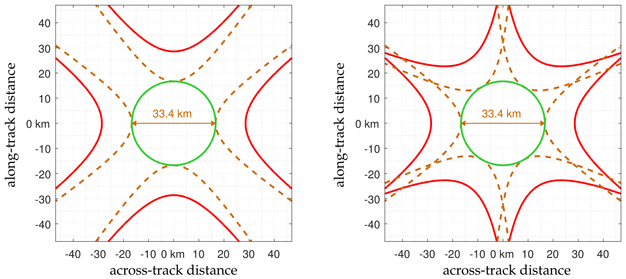
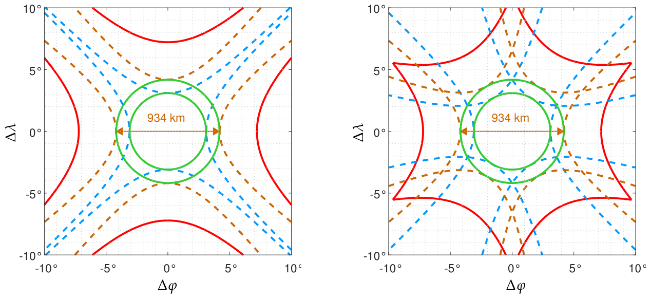
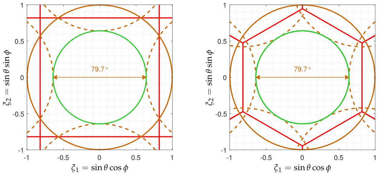
Shown in Figure 2 is the field of view seen at instrument level in the direction cosines domain by an array of elementary antennas from an elevation of 750 km above the Earth’s surface when the baseline vectors match with the sampling nodes of a Cartesian grid with a sampling step $d=0.707\lambda$, or with those of a hexagonal grid with a larger sampling step $d=0.816\lambda$. In both cases, the array points to the nadir direction, and the extent of the synthesized field of view $\Delta \xi$ is about $1.414$. Owing to the values of these sampling steps, which do not respect the Shannon sampling theorem [55,56], this imaged field of view is subject to field aliasing. Referring back to the expressions of $\Delta \xi$, very simple geometrical considerations for rejecting aliases outside the synthesized field-of-view show that $d/\lambda$ should be smaller than $1/2$ for a square field-of-view and smaller than $\sqrt{3}/3$ for a hexagonal one. In both cases, the extent of the region that is free from any Earth alias is about $1.039$. As illustrated in Figure 3, where the same field of view is shown at ground level, the Earth alias-free extent translates into a swath as wide as 934 km; that is to say, the required value of 924 km plus margins of 5 km on each side. Referring back to Figure 1, this value is not set in stone, as it may evolve to satisfy the final constraints imposed by scientists and to take into account appropriate margins.

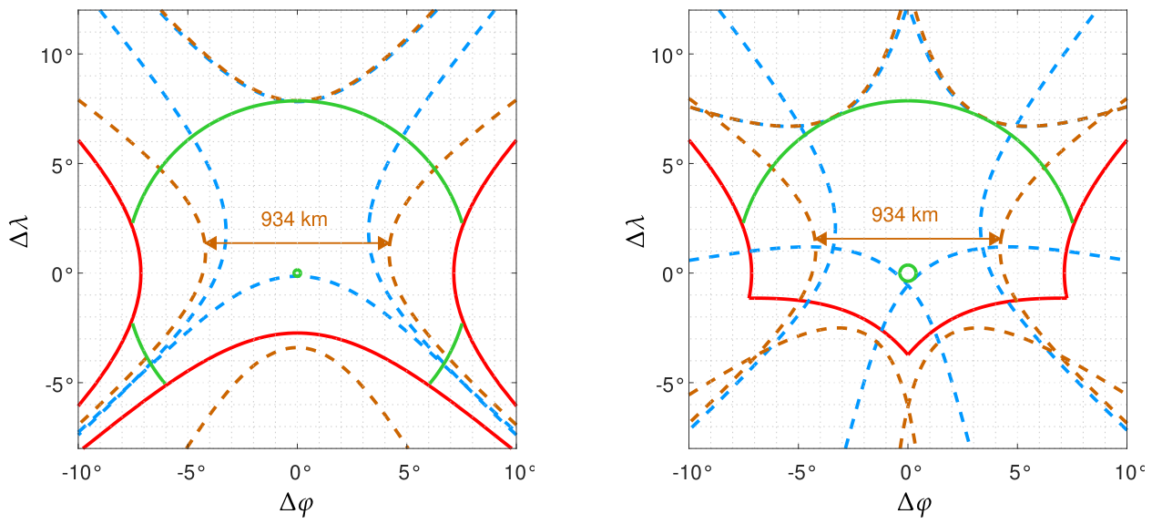
However, as a consequence of an array that is pointing to nadir, the range of incidence angles at ground level is limited to 35.5° in the Earth alias-free region of the synthesized field of view. To increase this value, the array must be tilted with respect to the nadir direction. This is what is shown in Figure 4 and Figure 5, where the range of available incidence angles at ground level is extended up to 55°, another constraint imposed on FRESCH by scientists. The consequence of this requirement is the inclination of the array relative to the nadir direction in the orbital plane with an angle $\alpha$ set to 22.9° for the Cartesian approach and to 25.9° for the hexagonal one, while refining the sampling step d to $0.71\lambda$ and to $0.82\lambda$ at the same time in order to maintain the ground swath to the previous value, including the margins. Moreover, there is a small margin for these settings, as the sub-satellite point is well inside the sky alias-free region, another constraint imposed by the lessons learned from the SMOS mission [57].

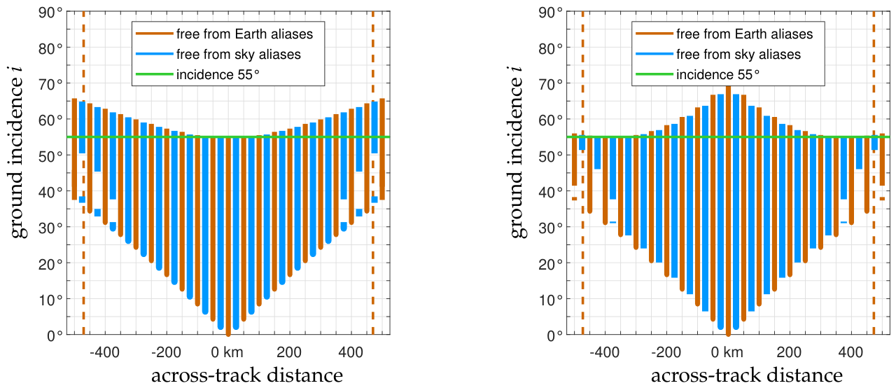
Finally, the distributions of the incidence angles i at ground level along dwell lines parallel to the satellite’s footprint as functions of the across-track distance are shown in Figure 6 for these two fields of view. The main difference between the two cases is for the ground incidence angles larger than 55°. On the one hand, when aliasing is governed by a Cartesian geometry, ground incidence angles along-track cannot exceed 55° in the Earth alias-free area, but at a distance from the satellite’s footprint, they can be as large as 65°. On the other hand, if aliasing is the result of a hexagonal geometry, ground incidence angles along the track can be as large as 70° in the Earth alias-free region, but at a distance from the satellite’s footprint, they cannot exceed 55°. Within the swath, the lowest ground incidence angle that is free from any Earth aliasing grows linearly with the across-track distance at the rate of about 7.5° every 100 km, whatever the geometry governing field aliasing. This is expected because when comparing the shape of the alias-free field of view at instrument level in Figure 4 or at ground level in Figure 5, the left and right aliases are almost the same. This is not the case for the top and bottom ones, in as much as when aliasing is governed by a hexagonal geometry, two aliases at the top and another two at the bottom are concerned, whereas in the Cartesian case there is only one alias at the top and another one at the bottom.

3.2. HAPS

For an aircraft, the situation slightly differs from that of a satellite in orbit. Indeed, in order to maintain a constant flight level, it must hold a null pitch angle; otherwise, the altitude will permanently change, and that will affect the synthesized field of view as well as the spatial resolution, both of which will vary from one snapshot to another. As a consequence, any array of elementary antennas installed onboard this aircraft will point to the nadir direction. The tilt angle $\alpha$ is therefore no longer a free parameter to consider for the design of an optimal configuration: its value is set and frozen to 0°. As illustrated by Figure 3 in [27], a typical HAPS operational altitude is around 20 km (i.e., 65,000 feet or flight level FL650), where a wind speed minimum is reached at this elevation.

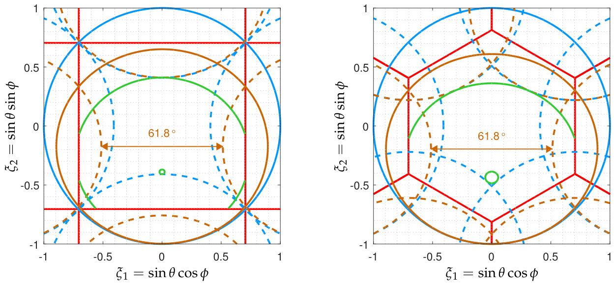
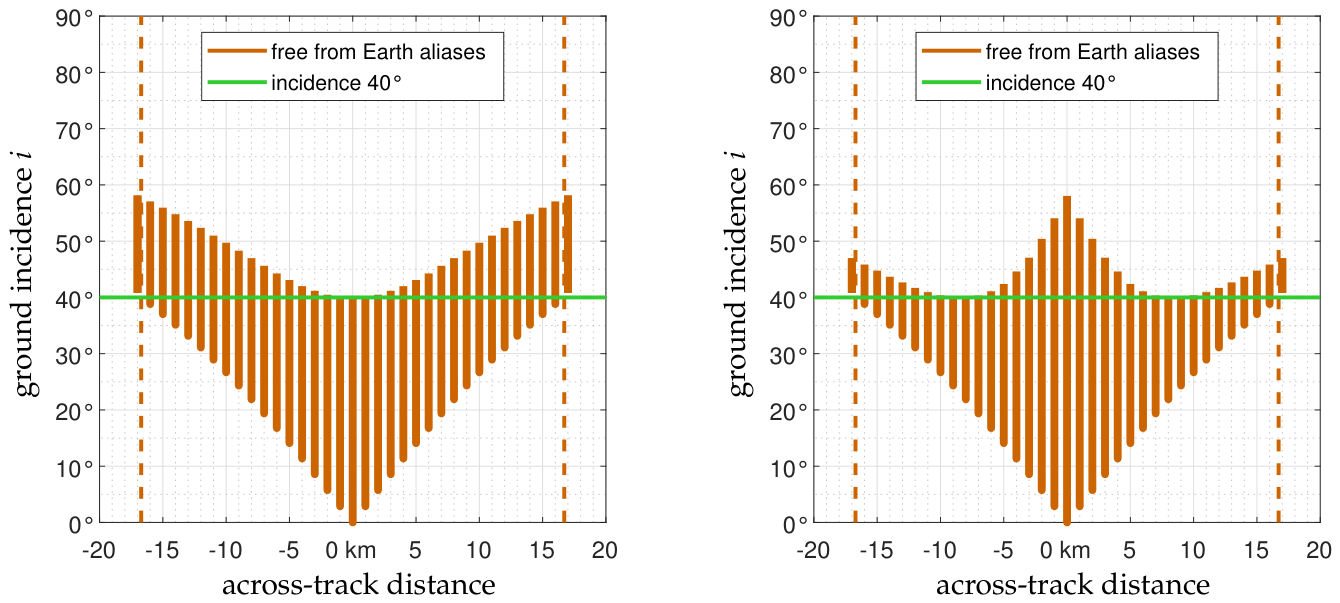
Shown in Figure 7 is the field-of-view seen at instrument level in the direction cosines domain by an array of elementary antennas from an elevation $h=20$ km above the Earth’s surface when the baseline vectors match with the sampling nodes of a Cartesian grid with a sampling step $d=0.611\lambda$ or with those of a hexagonal grid with a larger sampling step $d=0.705\lambda$. In both cases, the array points to the nadir direction, and the extent of the synthesized field of view $\Delta \xi$ is about 1.638. The extent of the region that is free from any Earth alias is only about 1.282. As illustrated on Figure 8, where the same field of view is shown now at ground level, this Earth alias-free extent translates into a swath as wide as 33.4 km. As a consequence of the orientation of the array that is pointing to the nadir direction, the range of incidence angles at ground level is limited to 40° in the Earth alias-free region of the synthesized field of view. This value is nevertheless in line with the constraints imposed by scientists.

Finally, the distributions of the incidence angles i at ground level along dwell lines parallel to the aircraft’s footprint as functions of the across-track distance are shown in Figure 9 for these two fields of view. The main difference between the two cases is for the ground incidence angles larger than 40°. On the one hand, when aliasing is governed by a Cartesian geometry, ground incidence angles along-track cannot exceed 40° in the Earth alias-free area. Conversely, if aliasing is the result of a hexagonal geometry, ground incidence angles along the track can be as large as 57° in the Earth alias-free region. Within the swath, the lowest ground incidence angle free from any Earth aliasing grows linearly with the across-track distance at the approximate rate of 2.5°/km, irrespective of the geometry governing field aliasing. Here, again, the reason has to be found in the locations of the aliases involved in the shape of the alias-free fields-of-view at instrument level in Figure 7 or at ground level in Figure 8.

4. Spatial Resolution

The resolution of a synthetic aperture imaging radiometer is driven by the length of the longest baselines of the antenna array. As soon as the geometry of the array and the spacing d between the antennas have been chosen to satisfy the ground swath constraint, this second step aims at setting the number $N_a$ of elementary antennas to meet the scientific requirements in terms of resolution. Before going into the details of this choice, a few clarifications should be given on the “resolution”. The angular resolution is an intrinsic and self-sufficient property of the array, as it does not vary in the synthesized field of view. On the contrary, the spatial resolution evaluated at ground level strongly depends on the local incidence angle. This is why the latter is often given in the nadir direction, where the ground incidence is reduced to zero.

4.1. FRESCH

When accounting for an expected ground resolution of ∼10 km without apodization, it turns out that the arms of any sparse antenna array should be as long as ∼9 m if the elevation is set to $h=750$ km. The lessons learned from SMOS with 3 arms leading to a star-shaped Fourier frequency coverage (i.e., a concave polygon) have motivated the choices to study solutions leading to convex frequency coverages. Although the hexagon is an attractive solution [58], the deployment of a hexagonal array in space is a complex and risky task, owing to the connection between both ends of the 6 arms. This is not the case of the $\times$-shaped and $+$-shaped arrays hereafter, which all lead to a square-shaped Fourier frequency coverage and whose deployment of the 4 arms (each one having a free end) does not raise any particular difficulty, given the experience acquired with the 3 arms of SMOS.

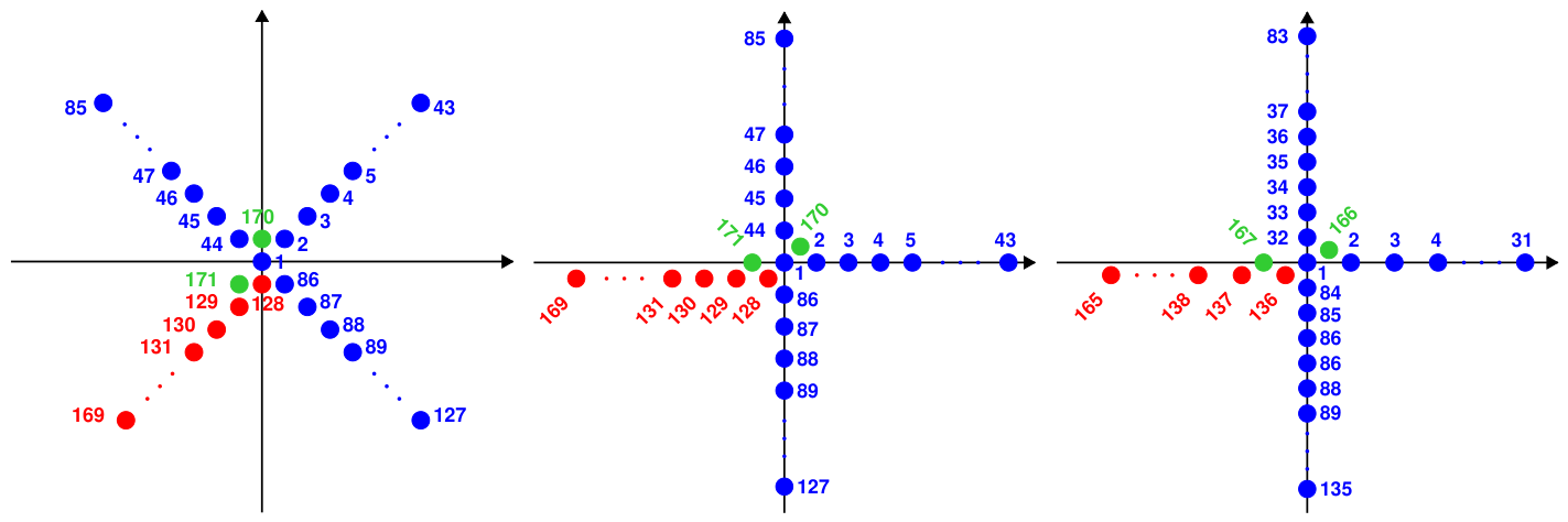
Shown in Figure 10 are three possible antenna arrays that have been taken into account in the preliminary studies of FRESCH. The initial one is a $\times$-shaped array populated with $N_a=171$ elementary antennas operating in the L-band at the central frequency $\nu =1413.5$ MHz ($\lambda \simeq 212$ mm). This number includes two additional antennas in order to meet the redundancy requirement for being calibrated with the aid of the Redundant Spacing Calibration (RSC) method [59]. The elementary antennas are regularly spaced every $\sqrt{2}d\simeq 213$ mm along the 4 arms of length $42\sqrt{2}d\simeq 8.94$ m, and one arm is judiciously shifted with respect to the others so that the shortest spacing between the closest antennas is reduced down to $d=0.71\lambda \simeq 151$ mm. This design that increases the extent of the field of view and therefore reduces the aliasing has been patented [60]. As shown in Figure 11, the Fourier frequency coverage of this array exhibits a square-shaped (with 4 extensions perpendicular to the sides) underlying a Cartesian sampling grid on which aperture synthesis operations have to be performed. The longest baseline between ${\mathcal{A}}_{85}$ and ${\mathcal{A}}_{127}$ is about $17.89$ m long. On the perpendicular arms, the longest baseline between ${\mathcal{A}}_{43}$ and ${\mathcal{A}}_{169}$ is slightly shorter with $17.78$ m. However, these baselines have almost no impact on the resolution, which is driven by the radius of the circle circumscribed to the square-shaped frequency coverage: the longest baseline contained in this circle is about $12.65$ m long (between ${\mathcal{A}}_{85}$ and ${\mathcal{A}}_{169}$). The second antenna array is nothing but the initial one after a 45° clockwise rotation, which is necessary for reducing the computational cost of digital beam forming [61], if this paradigm is selected for synthesis imaging [62]. Consequently, the underlying sampling grid of the Fourier frequency coverage is no longer a Cartesian one, but it is now a quincunx one, as illustrated in Figure 11. However, from the imaging properties point of view, these two configurations do not differ one from the other except by this 45° clockwise rotation, as detailed in [61]. This is the case, for example, for the field aliasing properties, which are those shown on the left side of Figure 4 and Figure 5. This is why only the initial one will be considered hereafter and compared to the alternative approach shown in Figure 10. This new configuration is inspired by the previous one, as it is again a $+$-shaped array populated with 167 elementary antennas. However, here the antennas are spaced every $d=0.82\lambda \simeq 174$ mm along two arms of length $52d\simeq 9.04$ m and every $\sqrt{3}d\simeq 301$ mm along two arms of length $30\sqrt{3}d\simeq 9.04$ m, with one of these two arms still being shifted with respect to the others. As shown in Figure 11, the Fourier frequency coverage of this array is very similar to the previous one, with again a square-shaped Fourier frequency coverage (with 4 extensions perpendicular to the sides), but it is now underlying a hexagonal sampling grid. Consequently, the field aliasing properties of this array are those shown on the right side of Figure 4 and Figure 5. The longest baseline between ${\mathcal{A}}_{83}$ and ${\mathcal{A}}_{135}$ is about $18.09$ m long. On the perpendicular arms, the longest baseline between ${\mathcal{A}}_{31}$ and ${\mathcal{A}}_{165}$ is again slightly shorter with $17.92$ m. However, these baselines have almost no impact on the resolution, which is driven by the radius of the circle circumscribed to the square-shaped frequency coverage: the longest baseline contained in this circle is about $12.74$ m long (between ${\mathcal{A}}_{83}$ and ${\mathcal{A}}_{165}$). Although the difference is small, it has to be noticed that this alternative approach exhibits a $0.7\%$ finer resolution compared to the initial one with $12.65$ m.

Referring back to Figure 11, the total number of points $N_f$ in the Fourier frequency coverage is equal to 14,535 for the two arrays populated with $N_a=171$ elementary antennas. This number slightly decreases down to 14,439 when keeping only those points in the circumscribed circle of radius $12.65$ m. In either case, this is much lower than the number of baselines $N_b$, which is equal to $N_a\times (N_a-1)$ = 29,070, as a consequence of redundant pairs of antennas. Likewise, the total number of points in the Fourier frequency coverage of the alternative array equipped with 167 elementary antennas is equal to 12,871. Here, again, this number slightly decreases down to 12,777 when keeping only those points in the circumscribed circle of radius $12.74$ m. Both have to be compared to the number of baselines, which is here equal to $167\times (167-1)$ = 27,722. Denoting by $\rho (u_f,v_f)$ the redundancy of each point $(u_f,v_f)$ in the Fourier frequency coverage, the values of $N_f$ have to be compared to those of $N_f^{\prime }$ defined by the discrete sum (2) in [58] such that:

$$N_f^{\prime }=\sum _{f=1}^{N_f}{\displaystyle \frac{1}{\rho (u_f,v_f)}}$$

(5)

which is the number of points in the Fourier frequency coverage when their redundancies $\rho (u_f,v_f)$ are taken into account, contrary to $N_f$, which does not take them into account. By definition, $\rho (u_f,v_f)\ge 1$. It is therefore obvious that $N_f^{\prime }\le N_f$ (equality is reached for fully non-redundant arrays [63] for which $\rho (u_f,v_f)=1$ for every point in the Fourier frequency coverage). It turns out that $N_f^{\prime }$ is here equal to 13,893 for the arrays populated with $N_a=171$ elementary antennas and to 12,244 for the array equipped with 167 antennas. These numbers slightly decrease down to 13,878, resp. 12,229, when keeping only those points in the circumscribed circles of radius $12.65$ m, resp. $12.74$ m.

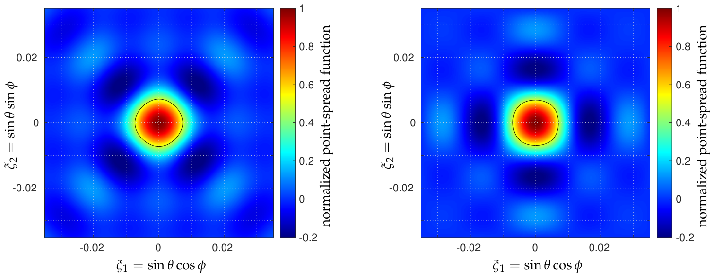
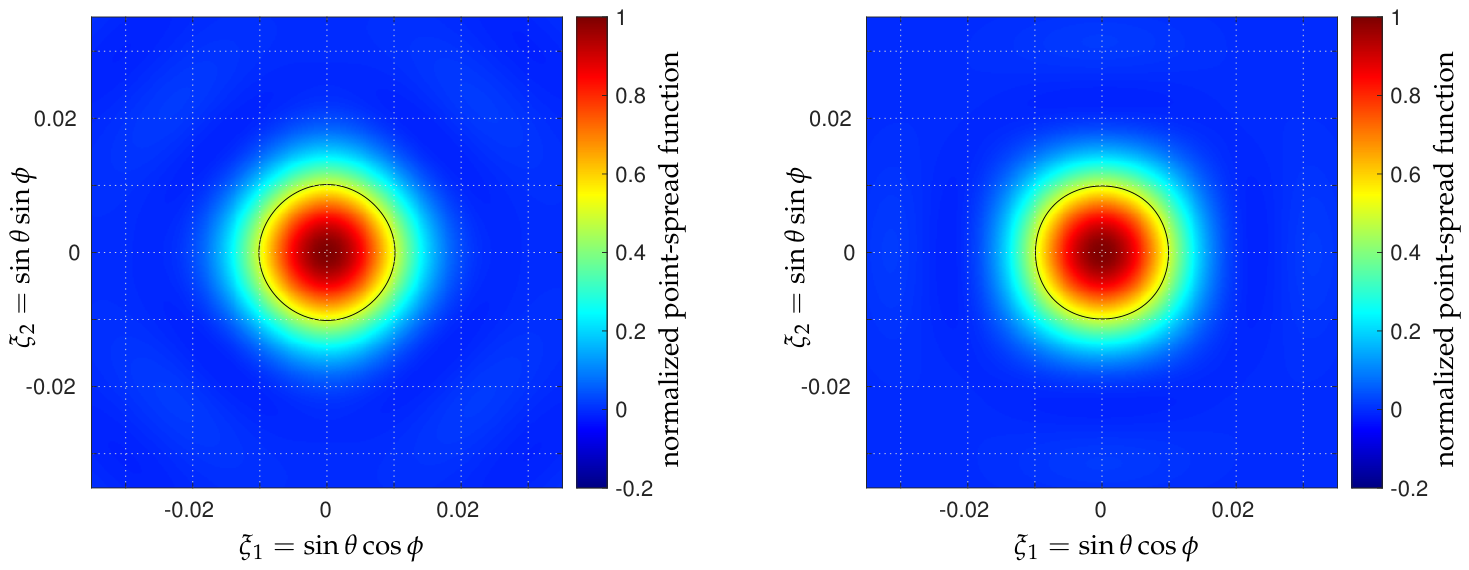
Finally, shown in Figure 12 are the point-spread functions at the instrument level in the direction cosines domain of the previous arrays. Owing to a similar shape of the Fourier frequency coverage and to very close dimensions of the arms, it is not surprising to obtain comparable angular resolutions: 0.824° for the initial array and 0.817° for the alternative one. When accounting for the elevation of the orbit, these numbers translate into $10.8$ km and $10.7$ km at ground level, respectively. As a consequence of the sharp frequency cut-off caused by the finite and limited extent of the frequency coverage in the Fourier domain, high-level side-lobes are clearly visible in the direction cosines domain. In order to reduce them, an apodization window might be necessary. Shown in Figure 13 are the corresponding responses when a Blackman window is used. The angular resolution at the instrument level is now about 1.153° for the initial array and about 1.144° for the alternative one. At ground level, these numbers translate into a resolution of $15.1$ km and $15.0$ km, respectively. All these figures of merit are summarized in

Table 1. Parameters and spatial resolution of FRESCH.

array	initial $\times$ or $+$		alternative $+$
h	750 km
$\alpha$	22.9°		25.9°
d	$0.71\lambda \simeq 151$ mm		$0.82\lambda \simeq 174$ mm
$N_a$	171		167
$N_b$	29,070		27,722
${\mathbf{b}}_{max}$	17.89 m	12.65 m	18.09 m	12.74 m
$N_f$	14,535	14,439	12,871	12,777
$N_f^{\prime }$	13,893	13,878	12,244	12,229
resolution (no window)	0.824°/10.8 km		0.817°/10.7 km
resolution (Blackman)	1.153°/15.1 km		1.144°/15.0 km

together with the relevant parameters introduced in this section.

As the satellite moves on its orbit, any given area in the synthesized field of view is observed in successive locations along so-called dwell lines parallel to the sub-satellite track. Although these areas are restricted to the Earth alias-free field of view, these dwell lines cross the contours of constant incidence angles i over a range of values that becomes larger as one comes nearer to the sub-satellite track, as illustrated by Figure 6. As a consequence, after synthesis imaging has been performed with the aid of a computer to inverse the complex visibilities, multi-angular profiles of brightness temperatures are available [64]. However, for obvious geometrical reasons, the ground resolution along these profiles is not constant because it varies with the incidence angle, contrary to the angular resolution, which remains constant in the field of view. It is therefore of great interest to have an idea of the disparity of the ground resolution along these dwell lines. Before going into the details of these variations, it is worth noting that the circular $-3$ dB contours of the point-spread functions, like those shown in Figure 12 and Figure 13, degenerate into ellipses as soon as they are projected on the Earth’s surface. A measure of how distinct an ellipse is from a circle is the aspect ratio, which is defined as the quotient $a/b$ between the longest and the shortest axis of the ellipse. Likewise, the equivalent disk diameter of an ellipse is defined as the geometric mean $\sqrt{ab}$.

Figure 12. Closed view of the normalized point-spread functions corresponding to the Fourier frequency coverages of Figure 11. The (solid black) contour at half-maximum value is a circle of diameter 0.824° for the initial array (left) and 0.817° for the alternative one (right). When accounting for the elevation of the satellite, $h=750$ km, these angular values translate into a ground resolution of 10.8 km and 10.7 km, respectively.

Figure 12. Closed view of the normalized point-spread functions corresponding to the Fourier frequency coverages of Figure 11. The (solid black) contour at half-maximum value is a circle of diameter 0.824° for the initial array (left) and 0.817° for the alternative one (right). When accounting for the elevation of the satellite, $h=750$ km, these angular values translate into a ground resolution of 10.8 km and 10.7 km, respectively.

Figure 13. Same as Figure 12 but with a Blackman apodization window. The (solid black) contour at half-maximum value is a circle of diameter 1.153° for the initial array (left) and 1.144° for the alternative one (right). When accounting for the elevation of the satellite, $h=750$ km, these angular values translate into a ground resolution of $15.1$ km and $15.0$ km, respectively.

Figure 13. Same as Figure 12 but with a Blackman apodization window. The (solid black) contour at half-maximum value is a circle of diameter 1.153° for the initial array (left) and 1.144° for the alternative one (right). When accounting for the elevation of the satellite, $h=750$ km, these angular values translate into a ground resolution of $15.1$ km and $15.0$ km, respectively.

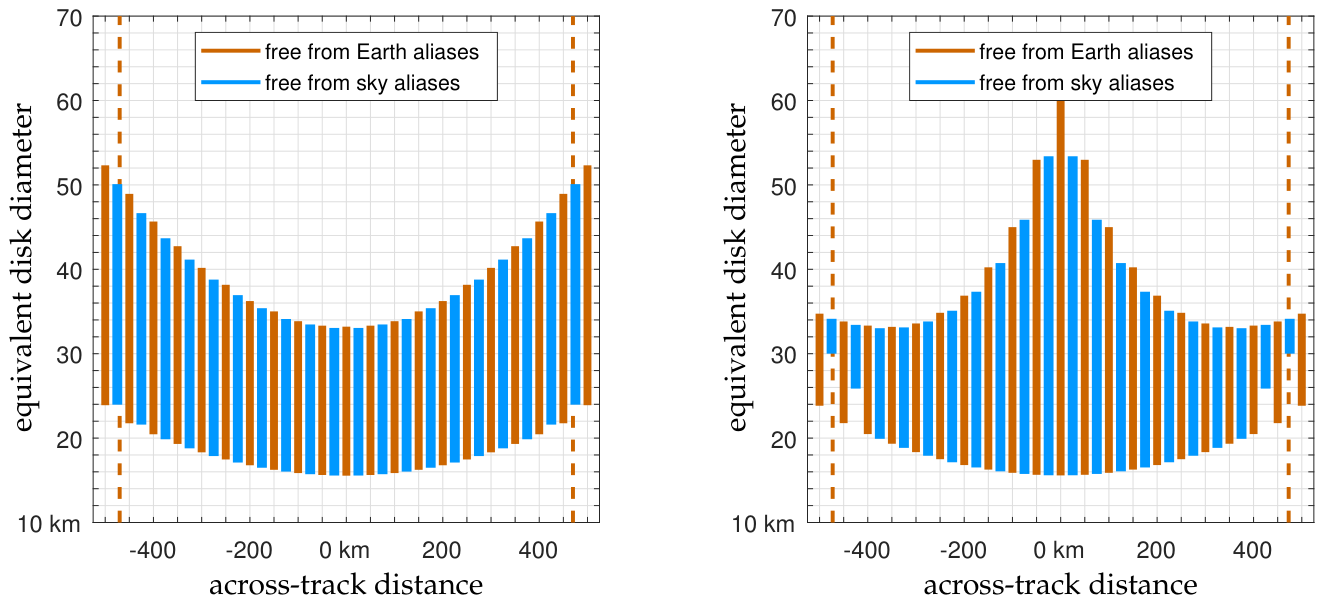
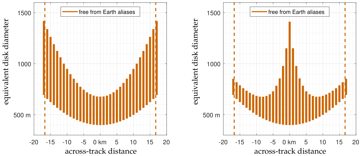
Shown in Figure 14 and Figure 15 are the range of values taken by the equivalent disk diameter and by the aspect ratio of the ground resolution along dwell lines parallel to the sub-satellite track. Referring back to Figure 6, the main difference between the two cases is for the ground incidence angles larger than 55°. On the one hand, when aliasing is governed by a Cartesian geometry, the range of the equivalent disk diameter varies from 15.1 km to 33.2 km along track and from 21.8 km to 48.9 km along a dwell line at 450 km from the sub-satellite track. At the same time, the ellipse aspect ratio varies from almost 1 to 1.9 along the track and from 1.3 and 2.7 along the same dwell line at 450 km from the sub-satellite track. On the other hand, if aliasing is the result of a hexagonal geometry, the range of the equivalent disk diameter varies from 15.0 km to 65.1 km along the track and from 21.8 km to 33.8 km along a dwell line at 450 km from the sub-satellite track. At the same time, the ellipse aspect ratio varies from almost 1 to 3.5 along the track and from 1.3 and 1.9 along the same dwell line at 450 km from the sub-satellite track.

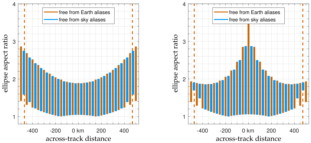
Finally, shown in Figure 16 and Figure 17 are the distributions of the equivalent disk diameter and of the ellipse aspect ratio in the fields-of-view shown in Figure 5. It is obvious that both are increasing functions of the ground incidence angle. As an example, the ground resolution is almost circular in the footprint direction of the satellite, with a diameter of about 15 km. Conversely, in the forward directions pointed by the arrays with an incidence angle of 55°, it is elliptical with an equivalent disk diameter of the order of 35 km and an aspect ratio of about 2, whatever the antenna array configuration. It should be noted that the alternative $+$-shaped array does not point to the backward direction with the same incidence angle of 55°, whereas the original $\times$-shaped array does. However, it is very likely that these directions will not be used, although they are free from Earth aliasing. Indeed, the equivalent disk diameter is larger than 45 km (i.e., 3 times the best resolution), and the aspect ratio is bigger than 3.5.

4.2. HAPS

With regard to HAPS, the situation is slightly different from that of FRESCH because the constraints for an air-borne instrument are not the same as those of a space-borne one. Owing to the environment, from the geometry point of view, only a ⊤-shaped array can be considered, the dimensions of the arms being constrained by the possibilities of accommodation in the wings (≲9.5 m) and along the body (≲8.5 m) of the HAPS.

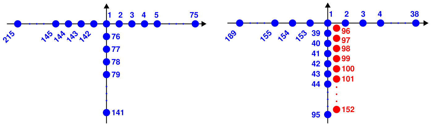
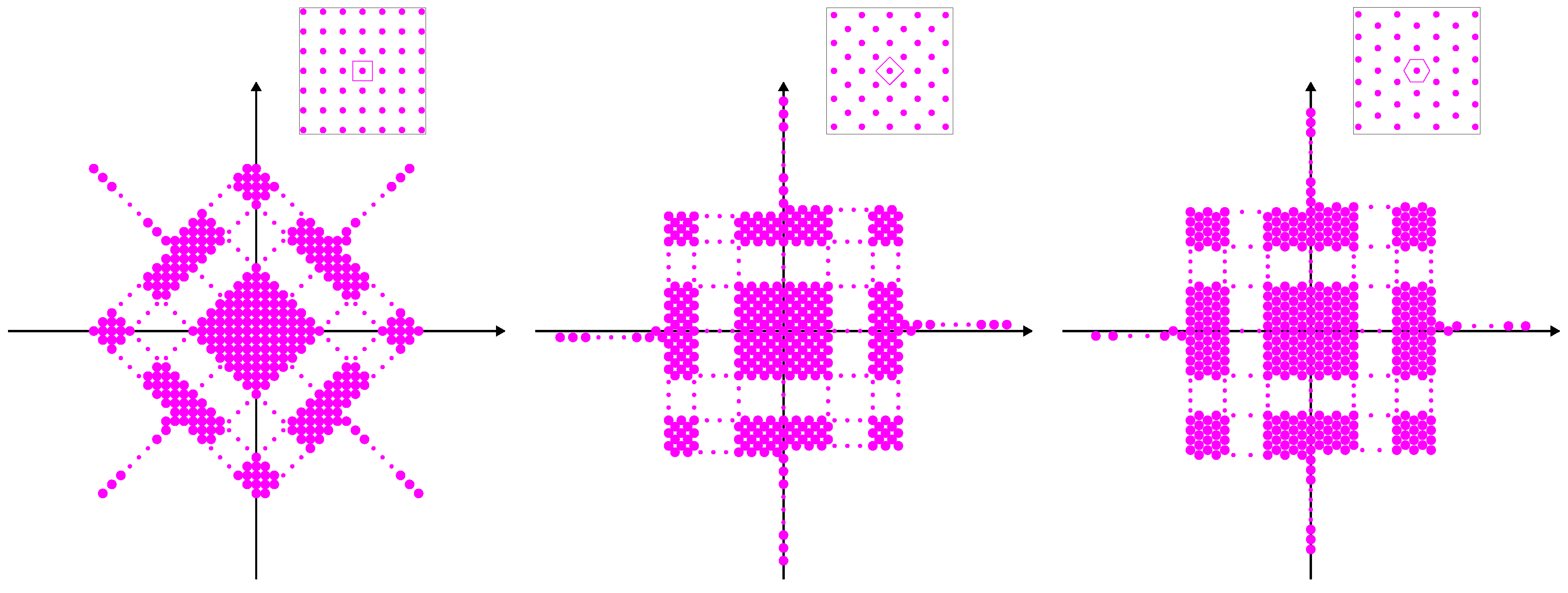
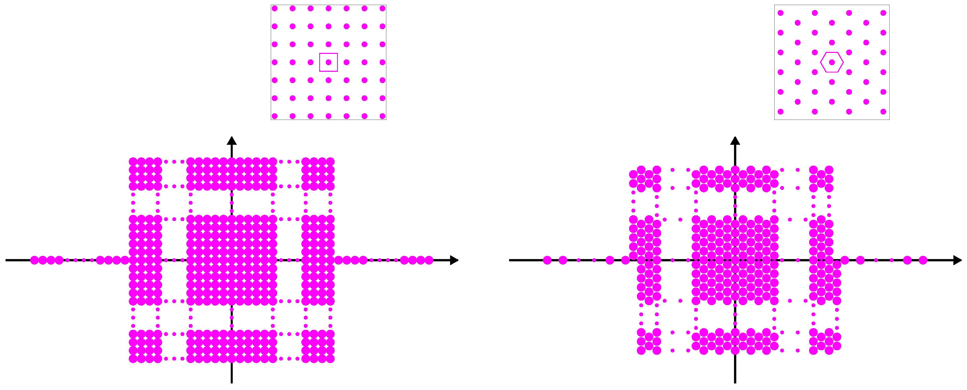
Shown on Figure 18 are two possible configurations that can be accommodated by the aircraft for operating at L-band the central frequency $\nu =1413.5$ MHz ($\lambda \simeq 212$ mm). With a total number of $N_a=215$ elementary antennas regularly spaced every $d=0.611\lambda \simeq 129.5$ mm along the 3 arms, the dimensions of the arms are $74d\simeq 9.58$ m across-track and $66d\simeq 8.55$ m along track for the disposition inducing Cartesian sampling grids. Likewise, with only $N_a=189$ elementary antennas and a short spacing of $d=0.705\lambda \simeq 149.5$ mm, they are equal to $37\sqrt{3}d\simeq 9.58$ m across-track and $57d\simeq 8.52$ m along-track for the configuration leading to hexagonal sampling. As shown in Figure 19, the Fourier frequency coverage of these two arrays exhibits a square-shaped (with 2 extensions across-track, i.e., along the wings of the aircraft). The first has an underlying Cartesian sampling grid on which aperture synthesis operations have to be performed. The longest baseline between ${\mathcal{A}}_{75}$ and ${\mathcal{A}}_{215}$ is about $19.17$ m. However, this baseline has almost no impact on the resolution, which is driven by the radius of the circle circumscribed to the square-shaped frequency coverage: the longest baseline contained in this circle is about $12.84$ m long (between ${\mathcal{A}}_{75}$ and ${\mathcal{A}}_{141}$ and also between ${\mathcal{A}}_{141}$ and ${\mathcal{A}}_{215}$). The second configuration is inspired by what has been found for FRESCH with the alternative $+$-shaped array while satisfying the accommodations onboard an aircraft that only allow 3 arms. However, 4 arms are necessary to obtain a Fourier frequency coverage underlying a hexagonal sampling grid. As a consequence, the fourth arm is here folded along the third one in the body of the aircraft. The antennas are spaced every $d=0.705\lambda \simeq 149.5$ mm along the body of the aircraft and every $\sqrt{3}d\simeq 259$ mm along the two wings. The longest baseline between ${\mathcal{A}}_{38}$ and ${\mathcal{A}}_{189}$ is about 19.17 m. However, here again this baseline has almost no impact on the resolution, which is driven by the radius of the circle circumscribed to the square-shaped frequency coverage: the longest baseline contained in this circle is about 12.87 m long (between ${\mathcal{A}}_{152}$ and ${\mathcal{A}}_{189}$).

Referring back to Figure 19, the total number of points $N_f$ in the Fourier frequency coverage is equal to 19,965 for the array populated with $N_a=215$ elementary antennas. This number slightly decreases down to 19,869 when keeping only those points in the circumscribed circle of radius $12.84$ m. This is much lower than the number of baselines $N_b$, which is equal to $N_a\times (N_a-1)$ = 46,010, as a consequence of redundant pairs of antennas. Likewise, the total number of points in the Fourier frequency coverage of the alternative array equipped with 189 elementary antennas is equal to 17,249. Here, again, this number slightly decreases down to 17,201 when keeping only those points in the circumscribed circle of radius $12.87$ m. Both have to be compared to the number of baselines, which is here equal to $189\times (189-1)$ = 35,532. Referring back to (5), it turns out that $N_f^{\prime }$ is here equal to 19,558 for the array populated with $N_a=215$ elementary antennas and to 16,791 for the array equipped with 189 antennas. These numbers slightly decrease down to 19,549, resp. 16,784, when keeping only those points in the circumscribed circles of radius $12.84$ m, resp. $12.87$ m.

Figure 18. Two ⊤-shaped arrays for HAPS: (left) $N_a=215$ elementary antennas regularly spaced every $d=0.611\lambda \simeq 129.5$ mm along the 3 arms and leading to Cartesian sampling grids, (right) $N_a=189$ elementary antennas with a short spacing $d=0.705\lambda \simeq 149.5$ mm and inducing hexagonal sampling grids.

Figure 18. Two ⊤-shaped arrays for HAPS: (left) $N_a=215$ elementary antennas regularly spaced every $d=0.611\lambda \simeq 129.5$ mm along the 3 arms and leading to Cartesian sampling grids, (right) $N_a=189$ elementary antennas with a short spacing $d=0.705\lambda \simeq 149.5$ mm and inducing hexagonal sampling grids.

Figure 19. Fourier frequency coverage of the two ⊤-shaped arrays of Figure 18 with an underlying sampling grid (left) or with a hexagonal one (right). In both case, the closed view highlights the shape of the elementary cell of the sampling grid: square (left) and hexagon (right).

Figure 19. Fourier frequency coverage of the two ⊤-shaped arrays of Figure 18 with an underlying sampling grid (left) or with a hexagonal one (right). In both case, the closed view highlights the shape of the elementary cell of the sampling grid: square (left) and hexagon (right).

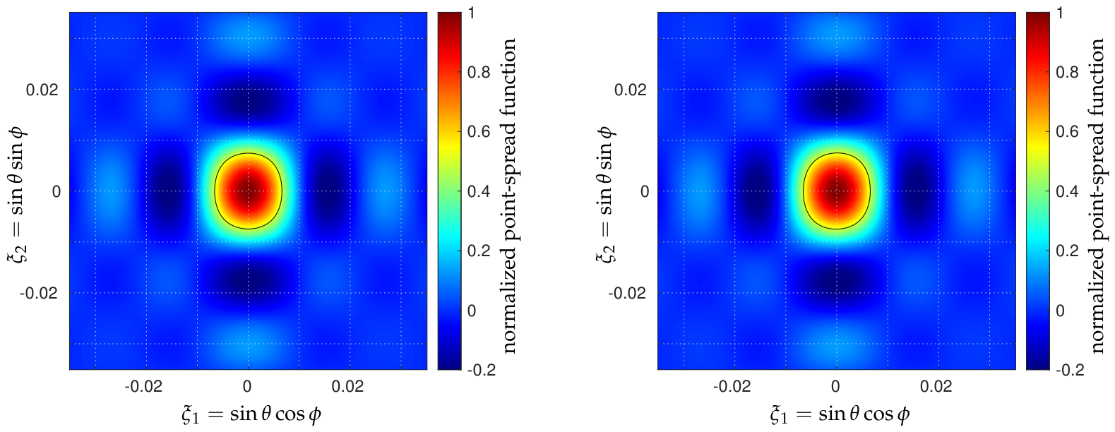
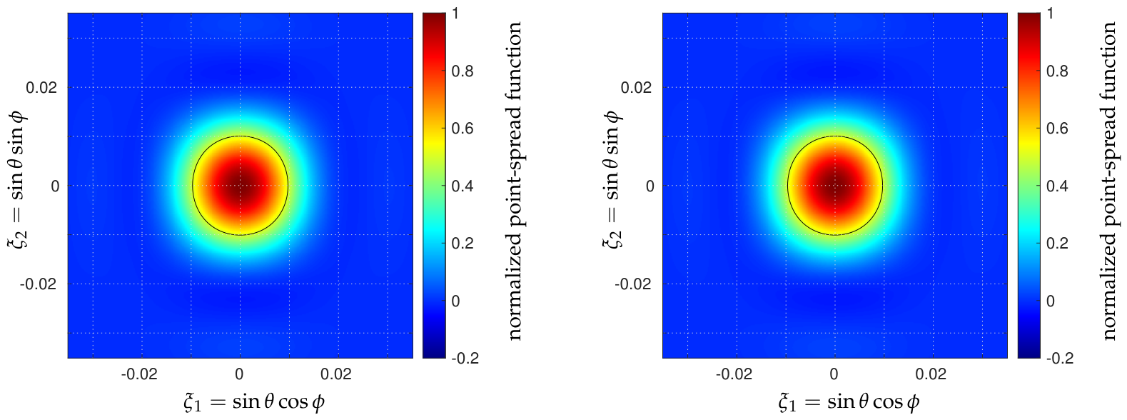
Finally, shown in Figure 20 are the point-spread functions at instrument level in the direction cosines domain of the previous arrays. Owing to the very similar shape and extent of the Fourier frequency coverage, it is not surprising to obtain comparable angular resolutions. However, owing to arms of different lengths, it is not centrosymmetric: it is about 0.772° across-track with two arms about $9.5$ m long each and about 0.875° along-track with an arm about $8.5$ m long. When accounting for the flying elevation of the aircraft, $h=20$ km, the ground resolution in the Nadir direction is about 269 m across-track and slightly less than 305 m along-track (the diameter of the equivalent disk is about 286 m). Here, again, high-level side-lobes are clearly visible in the direction cosines domain. In order to reduce them, an apodization window might be necessary. Shown in Figure 21 are the corresponding responses when a Blackman window is used. The angular resolution at instrument level is now about 1.122° across-track and 1.166° along-track. At ground level, these numbers translate into 392 m across-track and 407 m along-track (the diameter of the equivalent disk is about 399 m). All these figures of merit are summarized in Table 2 together with the relevant parameters introduced in this section.

Although the aircraft flies at an altitude well lower than that of a satellite in orbit, with therefore a closer horizon, there is still great interest in having an idea of how the ground resolution varies along dwell lines. Shown in Figure 22 and Figure 23 are the range of values taken by the equivalent disk diameter and by the aspect ratio of the elliptical ground resolution along dwell lines parallel to the ground track of the aircraft. Referring back to Figure 9, the main difference between the two arrays is for the ground incidence larger than 40°. On the one hand, when aliasing is governed by a Cartesian geometry, the range of the equivalent disk diameter varies from 399 m to 677 m along track and from 624 m to 1265 m along a dwell line at 15 km from the ground track of the aircraft. At the same time, the ellipse aspect ratio varies between almost 1 and slightly less than $1.8$ along the track and from $1.5$ to $3.3$ along the same dwell line at 15 km from the footprint of the aircraft. On the other hand, if aliasing is the result of a hexagonal geometry, the range of the equivalent disk diameter varies from 399 m to 1415 m along the track and from 624 km to 788 m along a dwell line at 15 km from the ground track of the aircraft. At the same time, the ellipse aspect ratio varies between almost 1 and $3.7$ along the track and from $1.7$ to $2.0$ along the same dwell line at 15 km from the footprint of the aircraft.

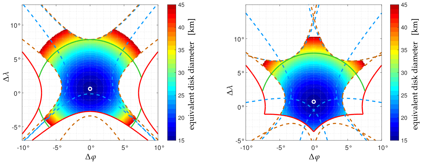
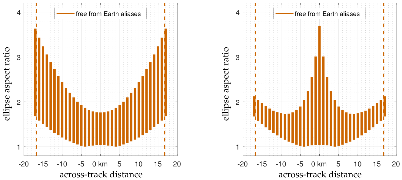
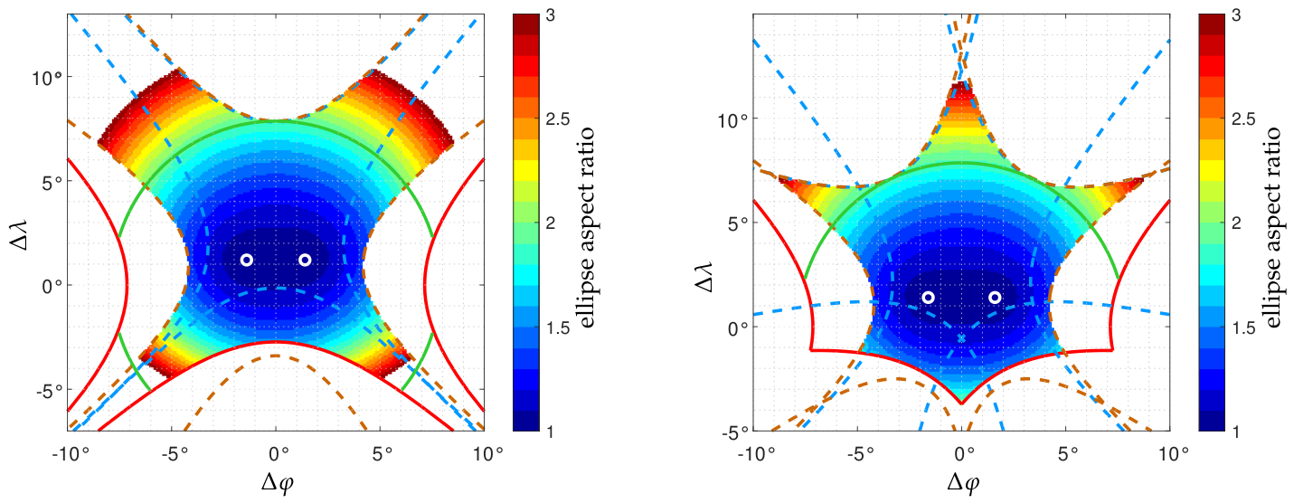
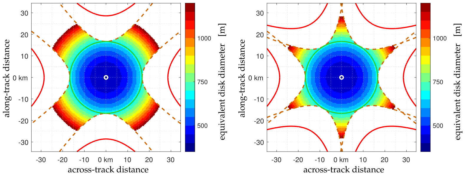
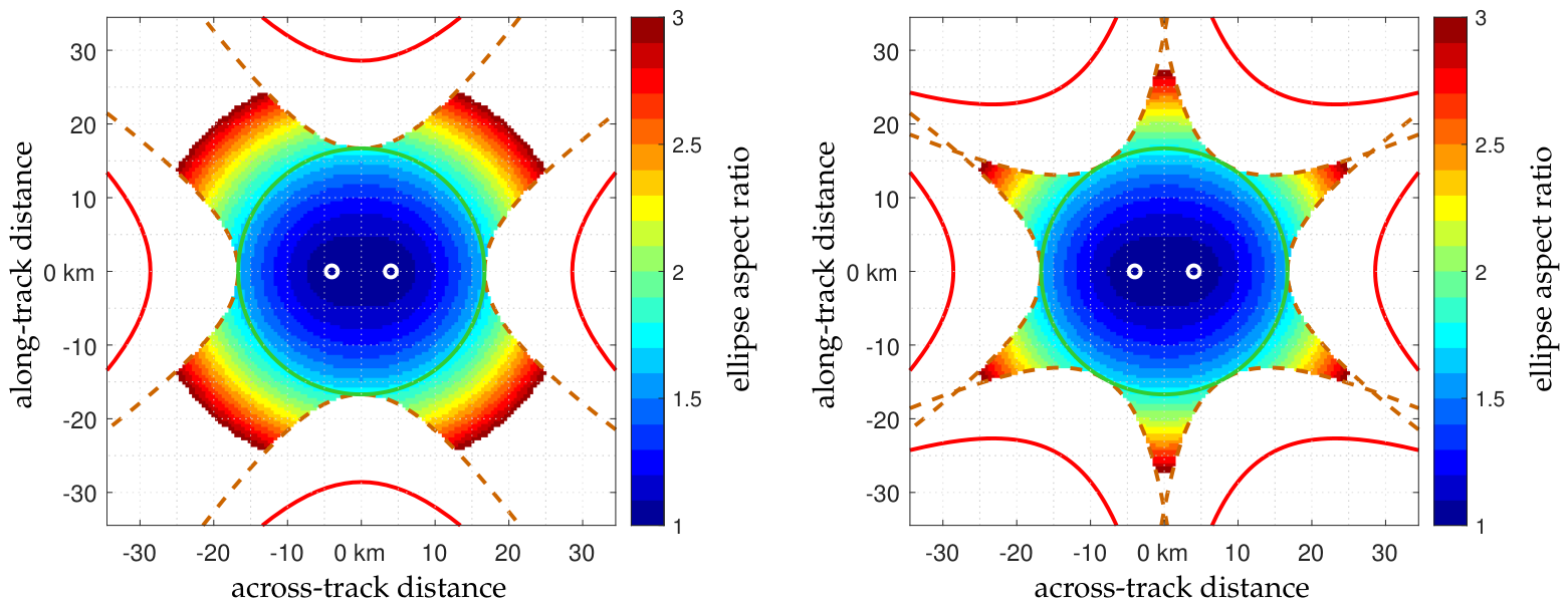
Finally, shown in Figure 24 and Figure 25 are the distributions of the equivalent disk diameter and of the ellipse aspect ratio in the fields-of-view shown in Figure 8. Here, again, despite a lower elevation compared to that of FRESCH, both are increasing functions of the ground incidence angle. However, owing to the absence of a tilt of the arrays ($\alpha =0^{°}$), here the variations are centrosymmetric with respect to the nadir direction, where the ground resolution is almost circular. On the contrary, for a ground incidence angle i = 40°, the equivalent disk diameter of the elliptical ground resolution is about 620 m with an aspect ratio slightly less than 1.8.

Figure 24. Distribution of the equivalent disk diameter of the $-3$ dB contour of the point-spread functions of Figure 21 after being projected at ground level, here only in the Earth alias-free field-of-view of Figure 8 synthesized by the arrays of Figure 18: initial ⊤-shaped array (left) with Cartesian sampling and alternative array (right) with hexagonal sampling. The white circle is the location where this diameter is the smallest one: about 365 m in both cases. It is an increasing function of the incidence angle i: about 620 m for i = 40° (green contour).

Figure 24. Distribution of the equivalent disk diameter of the $-3$ dB contour of the point-spread functions of Figure 21 after being projected at ground level, here only in the Earth alias-free field-of-view of Figure 8 synthesized by the arrays of Figure 18: initial ⊤-shaped array (left) with Cartesian sampling and alternative array (right) with hexagonal sampling. The white circle is the location where this diameter is the smallest one: about 365 m in both cases. It is an increasing function of the incidence angle i: about 620 m for i = 40° (green contour).

Figure 25. Distribution of the ellipse aspect ratio of the $-3$ dB contour of the point-spread functions of Figure 21 after being projected at ground level, here only in the Earth alias-free field-of-view of Figure 8 synthesized by the arrays of Figure 18: initial ⊤-shaped array (left) with Cartesian sampling and alternative array (right) with hexagonal sampling. The white circles are the locations where this ratio is equal to 1 (i.e., the ellipse is a circle). It is an increasing function of the incidence angle i: the longest axis of the ellipse is about 1.8 times longer than the shortest one for i = 40° (green contour).

Figure 25. Distribution of the ellipse aspect ratio of the $-3$ dB contour of the point-spread functions of Figure 21 after being projected at ground level, here only in the Earth alias-free field-of-view of Figure 8 synthesized by the arrays of Figure 18: initial ⊤-shaped array (left) with Cartesian sampling and alternative array (right) with hexagonal sampling. The white circles are the locations where this ratio is equal to 1 (i.e., the ellipse is a circle). It is an increasing function of the incidence angle i: the longest axis of the ellipse is about 1.8 times longer than the shortest one for i = 40° (green contour).

Table 2. Parameters and spatial resolution of HAPS.

array	initial ⊤		alternative ⊤
h	65,000 feet/20 km
$\alpha$	0°
d	$0.611\lambda \simeq 129.5$ mm		$0.705\lambda \simeq 149.5$ mm
$N_a$	215		189
$N_b$	46,010		35,532
${\mathbf{b}}_{max}$	19.17 m	12.84 m	19.17 m	12.87 m
$N_f$	19,965	19,869	17,249	17,201
$N_f^{\prime }$	19,558	19,549	16,791	16,784
resolution (no window)	0.772° × 0.875°/269 m × 305 m
resolution (Blackman)	1.122° × 1.166°/392 m × 407 m

Table 2. Parameters and spatial resolution of HAPS.

array	initial ⊤		alternative ⊤
h	65,000 feet/20 km
$\alpha$	0°
d	$0.611\lambda \simeq 129.5$ mm		$0.705\lambda \simeq 149.5$ mm
$N_a$	215		189
$N_b$	46,010		35,532
${\mathbf{b}}_{max}$	19.17 m	12.84 m	19.17 m	12.87 m
$N_f$	19,965	19,869	17,249	17,201
$N_f^{\prime }$	19,558	19,549	16,791	16,784
resolution (no window)	0.772° × 0.875°/269 m × 305 m
resolution (Blackman)	1.122° × 1.166°/392 m × 407 m

5. Radiometric Sensitivity

In microwave imaging by aperture synthesis, the radiometric sensitivity is frequently a critical issue, especially when the motion of the platform limits the integration time available for synthesizing an image from interferometric measurements. When inverting complex visibilities V in the presence of radiometric noise, at the end of the synthesis imaging process, the radiometric sensitivity $\Delta T$ in the boresight direction $\mathsf{\xi }=0$ is given by Equation (1) in [58] as:

$$\Delta T\left(0\right)=S_{uv}{\displaystyle \frac{T_A+T_R}{\sqrt{B{\tau }_{eff}}}}{\displaystyle \frac{4\pi }{D}}{\alpha }_w^{\phantom{2}}\sqrt{N_f^{\prime }}.$$

(6)

In the others directions, as explained in [65], $\Delta T$ varies according to the relation:

$$\Delta T\left(\mathsf{\xi }\right)=\Delta T\left(0\right){\displaystyle \frac{\sqrt{1-{\mathsf{\xi }}^2}}{\langle {\mathcal{F}}_n^2\left(\mathsf{\xi }\right)\rangle }},$$

(7)

where $\langle {\mathcal{F}}_n^2\left(\mathsf{\xi }\right)\rangle$ is the average normalized power pattern of the elementary antennas. In these expressions, $S_{uv}$ is the area of the elementary cell of the sampling grid in the Fourier domain (${(d/\lambda )}^2$ for a Cartesian sampling, $\raisebox{1ex}{$\sqrt{3}$}\!\left/ \!\raisebox{-1ex}{$2$}\right.{(d/\lambda )}^2$ for a hexagonal sampling), ${\tau }_{eff}$ is the effective time of integration, B is the noise bandwidth, and D is the directivity of the elementary antennas (so that according to Equation (2-144) in [66], $4\pi /D$ is nothing but the corresponding beam solid angle $\mathrm{\Omega }$) and $N_f^{\prime }$ is the number of points in the Fourier frequency coverage as defined by (5).

As detailed in [66], for a fixed wavelength $\lambda$, the larger an antenna, the higher is its directivity. As a consequence, owing to a longer spacing between the elementary antennas allowing a wider collecting area, the antennas of the alternative arrays inducing hexagonal sampling grids will have a higher directivity, and therefore a smaller solid angle, than those of the original arrays leading to Cartesian sampling grids. Moreover, part of this additional space between the elementary antennas can be used to reduce antenna coupling. In every case, numerical simulations have been conducted with CST Studio [67]. Four dual-polarized 3D-printed antenna elements were designed for operation in the protected L-band with a resonant frequency set to $1413.5$ MHz. The use of additive manufacturing enables lightweight structures and precise fabrication while maintaining good electromagnetic performance. The antennas were developed with different aperture sizes to investigate their suitability for integration within the interferometric array. Referring back to Table 1 and Table 2, the physical dimensions of the antennas are $174\times 174\times 5.6$ mm³ and $151\times 151\times 5.6$ mm³ for the FRESCH case, and $149.5\times 149.5\times 5.1$ mm³ and $129.5\times 129.5\times 5.1$ mm³ for the HAPS one. No particular optimization has been performed with regard to the geometry as well as with the choice of the materials because it is not the purpose of this study. As a consequence, the values of D used in this comparison can certainly be improved, and the solid angles $\mathrm{\Omega }$ reduced accordingly for the benefit of the radiometric sensitivity.

The effect of the apodization window W is taken into account with the term ${\alpha }_w^{\phantom{2}}$, which is defined by relation (16) in [68]:

$${\alpha }_w^2={\displaystyle \frac{1}{N_f}}\sum _{f=1}^{N_f}{W}^2(u_f,v_f).$$

(8)

By definition, $W(u_f,v_f)\le 1$ so that ${\alpha }_w^{\phantom{2}}\le 1$ (equality is reached for the rectangular window only for which $W(u_f,v_f)=1$ for every point $(u_f,v_f)$ in the Fourier frequency coverage).

Finally, according to Equation (12.19) in [69], the noise temperature of the elementary antennas $T_A$ is the weighted average of the equivalent brightness temperature of the observed scene $T_{scene}$ and the physical (or ambient) temperature $T_{phys}$ of the antennas:

$$T_A=\eta T_{scene}+(1-\eta )T_{phys},$$

(9)

where the radiation efficiency $0<\eta <1$ is a measure of how much power is lost in the antennas, as defined by Equation (12.9) in [69]. Likewise, according to Equation (10.12) in [69], the receiver’s noise temperature $T_R$ is related to the physical (or ambient) temperature $T_{phys}$:

$$T_R=T_{phys}({10}^{NF/10}-1),$$

(10)

where $NF>0$ dB is the noise figure of the receivers, as defined by Equation (10.10) in [69].

Among the many parameters contributing to the estimation of the radiometric sensitivity, the effective integration time ${\tau }_{eff}$ is a dimensioning one, and it deserves special attention. In the words of Le Vine in [70], “sensitivity is an especially critical issue for measurements from low Earth orbit because the motion of the platform limits the integration time available for forming an image.” Referring back to (6), the integration time has to be as long as possible. However, in order to reduce the smearing effects [71] in the retrieved brightness temperature maps caused by the motion of the antenna array with respect to the observed scene [72], it has to be short enough. Unlike in [70], where “the integration time is chosen to be the time available per resolution cell,” the largest integration time at instrument level ${\tau }_{inst}$ is here defined as the time required for the point on the Earth’s surface in the Nadir direction to move along-track a ground distance equal to one quarter of the resolution. Furthermore, this instrumental integration time is to be distinguished from the physical integration time ${\tau }_{phys}$, which is defined by the time during which the incidence angle i of a target in the same Nadir direction does not vary by more than a few degrees (1° or 2°, depending on the physical domain concerned by multi-angular brightness temperatures).

Finally, ${\tau }_{inst}$ and ${\tau }_{phys}$ also have to be distinguished from the effective integration time ${\tau }_{eff}$. If correlations were estimated in an analog way, ${\tau }_{eff}$ would be equal to ${\tau }_{inst}$ or ${\tau }_{phys}$. However, correlations are estimated numerically [73]. As a consequence, the quantization levels of the radio signals have to be taken into account. A detailed study was conducted a few years ago [74]. As intuitively expected, the degradation of the radiometric sensitivity with a digital correlator compared to what it is with an analog one decreases with the number of quantization levels. For example, in the worst case, the level of noise in a $2\times 2$ level digital correlator is $1.57$ times higher than in an analog correlator, which is a well-known theoretical result, i.e., $\pi /2$, that follows from a study by Van Vleck and Middleton [75]. This factor is about $1.23$ with a $3\times 3$ level digital correlator and less than $1.13$ with a $4\times 4$ level one. As a consequence, referring back to (6), with a 1 bit digital correlator, ${\tau }_{eff}$ is $1.{57}^2\simeq 2.46$ times shorter than ${\tau }_{inst}$ or ${\tau }_{phys}$. This is also what is reported in [68] for SMOS, which is equipped with a $2\times 2$ level digital correlator where only the sign of the radio signals being correlated matters. This reduction would be about $1.{23}^2\simeq 1.51$ with a $3\times 3$ level digital correlator and less than $1.{13}^2\simeq 1.28$ with a $4\times 4$ level digital correlator. The choice of the number of quantization levels in a digital correlator is therefore of great importance. To be complete on this subject, the comprehensive study recently conducted by radio astronomers from the National Radio Astronomy Observatory (NRAO) cannot be ignored [76]. The values of the quantization efficiency ${\eta }_Q^{\phantom{2}}$ found in Table 1 of this exhaustive study are reported hereafter in

Table 3. Degradation of integration time with the number of quantization levels.

number of levels of quantization	2	3	4	8	16	32	64	128	256
degradation of integration time	2.467	1.525	1.288	1.079	1.023	1.007	1.002	1.001	≃1

but under the expression $1/{\eta }_Q^2$ because it is nothing but the factor by which the integration time is degraded, more exactly shortened.

5.1. FRESCH

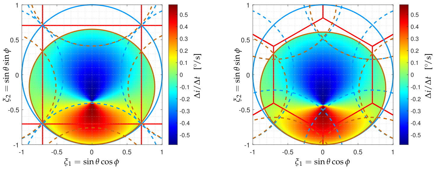
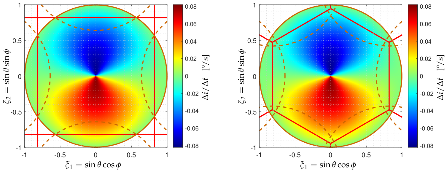
For a satellite in orbit around the Earth at an elevation $h=750$ km, the orbital speed $v_h$ is about $7.5$ km/s [53]. As a consequence, in the circular orbit approximation, the ground speed of the sub-satellite point $v_o=v_h\times R_{\oplus }/(R_{\oplus }+h)$ is close to $6.7$ km/s. Referring back to the previous section, the ground resolution has been estimated as 10 km without any apodization window. As a consequence, ${\tau }_{inst}$ is about $\raisebox{1ex}{$1$}\!\left/ \!\raisebox{-1ex}{$4$}\right.10/v_o\simeq 0.37$ s. However, if synthesis imaging had to be performed always at the resolution of a Blackman window with a ground resolution of 15 km, this time would be augmented up to $0.56$ s. Shown in Figure 26 is the rate of variation of the incidence angle in the fields of view shown in Figure 4. In every case, this rate is larger in the boresight direction $\mathsf{\xi }=0$ where $\Delta i/\Delta t\simeq 0.{57}^{°}$/s. As a consequence, depending on the accepted range of variation of the incidence angle i during integration, ${\tau }_{phys}$ may vary between $1/0.57\simeq 1.75$ s (with a 1° variation of i) and $2/0.57\simeq 3.50$ s (with a 2° variation).

Without entering into the details of the inversion of multi-angular profiles of brightness temperatures, the flight duration over the dwell lines shown in Figure 27 together with the range of ground incidence angles in Figure 6 is very helpful for understanding the underlying aspects of the integration time. For example, let us consider the footprint of the initial $\times$-shaped array with an overflight duration of about 175 s. If integration is performed at the instrument level, the number of brightness temperatures acquired over a given pixel of the footprint is $175/{\tau }_{inst}\simeq 310$, and they cover a range of incidence angles from 0° to 55°. Depending on the application, these incidence angles can be binned every 1° or every 2°. This is very similar to increasing the integration time up to ${\tau }_{phys}$ so that the number of brightness temperature samples reduces to $175/1.75\simeq 100$ or to $175/3.5\simeq 50$ over the same range of ground incidence angles. The question that arises then is whether it is better to invert a brightness temperature profile with many rather noisy data or if it is preferable to invert one with less data but less noise. The answer is clearly out of the scope of this study.

Complementarily, the fraction $(T_A+T_R)/\sqrt{B{\tau }_{eff}}$ in (6) is nothing but the standard deviation of the radiometric noise $\Delta V$ affecting the complex visibilities V. It does not depend on the shape of the antenna array, nor on the spacing between the elementary antennas, nor on their number or characteristics. On the contrary, the remaining terms $S_{uv}\mathrm{\Omega }{\alpha }_w\sqrt{N_f^{\prime }}$, whose product is nothing but the amplification factor $\mathrm{\Gamma }$ of the noise $\Delta V$ through the inversion process of V, strongly depend on this geometry as well as on the elementary antennas themselves. As shown in Figure 28, the directivity D obtained from simulations conducted with small antennas of physical dimensions $151\times 151\times 5.6$ mm³ for the initial $\times$-shaped array and with larger ones of physical dimensions $174\times 174\times 5.6$ mm³ for the alternative $+$-shaped array are, respectively, about $9.20$ dB and $9.56$ dB so that the corresponding solid angles $\mathrm{\Omega }=4\pi /D$ are about 1.51 sr and 1.39 sr. If $S_{uv}$ is larger for the alternative $+$-shaped array with 167 antennas than it is for the initial $\times$-shaped array of FRESCH with 171, it turns out that $\mathrm{\Omega }$, ${\alpha }_w$, and $N_f^{\prime }$ are smaller so that the amplification factor is almost the same: $\mathrm{\Gamma }\simeq 38.76$ for the initial $\times$-shaped array and $\mathrm{\Gamma }\simeq 38.51$ for the alternative $+$-shaped one. As a consequence, all other things being equal, both arrays will have the same behavior regarding the propagation of radiometric noise through the imaging process and will achieve very similar performances in terms of radiometric sensitivity with expected differences less than 1% on $\Delta T\left(0\right)$, to the benefit of the alternative array.

Finally, estimations of the radiometric sensitivity in the boresight direction with $\eta =0.93$, $NF=1.5$ dB, $B=24$ MHz, and $T_{phys}=293$ K (or 20 °C) for $T_{scene}=90$ K (a typical value over the ocean) and 250 K (over land) are given in

Table 4. Parameters and radiometric sensitivity of FRESCH.

array	initial $\times$ or $+$		alternative $+$
$d/\lambda$	0.710		0.820
$S_{uv}$	0.504		0.582
$N_f^{\prime }$	13,878		12,229
${\alpha }_w$	0.432		0.430
D	9.20 dB		9.56 dB
$\mathrm{\Omega }$	1.51 sr		1.39 sr
$T_{scene}$	90 K	250 K	90 K	250 K
${\tau }_{inst}$	$0.56$ s
	$2.38$ K	$3.96$ K	$2.36$ K	$3.93$ K	analog
$\Delta T\left(0\right)$	$3.74$ K	$6.21$ K	$3.71$ K	$6.17$ K	1 bit
	$2.70$ K	$4.49$ K	$2.68$ K	$4.46$ K	2 bits
${\tau }_{phys}$	$1.75$ s
	$1.35$ K	$2.24$ K	$1.34$ K	$2.22$ K	analog
$\Delta T\left(0\right)$	$2.12$ K	$3.51$ K	$2.10$ K	$3.49$ K	1 bit
	$1.53$ K	$2.54$ K	$1.52$ K	$2.52$ K	2 bits
${\tau }_{phys}$	$3.50$ s
	$0.95$ K	$1.58$ K	$0.94$ K	$1.57$ K	analog
$\Delta T\left(0\right)$	$1.50$ K	$2.49$ K	$1.48$ K	$2.47$ K	1 bit
	$1.08$ K	$1.80$ K	$1.07$ K	$1.78$ K	2 bits

for the integration times discussed here for FRESCH. It is not surprising that a radiometric sensitivity over the ocean close to $1.5$ K cannot be achieved at the snapshot level because ${\tau }_{inst}$ is too short. However, this value can be almost reached when compiling few snapshots with the same ground resolution over a longer integration time ${\tau }_{phys}$ during which the variations $\Delta i$ of the incidence angle i do not exceed 1° if a 2 bits/4 levels correlator is used, or with $\Delta i=2^{°}$ if only 1 bit/2 levels correlations are available. Keeping in mind that for many reasons correlations are nowadays estimated numerically [73], values with an analog correlator are just given for comparison as well as for understanding why correlators with more than 2 bits are not considered owing to the low benefit in regard to their cost.

5.2. HAPS

Regarding HAPS, the situation is here again slightly different from that of FRESCH because the flight dynamics of a satellite are not those of an aircraft evolving in the stratosphere at a flying altitude $h=20$ km. As detailed in Tables 1 and 2 in [77], a typical ground speed $v_o$ from such an elevation is about 31 m/s. Referring back to the previous section, the smallest ground resolution, the across-track one, has been estimated to be 246 m without any apodization window. As a consequence, ${\tau }_{inst}$ is here about $\raisebox{1ex}{$1$}\!\left/ \!\raisebox{-1ex}{$4$}\right.246/v_o\simeq 1.98$ s. However, if synthesis imaging had to be performed always at the resolution of a Blackman window with a ground resolution of 358 m, this time could be as long as 2.89 s. This is much longer ($5\times$) than for FRESCH as a consequence of evolving at a higher elevation with a faster ground speed, although the angular resolutions of FRESCH and HAPS reported in Table 1 and Table 2 are comparable. Shown in Figure 29 is the rate of variation of the incidence angle in the fields-of-view shown in Figure 7. In every case, this rate is larger in the boresight direction $\mathsf{\xi }=0$ where $\Delta i/\Delta t\simeq 0.08°$/s. This is much slower than for FRESCH ($7\times$), here again owing to a higher elevation and a faster ground speed. As a consequence, if the accepted range of variation of the incidence angle i is set to 1°, the physical integration time ${\tau }_{phys}$ can be as long as $1/0.08\simeq 12.5$ s, which improves the radiometric sensitivity by almost 2 compared to ${\tau }_{inst}$.

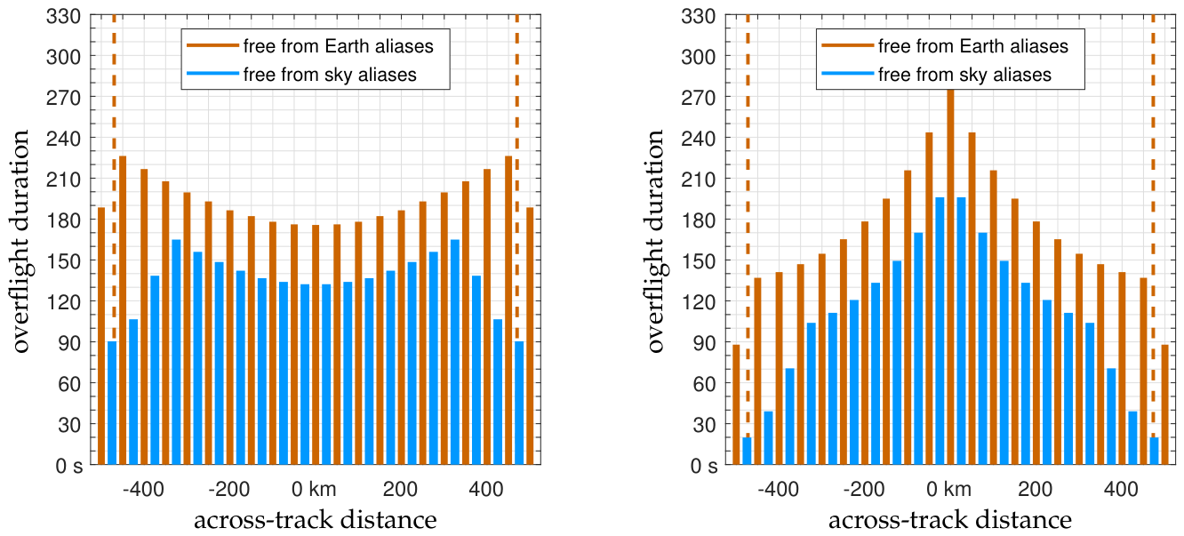
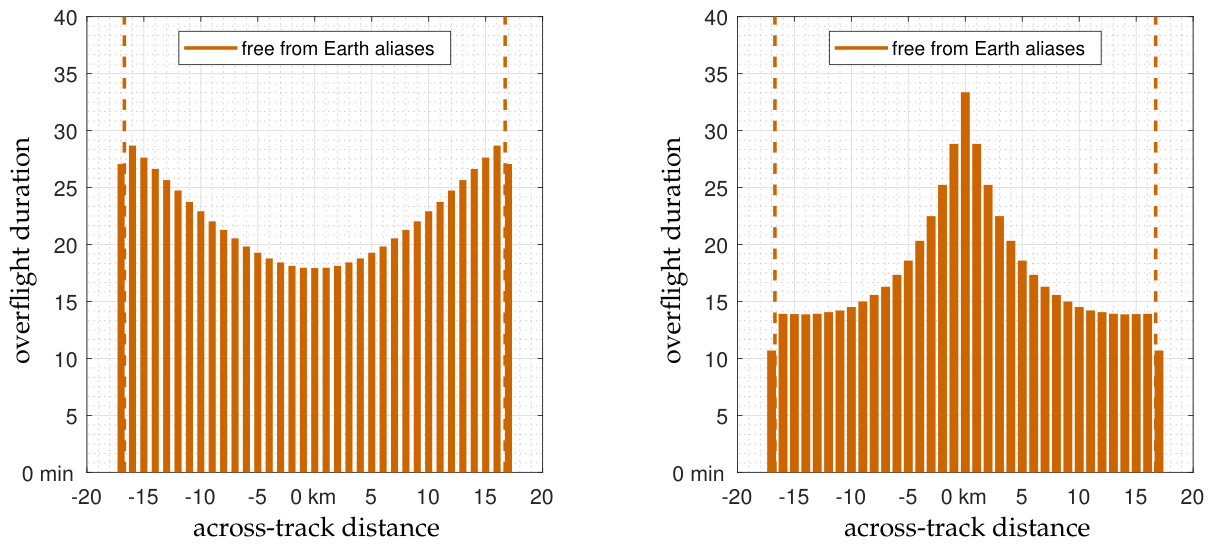
Here, also the flight duration over the dwell lines shown in Figure 30, together with the range of ground incidence angles in Figure 9, is very helpful for understanding the inversion of multi-angular profiles of brightness temperatures. For example, let us consider the footprint of the initial ⊤-shaped array with an overflight duration of about 18 min (the time for the aircraft to fly $33.4$ km at a ground speed $v_o=31$ m/s). If integration is performed at the instrument level, the number of brightness temperatures acquired over a given pixel of the footprint is $1080/{\tau }_{inst}\simeq 370$, and they cover a range of incidence angles from 0° to 40°.

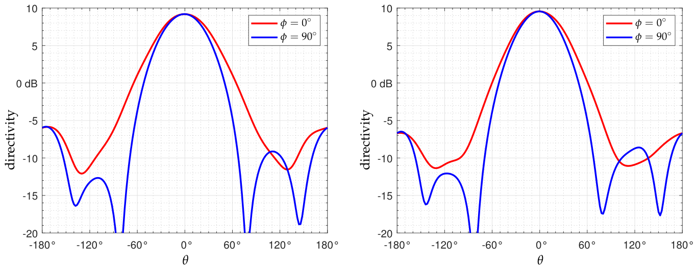
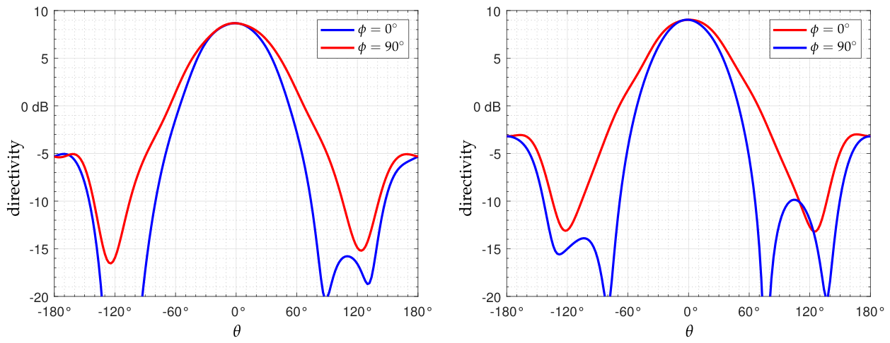
Finally, as shown in Figure 31, the directivity D obtained from simulations conducted with small antennas of physical dimensions $129.5\times 129.5\times 5.1$ mm³ for the initial ⊤-shaped array and with larger ones of physical dimensions $149.5\times 149.5\times 5.1$ mm³ for the alternative array are, respectively, about $8.67$ dB and $9.04$ dB so that the corresponding solid angles $\mathrm{\Omega }=4\pi /D$ are about $1.71$ sr and $1.57$ sr. Estimations of the radiometric sensitivity in the boresight direction with $\eta =0.93$, $NF=1.5$ dB, $B=24$ MHz, and $T_{phys}=293$ K (or 20 °C) for $T_{scene}=90$ K (a typical value over the ocean) and 250 K (over land) are given in

Table 5. Parameters and radiometric sensitivity of HAPS.

array	initial ⊤		alternative ⊤
$d/\lambda$	$0.611$		$0.705$
$S_{uv}$	$0.373$		$0.430$
$N_f^{\prime }$	$19,549$		$16,784$
${\alpha }_w$	$0.433$		$0.433$
D	$8.67$ dB		$9.04$ dB
$\mathrm{\Omega }$	$1.71$ sr		$1.57$ sr
$T_{scene}$	90 K	250 K	90 K	250 K
${\tau }_{inst}$	$2.89$ s
	$1.04$ K	$1.73$ K	$1.02$ K	$1.70$ K	analog
$\Delta T\left(0\right)$	$1.64$ K	$2.72$ K	$1.61$ K	$2.67$ K	1 bit
	$1.18$ K	$1.96$ K	$1.16$ K	$1.93$ K	2 bits

for the physical integration time discussed here for HAPS. Referring back to the estimation of the radiometric sensitivity of FRESCH, here again the area $S_{uv}$ is larger for the alternative ⊤-shaped array with 189 elementary antennas than it is for the initial one with 215. However, the remaining terms $\mathrm{\Omega }$, ${\alpha }_w$, and $N_f^{\prime }$ are smaller so that the amplification factor $\mathrm{\Gamma }$ is almost the same: ≃38.6 for the initial ⊤-shaped array and ≃37.9 for the alternative one. As a consequence, all other things being equal, both arrays will have the same behavior regarding the propagation of radiometric noise through the imaging process and will achieve very similar performances in terms of radiometric sensitivity with expected differences of about $2\%$ on $\Delta T\left(0\right)$, to the benefit of the alternative array.

6. Discussions

Regarding the shape and the extent of the synthesized field-of-view, the reader has probably noticed a difference between the two fields-of-view shown in Figure 7. On the one hand, when aliasing is governed by a Cartesian geometry, the synthesized field of view is a square. On the other hand, if aliasing is the result of a hexagonal geometry, it is a hexagon. In both cases, the side-to-side extent of the synthesized field of view is the same, $1.638$, as the result of an appropriate choice for the sampling step d. The radius of the circle circumscribed to these two synthesized fields-of-view is therefore equal to $1.638/\sqrt{2}\simeq 1.158$ for the square field-of-view and to $1.638/\sqrt{3}\simeq 0.946$ for the hexagonal one. As a consequence, it is evidence that some viewing directions in the four corners of the square-shaped field of view are pointing outside the unit circle with radius corresponding to $sin\theta =1$. As explained in [78], “the corresponding directions ξ have neither a physical meaning nor a mathematical one, as they correspond to situations where $sin\theta$ would be larger than 1. As a consequence, they cannot be taken into account in the inversion process.” One might think that it would be enough to simply set to zero the corresponding components of the retrieved brightness temperature maps $\tilde{T}$. However, it is well known that a function and its Fourier transform cannot both have a finite support unless this function is identically zero, as stated with different words by Bracewell (chap. 8 in [79]). As a consequence, $\tilde{T}$ cannot have its Fourier spectrum limited to the experimental frequency coverage and simultaneously be itself limited to a region of the synthesized field of view, here the intersection of the latter with the unit circle. The problem is deeper and the inversion of the complex visibilities V itself raises a difficulty, especially in presence of noise $\Delta V$, as detailed in [78]. Although the artifacts introduced by this unstable inversion can be filtered out, it is at the cost of additional time consuming linear algebra operations and only to some extent. Referring back to the ⊤-shaped arrays of Figure 18 and given that the hexagonal synthesized field-of-view in Figure 7 does not suffer from the same problem, the array with 189 elementary antennas spaced every $d=0.705\lambda \simeq 149.5$ mm on one arm and every $\sqrt{3}d\simeq 259$ mm along the two other arms is a valuable alternative to the original array with 215 antennas spaced every $d=0.611\lambda \simeq 129.5$ mm on each arm, especially since the number of elementary antennas is significantly reduced while the performances in terms of spatial resolution and radiometric sensitivity are maintained almost at the same level, if not better.

Referring back to the estimation of the radiometric sensitivity, in both illustrating cases only 24 MHz of the 1400–1427 MHz protected band [80] have been taken into account with 1.5 MHz margins on both sides. However, in order to reduce the decorrelation due to fringe-washing [40], as well as the degradation of the data caused by RFI contaminations [81], it might be necessary to decompose this bandwidth of interest into a few sub-bands [82] and to filter the signals kept by each elementary antenna with the aid of an appropriate polyphase filter bank [83]. Referring back to the time delay $t_{pq}$ defined just after Equation (1), such a decomposition is all the more true when the narrow-band condition $t_{pq}\ll 1/B$ is no longer satisfied [84]. This is precisely the case of FRESCH because for the original $\times$-shaped array as well as for the alternative $+$-shaped one, $t_{pq}$ can be as large as 60 ns, whereas the characteristic time $1/B$ is of the order of 42 ns. Decomposing the 24 MHz bandwidth of interest into 8 sub-bands of 3 MHz will augment this characteristic time up to 333 ns, which is more than 5 times larger than the maximum value taken by the time delay $t_{pq}$ for any baseline ${\mathbf{b}}_{pq}$ in any pointing direction $\mathsf{\xi }$. If sub-banding is the solution to decorrelation, it is not without consequence on synthesis imaging. Indeed, since the central wavelength of observation $\lambda$ will change from one sub-band to another, whereas the spacing d between the elementary antennas will not, the Fourier sampling step $d/\lambda$ will therefore vary from one sub-band to another. Coming back to this example where the 24 MHz bandwidth of interest is decomposed into 8 sub-bands of 3 MHz, the Fourier sampling step of the initial $\times$-shaped array of Figure 10 varies from 0.705 in the lowest sub-band centered on 1403 MHz up to 0.715 in the highest sub-band centered on 1424 MHz. As a consequence, in the lowest sub-band, the side-to-side extent of the synthesized field of view is as large as $1/0.705\simeq 1.418$ so that the radius of the circle circumscribed to this square is equal to $1.418/\sqrt{2}$, which is larger than 1, meaning that few viewing directions are pointing outside the unit circle. This is not the case of the alternative $+$-shaped array of Figure 10, for which the Fourier sampling step in the lowest sub-band is about 0.814 and the side-to-side extent of the synthesized field-of-view is also equal to 1.418, but thanks to a different geometry governing aliasing, the radius of the circle circumscribed to this hexagon is here equal to $1.418/\sqrt{3}\simeq 0.819$, which is well below 1. As a consequence, here also the alternative $+$-shaped array leads to hexagonal aliasing conditions and to hexagonal sampling grids is a valuable candidate for the antennas array of FRESCH.

Finally, to be complete with the estimation of the radiometric sensitivity, it should be noticed that the definition of the integration time ${\tau }_{inst}$ at snapshot level with the factor $\raisebox{1ex}{$1$}\!\left/ \!\raisebox{-1ex}{$4$}\right.$ is perhaps very conservative. Although enlarging it up to $\raisebox{1ex}{$1$}\!\left/ \!\raisebox{-1ex}{$2$}\right.$ is not conceivable, this fraction can be taken equal to $\raisebox{1ex}{$1$}\!\left/ \!\raisebox{-1ex}{$3$}\right.$ without significantly degrading the data by smearing effects. This would extend ${\tau }_{inst}$ by 33% and would result in a significant gain of 15% on the radiometric sensitivity, which could benefit the FRESCH and HAPS projects regardless of the antenna array selected for each one.

With regard to the numerical modeling of the instrument with Equation (1), beam forming is also a candidate for the observing paradigm of FRESCH [62], together with interferometry considered in this study. It is well-known that digital beam forming requires a larger amount of calculations onboard compared to interferometry, especially when the number of elementary antennas is large and the pointing direction are numerous. With regard to the initial $\times$-shaped array, a solution has been found for reducing this amount of calculations. As detailed in [61], the number of elementary operations [85] is reduced from 638 TMAC/s down to 16.5 TMAC/s thanks to a simple 45° clockwise rotation. The question therefore arises whether the alternative $+$-shaped array could benefit from this reduction or not. The answer is clearly yes, as the geometry of the two arrays is identical, with almost the same number of elementary antennas on the same arms. Making the same enumeration as the one made in [61], it turns out that the number of elementary operations is around 16.3 TMAC/s, as a result of a slightly lower number of antennas. The alternative $+$-shaped array is therefore fully compatible with the two aperture synthesis paradigms: interferometry and beam forming.

7. Conclusions

Nowadays, time-consuming end-to-end simulations are performed within the new paradigm of “co-design” [86] in which engineers, scientists, and end-users are actively involved. They play an ongoing role in assessing the sensitivity and the robustness of mission performances to driving parameters, to instrument errors, noises, and failures, as well as to onboard and ground data processing. As a consequence, they are at the heart of the decisions for making the necessary trade-offs between scientific requirements and technical/financial feasibility of a mission. Microwave imaging radiometers by aperture synthesis are no exception to this rule. This study was devoted to their key performances, foremost among which are the spatial resolution and the radiometric sensitivity, as well as the extent of the synthesized field of view that is free from any aliasing artifact. Emphasis was put on key parameters of the antenna array, such as its geometrical shape, the number of elementary antennas, and their spacing. They have to be chosen in a precise order, with the aim to meet the scientific specifications and at the same time to satisfy the engineering constraints. They can be adjusted iteratively but always in the same order: firstly the instrumental parameters that define the shape and the extent of the alias-free field of view, then those driving the spatial resolution, and finally those governing the radiometric sensitivity.

This optimization process has been illustrated with two specific examples chosen for serving as a common thread in this study: the $+$-shaped array selected for the Fine Resolution Explorer for Salinity, Carbon, and Hydrology (FRESCH) and a ⊤-shaped array onboard a High-Altitude Pseudo-Satellite (HAPS), two projects of high-resolution microwave imaging radiometers by aperture synthesis. In both cases this article has reported only one iteration of the optimization process, so the values of the instrumental parameters obtained at the end of this study, as well as the expected performances, are likely to evolve as soon as the collaborative approach produces results and converges to the final configuration. Indeed, the goal was not so much to give a final value for each parameter as to explain the approach and to show the path to be taken to achieve it. Another objective of this work was to evidence how it is possible to perform aperture synthesis on hexagonal sampling grids but with antenna arrays whose geometry naturally leads to Cartesian sampling grids, as is the case with elementary antennas regularly spaced along the perpendicular arms of ⊤, $+$, or $\times$-shaped arrays. The impact of the form factor $2/\sqrt{3}$ onto the synthesized field of view has been illustrated, and the absence of effect onto the spatial resolution as well as onto the radiometric sensitivity has been quantified. In any case, as soon as a hexagonal sampling concept is selected, the same instrumental performances can be achieved, but with fewer elementary antennas (and more spaced from each other) than necessary with a Cartesian approach. This reduction is not without interest in terms of the mass, power, and data rate budgets.

References

1. Pastorino, M. Microwave Imaging, 1st ed.; John Wiley & Sons: Hoboken, NJ, USA, 2010. [Google Scholar]
2. Ruf, C.S.; Swift, C.T.; Tanner, A.B.; Le Vine, D.M. Synthetic Aperture Microwave Radiometry for the Remote Sensing of the Earth. IEEE Trans. Geosci. Remote Sens. 1988, 26, 597–611. [Google Scholar] [CrossRef] [Scilit]
3. Zhu, D.; Hu, F.; Lang, L.; Tang, P.; Peng, X.; He, F. Radiometric Sensitivity and Angular Resolution Optimization of Thinned Linear Arrays in Microwave Interferometric Radiometry. IEEE Trans. Antennas Propag. 2019, 67, 568–573. [Google Scholar] [CrossRef] [Scilit]
4. Corbella, I.; Torres, F.; Duffo, N.; Duran, I.; Gonzalez-Gambau, V.; Martín-Neira, M. Wide Field of View Microwave Interferometric Radiometer Imaging. MDPI Remote Sens. 2019, 11, 682. [Google Scholar] [CrossRef] [Scilit]
5. Martín-Neira, M.; Le Vine, D.M.; Kerr, Y.; Skou, N.; Peichl, M.; Camps, A.; Corbella, I.; Hallikainen, M.; Font, J.; Wu, J.; et al. Microwave Interferometric Radiometry in Remote Sensing: An Invited Historical Review. Radio Sci. 2014, 49, 415–449. [Google Scholar] [CrossRef] [Scilit]
6. Haupt, R.L. Antenna Arrays: A Computational Approach, 1st ed.; John Wiley & Sons: Hoboken, NJ, USA, 2010. [Google Scholar]
7. Brouw, W.N. Aperture Synthesis in Methods in Computational Physics: Advances in Research and Applications; Elsevier: Amsterdam, The Netherlands, 1975; Volume 14. [Google Scholar]
8. Clark, B.G. Digital Processing Methods for Aperture Synthesis Observations. Proc. IAU 1979, 49, 113–120. [Google Scholar]
9. Harris, F.J. On the Use of Windows for Harmonic Analysis with the Discrete Fourier Transform. Proc. IEEE 1978, 66, 51–83. [Google Scholar] [CrossRef] [Scilit]
10. Van Wyngaard, C.J.; Pretorius, J.H.C.; Pretorius, L. Theory of the triple constraint—A conceptual review. In Proceedings of the IEEE International Conference on Industrial Engineering and Engineering Management (IEEM 2012), Hong Kong, China, 10–13 December 2012; pp. 1991–1997. [Google Scholar]
11. Wynn, D.C.; Eckert, C.M. Perspectives on Iteration in Design and Development. Res. Eng. Des. 2017, 28, 153–184. [Google Scholar] [CrossRef] [Scilit]
12. Skou, N.; Søbjærg, S.S.; Kristensen, S.S. Future High-Performance Spaceborne Microwave Radiometer Systems. IEEE Geosci. Remote Sens. Lett. 2022, 19, 1–5. [Google Scholar] [CrossRef] [Scilit]
13. Anterrieu, É. TRIMARAN: A Toolbox for Radiometric Imaging with Microwave ARrays of ANtennas. In Proceedings of the International Conference on Simulation and Modeling Methodologies, Technologies and Applications (SIMULTECH 2025), Bilbao, Spain, 11–13 June 2025; pp. 242–253. [Google Scholar]
14. Grünbaum, B.; Shephard, G.C. Tilings by Regular Polygons. Math. Mag. 1977, 50, 227–247. [Google Scholar] [CrossRef]
15. Middleton, L.; Sivaswamy, J. Hexagonal Image Processing: A Practical Approach, 1st ed.; Springer International Publishing: Cham, Switzerland, 2005. [Google Scholar]
16. Barré, H.; Duesmann, B.; Kerr, Y.H. SMOS: The Mission and the System. IEEE Trans. Geosci. Remote Sens. 2008, 46, 587–593. [Google Scholar] [CrossRef]
17. McMullan, K.D.; Brown, M.A.; Martín-Neira, M.; Rits, W.; Ekholm, S.; Lemanczyk, J. SMOS: The Payload. IEEE Trans. Geosci. Remote Sens. 2008, 46, 594–605. [Google Scholar] [CrossRef] [Scilit]
18. Kerr, Y.H.; Waldteufel, P.; Richaume, P.; Wigneron, J.-P.; Ferrazzoli, P.; Mahmoodi, A.; Al Bitar, A.; Cabot, F.; Gruhier, C.; Enache Juglea, S.; et al. The SMOS Soil Moisture Retrieval Algorithm. IEEE Trans. Geosci. Remote Sens. 2012, 50, 1384–1403. [Google Scholar] [CrossRef] [Scilit]
19. Zine, S.; Boutin, J.; Font, J.; Reul, N.; Waldteufel, P.; Gabarró, C.; Tenerelli, J.; Petitcolin, F.; Vergely, J.-L.; Talone, M.; et al. Overview of the SMOS Sea Surface Salinity Prototype Processor. IEEE Trans. Geosci. Remote Sens. 2008, 46, 621–645. [Google Scholar] [CrossRef]
20. Rodríguez-Fernández, N.; Rixen, T.; Boutin, J.; Brandt, P.; Corbari, C.; Escorihuela, M.J.; Herrmann, M.; Iovino, D.; Landschützer, P.; Merkouriadi, I.; et al. The Fine Resolution Explorer for Salinity, Carbon and Hydrology (FRESCH): A Satellite Mission to Study Ocean-Land-Ice Interfaces. In Proceedings of the IEEE International Geoscience And Remote Sensing Symposium (IGARSS 2024), Athens, Greece, 8–12 July 2024; pp. 6705–6708. [Google Scholar]
21. Anterrieu, É.; Rodríguez-Fernández, N.; Rougé, B.; Cabot, F.; Richaume, P.; Khazâal, A.; Kerr, Y.H.; Morel, J.-M.; Colom, M.; Costerate, J.; et al. Preliminary System Studies on a High-Resolution SMOS Follow-On: SMOS-HR. In Proceedings of the IEEE International Geoscience And Remote Sensing Symposium (IGARSS 2019), Yokohama, Japan, 28 July–2 August 2019; pp. 8451–8454. [Google Scholar]
22. Kerr, Y.H.; Entekhabi, D.; Bindlish, R.; Lee, T.; Yueh, S.; Lagerloef, G.; Wigneron, J.-P.; Rodríguez-Fernández, N.; Boutin, J.; Reul, N.; et al. Present and Future of L-Band Radiometry. In Proceedings of the IEEE International Geoscience And Remote Sensing Symposium (IGARSS 2018), Valencia, Spain, 22–27 July 2018; pp. 1994–1997. [Google Scholar]
23. Rodríguez-Fernández, N.; Boutin, J.; Kaleschke, L.; De Lannoy, G.; Macelloni, G.; Rautiainen, K.; Escorihuela, M.J.; Weston, P.; De Rosnay, P.; Calvet, J.-C.; et al. On The Need of a New High-Resolution L-Band Mission to Study Land/Water/Ice Interfaces. In Proceedings of the IEEE International Geoscience And Remote Sensing Symposium (IGARSS 2023), Pasadena, CA, USA, 16–21 July 2023; pp. 4690–4693. [Google Scholar]
24. Zhou, Y.; Schwank, M.; Boutin, J.; Richaume, P.; Mialon, A.; Holmberg, M.; Kaleschke, L.; Zeiger, P.; Leduc-Leballeur, M.; Ebtehaj, A.; et al. Satellite Microwave Radiometry at L-Band for Monitoring Earth’s Essential Climate Variables: From Fundamental Physics to Sixteen Years of Global Climate Observations and Beyond. IEEE Geosci. Remote Sens. Mag. 2026, 2–45. [Google Scholar] [CrossRef] [Scilit]
25. Donlon, C.; Galeazzi, C.; Midthassel, R.; Sallusti, M.; Triggianese, M.; Fiorelli, B.; de Paris, G.; Kornienko, A.; Khlystova, I. The Copernicus Imaging Microwave Radiometer (CIMR): Mission Overview and Status. In Proceedings of the IEEE International Geoscience And Remote Sensing Symposium (IGARSS 2024), Athens, Greece, 8–12 July 2024; pp. 6693–6696. [Google Scholar]
26. Readings, C.J. The post ENVISAT strategy. The ESA Earth Explorer and Earth Watch missions. In Proceedings of the IEEE International Geoscience And Remote Sensing Symposium (IGARSS 1995), Firenze, Italy, 10–14 July 1995; pp. 1050–1052. [Google Scholar]
27. Gonzalo, J.; López, D.; Domínguez, D.; García, A.; Escapa, A. On the capabilities and limitations of high altitude pseudo-satellites. Prog. Aerosp. Sci. 2018, 98, 37–56. [Google Scholar] [CrossRef] [Scilit]
28. Federal Aviation Administration. Aeronautical Information Manual; U.S. Department of Transportation: Washington, DC, USA, 2025.
29. Wigneron, J.-P.; Schmugge, T.; Chanzy, A.; Calvet, J.-C.; Kerr, Y.H. Use of passive microwave remote sensing to monitor soil moisture. Agronomie 1998, 18, 27–43. [Google Scholar] [CrossRef] [Scilit]
30. Paloscia, S.; Pampaloni, P.; Pettinato, S.; Santi, E.; Conti, F.; De Santis, S. Global monitoring of hydrological parameters in Africa by using both active and passive microwave sensors. In Proceedings of the IEEE International Geoscience And Remote Sensing Symposium (IGARSS 2009), Cape Town, South Africa, 12–17 July 2009; pp. 912–915. [Google Scholar]
31. Thibaut, P.; Kerr, Y.H.; Le Stradic, B.; Magnan, J.-C.; Avignon, M.; Castanie, F. Generation of a high resolution microwave brightness temperature map for assessing aperture synthesis radiometer performances. In Proceedings of the IEEE International Geoscience And Remote Sensing Symposium (IGARSS 1990), College Park, MD, USA, 20–24 July 1990; pp. 1593–1596. [Google Scholar]
32. Thompson, A.R.; Moran, J.W.; Swenson, G.W. Interferometry and Synthesis in Radio Astronomy, 3rd ed.; Springer International Publishing: Cham, Switzerland, 2017. [Google Scholar]
33. Born, M.; Wolf, E. Principles of Optics, 7th ed.; Cambridge University Press: Cambridge, UK, 1999. [Google Scholar]
34. van Cittert, P.H. Die Wahrscheinliche Schwingungsverteilung in Einer von Einer Lichtquelle Direkt Oder Mittels Einer Linse Beleuchteten Ebene. Physica 1934, 1, 201–210. [Google Scholar] [CrossRef] [Scilit]
35. Zernike, F. The Concept of Degree of Coherence and its Application to Optical Problems. Physica 1934, 5, 785–795. [Google Scholar] [CrossRef] [Scilit]
36. Corbella, I.; Duffo, N.; Vall-llossera, M.; Camps, A.; Torres, A. The Visibility Function in Interferometric Aperture Synthesis Radiometry. IEEE Trans. Geosci. Remote Sens. 2004, 42, 1677–1682. [Google Scholar] [CrossRef]
37. Straumann, T.; Monich, G. Effects of mutual antenna coupling on SAIR performance. In Proceedings of the 8th International Conference on Antennas and Propagation, Edinburgh, UK, 30 March–2 April 1993; pp. 532–535. [Google Scholar]
38. Camps, A.; Torres, A.; Corbella, I.; Bará, J.; de-Paco, P. Mutual coupling effects on antenna radiation pattern: An experimental study applied to interferometric radiometers. Radio Sci. 1998, 33, 1543–1552. [Google Scholar] [CrossRef] [Scilit]
39. Martín-Neira, M.; Ribó, S.; Martín-Polegre, A.J. Polarimetric Mode of MIRAS. IEEE Trans. Geosci. Remote Sens. 2002, 40, 1755–1768. [Google Scholar] [CrossRef] [Scilit]
40. Butora, R.; Martín-Neira, M.; Rivada-Antich, A.-L. Fringe-washing function calibration in aperture synthesis microwave radiometry. Radio Sci. 2003, 38, 15-1–15-5. [Google Scholar] [CrossRef] [Scilit]
41. Martín-Neira, M.; Suess, M.; Kainulainen, J.; Martín-Porqueras, F. The Flat Target Transformation. IEEE Trans. Geosci. Remote Sens. 2008, 46, 613–620. [Google Scholar] [CrossRef] [Scilit]
42. Corbella, I.; Torres, F.; Camps, A.; Duffo, N.; Vall-llossera, M. Brightness-Temperature Retrieval Methods in Synthetic Aperture Radiometers. IEEE Trans. Geosci. Remote Sens. 2009, 47, 285–294. [Google Scholar] [CrossRef]
43. Hadamard, J. Sur les problèmes aux dérivés partielles et leur signification physique. Princet. Univ. Bull. 1902, 13, 49–52. [Google Scholar]
44. Picard, B.; Anterrieu, É. Comparison of Regularized Inversion Methods in Synthetic Aperture Imaging Radiometry. IEEE Trans. Geosci. Remote Sens. 2005, 43, 218–224. [Google Scholar] [CrossRef] [Scilit]
45. Goodberlet, M.A. Improved Image Reconstruction Techniques for Synthetic Aperture Radiometers. IEEE Trans. Geosci. Remote Sens. 2000, 38, 1362–1366. [Google Scholar] [CrossRef] [Scilit]
46. Moore, E.H. On the Reciprocal of the General Algebraic Matrix. Bull. Am. Math. Soc. 1920, 26, 394–395. [Google Scholar]
47. Penrose, R. A Generalized Inverse for Matrices. Math. Proc. Camb. Philos. Soc. 1955, 51, 406–413. [Google Scholar] [CrossRef] [Scilit]
48. Hewitt, E.; Hewitt, R.E. The Gibbs-Wilbraham Phenomenon: An Episode in Fourier Analysis. Arch. Hist. Exact Sci. 1979, 21, 129–160. [Google Scholar] [CrossRef] [Scilit]
49. Anterrieu, É.; Waldteufel, P.; Lannes, A. Apodization Functions for 2D Hexagonally Sampled Synthetic Aperture Imaging Radiometers. IEEE Trans. Geosci. Remote Sens. 2002, 40, 2531–2542. [Google Scholar] [CrossRef] [Scilit]
50. Thompson, D. The reciprocal lattice as the Fourier transform of the direct lattice. Am. J. Phys. 1996, 64, 333–334. [Google Scholar] [CrossRef] [Scilit]
51. Kittel, C. Introduction to Solid State Physics, 8th ed.; John Wiley & Sons: Hoboken, NJ, USA, 2004. [Google Scholar]
52. Wigneron, J.-P.; Waldteufel, P.; Chanzy, A.; Calvet, J.-C.; Kerr, Y.H. Two-Dimensional Microwave Interferometer Retrieval Capabilities over Land Surfaces (SMOS Mission). Remote Sens. Environ. 2000, 73, 270–282. [Google Scholar] [CrossRef] [Scilit]
53. Bate, R.R.; Mueller, D.D.; White, J.E. Fundamentals of Astrodynamics, 1st ed.; Dover Publications Inc.: Mineola, NY, USA, 1971. [Google Scholar]
54. Kumar, M. World Geodetic System 1984: A Modern and Accurate Global Reference Frame. Mar. Geod. 1988, 12, 117–126. [Google Scholar] [CrossRef] [Scilit]
55. Shannon, C.E. Communication in the Presence of Noise. Proc. IRE 1949, 37, 10–21. [Google Scholar] [CrossRef] [Scilit]
56. Unser, M. Sampling-50 years after Shannon. Proc. IEEE 2000, 88, 569–587. [Google Scholar] [CrossRef] [Scilit] [PubMed]
57. Martín-Neira, M.; Suess, M.; Oliva, O.; Fauste, F.; Corbella, I.; Torres, F.; Duffo, N.; Durán, I.; Kainulainen, J.; Closa, J.; et al. Smos Instrument Performance After More Than 8 Years in Orbit and Lessons Learnt for Future L-Band Missions. In Proceedings of the IEEE International Geoscience And Remote Sensing Symposium (IGARSS 2018), Valencia, Spain, 22–27 July 2018; pp. 1438–1440. [Google Scholar]
58. Zurita, A.M.; Corbella, I.; Martín-Neira, M.; Plaza, M.A.; Torres, F.; Benito, F.J. Towards a SMOS Operational Mission: SMOSOps-Hexagonal. J. Sel. Top. Appl. Earth Obs. Remote Sens. 2013, 6, 1769–1780. [Google Scholar] [CrossRef] [Scilit]
59. Arnot, N.R.; Atherton, P.D.; Greeaway, A.H.; Noordam, J.E. Phase closure in optical astronomy. Trait. Du Signal 1985, 2, 129–136. [Google Scholar]
60. Kerr, Y.H.; Khazaal, A.; Cabot, F.; Rougé, B.; Lesthievent, G.; Monjid, Y.; Suere, C.; Rodriguez-Fernandez, N.; Anterrieu, É.; Richaume, P. Système D’imagerie Radiométrique; Publication Number 3 071 068, Registration Number 17 58533; Institut National de la Propriété Industrielle: Paris, France, 2017. [Google Scholar]
61. Anterrieu, É; Mège, A. Computational cost of digital beam forming for the FRESCH mission. In Proceedings of the IEEE International Geoscience And Remote Sensing Symposium (IGARSS 2024), Athens, Greece, 8–12 July 2024; pp. 6322–6326. [Google Scholar]
62. Anterrieu, É; Lafuma, P.; Jeannin, N. An algebraic comparison of synthetic aperture interferometry and digital beam forming in imaging radiometry. MDPI Remote Sens. 2022, 14, 2285. [Google Scholar] [CrossRef] [Scilit]
63. Golay, M.J.E. Point arrays having compact, nonredundant autocorrelations. J. Opt. Soc. Am. 1971, 61, 272–273. [Google Scholar] [CrossRef] [Scilit]
64. Waldteufel, P.; Boutin, J.; Kerr, Y.H. Selecting an optimal configuration for the Soil Moisture and Ocean Salinity mission. Radio Sci. 2003, 38, 16-1–16-16. [Google Scholar] [CrossRef] [Scilit]
65. Camps, A.; Skou, S.; Torres, F.; Corbella, I.; Duffo, N.; Vall-llossera, M. Considerations About Antenna Pattern Measurements of 2-D Aperture Synthesis Radiometers. IEEE Geosci. Remote Sens. Lett. 2006, 3, 259–261. [Google Scholar] [CrossRef] [Scilit]
66. Stutzman, W.L.; Thiele, G.A. Antenna Theory and Design, 3rd ed.; John Wiley & Sons: Hoboken, NJ, USA, 2012. [Google Scholar]
67. Rütschlin, M.; Wittig, T. State of the art antenna simulation with CST Studio Suite. In Proceedings of the IEEE European Conference on Antennas and Propagation (EuCAP 2015), Lisbon, Portugal, 13–17 April 2015; pp. 1–5. [Google Scholar]
68. Camps, A.; Corbella, I.; Bará, J.; Torres, F. Radiometric sensitivity computation in aperture synthesis interferometric radiometry. IEEE Trans. Geosci. Remote Sens. 1998, 36, 680–685. [Google Scholar] [CrossRef] [Scilit]
69. Pozar, D.M. Microwave Engineering, 2nd ed.; John Wiley & Sons: Hoboken, NJ, USA, 1998. [Google Scholar]
70. Le Vine, D.M. The sensitivity of synthetic aperture radiometers for remote sensing applications from space. Radio Sci. 1990, 25, 441–453. [Google Scholar] [CrossRef] [Scilit]
71. Som, S.C. Analysis of the Effect of Linear Smear on Photographic Images. J. Opt. Soc. Am. 1971, 61, 859–864. [Google Scholar] [CrossRef] [Scilit]
72. Ali, I.; Al-Dhahir, N.; Hershey, J.E. Doppler Characterization for LEO Satellites. IEEE Trans. Commun. 1998, 46, 309–313. [Google Scholar] [CrossRef] [Scilit]
73. Hagen, J.B.; Farley, D.T. Digital-correlation techniques in radio science. Radio Sci. 1973, 8, 775–784. [Google Scholar] [CrossRef] [Scilit]
74. Ruf, C.S. Digital Correlators for Synthetic Aperture Interferometric Radiometry. IEEE Trans. Geosci. Remote Sens. 1995, 33, 1222–1229. [Google Scholar] [CrossRef] [Scilit]
75. Van Vleck, J.H.; Middleton, D. The spectrum of clipped noise. Proc. IEEE 1966, 54, 2–19. [Google Scholar] [CrossRef] [Scilit]
76. Thompson, A.R.; Emerson, D.T.; Schwab, F.R. Convenient formulas for quantization efficiency. Radio Sci. 2007, 42, 1–5. [Google Scholar] [CrossRef] [Scilit]
77. Ortega, C.B.; Zimmer, D.; Weber, P. Thermal analysis of a high-altitude solar platform. Aeronaut. J. 2023, 14, 243–254. [Google Scholar]
78. Anterrieu, É; Yu, L. Impact of the antenna spacing on the brightness temperature maps retrieved with a synthetic aperture imaging radiometer. MDPI Remote Sens. 2023, 15, 805. [Google Scholar] [CrossRef] [Scilit]
79. Bracewell, R.N. The Fourier Transform and Its Applications, 3rd ed.; McGraw-Hill Science: New York, NY, USA, 1999. [Google Scholar]
80. Electronic Communications Committee. ECC Decision of 11 March 2011 on the Protection of the Earth Exploration Satellite Service (Passive) in the 1400–1427 MHz Band Amended on 3 March 2017. Available online: https://docdb.cept.org/ (accessed on 1 March 2026).
81. Bonjean, F.; Boutin, J.; Vergely, J.-L.; Richaume, P.; Sabia, R. Recovery of SMOS Salinity Variability in RFI-Contaminated Regions. IEEE Trans. Geosci. Remote Sens. 2024, 62, 1–19. [Google Scholar] [CrossRef] [Scilit]
82. Fischman, M.A.; England, A.W. A technique for reducing fringe washing effects in L-band aperture synthesis radiometry. In Proceedings of the International Geoscience And Remote Sensing Symposium (IGARSS 2000), Honolulu, HI, USA, 24–28 July 2000; pp. 3154–3156. [Google Scholar]
83. Bellanger, M.; Qin, L. General design of nearly perfect polyphase filter banks. Ann. Telecommun. 1998, 53, 343–347. [Google Scholar] [CrossRef] [Scilit]
84. Zatman, M. How Narrow is Narrowband? IEE Proc.-Radar Sonar Navig. 1998, 145, 85–91. [Google Scholar] [CrossRef] [Scilit]
85. Parhami, B. Computer Arithmetic: Algorithms and Hardware Designs, 3rd ed.; Oxford University Press: Oxford, UK, 2009. [Google Scholar]
86. Busciantella-Ricci, D.; Sofia Scataglini, S. Exploring Research Through Co-Design, 1st ed.; CRC Press: Boca Raton, FL, USA, 2026. [Google Scholar]
Figure 2. Field of view seen at instrument level in the direction cosines domain by an array of elementary antennas from an elevation of 750 km above the Earth’s surface when the baseline vectors match with the nodes of (left) a Cartesian grid with a sampling step d = 0.707 λ or (right) a hexagonal grid with a sampling step d = 0.816 λ . The synthesized field of view (solid red) is shown here together with its neighbors as well as the Earth horizon (solid maroon) and the sky limit (solid blue) with their aliases (dashed maroon and dashed blue). The side-to-side extent of the synthesized field of view is the same in both cases: (left) a square with side λ / d 1.414 , (right) a hexagon with inscribed diameter 2 / 3 λ / d 1.414 . In either case, the extent of the Earth alias-free region (maroon arrow) is about 1.039, where the maximum range of incidence angles is about 35.5°, whereas it is about 27.5° in the sky alias-free region (green circles).
Remotesensing 18 01280 g002
Figure 3. Same as Figure 2 but at ground level: direction cosines ξ 1 and ξ 2 are replaced with longitude Δ φ and latitude Δ λ with respect to the sub-satellite point. In both cases the swath is about 934 km.
Remotesensing 18 01280 g003
Figure 4. Field of view seen at instrument level in the direction cosines domain by an array of elementary antennas from an elevation of 750 km above the Earth’s surface when the baseline vectors match with the nodes of (left) a Cartesian grid with a sampling step d = 0.71 λ or (right) a hexagonal grid with a sampling step d = 0.82 λ . The synthesized field of view (solid red) is shown here together with its neighbors as well as the Earth horizon (solid maroon) and the sky limit (solid blue) with their aliases (dashed maroon and dashed blue). The side-to-side extent of the synthesized field of view is the same in both cases: (left) a square with side λ / d 1.408 , (right) a hexagon with inscribed diameter 2 / 3 λ / d 1.408 . In either case, the extent of the Earth alias-free region (maroon arrow) is about 1.027 , where the maximum range of incidence angles is 55° thanks to appropriate tilt angles α with respect to the Nadir direction: (left) α = 22.9° vs. (right) α = 25.9°. Conversely, in the sky alias-free area, the largest incidence angles in the sub-satellite direction (small green circles centered on ( 0 , sin α )) are (left) 1.4° vs. (right) 3.5°.
Remotesensing 18 01280 g004
Figure 5. Same as Figure 4 but at ground level: direction cosines ξ 1 and ξ 2 are replaced with longitude Δ φ and latitude Δ λ with respect to sub-satellite point. In both cases the swath is about 934 km.
Remotesensing 18 01280 g005
Figure 6. Distributions of the ground incidence angles i along dwell-lines parallel to the satellite’s footprint for the fields-of-view shown in Figure 5. In both cases, the swath is about 934 km (dashed maroon). The main difference between these two cases is for the ground incidence angles larger than 55° (solid green). When aliasing is governed by a Cartesian geometry (left), i cannot exceed 55° along-track in the Earth alias-free part of the field of view, whereas it can be as large as 70° if aliasing is the result of a hexagonal geometry (right). The situation is the opposite one when focusing on the range of i at a distance from the satellite’s footprint. In either case, the lowest ground incidence angle free from any Earth aliasing grows linearly with the across-track distance at the rate of 7.5° every 100 km.
Remotesensing 18 01280 g006
Figure 7. Field-of-view seen at instrument level in the direction cosines domain by an array of elementary antennas from an elevation of 20 km above the Earth’s surface when the baseline vectors match with the nodes of (left) a Cartesian grid with a sampling step d = 0.611 λ or (right) a hexagonal grid with a sampling step d = 0.705 λ . The synthesized field of view (solid red) is shown here together with its neighbors as well as the Earth horizon (solid maroon) with its aliases (dashed maroon). The side-to-side extent of the synthesized field of view is the same in both cases: (left) a square with side λ / d 1.638 , (right) a hexagon with inscribed diameter 2 / 3 λ / d 1.638 . In either case, the extent of the Earth alias-free region (maroon arrow) is about 1.282 , where the maximum range of incidence angles is about 40° (green circle).
Remotesensing 18 01280 g007
Figure 8. Same as Figure 7 but at ground level: direction cosines are replaced with across-track and along-track distances. In both cases the swath is about 33.4 km.
Remotesensing 18 01280 g008
Figure 9. Distributions of the ground incidence angles i along dwell-lines parallel to the aircraft’s footprint for the fields-of-view shown in Figure 7 and Figure 8. In both cases, the swath is about 33.4 km (dashed maroon). The main difference between these two cases is for the ground incidence angles larger than 40° (solid green). When aliasing is governed by a Cartesian geometry (left), i cannot exceed 40° along-track in the Earth alias-free part of the field of view, whereas it can be as large as 57° if aliasing is the result of a hexagonal geometry (right). The situation is the opposite one when focusing on the range of i at a distance from the aircraft’s footprint. In either case, the lowest ground incidence angle free from any Earth aliasing grows linearly with the across-track distance at the approximate rate of 2.5°/km.
Remotesensing 18 01280 g009
Figure 10. The initial × -shaped array of FRESCH leading to Cartesian sampling grids (left) and the + -shaped version after a 45° clockwise rotation leading now to quincunx sampling grids (center), both with N a = 171 elementary antennas regularly spaced along the 4 arms and a short spacing d = 0.71 λ 151 mm. An alternative + -shaped array inducing hexagonal sampling grids (right) with N a = 167 elementary antennas and a short spacing d = 0.82 λ 174 mm. In each case, the red arm is shifted with respect to those in blue, and the green antennas are added for calibration purposes.
Remotesensing 18 01280 g010
Figure 11. Fourier frequency coverage of the three arrays of Figure 10: the initial × -shaped array of FRESCH with an underlying Cartesian sampling grid (left), that of the + -shaped version after a 45° clockwise rotation with a quincunx sampling grid (center), and that of the alternative + -shaped array with a hexagonal sampling grid (right). In every case, the closed view highlights the shape of the elementary cell of the sampling grid: square (left), lozenge (center), and hexagon (right).
Remotesensing 18 01280 g011
Figure 14. Range of the equivalent disk diameter of the 3 dB contour of the point-spread functions of Figure 13 after being projected at ground level, here along dwell-lines in the field-of-view of Figure 5 synthesized by the arrays of Figure 10: initial × -shaped array (left) with Cartesian sampling and alternative + -shaped array (right) with hexagonal sampling.
Remotesensing 18 01280 g014
Figure 15. Range of the ellipse aspect ratio of the 3 dB contour of the point-spread functions of Figure 13 after being projected at ground level, here along dwell-lines in the field-of-view of Figure 5 synthesized by the arrays of Figure 10: initial × -shaped array (left) with Cartesian sampling and alternative + -shaped array (right) with hexagonal sampling.
Remotesensing 18 01280 g015
Figure 16. Distribution of the equivalent disk diameter of the 3 dB contour of the point-spread functions of Figure 13 after being projected at ground level, here only in the Earth alias-free field-of-view of Figure 5 synthesized by the arrays of Figure 10: initial × -shaped array (left) with Cartesian sampling and alternative + -shaped array (right) with hexagonal sampling. The white circle is the location where this diameter is the smallest one: 15.1 km (left) and 15.0 km (right). It is an increasing function of the incidence angle i: in the forward directions it is about 35 km for i = 55° (green contour).
Remotesensing 18 01280 g016
Figure 17. Distribution of the ellipse aspect ratio of the 3 dB contour of the point-spread functions of Figure 13 after being projected at ground level, here only in the Earth alias-free field-of-view of Figure 5 synthesized by the arrays of Figure 10: initial × -shaped array (left) with Cartesian sampling and alternative + -shaped array (right) with hexagonal sampling. The white circles are the locations where this ratio is equal to 1 (i.e., the ellipse is a circle). It is an increasing function of the incidence angle i: in the forward directions the longest axis of the ellipse is twice as long as the shortest one for i = 55° (green contour).
Remotesensing 18 01280 g017
Figure 20. Closed view of the normalized point-spread functions corresponding to the Fourier frequency coverages of Figure 19. The (solid black) contour at half-maximum value is an ellipse with minor axis 0.772° and major axis 0.875° for the initial array (left) as well as for the alternative array (right). When accounting for the elevation of the aircraft, h = 20 km, these angular values translate into a ground resolution of 269 m across-track and 305 m along-track.
Remotesensing 18 01280 g020
Figure 21. Same as Figure 20 but with a Blackman apodization window. The (solid black) contour at half-maximum value is an ellipse with minor axis 1.122° and major axis 1.166° for the initial array (left) as well as for the alternative array (right). When accounting for the elevation of the aircraft, h = 20 km, these angular values translate into a ground resolution of 392 m across-track and 407 m along-track.
Remotesensing 18 01280 g021
Figure 22. Range of the equivalent disk diameter of the 3 dB contour of the point-spread functions of Figure 21 after being projected at ground level, here along dwell-lines in the field-of-view of Figure 8 synthesized by the arrays of Figure 18: initial ⊤-shaped array (left) with Cartesian sampling and alternative array (right) with hexagonal sampling.
Remotesensing 18 01280 g022
Figure 23. Range of the ellipse aspect ratio of the 3 dB contour of the point-spread functions of Figure 21 after being projected at ground level, here along dwell-lines in the field-of-view of Figure 8 synthesized by the arrays of Figure 18: initial ⊤-shaped array (left) with Cartesian sampling and alternative array (right) with hexagonal sampling.
Remotesensing 18 01280 g023
Figure 26. Distribution of the rate of variation Δ i / Δ t of the ground incidence angle i in the field-of-view of the initial × -shaped array of FRESCH with an underlying Cartesian sampling grid (left) and in that of the alternative + -shaped array with a hexagonal sampling grid (right). As the satellite is moving here upward, incidence angles of backward viewing directions increase (red colors), whereas those of forward directions decrease (blue colors). In either case, Δ i / Δ t is larger in the boresight direction ξ = 0 , where it is about 0.57°/s from an elevation h = 750 km with a ground speed v o = 6.7 km/s.
Remotesensing 18 01280 g026
Figure 27. Distributions of the flight duration over dwell lines parallel to the satellite’s footprint for the fields-of-view of Figure 5 synthesized by the arrays of Figure 10: initial × -shaped array (left) and alternative + -shaped one (right).
Remotesensing 18 01280 g027
Figure 28. Orthogonal radial cuts, ϕ = 0 ° (red) and ϕ = 90 ° (blue), of the directivity patterns obtained with simulations conducted for the initial × -shaped array (left) and for the alternative + -shaped array (right). The maximum of the directivity in the boresight direction θ = 0 ° is about 9.20 dB (left) and 9.56 dB (right).
Remotesensing 18 01280 g028
Figure 29. Distribution of the rate of variation Δ i / Δ t of the ground incidence angle i in the field-of-view of the initial ⊤-shaped array of HAPS with an underlying Cartesian sampling grid (left) and in that of the alternative array with a hexagonal sampling grid (right). As the aircraft is moving here upward, incidence angles of backward viewing directions increase (red colors), whereas those of forward directions decrease (blue colors). In either case, Δ i / Δ t is larger in the boresight direction ξ = 0 , where it is about 0.08°/s from a flying altitude h = 20 km.
Remotesensing 18 01280 g029
Figure 30. Distributions of the flight duration over dwell lines parallel to the aircraft’s path for the fields of view of Figure 8 synthesized by the arrays of Figure 18: initial ⊤-shaped array (left) and alternative array (right).
Remotesensing 18 01280 g030
Figure 31. Orthogonal radial cuts, ϕ = 0 ° (red) and ϕ = 90 ° (blue), of the directivity patterns obtained with simulations conducted for the initial ⊤-shaped array (left) and for the alternative array (right). The maximum of the directivity in the boresight direction θ = 0 ° is about 8.67 dB (left) and 9.04 dB (right).
Remotesensing 18 01280 g031