Article

Critical Transitions at the Campi Flegrei Resurgent Caldera via Multiplatform and Multiparametric Data


by
Andrea Vitale
1,2,
Andrea Barone
2,3,
Enrica Marotta
4,
Dino Franco Vitale
5,
Susi Pepe
2,3,
Rosario Peluso
4,
Raffaele Castaldo
2,3,
Rosario Avino
4,
Francesco Mercogliano
2,3,6,
Antonio Pepe
3,
Filippo Accomando
2,3,
Gala Avvisati
4,
Pasquale Belviso
4,
Eliana Bellucci Sessa
4,
Antonio Carandante
4,
Maddalena Perrini
2,3,
Fabio Sansivero
4 and
Pietro Tizzani
2,3,*
1
Istituto per i Sistemi Agricoli e Forestali del Mediterraneo (ISAFoM), National Council of Research (CNR), Piazzale E. Fermi, 1, 80055 Portici, NA, Italy
2
GAIA iLAB.National Council of Research (CNR) at Portici Research Center, Piazzale E. Fermi, 1, 80055 Portici, NA, Italy
3
Istituto per il Rilevamento Elettromagnetico dell’Ambiente (IREA), National Council of Research (CNR), Via Diocleziano 328, 80124 Napoli, Italy
4
Istituto Nazionale di Geofisica e Vulcanologia (INGV), Osservatorio Vesuviano, Via Diocleziano 328, 80124 Napoli, Italy
5
Casa di Cura San Michele, Via Montella 16, 81024 Maddaloni, CE, Italy
6
Dipartimento di Ingegneria (DI), Università degli Studi di Napoli ‘Parthenope’, Centro Direzionale Isola C4, 80143 Napoli, Italy
*
Author to whom correspondence should be addressed.
Remote Sens. 2026, 18(8), 1240; https://doi.org/10.3390/rs18081240
Submission received: 4 March 2026 / Revised: 9 April 2026 / Accepted: 16 April 2026 / Published: 19 April 2026
(This article belongs to the Section Remote Sensing in Geology, Geomorphology and Hydrology)

Highlights

What are the main findings?
  • A time-lagged Multivariable Fractional Polynomial Analysis (MFPA) integrating InSAR deformation, seismicity, CO2 degassing and thermal/heat-flow signals at Solfatara–Pisciarelli was conducted, markedly improving model performance versus a no-lag approach.
  • Global Critical Point Analysis (GCPA) on the normalized multiparametric series identified two system-wide transitions (30 November 2020 and 1 April 2023) consistent with regime shifts in the hydrothermal–magmatic system.
What are the implications of the main findings?
  • Explicitly accounting for delayed coupling among monitoring signals provides a more robust, interpretable way to characterize evolving unrest in complex calderas without relying on fixed thresholds.
  • The integrated MFPA–GCPA workflow is transferable to other well-instrumented volcanoes and can support monitoring by objectively highlighting major reorganizations relevant to hazard contextualization.

Abstract

Understanding how volcanic systems evolve over time is a major challenge due to their complex behaviour and constantly changing conditions. This study explores a novel approach to detecting significant changes in multiparametric signals of volcanic unrest by analysing how different types of data, such as ground deformation, gas emissions, temperature, and earthquakes, interact with each other. Focusing on the Solfatara–Pisciarelli volcano system, which is a more active area in the Campi Flegrei Caldera (Southern Italy), we used two advanced methods to identify critical transitions in the system: one to model the nonlinear relationships between variables, and the other to detect key moments when the system’s behaviour shifts. By including time delays between signals (LAG), we found that our model became much more accurate in identifying these changes. In contrast, models that ignored time lags showed higher uncertainty. The results highlight the importance and effectiveness of using integrated multivariate approaches such as Multivariable Fractional Polynomial Analysis (MFPA) and Global Critical Point Analysis (GCPA) to gain deeper insights into the systemic behaviour of the caldera and its temporal evolution within a complex area like the Campi Flegrei over the selected time period.

1. Introduction

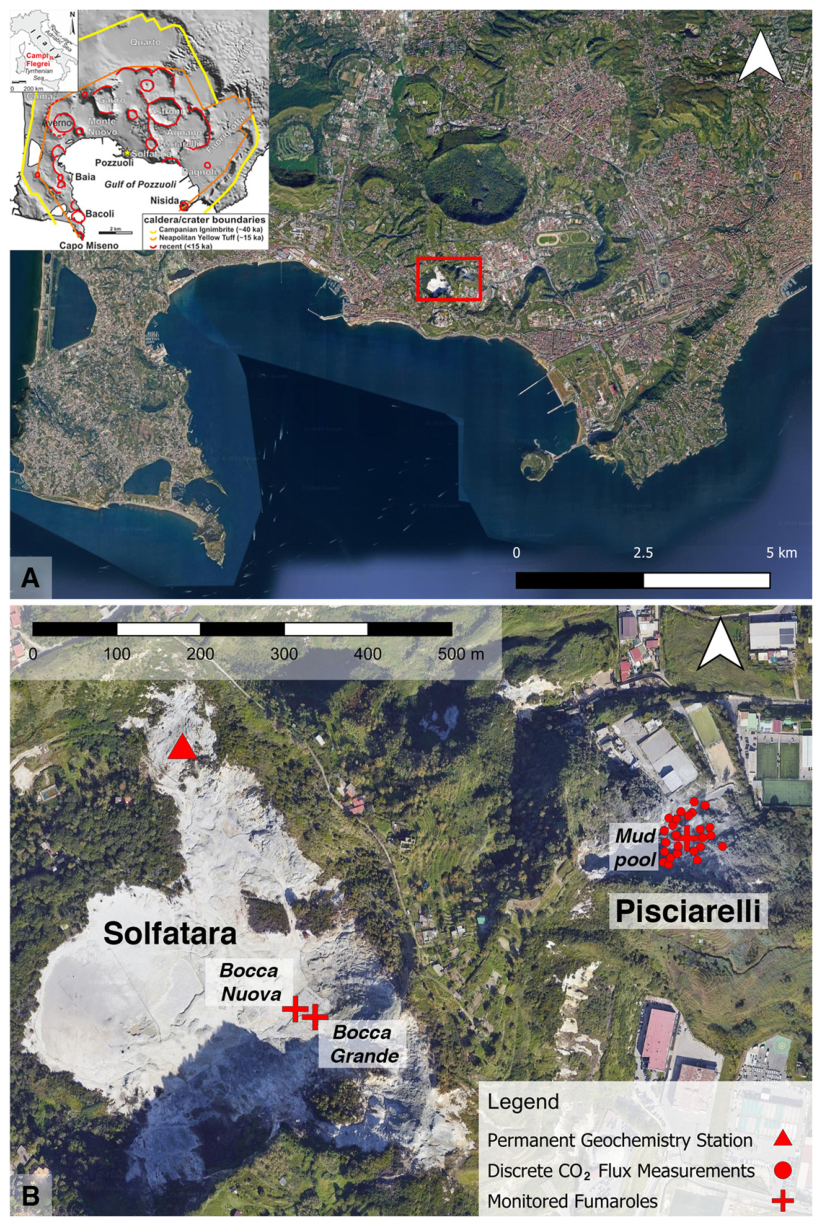
Understanding how and when critical transitions occur in volcanic systems is a fundamental challenge in Earth sciences. These systems are shaped by nonlinear and multivariable interactions between geological, geophysical, and geochemical processes that evolve dynamically over time. Anticipating changes in their behaviour requires both continuous multidisciplinary monitoring and analytical frameworks capable of identifying subtle interdependencies. The Solfatara–Pisciarelli (SP) fumarolic area, located within the Campi Flegrei caldera (CFc) in Southern Italy, provides an exceptional natural laboratory in which to investigate these dynamics [1] (Figure 1).
The CFc is a large resurgent caldera formed by two major explosive eruptions—the Campanian Ignimbrite (~39 ka) and the Neapolitan Yellow Tuff (~15 ka) [2,3]—that has experienced repeated unrest episodes marked by ground deformation, seismicity, and gas anomalies. The SP area, northeast of the town of Pozzuoli, is among the most active sectors of the caldera [4]. It is characterized by intense hydrothermal activity, persistent degassing, and episodic seismic swarms, reflecting the complex coupling between deep magmatic sources and a shallow hydrothermal system [5].
Geophysical and geological studies have revealed that the SP region overlies a diatreme-like structure extending ~3 km below the surface, composed of highly fractured volcanic rocks and fault systems that channel deep fluids toward the surface [5,6,7]. Electrical resistivity tomography, magnetotelluric imaging, and 4D seismic tomography have confirmed the presence of fluid-saturated, high-permeability zones and documented dynamic changes in the caldera’s plumbing system during unrest phases [8,9,10]. These structures play a critical role in controlling fluid migration and pressure redistribution, making the area particularly sensitive to magmatic or hydrothermal perturbations.
The interaction between magmatic degassing and hydrothermal circulation also manifests in geochemical variations. Parameters such as CO2 flux, CO/CO2 and CO2/H2O ratios, and equilibrium temperatures and pressures of the hydrothermal system have shown temporal correlations with deformation and seismicity, offering key insights into the system’s evolution [11,12,13,14]. Notably, an increase in fumarolic sulfur emissions since 2018 further suggests a reorganization of fluid pathways and magmatic inputs [15]. Gas fluxes reaching tens of thousands of tons per day, and the coexistence of superheated steam and liquid water in the shallow reservoir, underscore the intense energy exchange occurring at depth [16,17,18].
Between 2018 and 2024, a comprehensive monitoring effort captured high-resolution time series of key parameters, including vertical ground deformation [19,20,21,22,23], seismicity [24,25], surface temperature from UAV and satellite platforms [26,27], and gas compositions and fluxes. This rich multiparametric dataset provides a unique opportunity to assess how physical and chemical signals co-evolve and potentially signal transitions in the system.
In this study, we address the need for an integrated methodology for identifying and quantifying critical transitions in volcanic systems. All analyses were performed on a dataset acquired from this area of intense volcanic activity, as monitored by the multiparametric surveillance system of the INGV—Osservatorio Vesuviano. We employ a novel framework that integrates Multivariable Fractional Polynomial Analysis (MFPA) [28] and Global Critical Point Analysis (GCPA) [29]. MFPA enables the modelling of nonlinear relationships among variables such as ground deformation, seismicity, heat flow, and CO2 flux while incorporating time lags that capture delayed cause-effect interactions. MFPA and GCPA were used as complementary components of the analytical framework. MFPA quantified lagged and interpretable associations with ground deformation, whereas GCPA applied quadratic optimization to a representative set of non-collinear and temporally coherent time series to identify temporal breakpoints across the monitored system, without relying on thresholds or the prediction of specific events.
Our aim is to identify systemic changes in the SP hydrothermal–magmatic complex by detecting associations between key parameters and their temporal structures. By uncovering lagged, nonlinear relationships and pinpointing critical transitions, this approach enhances our capacity to interpret volcanic unrest.

2. Materials and Methods

The dataset spans 2018–2024 and consists of high-resolution time series of key geophysical and geochemical parameters essential for monitoring the volcanic activity of the SP system. These parameters comprise vertical ground deformation (InSAR), seismicity (from the SERENADE-GOSSIP catalogue), fumarolic CO2 flux, and thermal data acquired through UAV-based infrared imaging. Additional geochemical parameters—such as CO concentration, CO/CO2 and CO2/H2O ratios, as well as equilibrium pressure and temperature—were obtained from a combination of automatic monitoring stations and monthly laboratory analyses conducted by INGV–Osservatorio Vesuviano.
The monitoring focuses on the main active degassing vents: Bocca Grande (BG) and Bocca Nuova (BN) at Solfatara, and the Pisciarelli mud pool fumaroles, located less than 300 m away on the external eastern flank of the Solfatara crater (Figure 1B). Due to the close spatial proximity and the consistent geochemical and physical behaviour observed across these sites—such as similar gas compositions, temperature trends, and fumarolic dynamics—these areas are treated as a unified hydrothermal–magmatic system. This interpretation is supported by previous studies [8,30,31] which highlight the common origin and interconnected behaviour of the two fumarolic fields. Accordingly, in this study, the Solfatara and Pisciarelli fields are collectively referred to as the SP system.
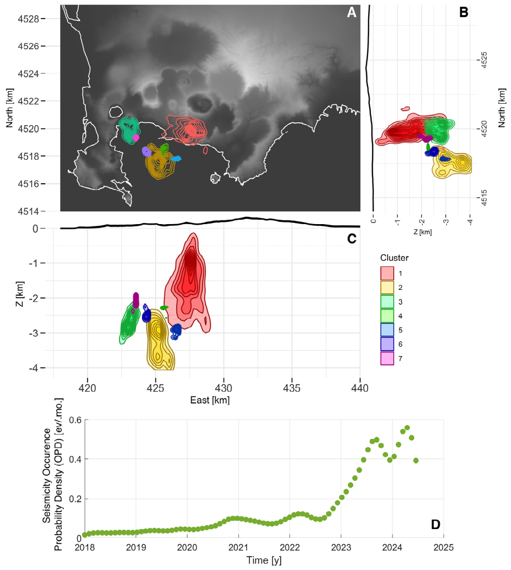
To improve the spatial characterization of the seismicity and its temporal evolution, a clustering analysis was applied to the SERENADE-GOSSIP earthquake catalogue using the DBSCAN algorithm [32,33]. This density-based method identifies spatially coherent groups of seismic events and allows for the discrimination between background activity and structurally significant clusters. The analysis revealed a dominant vertical structure (Cluster 1), located beneath the Solfatara–Pisciarelli area, which is interpreted as a persistent fluid and/or fracture conduit related to the active hydrothermal system. Additional minor clusters were detected across the wider caldera, associated with transient or localized swarm-like activity. The identification of Cluster 1 was instrumental in isolating the subset of events most relevant to the SP system and in enhancing the temporal resolution of the multiparametric analysis.
All time series were preprocessed to facilitate cross-comparison and integration into the multivariate statistical models presented in the following sections. This section is organized in two parts: the first describes the sampling procedures and acquisition protocols for each dataset—including sensor specifications, thermal clustering methods, DBSCAN parameters, and data preprocessing steps—while the second presents the resulting time series for each parameter. Following the data collection and in Appendix A their description.

2.1. Data Collection

2.1.1. Fumarolic Gas Composition (Bocca Grande—BG, Solfatara)

The compositional data used in this study were collected monthly from Bocca Grande (BG), the main fumarolic vent at La Solfatara, using an automatic sampling station. Gas samples were analysed for chemical composition at the Geochemistry Laboratory of INGV-Osservatorio Vesuviano (Figure 2). Samples were collected in under-vacuum flasks containing 4N NaOH solution [34,35] and analysed for major gas species. Analytical procedures followed [36], using gas chromatography with a single injection on dual molecular sieve columns (MS 5 Å capillary, 30 m × 0.53 mm × 50 μm) with TCD detectors and He/Ar as carrier gases. CO2 absorbed in the alkaline solution was oxidized with H2O2 and quantified by acid–base titration. CO was measured in dry gas samples using a water-cooled condenser (20–30 °C), chromatographic separation on a MS 5 Å 1/8 × 50 in column (He carrier), and detection with a high-sensitivity Reduced Gas Detector (HgO).

2.1.2. CO2 Flux and Thermal Anomalies (Pisciarelli Site)

CO2 emissions at the Pisciarelli fumarolic field were continuously monitored from 1 December 2018 to 30 May 2024, with daily resolution and point-based spatial data (Figure 2).
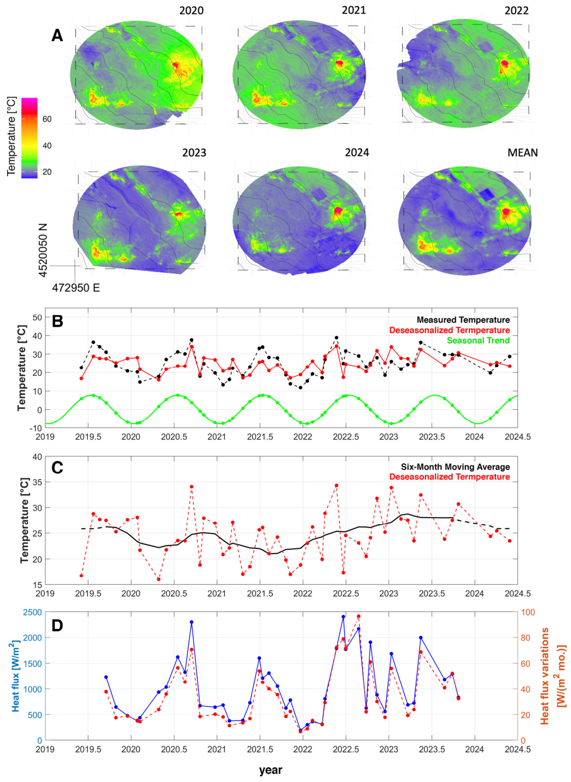
Thermal surveys were carried out monthly from September 2019 to October 2023, with additional surveys up to May 2024 (Figure 3). UAV-based radiometric thermal imaging was conducted during nighttime or evening hours to minimize solar interference. About 50 thermal mosaics were generated from flights at altitudes between 55 and 70 m a.g.l. [26], with some mosaics combining data from different flight plans. Thermal mosaics were processed using the method of [37] to delineate surface thermal anomalies and quantify emitted thermal energy. Clustering algorithms [DBSCAN and k-means; 32, 33] were applied to segment images into thermally homogeneous areas. Each cluster was annotated with temporal metadata and thermal attributes (e.g., average temperature, thermal flux, size in pixels and m2), then reanalysed with DBSCAN to track temporal evolution. Full details of data acquisition and processing are reported in [26].

2.1.3. Seismicity (GOSSIP/SERENADE Catalogue)

Seismic data were sourced from the SERENADE database [38,39] via the GOSSIP portal [40], which provides hypocentral parameters, magnitude (Md), and station arrival times (Figure 4). Hypocenter locations were calculated using the Hypo71 code [41] with local 1D velocity models for Vesuvius, Campi Flegrei, Ischia, and surrounding regions. The database integrates automatic Earthworm-based solutions [42] and manual revisions by the INGV-OV Monitoring Room and Seismic Laboratory. Static event pages are generated with the Serewrap software version 5.3.2 [43], triggered with each new event insertion via the WESSEL portal [39,44].
Seismic events from 2018 to May 2024 with Md ≥ 0.2 were extracted and spatially filtered within a 1000 m buffer around the target area.

2.1.4. Ground Deformation (Sentinel-1 InSAR Analysis)

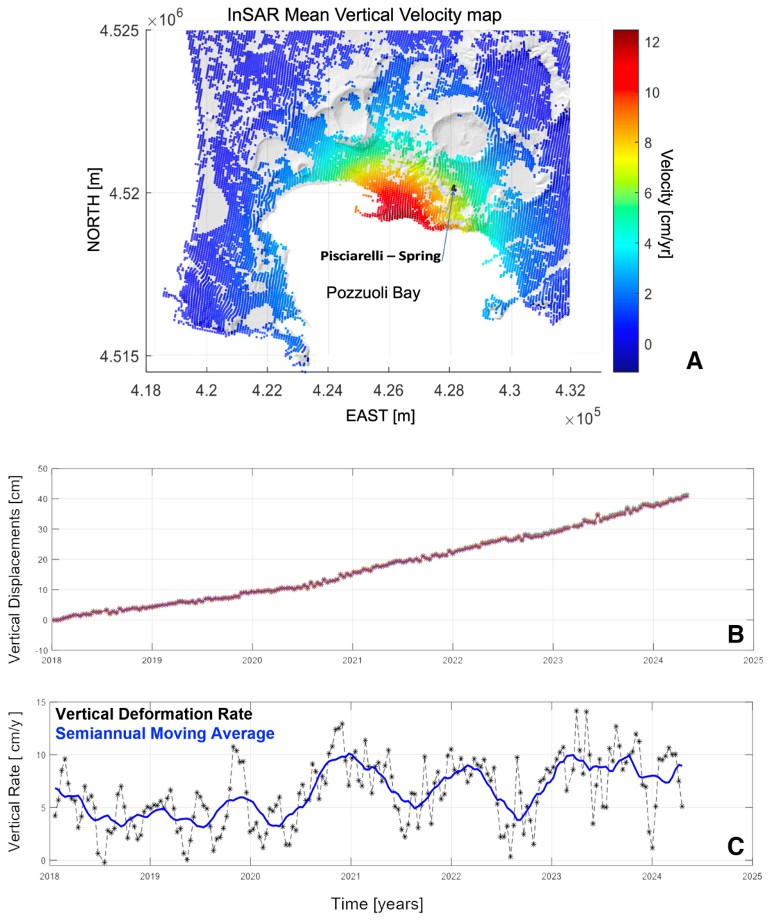
Ground deformation data were derived from Sentinel-1A (S1-A) C-band SAR images (λ = 5.54 cm) acquired in Interferometric Wide mode (IW) from January 2018 to April 2024, along ascending (Path 44) and descending (Path 22) orbits, each with 191 images (Figure 5). The Small Baseline Subset (SBAS) multi-temporal DInSAR method [45,46,47] was applied independently to both tracks. A total of 2101 interferograms were generated per track, with a maximum temporal baseline of 144 days. Interferograms were flattened using precise orbits and the NASA SRTM 1-arc-second DEM (https://dwtkns.com/srtm30m; accessed on 13 December 2024). Ascending and descending LOS displacements were combined [48,49] to obtain vertical and horizontal deformation maps, geocoded and referenced to a stable point. The final dataset achieved cm-to-mm accuracy [22], with a spatial resolution of ~90 m and a ~12-day temporal resolution, totalling 191 layers. Vertical deformation was determined as the average value (or mean) of the time series of the four closest pixels to the target area, selected within a 100-m radius.

2.2. Data Processing and Methods

2.2.1. Multivariable Fractional Polynomial Analysis (MFPA)

The primary objective of this study was to investigate the association between the temporal behaviour of deformation, seismic activity, and specific physical and chemical factors. This goal, along with the characteristics of the available dataset, guided the selection of specific statistical procedures and analytical approaches.
The datasets were initially processed to ensure comparability across variables with different units and scales. The multiparametric dataset was resampled to a common 1/10 of a year time step to allow comparisons across variables with different temporal resolutions. Specifically, the continuous daily CO2 flux data were aggregated by computing monthly means, the seismicity is considered the monthly occurrence of events, the 12-day InSAR deformation data were interpolated to the same 1/10 of a year grid using a spline-based method, and the monthly thermal and gas data were retained as originally measured. This resampling ensured consistency among datasets, minimized artefacts due to mismatched sampling rates, and provided a balanced compromise between the coarsest and the most frequent observations. Validation analyses confirm that the resampled deformation series remain highly correlated (R2 > 0.95) with the original 12-day data, indicating that no significant information was lost.
A multivariable regression model was employed to assess the association between our main variable of interest (vertical ground deformation) and the set of measured physical parameters. The aim is to identify statistically significant correlation for each variable, independent of other factors.
Vertical ground deformation was selected as the dependent variable because it represents one of the most robust, consistently monitored, and informative indicators of unrest at Campi Flegrei. It reflects pressure variations in the magmatic–hydrothermal system and provides a reliable benchmark against which the explanatory power of other geochemical and geophysical variables can be tested.
Since the data are structured as a single-point time series across multiple variables, we adopted an autoregressive model. In this approach, a lagged value of the dependent variable was included as an additional explanatory factor.
The optimal lag order—that is, the number of periods considered backward in time—was determined by the concordance of four information criteria together with a sequence of likelihood ratio (LR) tests. Specifically, we relied on Akaike’s Final Prediction Error Criterion (FPE), the Akaike Information Criterion (AIC), the Hannan–Quinn Information Criterion (HQIC), and the Schwarz Bayesian Information Criterion (SBIC). All tests were performed using Stata’s varsoc command.
As reported in Table 1, all five tests indicated the first lag as the optimal choice. This decision is also consistent with the principle of parsimony, which should guide model selection, as it enhances interpretability, reduces model complexity, and limits the risk of multicollinearity.
The use of an autoregressive specification was justified by two main considerations.
First, from a technical standpoint, it mitigates the statistical bias caused by temporal dependence of the dependent variable. If, in standard regression models, observations of the dependent variable are not independent but temporally correlated, can inflate variance estimates if left unaddressed. By contrast, the autoregressive model explicitly accounts for this temporal dependence, thereby stabilizing the estimates of other covariates and allowing for more accurate inference.
Second, the inclusion of a lagged dependent variable as a regressor helps absorb unmeasured influences that affect the dependent variable, thus capturing residual dynamics otherwise left unexplained [50].
Therefore, when the focus—as in our case—is on the covariates included in the model and their relative impact on the dependent variable, comparing specifications with and without the lagged dependent variable can help disentangle and more accurately quantify the contribution of each covariate.
Because deformation is a strongly persistent temporal process, the first lag of deformation was included to account for serial dependence and to define the structurally appropriate reference model for inference. In this setting, the global R2 of the lagged model was considered only as a measure of overall fit and not as a direct indicator of the explanatory role of the external predictors. The contribution of seismic, thermal and geochemical variables was instead evaluated through their partial R2 within the full lagged model, i.e., as the fraction of explained variance attributable to each predictor after accounting for the autoregressive component and the other retained covariates. In addition, the robustness of variable selection was assessed through bootstrap inclusion frequency (BIF), so that the relevance of external predictors was interpreted jointly in terms of explanatory contribution and selection stability. The model without lag was retained only as a comparative analysis, useful to assess how omission of temporal dependence affects variable selection and the redistribution of explained variance across predictors.
In other words, by acting as a proxy for unobserved factors influencing the dependent variable, the first lag absorbs unmeasured effects, thereby stabilizing the estimates of the independent contributions of other covariates and enabling a more accurate evaluation.
The identification of the best final model followed the pragmatic approach suggested by [28], summarized as follows:
  • Selection of the final model by including factors significantly associated with the dependent variable, while assessing the functional form (linearity/non-linearity) of continuous factors using the multivariable fractional polynomial (MFP) algorithm.
  • Evaluation of the overall and individual contribution of the factors selected in the final model to the dependent variable by calculating both the global variance explained (R2) and the individual variance partition for each significant factor (R2p). The Shapley-Owen decomposition algorithm [51] was used to partition global R2, quantifying each variable’s impact independently of others, i.e., the impact with all other factors held constant.
All models were checked for multicollinearity by calculating the Variance Inflation Factor (VIF) for each variable in the final model. A VIF value greater than 5 was considered indicative of multicollinearity [52,53].
The internal validity of models was computed by assessing the stability of each model characteristics using non-parametric bootstrap sampling [28]. Given the coefficients estimated with the regression model, using the described model-building procedure, the stability of each factor tested in the model was measured by the frequency at which this factor was selected as “significant” in a large series (1000) of bootstrap replications of the dataset by applying the same procedure. Each bootstrapped dataset may be considered a random replicate of the original dataset; thus, the BIF of a given factor in the final model quantifies the confidence we can place on its association with the outcome (stability), considering the expected random variability of the data.
To visualize the relationship between a dependent variable and a specific independent factor controlling for other significant variables in the final model, a scatterplot was created. In this plot, the dependent variable values were adjusted with respect to the mean of other significant variables considered in the model. Specifically, the relationship between y and one of the x variables was illustrated by adjusting observed y values for each item according to deviation of other observed x variables from their respective means, using estimated coefficients. Data were analyzed using Stata version 18.0 (StataCorp LP, College Station, TX, USA), using the following commands: estat ic, estat vif, mfpa, mfpboot, regress, shapleyx, varsoc. Statistical significance was set at p ≤ 0.05 for univariate comparisons, variable selection, and testing between variable transformations within the MFP procedure.
The MFPA was used to identify interpretable lagged associations with deformation and to exclude collinear observables, thereby defining a parsimonious set of non-redundant candidate variables. A representative subset of these temporally coherent and physically complementary time series was then considered in the subsequent Global Critical Point Analysis to identify meaningful transitions in the time domain. The MFPA model converged in fewer than 30 iterations per run, with an average computation time below 1 min on standard desktop hardware (Intel i7 processor, 16 GB RAM). This performance confirms the suitability of the approach for potential near-real-time implementations in operational monitoring environments.

2.2.2. Global Critical Point Analysis (GCPA)

The GCPA method is used to identify significant temporal transitions in multiparametric datasets by detecting the time at which the system exhibits the maximum collective deviation from background behaviour. It leverages Quadratic Programming (QP) [54] to identify a critical time index corresponding to the maximum aggregated deviation across all normalized variables. This critical point may correspond to a phase where the system transitions from stability to chaos or shifts between different equilibrium states. In the context of the SP system, GCPA serves as a valuable tool for analysing variations in geophysical and geochemical parameters, helping to detect potential systemic changes without aiming to predict specific events, such as an eruption. Instead, the methodology focuses on understanding the system’s evolution and identifying precursors to critical transitions, essential in volcanic systems where gradual or subtle changes may indicate an approaching tipping point (global critical point). The GCPA statistical technique identifies the temporal moment when significant changes occur across multiple variables simultaneously. These variables include physical or chemical parameters recorded over time, such as ground deformation rate, seismicity, temperature, heat flow, and CO2 flux. By pinpointing a single temporal moment representing overall change across all analysed time series, GCPA simplifies the complexity of multiparametric analysis and identifies a common breaking point explaining observed variations. Moreover, the application of quadratic optimization using the Karmarkar method [55] has improved the efficiency of global critical point detection, allowing for a more precise assessment of systemic changes. This optimization framework enhances the reliability of transition detection by providing a mathematical basis for identifying system shifts beyond simple threshold-based analyses. The analysis was performed using R software version 4.4.1 [56] and involved five main steps:
  • Data Preprocessing and Normalization: input time series are normalized to standardize datasets with different units or scales, (e.g., temperature, seismicity, gas flux), ensuring meaningful and robust comparison of variables while reducing the risk of bias in subsequent analysis.
  • QP for Critical Point Identification: the problem is modelled using a quadratic objective function that maximizes deviations from expected or average behaviour. The matrix Q is defined as the identity matrix, ensuring independence between temporal indices and guaranteeing convexity of the optimization problem, while the vector c is defined as the aggregated absolute deviation across all normalized variables at each time step, such that: c t = i = 1 N z i ( t ) . The negative sign ensures that minimizing the objective function is equivalent to maximizing the collective deviation from background conditions. Temporal constraints are applied to ensure that the identified critical point lies within the observed data range, preventing the selection of spurious points.
    To formally identify the time of critical transition, we structured the analysis as a QP optimization problem. Specifically, the critical point was defined as the time index minimizing the following objective function:
    f x = 1 2 · x T · Q · x + c T · x
    which represents a quadratic function in matrix form, commonly used in quadratic optimization (QP); where x R n is a one-hot encoded vector (i.e., a binary vector with a single non-zero entry), selecting a unique temporal index (with 1 at the candidate critical time and 0 elsewhere), and c R is a column vector of linear coefficients collecting the normalized mean deviation of each parameter over time. More specifically, Equation (1) is a typical objective function in quadratic optimization problems, where 1 2 · x T · Q · x is the quadratic term and represents a paraboloid if QQ is positive definite, and c T · x is the linear term.
    Note that the factor 1/2 is conventional and useful because the derivative of the quadratic term is Q · x which simplifies the gradient computation:
    f x = Q · x + c
    Given the one-hot constraint on x , the optimization problem is equivalent to evaluating the objective function across all candidate time indices and selecting the time corresponding to the minimum value.
    Finally, we remark that the matrix Q encodes the co-evolution and coupling between variables (e.g., deformation, seismicity, gas), while c provides a temporal profile of their joint anomalies. This formulation allows us to detect the time step where the system collectively exhibits the greatest deviation from background behaviour, provided that this deviation exceeds the variability expected under stationarity conditions, as assessed through a Moving Block Bootstrap (MBB) procedure.
    To assess the statistical robustness of the detected critical point, a Moving Block Bootstrap (MBB) approach is implemented to preserve temporal dependencies within the time series. Many bootstrap resamples are generated, and the distribution of detected critical points is analysed. The mode of the distribution is used as the most representative estimate, while confidence intervals (e.g., 5th–95th percentile) are computed to quantify uncertainty. In the absence of such evidence, no critical point is identified. Moreover, we stress that this identification is retrospective, as an ex-post characterization of past dynamics rather than as a predictive tool.
  • Optimization Techniques: the R Optimization Infrastructure (ROI) package [57], combined with the ROI.plugin.quadprog plugin, is used to solve the QP problem. This setup efficiently handles large datasets with multiple parameters and integrates advanced optimization techniques, including:
    • Interior-Point Methods: ensure convergence by iteratively refining the solution within the feasible region.
    • Conjugate Gradient Methods: particularly suitable for large and sparse datasets.
    • Penalty and Barrier Methods: facilitate constraint handling and enhance computational efficiency.
  • Critical Point Detection: the critical point corresponds to the time index that minimizes the objective function, i.e., maximizes the aggregated deviation across all variables, representing the moment when significant transitions occur across the analysed parameters [58].
  • Visualization and Interpretation: the identified critical point is visualized within the context of normalized time series using the ggplot2 package [59]. In addition, we used the Shapley decomposition algorithm to identify the partitioned contribution of each time series to detect the CPs.
The GCPA method is particularly suited to complex systems with dynamic and interdependent parameters. By integrating representative, non-collinear geophysical and geochemical variables, such as ground deformation, seismicity, temperature, heat flow, and CO2 flux, the algorithm identifies moments of significant systemic change. These insights are crucial for understanding volcanic behaviour, assessing hazards, and refining monitoring strategies. The GCPA framework is adaptable to large datasets and diverse scientific applications, allowing the incorporation of various constraints and objective functions tailored to specific research needs. For our analysis, GCPA was applied to a representative subset of non-collinear, temporally coherent time series. MFPA contributed to this selection by excluding collinear observables and by providing an interpretable benchmark for variable screening, but not as a strict sequential filter. To evaluate the method’s response and its robustness to variations in multiparametric time series, we performed two analyses by considering different observation intervals for the parameters: the first (2018–2023) that represents a subset of the second (2018–2024).
It is important to highlight that the GCPA method does not impose the existence of a critical point and identifies one only when a statistically robust collective deviation from stationarity is observed.

3. Results

We applied MFPA to determine the best combination of geophysical and geochemical parameters that explain ground deformation at the SP site, considered the dependent variable. This choice is motivated by the prominent role that vertical ground deformation plays in signalling pressurization processes at the Campi Flegrei caldera. Long-term geodetic observations have consistently linked episodes of uplift to periods of increased hydrothermal or magmatic activity [22,60,61]. In the Solfatara–Pisciarelli area, deformation is often the first measurable indicator of subsurface changes, and it integrates complex interactions such as gas accumulation, heat transfer, and fluid migration. Therefore, it provides an effective dependent variable for exploring multiparametric cause-effect relationships in the SP system. Importantly, the regression framework does not aim to diminish the central role of deformation, but rather to investigate how other observables contribute to explaining its variability and to highlight potential coupling mechanisms. In addition, deformation is measured with high spatial and temporal resolution via InSAR techniques, ensuring the reliability and continuity required for regression-based analyses. This makes it a valuable proxy for unrest modelling when combined with complementary parameters such as CO2 flux, seismicity, and heat flow, without implying predictive capability in the sense of forecasting. The goal was to capture significant nonlinear associations and delayed effects that influence vertical deformation dynamics, offering a robust interpretation of the physical mechanisms behind observed surface displacements. Following the assessment of multicollinearity among all parameters (geochemical parameters: T(CO–CO2) [°C], CO [µmol/mol], CO/CO2, CO2/H2O, CO2/CH4, P(CO–CO2–H2–H2O) [bar] and CO2 flux; land surface temperature; heat flux and seismicity), only those showing no collinearity were included in the MFPA. We developed two regression models: one incorporating a time-lag structure (LAG model) and one without (NO-LAG model). In the LAG model, the dependent variable (vertical ground deformation) is regressed against its own past value (i.e., the value observed 1/10 of a year earlier), in addition to other explanatory variables.
Table 2 should be interpreted with the lagged model as the primary inferential specification, since it accounts for temporal dependence in deformation, whereas the unlagged model is shown for comparative purposes only. Table 2 summarizes the coefficients, explained variance, and model selection metrics for both approaches. In the LAG model (Panel A), the main retained contributors were the first lag of deformation, seismicity, and P(CO–CO2–H2–H2O), whereas the other covariates did not show significant independent associations within the final specification.
The near-unity global R2 (0.999) is consistent with the strong persistence of the deformation series, but it should not be interpreted as implying that the external covariates alone explain nearly all the observed variability. Rather, within the lagged model, the relative contribution of the retained predictors was quantified through their partial R2, showing that the explained variance was shared between the autoregressive component and the selected external covariates (44,4% of the first versus the joint 55.6% of the 2 significant covariates). This interpretation was reinforced by the bootstrap inclusion frequency analysis, which showed high selection stability for seismicity and P(CO–CO2–H2–H2O), supporting their role as the most robust external contributors once temporal dependence had been accounted for.
It is important to notice that the other covariates, even if in the final models are not significant, show a relatively high BIF, especially for heat flow (21%), the CO2/H2O ratio (49.5%) and CO2 flux (47.6%). The Akaike Information Criterion (AIC = −24) further supports the model’s parsimony and goodness of fit.
By contrast, the unlagged model (Panel B), although still yielding a high global R2 (0.97), identified a broader set of apparently relevant external predictors. However, beyond seismicity and P(CO–CO2–H2–H2O), the additional predictors that emerged in this model—temperature, heat flow, and CO2 flow—displayed relatively small partial R2 values (3.9%, 8.9%, and 7.6%, respectively). Thus, omission of temporal dependence did not reveal additional major associations but rather redistributed a limited fraction of explained variance toward secondary predictors, while enlarging their apparent role.
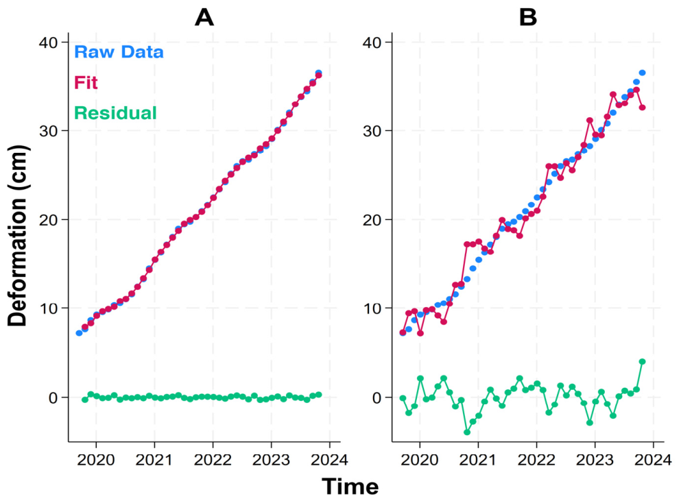
Figure 6A displays the observed deformation time series (blue dots) overlaid with the LAG model prediction (red line), showing excellent agreement. The residuals (green dots) are minimal and randomly distributed. In contrast, the NO-LAG model (Figure 6B) resulted in increased residuals, lower explanatory power (R2 = 0.97), and significantly higher AIC (165.3) values.
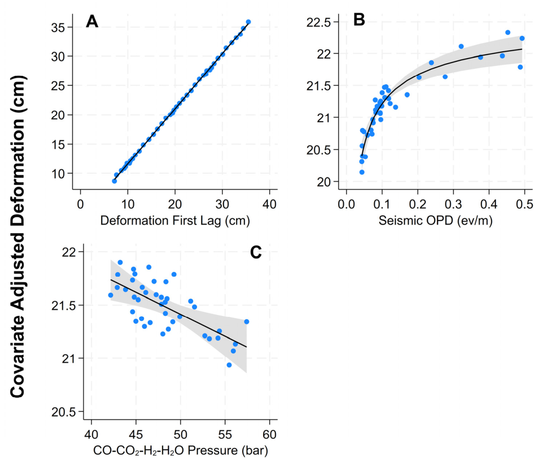
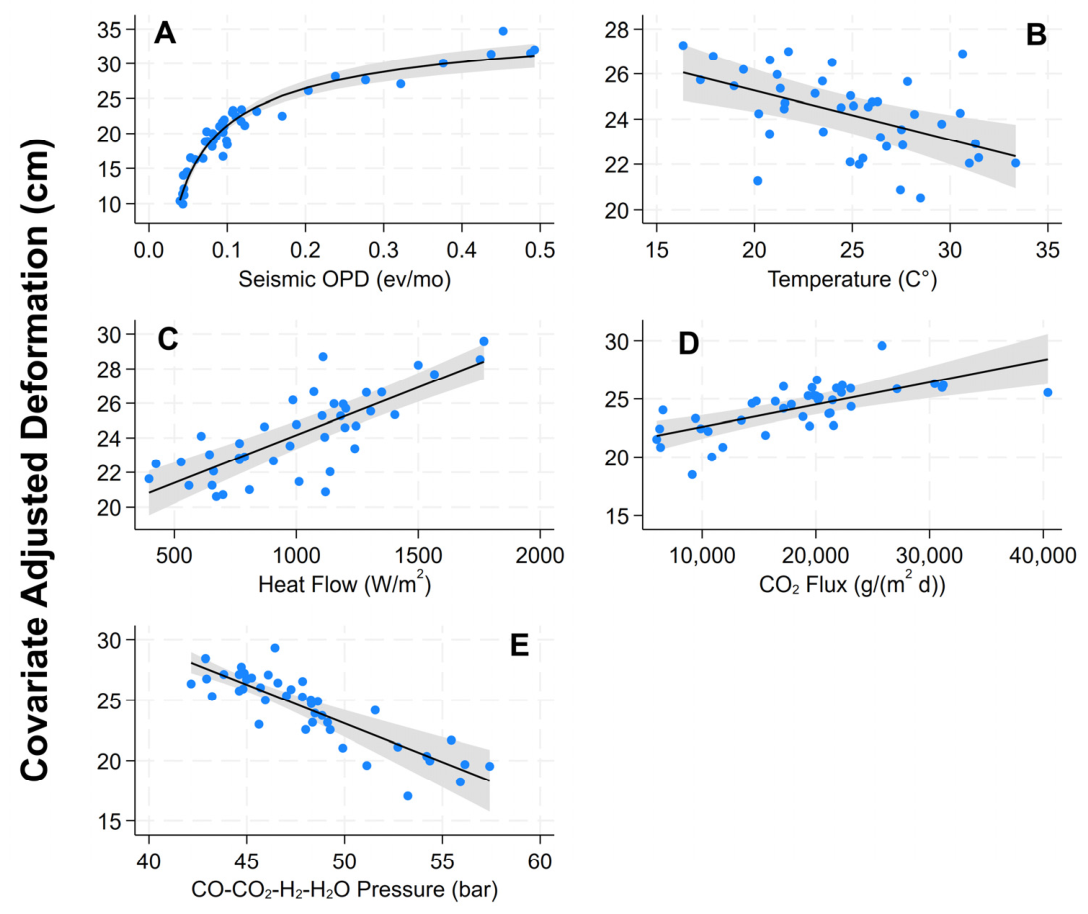
Covariate-adjusted partial relationships (Figure 7) revealed a strong positive linear association for the first-lag deformation (Figure 7A), a positive non-linear relationship for seismicity (Figure 7B) and negative linear association for equilibrium pressure of hydrothermal system (Figure 7C).
Figure 8 illustrates nonlinear relationships and inverted trends among the five most relevant predictors. Despite strong individual contributions, the NO-LAG model underperformed relative to the LAG model across all evaluation metrics.
The MFPA results informed, but did not rigidly determine, the subsequent Global Critical Point Analysis (GCPA). For the GCPA, we selected a representative subset of non-collinear and temporally coherent observables capturing complementary components of the SP system, rather than restricting the analysis to the statistically significant covariates of a single regression specification. In this way, MFPA and GCPA addressed different but complementary questions: the former quantified lagged associations with deformation, whereas the latter investigated the collective temporal reorganization of the monitored system. While the MFPA approach treats ground deformation as the primary dependent variable, the GCPA treats the entire dataset as a set of interdependent time series. This allows for the identification of critical points by analysing the collective behaviour of the parameters in their original temporal sequence, moving beyond the functional relationships modelled in the previous step.
The analysis was performed over two overlapping time windows: 2018–2023 and 2018–2024. The first interval was selected to identify transitional behaviours prior to the onset of the 2023 critical point (CP2), while the extended window allows for the detection of the additional system-wide reorganization that characterizes CP2. This approach supports a robust validation of the Global Critical Point Analysis (GCPA) framework across different temporal baselines.
When extending the observation window, GCPA identifies the dominant systemic transition rather than all local maxima. CP1 remains a valid transition, but CP2 represents a larger and more coherent multiparametric reorganization that becomes dominant when the full 2018–2024 interval is considered.
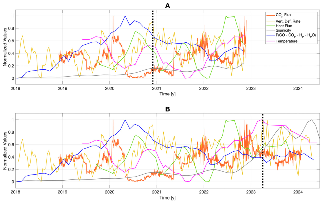
We applied Global Critical Point Analysis (GCPA) to six normalized series (deformation rate, seismicity, temperature, heat flux, CO2 flux, P(CO–CO2–H2–H2O)), selected as a non-collinear and physically complementary subset of the monitored observables, identifying two distinct systemic reorganizations: CP1 (30 November 2020) and CP2 (1 April 2023). In this respect, MFPA contributed to the screening phase by identifying collinear variables to be excluded and by providing an interpretable reference framework, whereas GCPA was used to investigate the joint temporal behaviour of the retained system-level signals. In addition, deformation was introduced in GCPA as deformation rate rather than cumulative vertical displacement, because the latter is nearly monotonic over the observation window and would be less informative for detecting temporal reorganizations of the system.
The normalized time series (Figure 9) show clear regime shifts. Near CP1 (30 November 2020; Figure 9A), peak anomalies appear in deformation rate, temperature, and seismicity, with concurrent increases in in CO2 flux and a similar behaviour for P(CO–CO2–H2–H2O) and heat flow; towards CP2 (1 April 2023; Figure 9A), there are coeval peaks in deformation rate and thermal signals, while there are also changes in their slope for seismicity and degassing signals (Figure 9B), consistent with a more open, connected system.
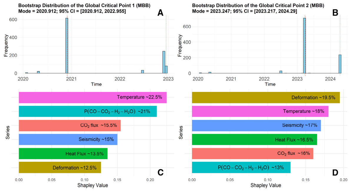
Block-bootstrap (MBB; Figure 10) yields sharp modal distributions with asymmetric 95% CIs (CP1: 2020.912 [2020.912, 2022.955]; CP2: 2023.247 [2023.220, 2024.290]; Figure 10A,C).
Shapley decomposition quantifies transition structure: CP1 is thermal–chemical (≈Temperature, 22.5%; P(CO–CO2–H2–H2O) content, 21.0%; CO2 flux, 15.5%; Seismicity, 15%; Heat flow, 13.5%; Deformation rate, 12.5%; Figure 10B), while CP2 is balanced multiparametric (≈Deformation 19.5%, Temperature 18%, Seismicity 17%, Heat flow 16.5%, CO2 16%, P(CO–CO2–H2–H2O) 13%; Figure 10D).

4. Discussion

The proposed methodology allows us to reveal a strong overall association between the variables of interest and the set of factors tested in the models. Specifically, regarding ground deformation, seismic activity plays a significant role, accounting for one-third of the overall variance even when a lag term is included in the model. In other words, it explains a substantial portion of the variance while also accounting for unmeasured associative factors. This evidence is further supported by the high stability of seismic activity in the final models, as indicated by its consistently high frequency of statistical significance (BIF above 97%, Table 2) in the bootstrapped datasets. In models without the LAG term, other factors gain prominence in the association, attempting to compensate for the unmeasured influences. The high BIF values, observed for almost all variables in these models, reflect this compensatory effect. In particular, for a substantial number of factors, except seismic activity, we observed non-significant levels paired with high BIF values, and vice versa. This suggests that none of these factors, aside from seismic activity, establishes a stable association.
The LAG model effectively mitigates the statistical bias caused by the temporal dependence of the dependent variable. It demonstrates a strong correspondence between observed data (“Raw data”) and the model fit (“Fit”), with residuals (“Residual”) remaining close to zero (Figure 6A). This indicates that the model successfully absorbs unmeasured influences that affect the dependent variable, thus capturing residual dynamics that would otherwise remain unexplained. I The comparison between lagged and unlagged specifications should therefore not be read as a direct estimate of the contribution of the lag term from differences in global R2. Rather, it highlights the fact that omission of temporal dependence may inflate the apparent role of external covariates by forcing them to absorb part of the autoregressive structure of the deformation process. This interpretation is supported not only by the redistribution of partial R2, but also by the bootstrap inclusion frequency results. In the lagged model, the main external associations were those that combined non-negligible explanatory contribution with high selection stability, particularly seismicity and P(CO–CO2–H2–H2O). In the unlagged model, additional predictors became statistically significant, but their individual contribution remained modest, indicating that the absence of the lag term broadens apparent relevance without identifying further major drivers of deformation. For this reason, the lagged model was considered the main inferential framework, whereas the unlagged model was interpreted as a sensitivity analysis.
In contrast, in the NO-LAG model, the residuals exhibit greater variability and a systematic temporal oscillation, suggesting that the model fails to adequately absorb unmeasured effects, thereby stabilizing the estimates of the independent contributions of other covariates.
In a strongly persistent time series, omitting the lagged response does not simply reduce model fit; it changes the allocation of explained variance across predictors and may enlarge the apparent role of external covariates by forcing them to absorb part of the unmodeled temporal dependence.
The near-stationary residuals close to zero in Figure 6A further confirm the model’s effectiveness in capturing these unmeasured effects.
The interpretation of associations between any single covariate and deformation must always be considered under the assumption that the other covariates remain constant (ceteris paribus). Observing the association between seismicity and deformation in both models, LAG and NO-LAG, allows us to better understand the reason for the non-linear relationship. Beyond a certain threshold, the increase in seismic events is not associated with a significant increase in deformation, because the system is already highly fractured. In this scenario, the causes of further uplift are likely to be sought elsewhere, such as in fluid ascent.
Regarding P(CO–CO2–H2–H2O), it effectively represents a pressure capable of opposing lithostatic confinement. The reduction in the partial pressures of volatiles at equilibrium can be interpreted as the result of two main processes leading to contrasting scenarios: (i) a significant reduction in lithostatic loading conditions, associated with ductile–fragile gravitational tectonics phenomena such as volcano spreading [62], which determine lateral mass migration, and (ii) magma buoyancy processes, typical of the resurgent caldera scenario, which involve a direct upward overpressure due to the migration of fluids through the highly fractured intra-caldera lithological units, resulting in a net release of gaseous volumes.
In the specific case of Campi Flegrei, geodetic observations over the last two decades highlight a progressive uplift of the topographic surface. This behaviour is consistent with a scenario where equilibrium overpressures have favoured the drainage and subsequent release of fluids toward shallower levels, where the trapping of these gases within fractured systems generates the superficial pressure increase responsible for the uplift. The association between deformation and the equilibrium pressure of the gaseous phases therefore outlines a scenario characterised by the coexistence of two concomitant phenomena: (i) a reduction in total equilibrium pressure at the hydrothermal source, due to the drainage of gaseous volumes; and (ii) an increase in ground deformation (uplift), linked to the redistribution and trapping of fluids at shallower levels.
Concerning the NO-LAG model, the significance of nearly all covariates is reasonable, considering that this model must compensate for the 2% difference in total explained variance (R2) compared to the LAG model. Figure 4B illustrates the inverse association between temperature and deformation, holding the other significant covariates in the model constant. By keeping parameters typically linked to mass input, and thus to uplift or positive deformation, such as gas equilibrium pressure and fluxes, constant, the variation in temperature primarily affects the physical properties of the reservoir. This association suggests that the temperature increase is a good predictor of an acceleration of mass and volume loss from the reservoir, leading to subsidence, within a context where the mass input from below is not varying.
It must be remembered that statistical regression methods highlight associative relationships between variables. However, while such associations are a conditio sine qua non for determining causality, the latter requires further physical, geological, and independent observational evidence for confirmation.
Furthermore, the application of the GCPA has been fundamental in identifying the timing and characteristics of critical transitions within the volcanic system. The GCPA method enabled us to detect two major critical points (CP1: 30 November 2020, CP2: 1 April 2023), which correspond to significant variations in multiple monitored parameters, including deformation rates, CO2 flux, and seismicity. These transitions suggest that the SP system underwent two significant evolutionary phases, likely reflecting pressure accumulation and subsequent adjustments within the magmatic-hydrothermal environment.
Overall, the data reveal an evolution from an initial thermal–chemical pressurisation phase (CP1) to an open, balanced regime (CP2). In this later stage, degassing (CO2), mechanical, and thermal processes contribute comparably, a quantitative shift captured by the Shapley weight redistribution and corroborated by time-series analysis. This aggregation process revealed collective behaviours and system-wide responses, such as those leading to CP1 and CP2, that would have been difficult to identify through the analysis of individual variables alone. By emphasising moments of convergence among signals, composite metrics provide a valuable tool for detecting regime shifts in complex volcanic systems. Identifying such transitions is crucial for the objective characterisation of volcanic unrest, as it provides insights into the system’s evolutionary trajectory over time and highlights periods of systemic reorganisation.

4.1. Methodological Advantages over Classical and Non-Parametric Approaches

One of the major strengths of this study is the integration of advanced statistical modelling (MFPA) with critical transition detection (GCPA), providing a novel framework for revealing instability phases in a volcanic system. This approach offers three main advantages:
  • Refined distinction between transient fluctuations and systemic transitions. Applied retrospectively, the methodology allows us to distinguish short-term variations from significant shifts in system dynamics, thereby enhancing the robustness of unrest phase characterisation.
  • Detection of major critical transitions. The identification of two major critical transitions, corresponding to significant changes in the covariates, demonstrates the potential of data-driven approaches for the retrospective characterisation of unrest dynamics, without necessitating the use of deterministic physical models.
  • Potential scalability to other volcanic systems. While our study does not provide proof of generalisability, the methodology offers a testable framework that could be investigated through further case studies and extended to other volcanic systems, particularly complex calderas, to strengthen comparative analytical strategies.
Compared to non-parametric approaches such as decision trees, random forests, or k-nearest neighbours (k-NN), the Multivariable Fractional Polynomial Analysis (MFPA) offers several advantages. First, it allows the identification of interpretable functional relationships between variables, including the assessment of non-linear trends within a parametric framework. This aspect is crucial when the physical meaning of coefficients and lag structures is necessary to relate model output to volcanic processes. Second, MFPA enables the partitioning of explained variance and the decomposition of predictor contributions (via R2p and BIF), providing quantitative insights into which parameters are most strongly associated with the observed dynamics. In contrast, non-parametric methods are often a black box, lacking direct interpretability unless paired with post hoc explainability tools. Third, parametric models are computationally efficient and robust when applied to moderate-sized time series, as in our case, and they require fewer tuning parameters or training iterations. This makes them particularly suitable for high-frequency data streams and for systems where interpretability and parsimony are as critical as descriptive power. Nonetheless, future developments may incorporate ensemble strategies where MFPA is complemented by non-parametric classifiers or anomaly detectors to enhance the sensitivity to rare events and systemic tipping points.
The joint application of GCPA and MFPA represents a significant methodological advancement, as it enables both the identification of non-linear interactions between variables and the detection of critical transitions in volcanic activity. Modelling temporal delays and systemic tipping points is fundamental for understanding the evolution of volcanic unrest and for refining interpretative models of magmatic-hydrothermal systems.

4.2. Link Between Critical Transitions and Overpressure Source

Our results allow us to make a connection between the identified critical transition points (CP1 and CP2) and the evolution of the shallow overpressure source presented by [22], obtained using 4D geodetic tomographic inversion techniques. The GCPA results highlight a distinct critical point corresponding to a major shift in system dynamics, which could be interpreted as a transition from stable conditions to an accelerated phase of potential pressure accumulation and deformation. The temporal coincidence between the GCPA-derived critical point and the inferred migration of the overpressure source proposed by [22] suggests a strong linkage. To their scenario we add information about the thermal and gas behaviour, which is in agreement with their source model. This is supported by the observed increase in CO2 flux and seismic activity recorded prior to their modelled overpressure source migration, as well as by the acceleration in ground deformation patterns detected through InSAR data. Specifically, the increase in CO2 flux, deformation rates, and seismicity, key indicators in the GCPA model, precedes the modelled ascent of pressurized fluids. This supports the hypothesis that the critical point is consistent with the onset of enhanced permeability and fluid mobilisation, potentially facilitating the upward migration of the overpressured magmatic-hydrothermal mixture.

4.3. Applicability and Future Development Perspectives

The integrated MFPA-GCPA framework presented here is not restricted to the Solfatara–Pisciarelli area but can be generalised to other volcanic systems with dense multiparametric monitoring. The core advantage lies in the model’s ability to capture nonlinear and time-delayed interactions between diverse geophysical and geochemical signals, without relying on pre-defined physical thresholds. For example, volcanoes such as Yellowstone, Long Valley, or Taal, where persistent deformation, degassing, and shallow seismicity coexist, could benefit from this approach, particularly in identifying precursory indicators of systemic reorganisation. Similarly, densely monitored stratovolcanoes such as Etna or Stromboli, where cyclic eruptive behaviours are observed, may provide ideal testbeds for implementing time-lagged multivariate models [63,64,65]. We do not claim immediate general applicability of the proposed framework; rather, we present a transferable theoretical methodology whose robustness and scalability would require further evaluation through comparative applications to other volcanic systems to define its actual operational limits.
The case of Campi Flegrei is particularly suited to demonstrate this methodology, due to the exceptional continuity of the time series, the known recurrence of hydrothermal and magmatic transitions, and the availability of high-quality deformation, gas, and seismic datasets. In this context, the proposed framework enhances our ability to recognise critical transitions that may remain hidden in traditional analyses. The accuracy of the identified critical points depends on the resolution and consistency of the input datasets, and uncertainties in model assumptions regarding fluid migration dynamics may affect interpretations. Further validation through independent geophysical and geochemical observations is necessary to refine these findings for identifying and interpreting critical transitions in volcanic systems.
This study demonstrates that the combination of MFPA and GCPA provides an effective tool for understanding the dynamics of complex volcanic systems. The identification of critical transitions in the SP area underscores the potential of this methodology to gain deeper insights into the systemic nature of the volcanic system and its evolution. Furthermore, the introduction of a time-lagged model significantly improves the descriptive power of ground deformation analysis, capturing key interactions between geophysical and geochemical parameters. These insights are particularly relevant for optimising multiparametric monitoring strategies and interpreting the evolution of unrest with greater precision.
In recent years, the identification of precursors to critical transitions in volcanic systems has become a central goal for improving our understanding of system-level dynamics. Several studies have explored this challenge through approaches ranging from tipping point analysis in complex systems to stochastic modelling and machine learning techniques. Indicators of systemic change based on statistical metrics such as increasing variance, lag-1 autocorrelation (critical slow down), and kurtosis have shown promising results in specific case studies on different scientific areas [66,67,68]. However, their application in multiparametric systems is often hindered by high noise sensitivity and limited robustness under complex dynamics [69,70,71]. In comparison, while the integrated MFPA-GCPA framework does not aim at operational forecasting, it presents three key advantages: (i) it explicitly models linear and nonlinear associations between geophysical and geochemical parameters, providing a formalised view of system interdependencies; (ii) it avoids arbitrary thresholds, as critical points are identified through mathematical optimisation over normalised signals, thereby ensuring a more objective detection of regime shifts; and (iii) it enables the temporal integration of multiple signals into a single composite metric, facilitating the detection of systemic transitions rather than isolated events.
Within this perspective, a key prerequisite for further development is the enhancement of both the temporal sampling frequency and the spatial coverage of the monitored covariates. In particular, higher-resolution and more spatially distributed measurements of thermal, geochemical, and flux-related parameters would be necessary to more effectively apply MFPA and GCPA as exploratory tools for identifying changes in the dynamics of volcanic unrest. Such improvements would contribute to a more comprehensive characterisation of the hydrothermal system as a whole, allowing the proposed approach to move beyond the limitations imposed by the current observational framework.
From a methodological standpoint, the framework offers a structured quantitative basis for interpreting the evolution of active volcanic systems. In this sense, the identification of systemic transitions (CP1 and CP2) may offer a formal representation of changes in system behaviour, which could contribute to contextualising the state of the volcanic system and updating interpretative models of unrest. The use of normalised composite metrics may further facilitate the synthesis of complex multiparametric information, potentially improving the clarity and interpretability of data within scientific monitoring platforms [72,73].
The integration of the MFPA-GCPA framework into automated analytical workflows for continuous data streams remains a prospective objective. Achieving this would require not only standardised protocols but also the systematic integration of diverse data streams (e.g., InSAR, seismicity, gas emissions) characterised by adequate temporal continuity and spatial representativeness. Under these conditions, the approach could contribute to the identification of critical phases of unrest, even when surface signals are weak or ambiguous [74]. Finally, while the adaptability of the method suggests possible applicability to different geological settings, its generalisation and potential standardisation within multidisciplinary interpretative frameworks should be approached cautiously and tested through comparative studies across well-instrumented volcanic systems.

5. Conclusions

This study presents a methodological contribution to the study of volcanic unrest, illustrating the potential of a data-driven, multiparametric framework for exploring critical transitions in active volcanic systems. By combining MFPA and GCPA with observational monitoring data, the approach provides a structured basis for improving our understanding of system-level behaviour and its temporal evolution in a complex volcanic environment such as Campi Flegrei over the investigated observational period.
The results indicate that the introduction of a time-lagged model improves the analysis of ground deformation, allowing key interactions between geophysical and geochemical parameters to be captured more effectively. In particular, seismicity emerges as the most stable factor associated with deformation, while the LAG model better absorbs unmeasured influences than the NO-LAG model. The analysis also identified two major critical transitions, CP1 and CP2, which mark important changes in the evolution of the monitored system and support the interpretation of a shift from an initial thermal–chemical pressurisation phase to a more open and balanced regime.
More generally, the integrated MFPA-GCPA framework may represent a useful tool for the retrospective investigation of volcanic unrest, particularly for highlighting nonlinear relationships, time-delayed interactions, and systemic reorganisations that may not be evident when variables are analysed separately. At the same time, the robustness, generality, and practical relevance of the method still need to be further evaluated through enhanced data acquisition strategies, comparative applications to other volcanic systems, and possible future integration into automated analytical architectures. Within these limits, the proposed approach offers a promising basis for advancing the descriptive and interpretative analysis of complex volcanic systems and for supporting the objective characterisation of volcanic unrest dynamics.

Author Contributions

Conceptualization, P.T., A.V. and D.F.V.; methodology, P.T., A.V., D.F.V. and E.M.; investigation, A.B., A.P., S.P., R.A., A.C., P.B., G.A., E.B.S., F.S., R.C., F.M., E.M., F.A. and R.P.; writing—original draft preparation, P.T., A.V., D.F.V., E.M., A.B., R.C., F.S., M.P., S.P., R.P. and E.B.S.; visualization, P.T., A.V., A.B. and M.P.; supervision, P.T., A.V. and E.M. All authors have read and agreed to the published version of the manuscript.

Funding

This research received no external funding.

Data Availability Statement

The raw datasets used in this study have been deposited in the journal submission system and are available to the editors, reviewers, and readers according to the journal’s data-sharing procedures. Additional processed data supporting the findings of this study are available from the corresponding author upon reasonable request.

Acknowledgments

We acknowledge the DTA.AD004.065 project, “Development and applications of geophysical methods based on the use of environmental remote sensing data,” and its subproject DTA.AD004.065.001, “Geophysical analysis and modelling of environmental processes,” for partially supporting this research activity. UAVs thermal data were supported both by the DPC-INGV B2 project WP2 Task 5 (2019–2021) and by the DPC-INGV agreement Annex A. Seismic data collection was supported by the DPC-INGV agreement Annex A.

Conflicts of Interest

The authors declare no conflicts of interest.

Abbreviations

The following abbreviations are used in this manuscript:
MFPAMultivariable Fractional Polynomial Analysis
GCPAGlobal Critical Point Analysis
SPSolfatara–Pisciarelli
CFcCampi Flegrei caldera
UAVUnmanned Aerial Vehicle
S1-ASentinel-1A
IWInterferometric Wide
SBASSmall Baseline Subset
BGBocca Grande
BNBocca Nuova
PDFProbability Density Function
OPDOccurrence Probability Density
LRLikelihood Ratio
FPEAkaike’s Final Prediction Error Criterion
AICAkaike Information Criterion
HQICHannan–Quinn Information Criterion
SBICSchwarz Bayesian Information Criterion
LLLog Likelihood
dfDegree of freedom
MFPMultivariable Fractional Polynomial
VIFVariance Inflation Factor
QPQuadratic Programming
BIFBootstrap Inclusion Frequency
MBBBlock-bootstrap
CIConfidence Interval
KDEKernel Density Estimation

Appendix A

Appendix A.1. Data Description

The analysis of geochemical, thermal, seismic, and ground deformation data collected between 2018 and 2024 at the Solfatara–Pisciarelli system highlights a consistent multi-parameter response to evolving subsurface dynamics. The following sections briefly describe and interpret the observed trends.

Appendix A.2. Temporal Trends in Fumarolic Gas Composition

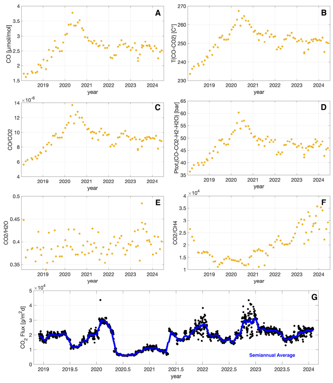
The SP hydrothermal system exhibits complex geochemical dynamics. The time series analysis of various geochemical parameters provided valuable insights into the system’s temporal variations and underlying processes. Several key ratios were monitored, including T(CO–CO2) [°C], which represents the equilibrium temperature for the hydrothermal system, CO [μmol/mol], CO/CO2, CO2/H2O, CO2/CH4 ratio, and P(CO–CO2–H2–H2O) [bar], which indicate the equilibrium pressure. These parameters provided insight into gas composition shifts, which are indicative of changes within the magmatic system (Figure 2).
Panels 2A–D originate from the same fumarolic dataset acquired at Bocca Grande (Figure 1B), the main fumarolic vent of Solfatara, using an automatic station under a uniform sampling and analytical protocol. In this set, CO and the gas ratios (e.g., CO/CO2) are directly measured on the same samples, whereas T(CO–CO2) and P(CO–CO2–H2–H2O) are geothermobarometric indicators derived from those ratios through equilibrium relationships. Accordingly, a close co-variation among panels 2A–D is expected and reflects both their functional dependence and the common hydrothermal–magmatic forcing acting on the SP system; these panels should therefore not be interpreted as independent degrees of freedom.
CO measurements (Figure 2A): from 2018 to the beginning of May 2020, there was a notable increase in CO concentration. Post-May 2020, the concentration decreases rapidly until stabilizing around 2022. After 2022, the CO concentration exhibited fluctuations around a stable mean value. Post-2022 oscillations appear larger in amplitude and more regular in periodicity, whereas fluctuations between 2018 and 2021 were smaller in amplitude and less regular.
Equilibrium Temperature of the CO–CO2 System (Figure 2B): from 2018 to early to mid-May 2020, there was a significant increase in equilibrium temperature. Post-May 2020, the temperature decreased rapidly, stabilizing around 2022. After 2022, temperatures exhibited fluctuations around a stable mean. Post-2022 oscillations appear larger in amplitude and more regular in periodicity, whereas fluctuations between 2018 and 2021 were smaller in amplitude and less regular.
CO/CO2 Ratio (Figure 2C): from 2018 to May 2020, there was a significant increase in the CO/CO2 ratio. Post-2021, the ratio decreased rapidly, stabilizing around 2022. After 2022, the CO/CO2 ratio exhibited fluctuations around a stable mean, with oscillations appearing larger in amplitude and more regular in periodicity. Fluctuations between 2018 and 2021 were smaller in amplitude and less regular. The peak around June 2020 is a notable feature.
Equilibrium Pressure of the Hydrothermal System P(CO–CO2–H2–H2O) (Figure 2D): from 2018 to 2021, there was a notable increase in equilibrium pressure. Post-2021, the pressure decreased rapidly, stabilizing around 2022. After 2022, equilibrium pressure showed fluctuations around a stable mean, with oscillations appearing larger in amplitude and more regular in periodicity. Fluctuations between 2018 and 2021 were smaller in amplitude and less regular. The peak around 2021 is a notable feature.
CO2/H2O Ratio (Figure 2E): there is no significant increase in the CO2/H2O ratio during the entire time window. The CO2/H2O ratio exhibited fluctuations around a mean value that is slowly increasing, with oscillations appearing periodic and regular.
CO2/CH4 Ratio (Figure 2F): from 2018 to Decembre 2020, there was a decreasing in the CO2/CH4 ratio, with two main strong decrements (beginning of the 2018 and 2019). Post-2021, the ratio increased, exhibiting limited fluctuations around a stable mean until 2023, where oscillations are appearing periodic and regular, with high amplitude.

Appendix A.3. Variations in CO2 Fluxes at Pisciarelli and Their Implications

CO2 Flux measurements (Figure 2G): the Pisciarelli fumarolic site has been continuously monitored for CO2 emissions over a data interval spanning from 1 December 2018 to 30 May 2024. Figure 2G presents the time series analysed as a monthly moving average. The semi-annual average (blue curve) is presented here to highlight longer-term trends, as this continuous dataset exhibits high-frequency noise that makes smoothing necessary, unlike the other parameters which were sampled at lower resolution.
The time series reveals multiple peaks, most notably around early 2020, late 2021, and mid-late 2022, where the CO2 flux exceeded 3.5 × 10⁴ g/(m2·day). Significant reductions in CO2 emissions were observed, with the lowest flow values occurring around mid-2020 and mid-2022. Over the monitoring period, the detailed analysis of the CO2 flux at Pisciarelli highlights both short-term variability and long-term trends.
In summary, the SP hydrothermal system has exhibited significant variations across multiple geochemical parameters between 2018 and 2024. The period from 2018 to 2021 is generally characterized by increasing trends, reaching peaks around mid-2020 to 2021, followed by rapid declines and stabilization around 2022. Post-2022, the system shows fluctuations that tend to be larger in amplitude and more regular in periodicity, suggesting the establishment of a new equilibrium state potentially influenced by cyclic external factors.

Appendix A.4. Spatial and Temporal Evolution of Surface Thermal Anomalies

The thermal dataset extends beyond those presented in [26]. Figure 3 integrates spatial and temporal analyses, illustrating the heating dynamics through land surface temperature (LST) and statistical trends.
Specifically, Figure 3A shows mean and annual thermal maps from 2020 to 2024. In Figure 3B, the LST time-series plot illustrates measured temperatures (black), de-seasonalized temperatures (red), and seasonal trends (green) are reported. The data reveal a pronounced seasonal cycle (green) superimposed on broader temperature variations. De-seasonalized temperatures (modelled through a sinusoidal regression and subtracted the retrieved best-fit pattern from the original dataset as suggested by [27]) isolate long-term thermal anomalies, providing insights into subsurface processes. Figure 3C focuses on de-seasonalized temperatures (red) alongside their six-month moving average (black). The smoothed trendline offers a clearer visualization of gradual temperature changes, indicating potential long-term geothermal or hydrothermal dynamics in the study area. Figure 3D shows the heat flux time series (blue) and the heat release rates (red). The consistent hotspots in mean map (red/yellow zones in Figure 3A) suggest persistent thermal anomaly activity, providing a comprehensive view of the thermal behaviour over the analysed period. Specifically, the mean annual map highlights two dominant patterns of thermal activity within the studied area. The first pattern, located on the right side of the maps, corresponds to the Pisciarelli mud pool area, exhibiting the highest thermal anomalies, with intense red zones persisting across all years, likely due to concentrated hydrothermal venting and localized geothermal heat flux. The second notable anomaly pattern is observed along the external flank of the Solfatara volcano, specifically near Via Scarfoglio area on the left side of the maps. This region consistently displays medium-to-low thermal anomalies (green-to-yellow zones), indicative of diffuse heat flow and potential subsurface thermal activity extending from the Solfatara hydrothermal system. Summarizing the observations: (i) Pisciarelli anomaly is a persistent and intense hotspot with slight interannual variability in intensity and spatial extent, representing the core of hydrothermal venting and geothermal heat emission. (ii) Via Scarfoglio Pattern consists of a diffuse and moderate heat flow along the external flank of the Solfatara volcano, showing gradual spatial expansion over time, potentially linked to subsurface dynamics. (iii) The temporal evolution of the LST field emphasizes that year 2022 is remarkable for an increased thermal activity, particularly in the Pisciarelli zone (Figure 3C) even if the overall spatial distribution of thermal anomalies remains consistent. Accordingly, a computed heat flow time series derived from the UAV-based thermal dataset from September 2019 to October 2023 is reported in Figure 3D, with a variable temporal resolution in function of the collected thermal images (minimum value 1 month). Specifically, the heat flux is computed according to [26,37], where k-means and DBSCAN algorithms are applied to thermal images to separate hot zones from the background temperature, and then to evaluate the heat flux for homogeneous zones using heat transfer model. Here, Figure 3D shows the estimated heat flux trend (in blue), and its variation (in red), having the lowest correlation with temperature one, which is nearby the Pisciarelli mud pool area.
Recurring peaks are observed approximately every 8–12 months, suggesting a quasi-seasonal to annual modulation of surface degassing and heat release. These maxima are mirrored by corresponding increases in the heat flux variations (red line), confirming that the system responds with coherent excursions in both absolute flux and its rate of change.
The highest fluxes occur around mid-2020 and mid-2022, with closely associated maxima in the variation curve. Other significant peaks are recorded in mid-2021 and mid-2023, though with comparatively lower amplitudes. Following each major maximum, the flux systematically decays to minima, as observed in late 2020, early 2021, and early 2022. A comparative analysis between heat flux and its variations (Figure 3D) reveals important correlations. The strong correspondence between the absolute heat flux (blue) and its variation (red) indicates that short-term increments in flux are systematically captured by the derivative metric. The period between mid-2022 and mid-2023 is characterized by elevated activity, with multiple successive peaks and shorter quiescence intervals compared to previous years. The most prominent peak in mid-2022, is glaring in both heat flux (blue) and its variations (red), suggesting a system-wide thermal perturbation.
Overall, the figure documents a strongly non-stationary thermal regime at Pisciarelli, marked by cyclic yet irregular heat flux surges and sharp variations. The persistence of high-amplitude oscillations and their apparent intensification in 2022–2023 may reflect evolving pressurization processes within the shallow hydrothermal system, which could have implications for hazard assessment and ongoing volcanic monitoring at Campi Flegrei.

Appendix A.5. Seismic Activity and Clustering Beneath the Hydrothermal Area

In the present study, the CF seismic catalogue was analysed using the DBSCAN algorithm to identify and characterize spatial clusters of seismic activity. This method, particularly suited for datasets with varying density distributions, enables the detection of regions where seismic events are densely concentrated while distinguishing isolated events considered noise. The clustering procedure used a search radius of 206 m and a minimum cluster size of six events, calibrated to the dimensionality of the spatial input matrix. These parameters were selected to robustly isolate meaningful seismic structures while minimizing spurious groupings. The results of this analysis provide a refined picture of the seismic dynamics within the caldera, offering critical insights into the spatial organization of earthquakes and their potential connection to underlying geological structures. The outcomes of the clustering analysis are illustrated in Figure 4, where the spatial distribution of seismic clusters is represented through contour lines depicting event density.
The plan view (Figure 4A) offers an overview of how seismicity is distributed across the Campi Flegrei area, with different clusters identified by distinct colours. The contour lines effectively highlight the areas with the highest concentration of earthquakes, delineating regions of intensified seismic activity. To further investigate the depth distribution of these clusters, two vertical cross-sections were considered. The North-South cross-section (Figure 4B) provides a view of how seismicity extends in depth along this axis, revealing well-defined zones of high activity. Similarly, the East-West cross-section (Figure 4C) confirms the presence of deep-seated clusters and highlights their spatial correlation with shallow seismicity, suggesting a structured arrangement of events that may be influenced by fault networks and magmatic or hydrothermal processes. Among the various clusters identified, particular attention is given to Cluster 1, located directly beneath the SP area. The seismicity associated with this cluster presents a highly concentrated pattern, both laterally and in depth, and is likely influenced by subsurface fluid movements and stress accumulation within the volcanic system. Given its strategic location and relevance, this study will focus specifically on the seismic events belonging to Cluster 1, aiming to investigate their temporal evolution and potential implications for the dynamic behaviour of the SP hydrothermal system. The spatial clustering results obtained through DBSCAN not only confirm the presence of localized zones of high seismicity but also provide essential clues regarding the interaction between tectonic and magmatic processes within Campi Flegrei. The density contours reveal that earthquake distribution is not random but follows specific structural trends, reinforcing the hypothesis that seismicity in the area is closely linked to the caldera’s ongoing geodynamic evolution. The identification and analysis of these clusters contribute to a deeper understanding of the mechanisms driving volcanic unrest, such as fluid migration and/or fault activities.
We analysed the earthquake catalogue by subdividing it into monthly intervals and computing the cumulative number of earthquakes for each month. On this basis, we estimated the probability density function (PDF) of seismic occurrence, which provides a continuous representation of the underlying distribution of events rather than relying solely on discrete counts. In our implementation we used the MATLAB (v2024a) Statistics and Machine Learning Toolbox function ksdensity to compute the kernel-smoothed density of earthquake occurrence times. This function allows specification of the kernel (we used Gaussian) and the bandwidth parameter, and returns the estimated density evaluated on a regular temporal grid. The resulting values (events per month) were used as the seismic occurrence rate density throughout the analysis (See Appendix B for further explanations). This estimation was specifically applied to the Cluster 1 subset of the INGV earthquake catalogue of Campi Flegrei, in order to characterize the temporal patterns of seismicity within that group.
From 2018 to the end of 2020, seismicity Occurrence Probability Density (OPD) remained relatively low and stable, indicating minimal seismic activity in the region. A gradual increase became evident starting in 2020, suggesting a progressive intensification of the underlying geological processes. This trend continues, culminating in a significant rise between 2022 and 2023, marking a period of pronounced seismic activity. In 2023, the seismicity OPD reached its peak, followed by fluctuations in early 2024. These variations may be attributed to changes in underground pressure, fluid migration, or small-scale eruptive dynamics. Toward the latest part of the dataset in 2024, a slight decline in seismicity density is observed, potentially indicating a temporary stabilization or a reduction in subsurface activity.
Overall, the data highlight a phase of increased seismic activity in SP, which may be linked to ongoing volcanic or geothermal processes. A more detailed analysis integrating geophysical and geochemical parameters would be necessary to further elucidate the mechanisms driving these observed seismic trends.

Appendix A.6. Ground Deformation as an Indicator of Subsurface Processes

The vertical ground deformation in the Pisciarelli area, derived from InSAR data and based on the average of four coherent SAR pixels within the region of interest, exhibits notable spatial and temporal characteristics. Spatially, the mean ground velocity map (Figure 5A) highlights a well-defined uplift area, with maximum velocities exceeding 12 cm/year.
The deformation pattern decreases radially from the central uplift, forming a gradient consistent with subsurface processes such as hydrothermal activity. The vertical component was then used to compute the monthly deformation rate, which was smoothed using a six-month moving average. Temporally, the cumulative deformation time series (Figure 5B) shows a continuous and steady increase from 2018 to 2024, reaching a total displacement of approximately 45 cm by the end of the observation period (for the pixels in Pisciarelli area). The near-linear trend in cumulative deformation indicates persistent driving forces in the system, likely related to pressurization or volumetric expansion within the subsurface structure. The time series of vertical deformation rates (Figure 5C) provides a more detailed view of the temporal variability. The rates exhibit oscillatory behaviour, with periods of acceleration and deceleration. Peaks in deformation rate occur around 2019, 2021, and late 2023, suggesting episodic intensifications in the processes driving deformation. The semi-annual moving average captures overall trends while smoothing short-term fluctuations, showing a general increase in deformation activity punctuated by temporary slowdowns. The dataset, collected with high temporal resolution (~12 days) and spatial resolution (~90 m), effectively captures both the localized nature and dynamic evolution of the deformation. The observed patterns suggest a strong connection between subsurface processes and surface deformation, emphasizing the importance of continuous InSAR monitoring for understanding the ongoing dynamics of the Pisciarelli area.

Appendix B

Appendix B.1. Seismic PDF and Kernel-Based Occurrence Rate Density (OPD)

To obtain a physically meaningful and continuous representation of the temporal evolution of seismicity, we computed the seismic Probability Density Function (PDF) of earthquake occurrence, used throughout the manuscript as a proxy for the dynamical state of the system. In our formulation, the seismic PDF represents the kernel-smoothed occurrence rate density of earthquakes, not a probability in the statistical sense.
The PDF is obtained through a Kernel Density Estimation (KDE) applied to the occurrence times of earthquakes in the local catalogue. For a set of event times ti, the KDE is defined as:
P D F t = O P D t = f ^ t = 1 n h i = 1 n K t t i h
where
n is the number of earthquakes,
h is the temporal bandwidth,
K(…) is a normalized kernel function (a Gaussian kernel was used).
The resulting quantity has unit events per month, consistent with the temporal resolution of the other datasets (uplift rate, CO2 flux, fumarole temperature) and represents the local density of seismic occurrence within the temporal window defined by the kernel.
Although the term Probability Density Function is used for continuity with previous literature on critical transitions and stability indicators, in this work the seismic PDF strictly corresponds to a non-probabilistic density function, i.e., a kernel-smoothed occurrence rate. For this reason, the quantity is not bounded between 0 and 1. Its magnitude reflects the instantaneous concentration of earthquakes per unit time rather than the probability of occurrence of a specific event. Values below 1 simply correspond to periods of low to moderate seismicity (2018–2022), while the increase in 2023–2024 reflects the well-documented rise in seismic activity during this interval. This smoothed representation avoids discontinuities associated with discrete monthly counting and reduces the influence of short-lived clusters, making the PDF a stable and robust indicator of the evolving state of the system. In this framework, the seismic PDF is used as a continuous proxy of the underlying stress to strain evolution and is analytically treated in the same manner as the PDFs derived for deformation and geochemical signals. Its continuous nature is essential for computing derivatives, normalized increments, and multivariate stability indicators used in the subsequent analyses.

Appendix B.2. Analytical Expression of the KDE

Given a series of event occurrence times t1, t2 …, tm, the Kernel Density Estimation (KDE) is defined as expressed in Equation (A1), where n is the number of events, h > 0 is the bandwidth, i.e., the smoothing window width, and K(…) is a normalized kernel function, satisfying:
+ K u d u = 1
For the commonly used Gaussian kernel, one has
K u = 1 2 π e u 2 2
and the KDE becomes
f ^ t = 1 n h 2 π i = 1 n e x p 1 2 t t i h 2
This function represents a continuous density of event occurrence (events per unit time), which in our study is expressed on a monthly time scale. In this context, the estimated function has physical units of 1/time (here: events per month) and represents a density of event occurrence over time. This quantity describes the local concentration of earthquakes within the kernel smoothing window.
For a given time interval [a, b]:
a b f ^ t d t
yields
  • The expected number of events occurring in the interval [a, b], when the KDE is computed in its standard form (normalization over the n observed events), as done in this study
  • Or, alternatively
  • The probability that an event falls within [a, b]
  • Only if the event times ti and the estimated function are previously normalized over the total temporal domain, so that the integral over the entire interval equals 1.
In our framework, the KDE is used as an occurrence rate density (OPD) rather than a probability. Therefore, the integral over [a b] corresponds to the expected number of earthquakes within that interval, consistent with the physical interpretation of the seismic time-series.

References

  1. Caliro, S.; Chiodini, G.; Avino, R.; Carandente, A.; Cuoco, E.; Di Vito, M.A.; Minopoli, C.; Rufino, F.; Santi, A.; Lages, J.; et al. Escalation of caldera unrest indicated by increasing emission of isotopically light sulfur. Nat. Geosci. 2025, 18, 167–174. [Google Scholar] [CrossRef] [Scilit]
  2. Steinmann, L.; Spiess, V.; Sacchi, M. The Campi Flegrei caldera (Italy): Formation and evolution in interplay with sea-level variations since the Campanian Ignimbrite eruption at 39 ka. J. Volcanol. Geotherm. Res. 2016, 327, 361–374. [Google Scholar] [CrossRef] [Scilit]
  3. Orsi, G. Volcanic and deformation history of the Campi Flegrei volcanic field. In Campi Flegrei: A Restless Caldera in a Densely Populated Area; Springer: Berlin/Heidelberg, Germany, 2022; pp. 1–28. [Google Scholar] [CrossRef] [Scilit]
  4. Smith, V.C.; Isaia, R.; Pearce, N.J.G. Tephrostratigraphy and glass compositions of post-15 kyr Campi Flegrei eruptions: Implications for eruption history and chronostratigraphic markers. Quat. Sci. Rev. 2011, 30, 3638–3660. [Google Scholar] [CrossRef] [Scilit]
  5. Barone, A.; Gola, G.; Caliro, S.; Chiodini, G.; Tizzani, P.; Castaldo, R. Long-term thermo-fluid dynamic modeling of Solfatara hydrothermal system, Campi Flegrei caldera. J. Volcanol. Geotherm. Res. 2025, 459, 108277. [Google Scholar] [CrossRef] [Scilit]
  6. Isaia, R.; Vitale, S.; Di Giuseppe, M.G.; Iannuzzi, E.; D’Assisi Tramparulo, F.; Troiano, A. Stratigraphy, structure, and volcano-tectonic evolution of Solfatara maar-diatreme (Campi Flegrei, Italy). Geol. Soc. Am. Bull. 2015, 127, 1485–1504. [Google Scholar] [CrossRef] [Scilit]
  7. Troiano, A.; Di Giuseppe, M.G.; Isaia, R. 3D structure of the Campi Flegrei caldera central sector from short-period magnetotelluric imaging. Sci. Rep. 2022, 12, 20802. [Google Scholar] [CrossRef] [Scilit]
  8. Siniscalchi, A.; Tripaldi, S.; Romano, G.; Chiodini, G.; Improta, L.; Petrillo, Z.; D’Auria, L.; Caliro, S.; Avino, R. Reservoir structure and hydraulic properties of the Campi Flegrei geothermal system inferred by audiomagnetotellurics. J. Geophys. Res. Solid Earth 2019, 124, 5336–5356. [Google Scholar] [CrossRef] [Scilit]
  9. Giacomuzzi, G.; Chiarabba, C.; Bianco, F.; De Gori, P.; Piana Agostinetti, N. Tracking transient changes in the plumbing system at Campi Flegrei caldera. Earth Planet. Sci. Lett. 2024, 637, 118744. [Google Scholar] [CrossRef] [Scilit]
  10. Troiano, A.; Isaia, R.; Di Giuseppe, M.G.; Tramparulo, F.D.A.; Vitale, S. Deep electrical resistivity tomography for a 3D picture of the most active sector of Campi Flegrei caldera. Sci. Rep. 2019, 9, 15124. [Google Scholar] [CrossRef] [Scilit] [PubMed]
  11. Chiodini, G.; Todesco, M.; Caliro, S.; Del Gaudio, C.; Macedonio, G.; Russo, M. Magma degassing as a trigger of bradyseismic events: The case of Phlegrean Fields. Geophys. Res. Lett. 2003, 30, 1434. [Google Scholar] [CrossRef] [Scilit]
  12. Chiodini, G.; Caliro, S.; De Martino, P.; Avino, R.; Gherardi, F. Early signals of new volcanic unrest at Campi Flegrei caldera? Geology 2012, 40, 943–946. [Google Scholar] [CrossRef] [Scilit]
  13. Chiodini, G.; Vandemeulebrouck, J.; Caliro, S.; D’Auria, L.; De Martino, P.; Mangiacapra, A.; Petrillo, Z. Evidence of thermal-driven processes triggering the 2005–2014 unrest at Campi Flegrei caldera. Earth Planet. Sci. Lett. 2015, 414, 58–67. [Google Scholar] [CrossRef] [Scilit]
  14. Chiodini, G.; Caliro, S.; Avino, R.; Bagnato, E.; Capecchiacci, F.; Carandente, A.; Cardellini, C.; Minopoli, C.; Tamburello, G.; Tripaldi, S.; et al. The hydrothermal system of the Campi Flegrei caldera. In Campi Flegrei: A Restless Caldera in a Densely Populated Area; Orsi, G., D’Antonio, M., Civetta, L., Eds.; Springer: Berlin/Heidelberg, Germany, 2022; pp. 239–255. [Google Scholar] [CrossRef] [Scilit]
  15. Caliro, S.; Avino, R.; Capecchiacci, F.; Carandente, A.; Chiodini, G.; Cuoco, E.; Minopoli, C.; Rufino, F.; Santi, A.; Rizzo, A.L.; et al. Chemical and isotopic characterization of groundwater and thermal waters from the Campi Flegrei caldera (southern Italy). J. Volcanol. Geotherm. Res. 2025, 460, 108280. [Google Scholar] [CrossRef] [Scilit]
  16. Chiodini, G.; Avino, R.; Caliro, S.; Minopoli, C. Temperature and pressure gas geoindicators at the Solfatara fumaroles. Ann. Geophys. 2011, 54, 2. [Google Scholar] [CrossRef] [Scilit]
  17. Bevilacqua, A.; Neri, A.; De Martino, P.; Giudicepietro, F.; Macedonio, G.; Ricciolino, P. Accelerating upper crustal deformation and seismicity of Campi Flegrei caldera (Italy), during the 2000–2023 unrest. Commun. Earth Environ. 2024, 5, 742. [Google Scholar] [CrossRef] [Scilit]
  18. Giudicepietro, F.; Avino, R.; Bellucci Sessa, E.; Bevilacqua, A.; Bonano, M.; Caliro, S.; Casu, F.; De Cesare, W.; De Luca, C.; De Martino, P.; et al. Burst-like swarms in the Campi Flegrei caldera accelerating unrest from 2021 to 2024. Nat. Commun. 2025, 16, 1548. [Google Scholar] [CrossRef] [Scilit]
  19. D’Auria, L.; Pepe, S.; Castaldo, R.; Giudicepietro, F.; Macedonio, G.; Ricciolino, P.; Tizzani, P.; Casu, F.; Lanari, R.; Manzo, M.; et al. Magma injection beneath the urban area of Naples: A new mechanism for the 2012–2013 volcanic unrest at Campi Flegrei caldera. Sci. Rep. 2015, 5, 13100. [Google Scholar] [CrossRef] [Scilit]
  20. Pepe, S.; De Siena, L.; Barone, A.; Castaldo, R.; D’Auria, L.; Manzo, M.; Casu, F.; Fedi, M.; Lanari, R.; Bianco, F.; et al. Volcanic structures investigation through SAR and seismic interferometry. Remote Sens. Environ. 2019, 234, 111440. [Google Scholar] [CrossRef] [Scilit]
  21. Castaldo, R.; Tizzani, P.; Solaro, G. Inflating source imaging and stress/strain field analysis at Campi Flegrei caldera. Remote Sens. 2021, 13, 2298. [Google Scholar] [CrossRef] [Scilit]
  22. Tizzani, P.; Fernández, J.; Vitale, A.; Escayo, J.; Barone, A.; Castaldo, R.; Pepe, S.; De Novellis, V.; Solaro, G.; Pepe, A.; et al. 4D imaging of the volcano feeding system beneath Campi Flegrei caldera. Remote Sens. Environ. 2024, 315, 114480. [Google Scholar] [CrossRef] [Scilit]
  23. Barone, A.; Tizzani, P.; Pepe, A.; Fedi, M.; Castaldo, R. Improving finite element optimization of InSAR-derived deformation source using integrated multiscale approach. Remote Sens. 2025, 17, 3237. [Google Scholar] [CrossRef] [Scilit]
  24. Tramelli, A.; Convertito, V.; Godano, C. B value enlightens different rheological behaviour in Campi Flegrei caldera. Commun. Earth Environ. 2024, 5, 275. [Google Scholar] [CrossRef] [Scilit]
  25. Scotto di Uccio, F.; Lomax, A.; Natale, J.; Muzellec, T.; Festa, G.; Nazeri, S.; Convertito, V.; Bobbio, A.; Strumia, C.; Zollo, A. Delineation and fine-scale structure of fault zones activated during the 2014–2024 unrest at the Campi Flegrei caldera (Southern Italy) from high-precision earthquake locations. Geophys. Res. Lett. 2024, 51, e2023GL107680. [Google Scholar] [CrossRef] [Scilit]
  26. Marotta, E.; Peluso, R.; Avino, R.; Avvisati, G.; Bellucci Sessa, E.; Belviso, P.; Caputo, T.; Carandente, A.; Cirillo, F.; Pescione, R.A. Clusterisation and temporal trends of heat flux by UAS thermal camera. Remote Sens. 2024, 16, 1102. [Google Scholar] [CrossRef] [Scilit]
  27. Mercogliano, F.; Barone, A.; D’Auria, L.; Castaldo, R.; Silvestri, M.; Bellucci Sessa, E.; Caputo, T.; Stroppiana, D.; Caliro, S.; Minopoli, C.; et al. Thermal patterns at the Campi Flegrei caldera inferred from satellite data and independent component analysis. Remote Sens. 2024, 16, 4615. [Google Scholar] [CrossRef] [Scilit]
  28. Royston, P.; Sauerbrei, W. Multivariable Model-Building: A Pragmatic Approach to Regression Anaylsis Based on Fractional Polynomials for Modelling Continuous Variables; John Wiley & Sons: Hoboken, NJ, USA, 2008. [Google Scholar]
  29. Rabinowitz, P.H. Minimax Methods in Critical Point Theory with Applications to Differential Equations; CBMS Regional Conference Series in Mathematics; American Mathematical Society: Providence, RI, USA, 1986; Volume 65. [Google Scholar]
  30. Cardellini, C.; Chiodini, G.; Frondini, F.; Avino, R.; Bagnato, E.; Caliro, S.; Lelli, M.; Rosiello, A. Monitoring diffuse volcanic degassing during volcanic unrests: The case of Campi Flegrei (Italy). Sci. Rep. 2017, 7, 6757. [Google Scholar] [CrossRef] [Scilit]
  31. Petrillo, Z.; Chiodini, G.; Mangiacapra, A.; Caliro, S.; Capuano, P.; Russo, G.; Cardellini, C.; Avino, R. Defining a 3D physical model for hydrothermal circulation. J. Volcanol. Geotherm. Res. 2013, 264, 172–183. [Google Scholar] [CrossRef] [Scilit]
  32. Ester, M.; Kriegel, H.-P.; Sander, J.; Xu, X. A density-based algorithm for discovering clusters in large spatial databases with noise. In KDD; AAAI Press: Washington, DC, USA, 1996; pp. 226–231. [Google Scholar]
  33. Cirillo, F.; Avvisati, G.; Belviso, P.; Marotta, E.; Peluso, R.; Pescione, R. STARTED: Statistical Analysis of Clustered Thermal Data; Zenodo: Geneva, Switzerland, 2022. [Google Scholar] [CrossRef]
  34. Giggenbach, W.F. A simple method for the collection and analysis of volcanic gas samples. Bull. Volcanol. 1975, 39, 132–145. [Google Scholar] [CrossRef] [Scilit]
  35. Giggenbach, W.F.; Gouguel, R.L. Collection and Analysis of Geothermal and Volcanic Water and Gas Discharges; DSIR Report CD2401; Department of Scientific and Industrial Research (DSIR), Chemistry Division: New Delhi, India, 1989. [Google Scholar]
  36. Cioni, R.; Corazza, E. Medium-temperature fumarolic gas sampling. Bull. Volcanol. 1981, 44, 23–29. [Google Scholar] [CrossRef] [Scilit]
  37. Marotta, E.; Peluso, R.; Avino, R.; Belviso, P.; Caliro, S.; Carandente, A.; Chiodini, G.; Macedonio, G.; Avvisati, G.; Marfè, B. Thermal energy release measurement with thermal camera: The case of La Solfatara volcano (Italy). Remote Sens. 2019, 11, 167. [Google Scholar] [CrossRef] [Scilit]
  38. Peluso, R. SERENADE—Seismic Database; Zenodo: Geneva, Switzerland, 2018. [Google Scholar] [CrossRef]
  39. Peluso, R. SERENADE Database Description; Miscellanea INGV; Istituto Nazionale di Geofisica e Vulcanologia (INGV): Rome, Italy, 2020; Volume 57, p. 7. [Google Scholar] [CrossRef]
  40. Ricciolino, P.; Lo Bascio, D.; Esposito, R. GOSSIP: Seismic Database; INGV: Rome, Italy, 2024. [Google Scholar] [CrossRef]
  41. Lee, W.H.K.; Lahr, J.C. HYPO71: A Computer Program for Determining Hypocenters. USGS Open-File Report 75-311; U.S. Geological Survey (USGS): Reston, VA, USA, 1975.
  42. Johnson, C.E.; Bittenbinder, A.; Bogaert, B.; Dietz, L.; Kohler, W. Earthworm: A flexible approach to seismic network processing. IRIS Newsl. 1995, 14, 1–4. [Google Scholar]
  43. Di Filippo, A.; Peluso, R. SEREWrap; Zenodo: Geneva, Switzerland, 2019. [Google Scholar] [CrossRef]
  44. Peluso, R. WESSEL; Zenodo: Geneva, Switzerland, 2018. [Google Scholar] [CrossRef]
  45. Berardino, P.; Fornaro, G.; Lanari, R.; Sansosti, E. A new algorithm for surface deformation monitoring based on small baseline differential SAR interferograms. IEEE Trans. Geosci. Remote Sens. 2002, 40, 2375–2383. [Google Scholar] [CrossRef] [Scilit]
  46. Jolivet, R.; Grandin, R.; Lasserre, C.; Doin, M.-P.; Peltzer, G. Systematic InSAR tropospheric phase delay corrections from global meteorological reanalysis data. Geophys. Res. Lett. 2011, 38, L17311. [Google Scholar] [CrossRef] [Scilit]
  47. Rosen, P.A.; Hensley, S.; Joughin, I.R.; Li, F.K.; Madsen, S.N.; Rodriguez, E.; Goldstein, R.M. Synthetic aperture radar interferometry. Proc. IEEE 2000, 88, 333–382. [Google Scholar] [CrossRef] [Scilit]
  48. Manzo, M.; Ricciardi, G.P.; Casu, F.; Ventura, G.; Zeni, G.; Borgström, S.; Berardino, P.; Del Gaudio, C.; Lanari, R. Surface deformation at Ischia Island. J. Volcanol. Geotherm. Res. 2006, 151, 399–416. [Google Scholar] [CrossRef] [Scilit]
  49. Pepe, A.; Solaro, G.; Calò, F.; Dema, C. A minimum acceleration approach for InSAR time series. IEEE J. Sel. Top. Appl. Earth Obs. Remote Sens. 2016, 9, 3883–3898. [Google Scholar] [CrossRef] [Scilit]
  50. Finkel, S.S. Linear panel analysis. In Handbook of Longitudinal Research; Elsevier: Amsterdam, The Netherlands, 2007. [Google Scholar]
  51. Shorrocks, A.F. Decomposition procedures for distributional analysis. J. Econ. Inequal. 2013, 11, 99–126. [Google Scholar] [CrossRef] [Scilit]
  52. Kutner, M.H.; Nachtsheim, C.J.; Neter, J.; Li, W. Applied Linear Statistical Models, 5th ed.; McGraw-Hill/Irwin: New York, NY, USA, 2005. [Google Scholar]
  53. Suleiman, A.A. Analysis of multicollinearity in multiple regressions. Int. J. Adv. Technol. Eng. Sci. 2015, 3, 571–578. [Google Scholar]
  54. Fletcher, R. Practical Methods of Optimization; John Wiley & Sons: Hoboken, NJ, USA, 2013. [Google Scholar]
  55. Karmarkar, N. A new polynomial-time algorithm for linear programming. Combinatorica 1984, 4, 373–395. [Google Scholar] [CrossRef] [Scilit]
  56. R Core Team. R: A Language and Environment for Statistical Computing; R Foundation: Vienna, Austria, 2014. [Google Scholar]
  57. Theußl, S.; Schwendinger, F.; Hornik, K. ROI: An extensible R optimization infrastructure. J. Stat. Softw. 2020, 94, 1–64. [Google Scholar] [CrossRef] [Scilit]
  58. Boyd, S.; Vandenberghe, L. Convex Optimization; Cambridge University Press: Cambridge, UK, 2004. [Google Scholar]
  59. Wickham, H. ggplot2: Elegant Graphics for Data Analysis; Springer: Berlin/Heidelberg, Germany, 2009. [Google Scholar]
  60. Del Gaudio, C.; Aquino, I.; Ricciardi, G.P.; Ricco, C.; Scandone, R. Unrest episodes at Campi Flegrei: A reconstruction of vertical ground movements during 1905–2009. J. Volcanol. Geotherm. Res. 2010, 195, 48–56. [Google Scholar] [CrossRef] [Scilit]
  61. Vanorio, A.; Geremia, D.; De Landro, G.; Guo, T. Recurrence of geophysical manifestations at Campi Flegrei. Sci. Adv. 2025, 11, eadt2067. [Google Scholar] [CrossRef] [Scilit]
  62. Borgia, A.; Tizzani, P.; Solaro, G.; Manzo, M.; Casu, F.; Luongo, G.; Pepe, A.; Berardino, P.; Fornaro, G.; Sansosti, E.; et al. Volcanic spreading of Vesuvius. Geophys. Res. Lett. 2005, 32, L03303. [Google Scholar] [CrossRef] [Scilit]
  63. Newhall, C.G.; Pallister, J.S. Introducing the Volcanic Unrest Index. Bull. Volcanol. 2015, 77, 77. [Google Scholar] [CrossRef] [Scilit]
  64. Biggs, J.; Pritchard, M.E. Global satellite observations of magmatic and volcanic deformation. In Global Volcanic Hazards and Risk; Cambridge University Press: Cambridge, UK, 2016. [Google Scholar]
  65. Behr, Y.; Christophersen, A.; Miller, C. Probabilistic multi-sensor eruption forecasting. Geophys. Res. Lett. 2024, 51, e2024GL112029. [Google Scholar] [CrossRef] [Scilit]
  66. Scheffer, M.; Bascompte, J.; Brock, W.A.; Brovkin, V.; Carpenter, S.R.; Dakos, V.; Held, H.; van Nes, E.H.; Rietkerk, M.; Sugihara, G. Early-warning signals for critical transitions. Nature 2009, 461, 53–59. [Google Scholar] [CrossRef] [Scilit] [PubMed]
  67. Dakos, V.; Carpenter, S.R.; Brock, W.A.; Ellison, A.M.; Guttal, V.; Ives, A.R.; Kéfi, S.; Livina, V.; Seekell, D.A.; van Nes, E.H.; et al. Methods for Detecting Early Warnings of Critical Transitions in Time Series Illustrated Using Simulated Ecological Data. PLoS ONE 2012, 7, e41010. [Google Scholar] [CrossRef] [Scilit]
  68. Lenton, T.M. Environmental tipping points. Annu. Rev. Environ. Resour. 2013, 38, 1–29. [Google Scholar] [CrossRef] [Scilit]
  69. Boers, N. Observation-based early-warning signals for AMOC collapse. Nat. Clim. Change 2021, 11, 680–688. [Google Scholar] [CrossRef] [Scilit]
  70. Gualandi, A.; Liu, Z. Variational Bayesian independent component analysis for InSAR. J. Geophys. Res. Solid Earth 2021, 126, e2020JB020845. [Google Scholar] [CrossRef] [Scilit]
  71. Bernuzzi, S.; Boers, N. Critical slowing down in dynamical systems driven by nonstationary correlated noise. Phys. Rev. Res. 2022, 4, 013230. [Google Scholar] [CrossRef] [Scilit]
  72. GVMID Working Group. The Global Volcano Monitoring Infrastructure Database. Front. Earth Sci. 2024, 12, 1284889. [Google Scholar] [CrossRef] [Scilit]
  73. Potter, S.H.; Jolly, G.E.; Neall, V.E.; Johnston, D.M.; Scott, B.J. Communicating the status of volcanic activity: Revising New Zealand’s volcanic alert level system. J. Appl. Volcanol. 2014, 3, 13. [Google Scholar] [CrossRef] [Scilit]
  74. Bevilacqua, A.; Neri, A.; De Martino, P.; Isaia, R.; Novellino, A.; D’Assisi Tramparulo, F.; Vitale, S. Radial interpolation of GPS and leveling data of ground deformation in a resurgent caldera: Application to Campi Flegrei (Italy). J. Geod. 2020, 94, 13. [Google Scholar] [CrossRef] [Scilit]
Figure 1. Solfatara–Pisciarelli volcanic area and geochemical monitoring network. (A) An aerial view of the Campi Flegrei caldera and the main structural features of the study area; the red box indicates the enlarged study area in (B). (B) Outline of the study area: Solfatara crater on the left and the Pisciarelli fumarolic field on the right.
Remotesensing 18 01240 g001
Figure 2. Temporal evolution of key geochemical parameters and CO2 flux in the Solfatara–Pisciarelli system from 2018 to 2024. (A) CO concentration time series. (B) Equilibrium temperature (T(CO–CO2)) time series. (C) CO/CO2 ratio. (D) Equilibrium pressure (P(CO–CO2–H2–H2O)) time series indicating pressurization within the hydrothermal system. (E) CO2/H2O ratio reflecting variations in gas-water interaction and subsurface conditions. (F) CO2/CH4 ratio. (G) CO2 flux time series (black) and its semi-annual moving average (blue).
Remotesensing 18 01240 g002
Figure 3. Thermal anomalies and heat flow dynamics within the Pisciarelli area from UAV-based thermal mapping and time series analysis (2019–2024). (A) Mean and annual thermal map from 2020 to 2024. (B) LST time series plot illustrating measured temperatures (black), de-seasonalized temperatures (red), and seasonal trends (green). (C) De-seasonalized temperature time series (red) and related six-month moving average (black). (D) Heat flux time series (blue) and heat release rates (red).
Remotesensing 18 01240 g003
Figure 4. Seismic clustering and temporal evolution of seismic activity within the CFc (2018–2024). (A) Spatial distribution of seismic clusters within the CFc, mapped over the local topography. The different colours represent distinct clusters of seismic events. (B) North-South vertical cross-section showing the depth distribution of seismic clusters. (C) East-West cross-section of the seismic clusters. (D) Time series of the seismic Occurrence Probability Density (OPD).
Remotesensing 18 01240 g004
Figure 5. Vertical ground deformation in the Solfatara–Pisciarelli area based on InSAR measurements (2018–2024). (A) InSAR mean vertical velocity map showing deformation rates across the CFc. The map highlights considered SAR pixels centred near the Pisciarelli spring, with deformation rates exceeding 12 cm/year (red zones) and a radial decrease in deformation intensity toward the outer regions. (B) Cumulative vertical deformation time series derived from the average of coherent pixels within the Pisciarelli area, that are shown with different coloured asterisks. (C) Time series of vertical deformation rate (black) and the semi-annual moving average (blue).
Remotesensing 18 01240 g005
Figure 6. LAG and NO-LAG models comparative residuals analysis. In (A) LAG Model and in (B) NO-LAG Model. The blue dots indicate deformation data, red points model fitting and green ones the residuals.
Remotesensing 18 01240 g006
Figure 7. Covariate-adjusted deformation models illustrating the relationship between deformation and the others physical parameters. (A) Deformation as a function of its first lag. (B) Nonlinear positive correlation between seismic activity and deformation. (C) Negative correlation between equilibrium pressure P(CO–CO2–H2–H2O) and ground deformation. The shaded areas represent confidence intervals for the regression fits.
Remotesensing 18 01240 g007
Figure 8. Covariate-adjusted deformation models illustrating the influence of the considered physical and geochemical parameters on ground deformation. (A) Nonlinear positive relationship between seismic activity and deformation. (B) Negative correlation between temperature and deformation. (C) Positive correlation between heat flow and deformation. (D) Positive relationship between CO2 flow and deformation. (E) Negative correlation between equilibrium pressure P(CO–CO2–H2–H2O) and ground deformation. The shaded areas represent confidence intervals for the regression models.
Remotesensing 18 01240 g008
Figure 9. Individual time series for seismic activity, deformation, temperature, heat flow, CO2 flux, and P(CO–CO2–H2–H2O) and critical transitions. (A) 2018–2022 Interval and its critical transition on the 30 November 2020, highlighted by the dashed line. (B) 2018–2024 Interval and its critical transition on the 1 April 2023, highlighted by the dashed line.
Remotesensing 18 01240 g009
Figure 10. Bootstrap-derived distribution of Critical Points (CPs) and partitioned contributions of the covariates for the Solfatara–Pisciarelli system. (A) Bootstrap Distribution of the critical transition on the 30th of November 2020. (B) Shapley values showing the partitioned contribution of the covariates to identify the CP1. (C) Bootstrap Distribution of the critical transition on the 1st of April 2023. (D) Shapley values showing the partitioned contribution of the covariates to identify the CP2. Dashed lines in (A,B) are showing the CI limits.
Remotesensing 18 01240 g010
Table 1. Lag order selection criteria.
LagLLLRdfpFPEAICHQICSBIC
0−66.56---2.8240.66540.66540.6654
113.08159.28 *100.045108 *−3.47351 *−3.45818 *−3.43041 *
213.681.2210.270.046−3.4529−3.4222−3.3667
313.690.01410.9050.049−3.4006−3.3546−3.2713
414.341.28810.2560.050−3.3819−3.3205−3.2095
LL = Log Likelihood; LR = Likelihood Ratio; df = Degree of Freedom; p = probability (alfa error); FPE = Akaike’s Final Prediction Error criterion; AIC = Akaike Information criterion; HQIC = Hannan–Quinn information criterion; SBIC = Schwarz Bayesian information criterion. An ‘*’ indicates the optimal lag.
Table 2. Comparison between the lagged model (Panel A), used as the primary inferential specification because it accounts for temporal dependence in deformation, and the corresponding unlagged model (Panel B), reported for comparative purposes only. Predictor relevance should be interpreted jointly from partial R2 and bootstrap inclusion frequency.
Panel APanel B
Global R20.9990.97
AIC−24.0165.3
ParameterFun. FormCoeff.pR2p (%)BIF (%)Fun. FormCoeff.pR2p (%)BIF (%)
First LagLin.0.94≤0.00144.4100-----
Seismicity1/√x−0.49≤0.00134.297.71/√x−5.7≤0.00150.6100
TemperatureLin.0.008=0.36-16.4Lin.−0.22=0.0013.985.7
Heat FlowLin.−0.0001=0.43-21Lin.0.006≤0.0018.999.9
CO2 FlowLin.−0.00004=0.54-47.6Lin.0.0002≤0.0017.699.6
P(CO–CO2–H2–H2O)Lin.−0.04=0.00521.477.1Lin.−0.64≤0.0012997.7
CO2/H2OLin.−3.4=0.23-49.5Lin.−27.2=0.26-23.8
Constant-21.5≤0.001---24.4≤0.001--
Bold face marks the significant factors of each final model. AIC = Akaike Information Criterion. R2p = Fraction of explained variance. Fun. Form = Functional form. Coeff. = Coefficient. Lin. = Linear. p = observed alfa error. BIF = Bootstrap Inclusion Frequency.
Disclaimer/Publisher’s Note: The statements, opinions and data contained in all publications are solely those of the individual author(s) and contributor(s) and not of MDPI and/or the editor(s). MDPI and/or the editor(s) disclaim responsibility for any injury to people or property resulting from any ideas, methods, instructions or products referred to in the content.