Article

MS-DARNet: A Lightweight Multi-Scale Selective Dilated Attention Residual Network for Remote Sensing Scene Classification

by
Jiawei Huang
1 and
Chengjun Xu
2,3,*
1
School of Computer Science and Technology, Ocean University of China, Qingdao 266003, China
2
School of Artificial Intelligence, Jiangxi Normal University, Nanchang 330022, China
3
School of Remote Sensing and Information Engineering, Wuhan University, Wuhan 430072, China
*
Author to whom correspondence should be addressed.
Remote Sens. 2026, 18(8), 1235; https://doi.org/10.3390/rs18081235
Submission received: 4 March 2026 / Revised: 8 April 2026 / Accepted: 17 April 2026 / Published: 19 April 2026

Highlights

What are the main findings?
  • We developed MS-DARNet, which combines a Multi-branch Dilated Feature Extraction (MDFE) module and a Context-Position Aware Attention (CPAA) module to handle scale variations and complex background noise.
  • The proposed network achieves superior classification accuracies (97.78% on AID, 94.53% on NWPU-RESISC45, and 94.55% on RSD-WHU46) with a remarkably low complexity of only 2.50 M parameters and 0.5940 GMACs.
What are the implications of the main findings?
  • This model effectively balances the trade-off between computational efficiency and classification accuracy in the classification of high-resolution remote sensing scenes.
  • Its highly efficient and lightweight architecture demonstrates significant potential for practical deployment on resource-constrained Earth observation equipment.

Abstract

High-resolution remote sensing image (HRRSI) scene classification faces challenges such as significant target scale variations, complex background interference, and the difficult spatial parsing of dense objects (such as tightly packed buildings in dense residential areas or scattered aircraft on aprons), while existing models struggle to balance computational efficiency and classification accuracy. To address these issues, this paper proposes a lightweight Multi-Scale Selective Dilated Attention Residual Network (MS-DARNet). The model utilizes a Multi-branch Dilated Feature Extraction (MDFE) module, employing parallel convolutional branches with varying dilation rates to dynamically expand the receptive field and collaboratively extract multi-scale features without increasing parameter counts. Furthermore, a Context-Position Aware Attention (CPAA) module is introduced, combining a large kernel decomposition strategy to suppress irrelevant background noise with direction-aware feature aggregation to retain precise spatial coordinates for dense objects. Extensive experiments on the AID, NWPU-RESISC45, and RSD-WHU46 datasets show that MS-DARNet achieves superior classification accuracies of 97.78%, 94.53%, and 94.55%, respectively. Concurrently, it maintains a significantly low complexity of just 2.50 M parameters and 0.5940 GMACs. These findings demonstrate that MS-DARNet effectively achieves an optimal balance between lightweight architecture and exceptional classification performance for complex remote sensing scenes.

1. Introduction

Remote sensing images (RSIs), as comprehensive carriers recording Earth’s surface features, constitute the foundation of modern Earth exploration and observation systems [1,2]. With the rapid development of aerospace technology [3] and sensor performance [4], an increasing volume of high-resolution remote sensing images (HRRSIs) can be acquired. These images possess abundant spectral features and fine spatial textures, providing detailed data support for the structural representation of the Earth’s surface. As a fundamental and crucial task in HRRSI analysis, remote sensing scene classification (RSSC) has been widely applied in fields such as natural disaster monitoring [5], urban planning [6], land use analysis, and ecological environment protection [7], demonstrating immense significance. Therefore, the effective utilization of HRRSIs represents an important research topic.
However, compared to general object classification in natural images, RSSC faces unique challenges brought about by imaging altitudes, diverse sensors, and the broad coverage and diversity of ground areas:
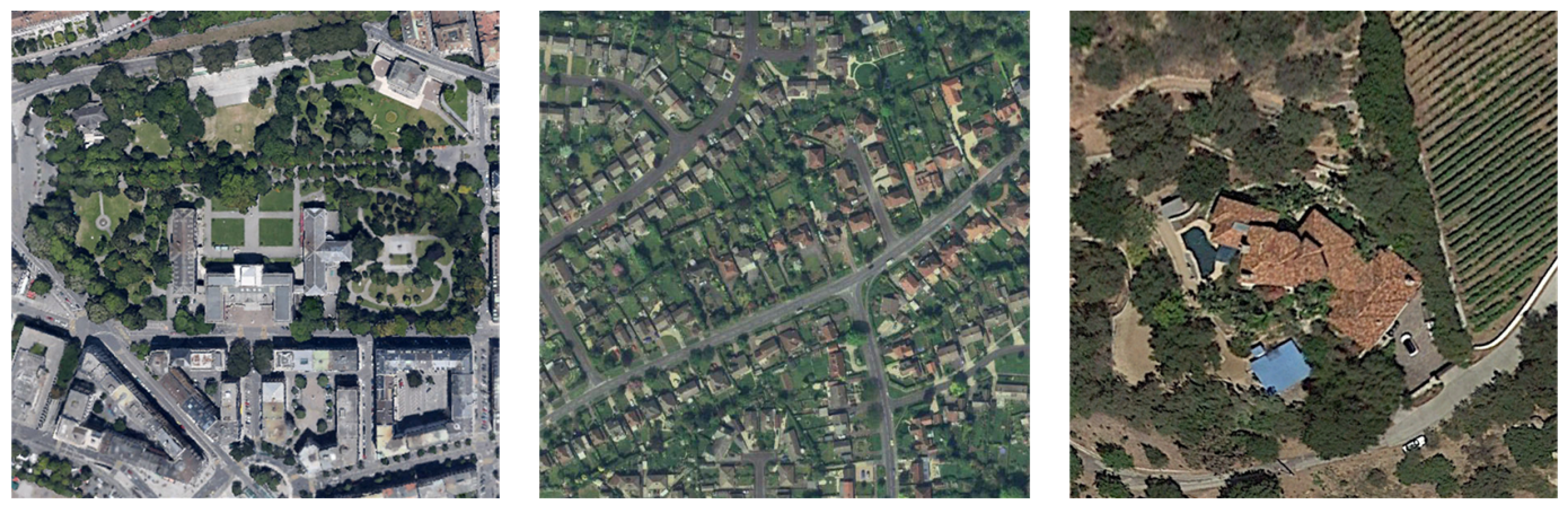
  • Significant scale variations in target objects: Objects of interest in remote sensing scenes exhibit massive differences in physical size. As shown in Figure 1, an “Airport” scene typically contains a runway spanning the entire image, necessitating a large receptive field to capture the global geometric structure. Concurrently, the “airplanes” on the apron in the same scene occupy only a few pixels, requiring fine-grained local feature extraction. However, traditional, fixed-size convolutional kernels struggle to simultaneously capture and learn features under both conditions [8].
2.
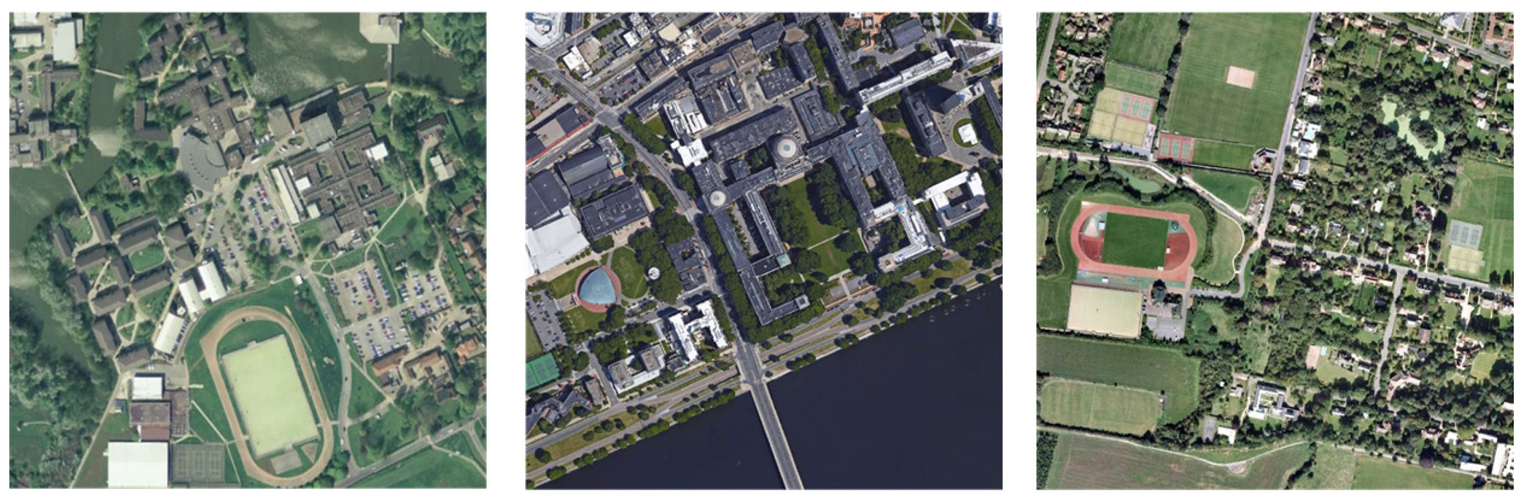
Strong interference from complex backgrounds: HRRSIs usually cover vast geographical areas, containing a substantial amount of background noise irrelevant to the semantic category. As illustrated in Figure 2, in a “school” scene, vegetation, playgrounds, and various buildings create strong visual interference that may confuse the model’s recognition. Unlike the human eye, which can naturally filter out such environmental disturbances, standard networks generally lack the selective capability to suppress this complex noise [10].
3.
Impact of spatial layout and structural distribution: Many scenes are characterized by densely arranged small objects, where spatial layout is key to classification [11]. As depicted in Figure 3, buildings and vegetation in “DenseResidential” and “School” scenes are tightly packed and highly repetitive. If a network relies solely on a global pooling mechanism that discards precise spatial coordinate information, it becomes exceedingly difficult to distinguish these scenes from others with similar structural distributions but different spatial layouts (such as “ SparseResidential”).
Traditional remote sensing scene classification research has primarily focused on designing effective manual feature extractors to capture the physical attributes and statistical regularities of images. Early low-level feature methods, such as Scale-Invariant Feature Transform (SIFT) [12] and Histogram of Oriented Gradients (HOG) [13], mainly described texture and shape information by detecting the gradient distribution of local keypoints. To further enhance the semantic representation capability of features, mid-level representation methods based on the Bag-of-Visual-Words (BoVW) model [14] were widely adopted; by constructing a visual dictionary through clustering algorithms, they neglected the spatial location of local features to a certain extent, thereby obtaining stronger translation invariance. However, these traditional methods inherently rely on shallow feature statistics, lacking the ability to model deep semantic structures and complex spatial contexts [15,16,17], making it difficult to cope with complex background interference and drastic scale variations in ground objects in HRRSIs.
With the widespread application of deep learning technology across various fields, Convolutional Neural Networks (CNNs) have rapidly become the mainstream owing to their powerful autonomous feature extraction capabilities, effectively overcoming the over-reliance of traditional handcrafted features on low-level physical attributes and significantly improving the model’s ability to abstract and generalize complex scene semantics [18,19,20]. For instance, RepFACNN, proposed by Shi et al. [21], achieved deep aggregation and efficient inference of multi-scale features within a pure convolutional framework via structural re-parameterization technology. LGNet, proposed by Xu et al. [22], adopted a dual-branch architecture combining Lie group spatial feature extraction with a multi-dimensional cross-attention mechanism, effectively balancing the model’s computational efficiency and feature representation capability. Additionally, SDLS, proposed by Ma et al. [23], constructed a two-stream architecture incorporating a self-distillation mechanism and a local feature stream; by simultaneously capturing local discriminative details and global semantic contexts, it effectively resolved feature confusion in complex scenes. Although deep learning has achieved higher classification accuracy compared to traditional handcrafted features, it still suffers from deficiencies in effectively building long-range dependency modeling, leading to difficulties in accurately identifying large-scale target objects and high model computational complexity.
To address the shortcomings in deep learning, researchers have introduced attention mechanisms into RSSC [24,25,26,27]. For example, SpectralGPT, constructed by Hong et al. [28], utilized the global perception capability of Transformers to process complex spatial-spectral correlations. Li et al. [29] proposed a lightweight remote sensing scene classification method based on ResNet-18 and attention mechanisms; by integrating Efficient Channel Attention (ECA) and self-attention modules, the network simultaneously enhanced focus on key image information and suppressed irrelevant background feature interference, effectively improving classification accuracy in complex scenes while significantly reducing the number of model parameters. Because the computational complexity of Transformers grows quadratically with resolution [30], limiting their application on resource-constrained devices, scholars subsequently proposed Mamba attention models based on linear complexity [31,32,33,34,35]. For instance, Li et al. [36] proposed Semi-Mamba, utilizing the linear complexity characteristics of State Space Models (SSMs) and selective scanning mechanisms to achieve efficient modeling of the global context of remote sensing images while effectively reducing memory consumption. G-VMamba, proposed by Yan et al. [37], designed a contour enhancement module and a dual-path feature extraction route, effectively enhancing the capture capability of ground object edge information while maintaining model lightweightness. Moreover, MPFASS-Net, constructed by Li et al. [38], combined the linear sequence modeling advantages of Mamba with a self-supervised learning strategy to achieve efficient aggregation and discriminative representation of multi-scale features in remote sensing images.
Although the aforementioned models have achieved certain results, the following deficiencies remain:
  • Limitations of fixed receptive fields: Most CNN architectures rely primarily on standard convolutional kernels with fixed sizes, lacking the ability to dynamically adapt to multi-scale features. This inherent physical limitation prevents the model from adaptively adjusting the receptive field range like a zoom lens, causing an inability to simultaneously balance the global semantic context of large-scale ground objects and the fine-grained texture features of minute targets at the same hierarchical level.
  • Limitations of traditional attention mechanisms: Most existing attention mechanisms lack fine-grained spatial selectivity and are prone to introducing irrelevant background noise interference. Furthermore, the Global Average Pooling (GAP) operation widely employed at the end of networks forcibly compresses spatial dimensions, resulting in the loss of crucial positional coordinate information, which restricts the model’s spatial structure parsing for densely arranged scenes [10].
  • Imbalance between computational performance and scene classification accuracy: To achieve high classification accuracy, existing models often suffer from complex structures, massive parameter counts, and heavy computational burdens. Conversely, lightweight models designed to alleviate computational burdens frequently sacrifice classification accuracy due to insufficient feature extraction capabilities, making it difficult to achieve ideal results in complex remote sensing scenes.
To solve the above problems, we propose the Multi-Scale Selective Dilated Attention Residual Network (MS-DARNet). Through the synergistic effect of Multi-branch Dilated Feature Extraction (MDFE) and the Context-Position Aware Attention (CPAA) mechanism, this model realizes dynamic perception of multi-scale remote sensing scenes and precise capture of background noise, effectively enhancing the model’s representation capability for complex remote sensing scene features while significantly reducing computational complexity. The contributions of this work are as follows:
  • To address the issue that fixed receptive fields struggle to adapt to target scale variations, we propose the MDFE module. Inspired by camera imaging principles, this module designs parallel “macro” and “wide-angle” branches. The “macro” branch utilizes a small dilation rate to capture local fine-grained textures, while the “wide-angle” branch uses a large dilation rate to cover large-scale global structures. By combining parallel dilated convolutions with cross-feature fusion, this module dynamically expands the effective receptive field without increasing parameter counts, effectively resolving the insufficiency of single-scale feature extraction.
  • To solve the problem that standard attention mechanisms are susceptible to background noise and lose spatial information, we design the Context-Position Aware Attention (CPAA) module. This module contains two core branches: first, it adopts a large-kernel decomposition strategy (5 × 5 + dilated 7 × 7) to simulate “selective attention,” effectively suppressing irrelevant background noise by aggregating long-range contexts; second, it introduces position-aware encoding, re-embedding coordinate information into features to restore spatial geometric attributes. This mechanism ensures the model remains highly sensitive to the spatial structure of dense objects, significantly boosting classification accuracy.
  • Aiming at the imbalance between computational performance and classification accuracy, we present the overall MS-DARNet architecture. We deploy a STEM layer at the front end of the model to rapidly reduce resolution while retaining rich information to alleviate computational burdens. Simultaneously, the model extensively employs dilated convolutions (such as branches with dilation rates of 2 and 4 in MDFE) to replace large-sized standard convolutions, dynamically expanding the receptive field while keeping the parameter count constant. This design effectively reduces model complexity while substantially enhancing its feature representation capability for HRRSIs.

2. Related Work

2.1. Remote Sensing Scene Classification Methods Based on Traditional Handcrafted Features

Traditional RSSC primarily relies on handcrafted feature extractors, and research in this stage typically encompasses methods based on low-level visual features and mid-level semantic representations. Early low-level methods focused on capturing the physical attributes of images. For instance, SIFT [12] describes local structures by detecting the gradient distribution of keypoints and their neighborhoods, possessing robust rotation and scale invariance; HOG [13] characterizes shape information by compiling histograms of oriented gradients in local image regions. Although these features perform well when processing simple scenes with uniform textures and fixed structures, they often struggle to extract discriminative semantic information when confronted with the complex backgrounds and diverse ground objects in HRRSIs, resulting in decreased scene classification accuracy. To overcome the limitations of traditional handcrafted feature methods, researchers introduced mid-level feature representations. A typical representative is BoVW [14], which constructs a visual dictionary through clustering algorithms and represents images as histograms of visual words, thereby neglecting the spatial locations of local features to attain stronger translation invariance. Subsequently, to mine the potential semantic co-occurrence relationships of visual words, probabilistic topic models such as Latent Dirichlet Allocation (LDA) [39] were introduced. However, these traditional methods essentially still rely on shallow feature statistics and lack the ability to learn deep scene structures and spatial contexts, which limits further improvements in classification accuracy.

2.2. Deep Learning-Based Remote Sensing Scene Classification Methods

The emergence of CNNs marked a new era of end-to-end feature learning for RSSC, fundamentally transforming the traditional paradigm that relied on manually designed low-level features. With the rapid advancement of deep learning technologies, modern architectures have shifted from early simple deep stacking to utilizing residual connections and multi-branch parallel structures to construct deeper and more efficient feature extractors. To overcome the limitations of traditional CNNs, recent research has focused on capturing global semantics precisely under a pure convolutional architecture by optimizing the geometric structure of convolutional kernels and designing pyramidal hierarchical feature fusion.
To address the severe target scale variations in remote sensing scenes, the latest research is dedicated to improving the context awareness of networks by altering the size of convolutional kernels. For example, Zhang et al. [40] proposed a Large Kernel Separable Mixed Convolutional Network (LSMNet), which introduces extremely large convolutional kernels (such as 21 × 21 ) and utilizes a spatial and channel mixed encoding strategy. This approach breaks through the physical receptive field limitations of traditional 3 × 3 convolutions while avoiding a surge in parameters, achieving precise capture of the global geometric structure of large-scale ground objects within a pure convolutional architecture. To further resolve the issue of deep networks easily losing shallow features during multi-scale fusion, LFNet, proposed by Li et al. [41], introduces a frequency-domain-texture fusion mechanism and a distance correlation loss. By capturing global dependencies in the frequency domain, it effectively compensates for the shortcomings of pure spatial convolutions regarding long-range feature interactions. Nevertheless, such large-kernel or frequency-domain transformation methods suffer from drawbacks including massive parameter counts and heavy computational burdens, making it difficult to deploy these models on resource-constrained devices.
To achieve high-precision interpretation of complex ground objects under limited computational resources, lightweight models and knowledge distillation techniques have become research hotspots. For instance, addressing the characteristic high background noise in remote sensing images, Shi et al. [42] proposed an Inverted Residual Cross Head Knowledge Distillation Network (IRCHKD). This method builds an efficient feature extraction backbone using inverted residual blocks and “compresses” the deep discriminative knowledge of the teacher network into the student network via a cross-head distillation mechanism, effectively reducing the parameter count (to only 1.35 M) while maintaining high-precision classification performance. Furthermore, to tackle the excessive computational overhead of traditional networks, Fazilov et al. [43] presented a multi-feature fusion framework based on DMCCA (Discriminative Multiple Canonical Correlation Analysis). By mapping the heterogeneous deep features extracted by ResNet and DenseNet into a unified discriminative latent space, it effectively enhances inter-class separability. Although this method successfully reduces parameters, its non-end-to-end two-stage training mode (separating feature extraction from fusion and classification) restricts the dynamic fine-tuning capability of the feature extractor for specific tasks, leading to reduced classification accuracy.

2.3. Remote Sensing Scene Classification Based on Attention Mechanisms and State Space Models

To resolve the deficiency of CNNs in long-range dependency modeling, researchers have introduced attention mechanisms. As an illustration, Duan et al. [44] proposed a multi-scale fusion network based on Swin Transformer (STMSF). This study utilizes the unique Shifted Window Self-Attention mechanism of the Swin Transformer to achieve global information interaction across windows while limiting computational costs. By constructing a multi-level feature pyramid, the model simultaneously captures the macroscopic geometric structures of airport runways and the microscopic texture details of airplanes on the apron. On the NWPU-RESISC45 dataset, this model achieved a 3.42% increase in classification accuracy compared to the CNN-based VGG16 network. Furthermore, to further mine the discriminability of features, Zhang et al. [45] proposed SDT2Net, constructing a second-order differentiable token Transformer network. By introducing a Differentiable Token Compression (DTC) module into the self-attention mechanism, it utilizes second-order statistical features to adaptively filter critical visual tokens, effectively reducing redundant computations while enhancing the semantic capture capability of complex scenes. However, the calculation of high-dimensional feature second-order statistics involved in this method significantly increases memory overhead during training, and the complex dynamic token filtering process somewhat restricts the real-time inference speed of the model on large-scale data.
Although attention mechanisms resolve the long-range dependency modeling issue of CNNs, the computational complexity of such methods (including the Transformer architecture) grows quadratically as resolution increases, compounding the computational burden and consuming substantial memory. To break this bottleneck, researchers have proposed a series of Mamba-based remote sensing scene classification models [32,33,34,35,36,46,47,48,49]. For instance, targeting visible light scene classification, Chen et al. [46] proposed RSMamba, designing a dynamic multi-path activation mechanism to solve the direction-sensitivity issue of visual state space modeling. It achieved a classification accuracy of 93.85% on the NWPU-RESISC45 dataset with a parameter count of merely 5.7 M. To further enhance computational efficiency, Dong et al. [16] proposed LMHMamba (Lightweight Multifeature Hybrid Mamba). This approach combines the implicit high-dimensional feature generation of StarNet with a lightweight state space module; through a hybrid multi-scale feature extraction strategy, it effectively reduces the parameter count (only 1.35 M) while achieving efficient aggregation of local and global features. Addressing the challenge of spatial-spectral collaborative modeling in hyperspectral images, S2Mamba, developed by Wang et al. [47], utilized a Spatial-Spectral Mixture Gate mechanism to achieve dynamic fusion of two-stream features, attaining an accuracy of 97.50% on the Indian Pines dataset. SpectralMamba, proposed by Zhao et al. [35], focuses on lightweight design; combining efficient gated convolutions with SSM, it achieved a 99.12% accuracy on the Indian Pines dataset utilizing only 0.84 M parameters. Moreover, the advantages of Mamba have been extended to other remote sensing tasks, such as ChangeMamba proposed by Chen et al. [31], which utilizes a spatiotemporal state space model to process bitemporal images, achieving an F1 score exceeding 90% on the LEVIR-CD change detection dataset, thereby proving the broad potential of this architecture in processing multi-modal and multi-temporal remote sensing data. While this method effectively reduces parameters, it sacrifices classification accuracy on extreme samples.
Overall, MS-DARNet should be positioned primarily as an accuracy-oriented and highly compact alternative within the CNN family. It achieves efficient multi-scale global perception without the heavy memory footprint and computational burden associated with Transformer and Mamba-style models, making it highly suitable for resource-limited devices.

3. Methods

3.1. Overview

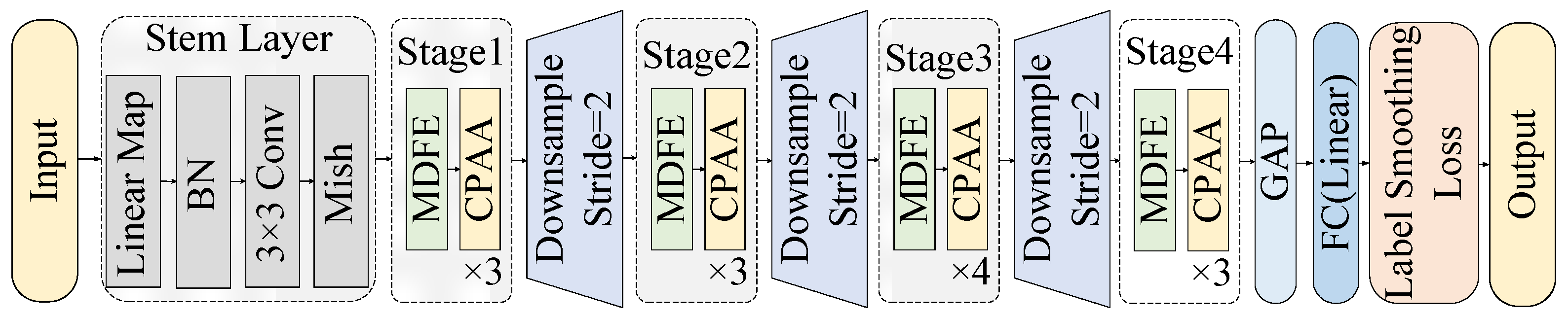
The architecture of the MS-DARNet model is illustrated in Figure 4. This architecture primarily consists of a STEM layer for initial feature mapping, four feature encoding stages (Stages), downsampling modules between stages, and a classification head. The STEM layer transforms the input image from the original pixel space into a preliminary feature representation. The four consecutive encoding stages are composed of MDFE modules and CPAA modules, which extract rich multi-scale semantic features from the feature maps and precisely capture crucial spatial location information. The downsampling modules are responsible for constructing a pyramid-shaped feature hierarchy, gradually expanding the receptive field to enhance global perception capabilities. Finally, the GAP and fully connected layers output the prediction results, and a label smoothing loss is calculated in conjunction with the ground truth labels during the training phase to optimize model parameters.

3.2. Stem Block

The structure of our Stem layer is shown in Figure 4, and its formulas are as follows
F m a p = L A X i n
F s t e m = M i s h C o n v 3 × 3 B N F m a p
where X i n R H × W × C denotes the input original remote sensing image, and H , W , and C represent the height, width, and number of channels of the image, respectively. L A represents the initial linear mapping operation, F m a p indicates the intermediate feature embedding after linear mapping, and B N stands for the Batch Normalization operation. C o n v 3 × 3 denotes a standard convolution with a kernel size of 3 × 3 , M i s h represents the Mish non-linear activation function, and F s t e m is the final feature map output by the Stem module.
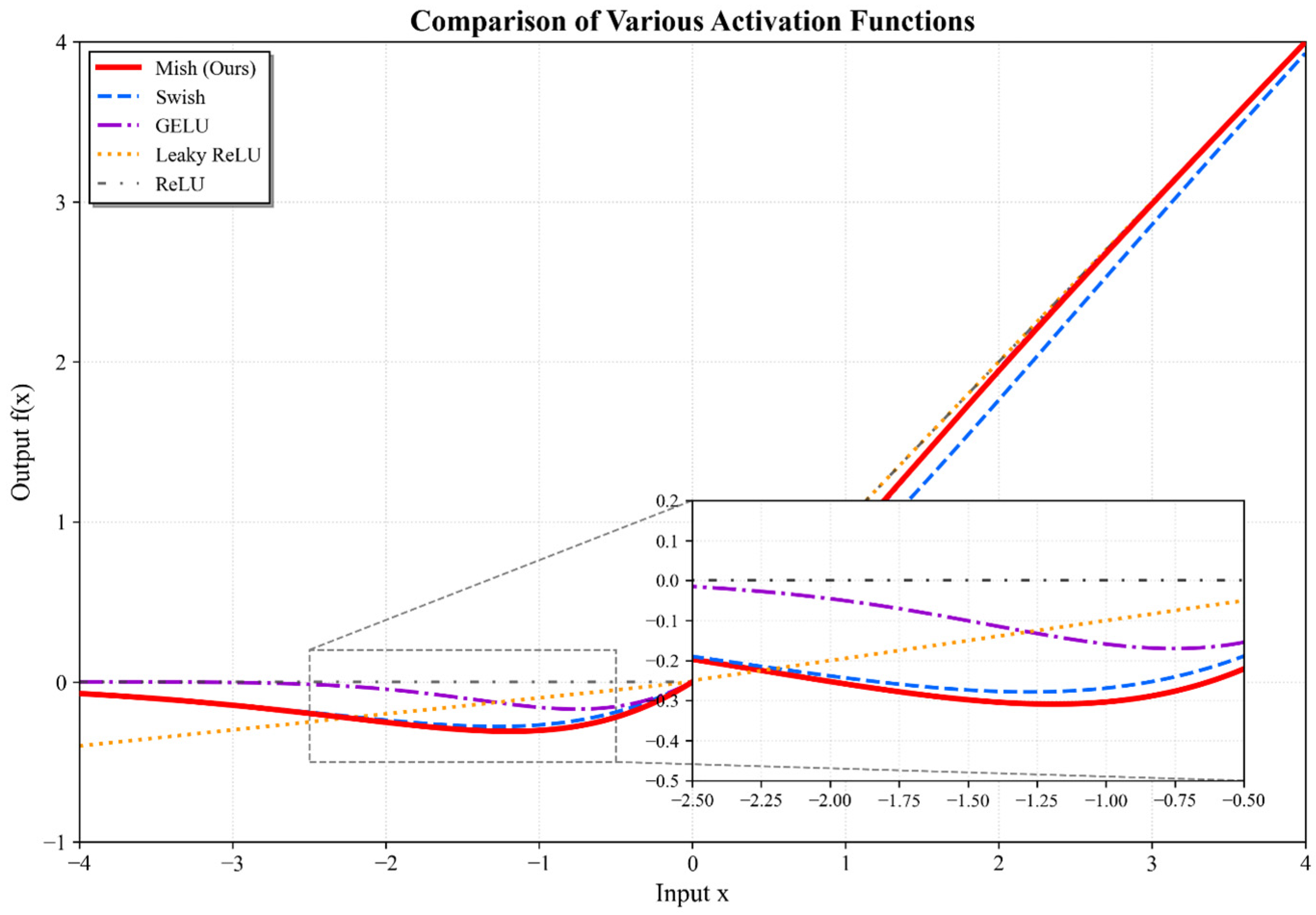
The Stem module first undergoes feature transformation via linear mapping to facilitate subsequent feature extraction. Unlike the traditional standard sequence of “Convolution-Normalization-Activation”, we place the BN layer before the 3 × 3 convolutional layer in this module. This design ensures that input features are standardized to a distribution with zero mean and unit variance before entering the convolution calculation, effectively mitigating the Internal Covariate Shift problem [48]. By allowing the convolutional kernels to learn on a more stable feature distribution, this strategy effectively accelerates the convergence speed of the model [48,49]. Furthermore, BN reduces gradient oscillations during deep network training, effectively lowering the model’s complexity without increasing the number of parameters, and ensures that the model can rapidly and stably extract low-level semantic information when processing HRRSIs with complex textures [50]. Finally, we select the Mish activation function to further ensure the smooth propagation of gradients and avoid the dying neuron phenomenon. As shown in Figure 5, we compare Mish with mainstream activation functions. Unlike the linear characteristics of ReLU and Leaky ReLU, Mish exhibits smoother non-monotonic properties in the negative region. Although Swish and GELU possess similar smooth curves, Mish has a deeper concave interval on the negative semi-axis (as shown in the magnified area in the figure), meaning it can better preserve minute negative gradient information, thereby enhancing the gradient flow and regularization effects of deep networks during training.

3.3. Multi-Branch Dilated Feature Extraction (MDFE) Module

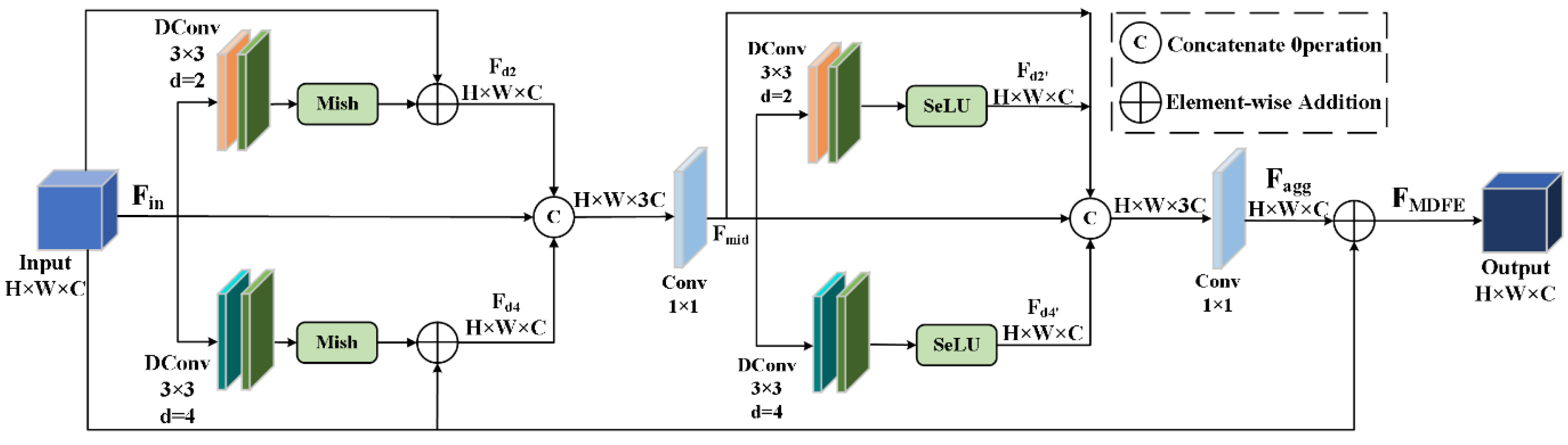
The MDFE module is shown in Figure 6, and its formulas are as follows:
F d 2 = M i s h D C o n v 3 × 3 d = 2 F i n + F i n
F d 4 = M i s h D C o n v 3 × 3 d = 4 F i n + F i n
F m i d = C o n v 1 × 1 C o n c a t F d 2 , F d 4 , F i n
F d 2 = S e L U D C o n v 3 × 3 d = 2 F m i d
F d 4 = S e L U D C o n v 3 × 3 d = 4 F m i d
F a g g = C o n v 1 × 1 C o n c a t F d 2 , F d 4 , F m i d
F M D F E = F a g g + F i n
where F i n R H × W × C represents the module input feature (the output of the previous layer), and D C o n v 3 × 3 d = k denotes a dilated convolution with a kernel size of 3 × 3 and a dilation rate of k . F d 2 and F d 4 represent the branch features of the first stage with dilation rates of 2 and 4, respectively, where local residual connections are introduced. C o n c a t denotes the concatenation operation along the channel dimension, and F m i d represents the intermediate feature of the first stage that fuses each branch and the original input. S e L U stands for the SeLU activation function, and F d 2 and F d 4 denote the branch features after SeLU activation in the second stage, respectively. C o n v 1 × 1 refers to a standard 1 × 1 convolution used for channel dimensionality reduction and feature fusion, F a g g indicates the aggregated feature of the second stage, and F M D F E is the final output feature of the MDFE module after a global residual connection.
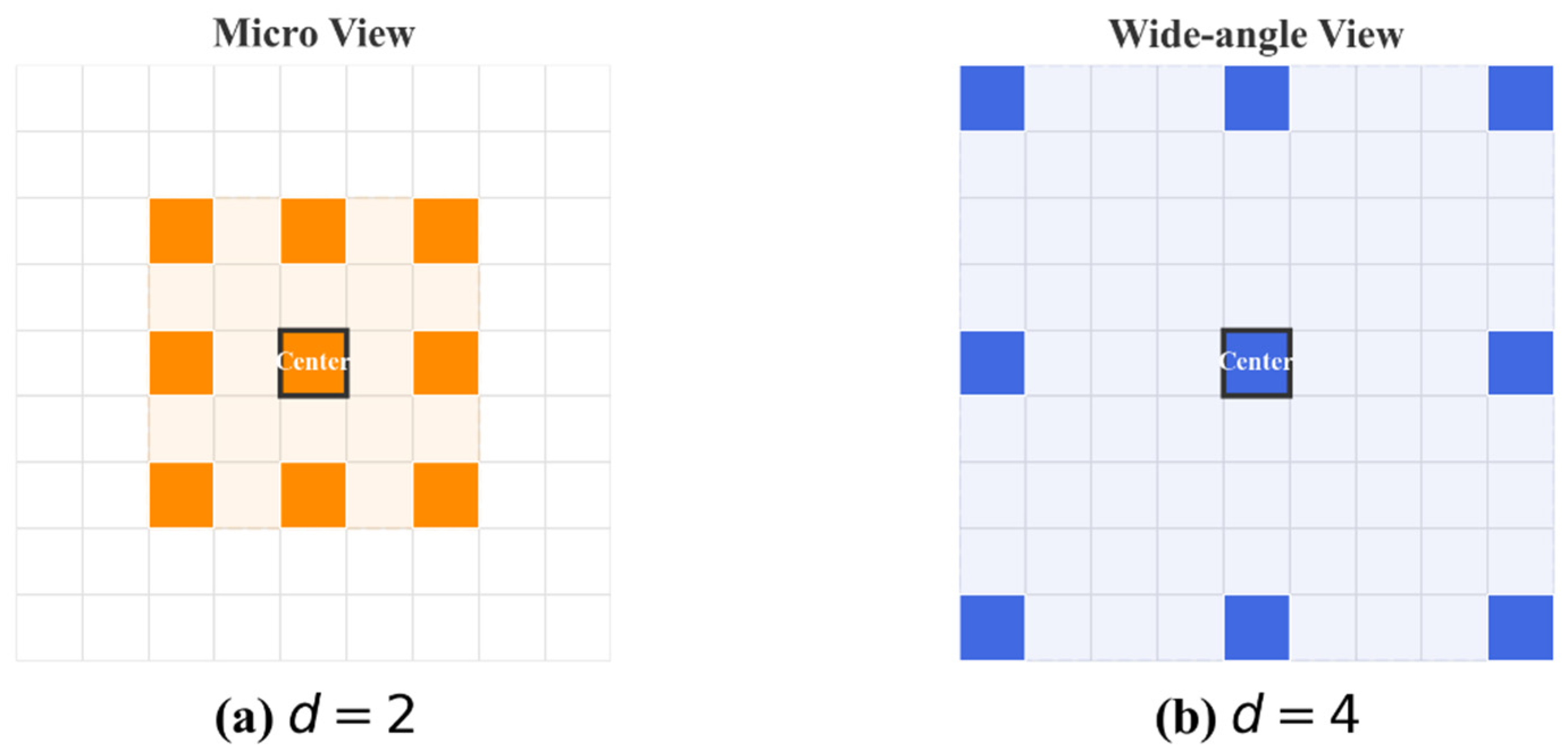
Traditional feature extraction units typically rely on fixed-size convolutional kernels, making it difficult for the model to simultaneously balance the global geometric structure of large-scale targets and the fine-grained textures of small-scale targets at the same hierarchical level. To break through this bottleneck, we designed the MDFE module, which adopts a dual-branch parallel architecture similar to a “zoom lens”. In MSALNet proposed by Yang et al. [51], an adaptive learning strategy is utilized to dynamically adjust the weights of multi-scale features to cope with scale effects in high-resolution remote sensing scenes. Unlike their scheme which focuses on weight adjustment, our MDFE module actualizes this concept structurally: we duplicate the complete input feature map into two parallel paths with specific dilation rates (as shown in Figure 7). Among them, the branch with d = 2 acts as a “macro lens,” focusing on capturing local textures and edge details of ground objects; meanwhile, the branch with d = 4 acts as a “wide-angle lens,” covering the complete geometric structure of large-scale targets like runways and rivers by expanding the receptive field. This parallel design ensures that local and global information is explicitly extracted separately, and then multiscale complementarity is achieved through concatenation operations, thereby avoiding information loss under a single scale.
To further enhance the nonlinear discriminative power of features, we introduce a mixed activation strategy within the MDFE module. As confirmed by Zhang et al. [52] in their research on hyperspectral image classification, adopting a hybrid depth-wise separable convolution and dual-branch feature fusion architecture can effectively enhance the network’s ability to capture subtle feature differences. Inspired by this, we deployed specific activation functions at different stages of MDFE to optimize gradient flow. Specifically, during the first stage of feature extraction, we utilize the Mish function, leveraging its smooth, non-monotonic properties to facilitate the effective propagation of deep gradients, preventing feature information from being lost during preliminary extraction. After feature fusion in the second stage, we switch to the SeLU function, utilizing its self-normalizing attribute to constrain the variance of the feature distribution post multi-branch fusion. This mixed strategy of “guiding propagation first, stabilizing distribution later” enables the network to learn compact and highly discriminative feature representations even with limited samples, thereby enhancing the training stability of the model while maintaining high classification accuracy.

3.4. Context-Position Aware Attention (CPAA) Module

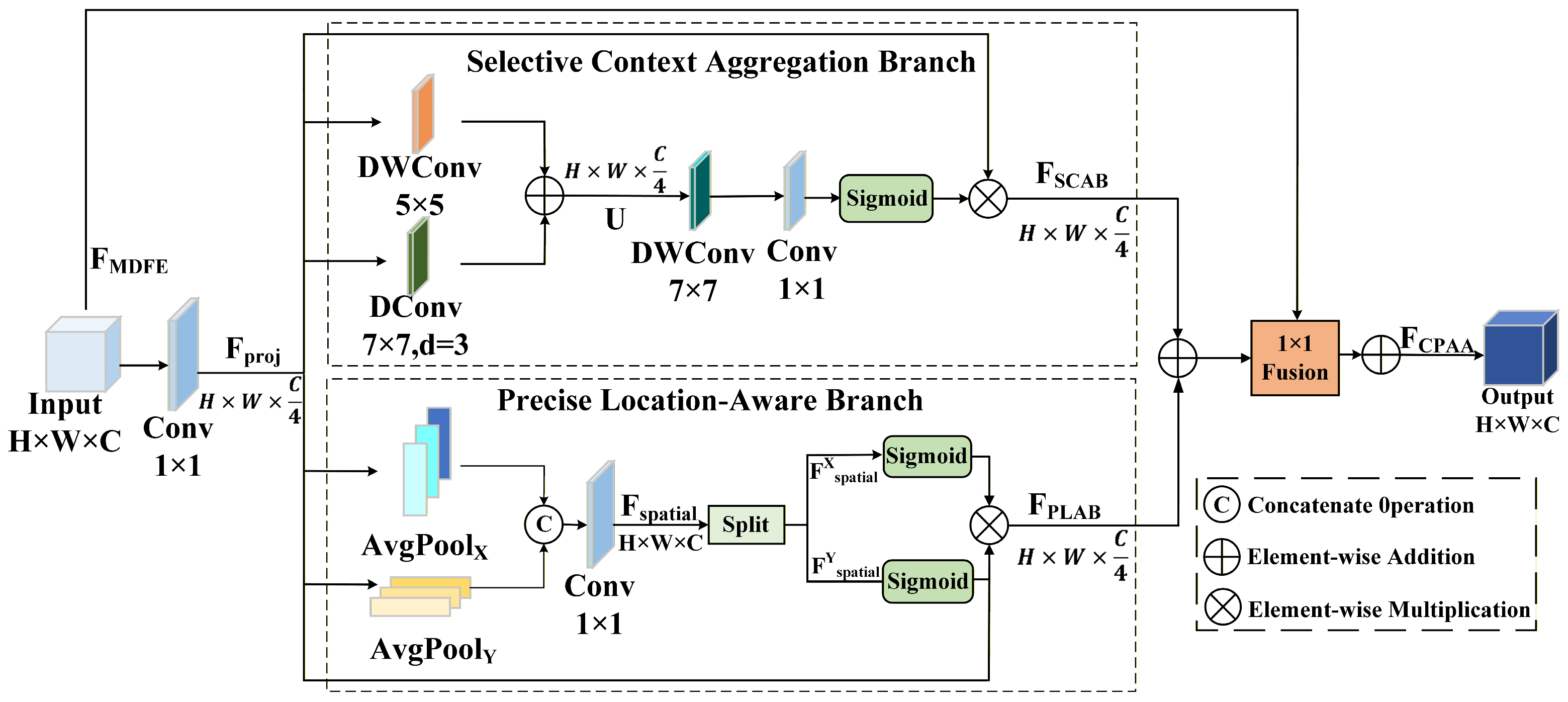
The structure of the CPAA module is shown in Figure 8, and its formulas are as follows:
F p r o j = C o n v 1 × 1 F M D F E
SCAB (11)–(12):
U = D W C o n v 5 × 5 F p r o j + D C o n v 7 × 7 d = 3 F p r o j
F S C A B = F p r o j S i g m o i d C o n v 1 × 1 D W C o n v 7 × 7 U
PLAB (13)–(15):
F s p a t i a l = C o n v 1 × 1 C o n c a t A v g P o o l X F p r o j , A v g P o o l Y F p r o j
F s p a t i a l X , F s p a t i a l Y = S p l i t F s p a t i a l
F P L A B = F p r o j S i g m o i d F s p a t i a l X S i g m o i d F s p a t i a l Y
F C P A A = C o n v 1 × 1 F S C A B + F P L A B + F M D F E
where F M D F E denotes the input feature of the CPAA module, and F p r o j represents the feature after projection and dimensionality reduction. D W C o n v 5 × 5 refers to a depth-wise separable convolution with a size of 5 × 5 , and D C o n v 7 × 7 d = 3 denotes a dilated convolution with a size of 7 × 7 and a dilation rate of 3. U represents the intermediate feature aggregating local and long-range contexts, S i g m o i d denotes the Sigmoid activation function, and represents element-wise multiplication. F S C A B signifies the context feature after background suppression, while A v g P o o l X and A v g P o o l Y denote GAP operations along the width and height directions, respectively. C o n c a t represents the concatenation operation, F s p a t i a l is the spatially encoded feature fused via 1 × 1 convolution, S p l i t indicates splitting the feature along spatial dimensions to obtain the horizontal and vertical spatial feature vectors, explicitly denoted as F s p a t i a l X and F s p a t i a l Y , respectively. F P L A B represents the feature enhanced by position awareness. F C P A A signifies the final output feature of the CPAA module after fusing the two branches and adding a global residual connection.
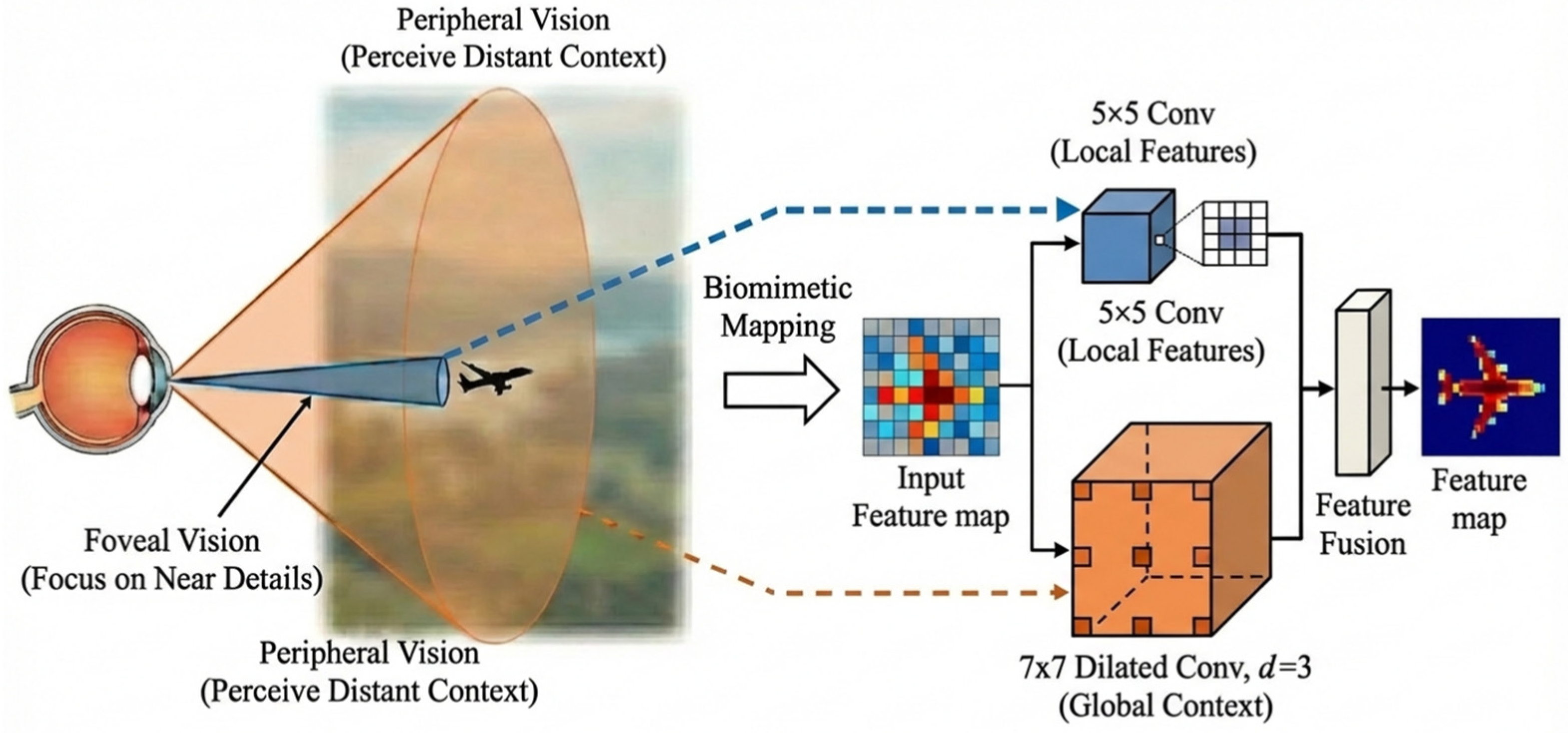
In complex remote sensing scenes, clouds, shadows, and task-irrelevant background textures often interfere with the model’s judgment. However, the human visual system exhibits exceptional efficiency when processing such complex scenes. As shown in Figure 9, human observation patterns feature a unique “selective attention” mechanism: when observing objects, we utilize foveal vision to clearly capture the fine-grained textures of nearby targets, while simultaneously employing peripheral vision to perceive the distant, broad environmental context. This dual-perception mode allows humans to naturally filter out background noise that is inconsistent with the current focal point. GACNet, proposed by Tan et al. [53], further verified the effectiveness of this bionic mechanism; by simulating the biological visual processes of saccades and fixation, this research constructed a global-local collaborative perception feature filter, effectively enhancing the model’s anti-interference capabilities in complex backgrounds.
Inspired by this, our SCAB abandons complex mathematical solvers and instead adopts an intuitive large-kernel decomposition strategy to simulate this “biological eye” mechanism. We utilize depth-wise separable convolutions of size 5 × 5 to simulate “central focus,” responsible for extracting the ontological features of the target; simultaneously, we incorporate 7 × 7 dilated convolutions with a dilation rate of 3 to simulate “peripheral perception,” expanding the effective receptive field to cover the background environment without increasing computational burdens. Through this mechanism, the model can function similar to a human eye, precisely locking onto local targets while confirming scene semantics via broad contextual information, thereby effectively suppressing irrelevant background interference and achieving robust feature extraction.
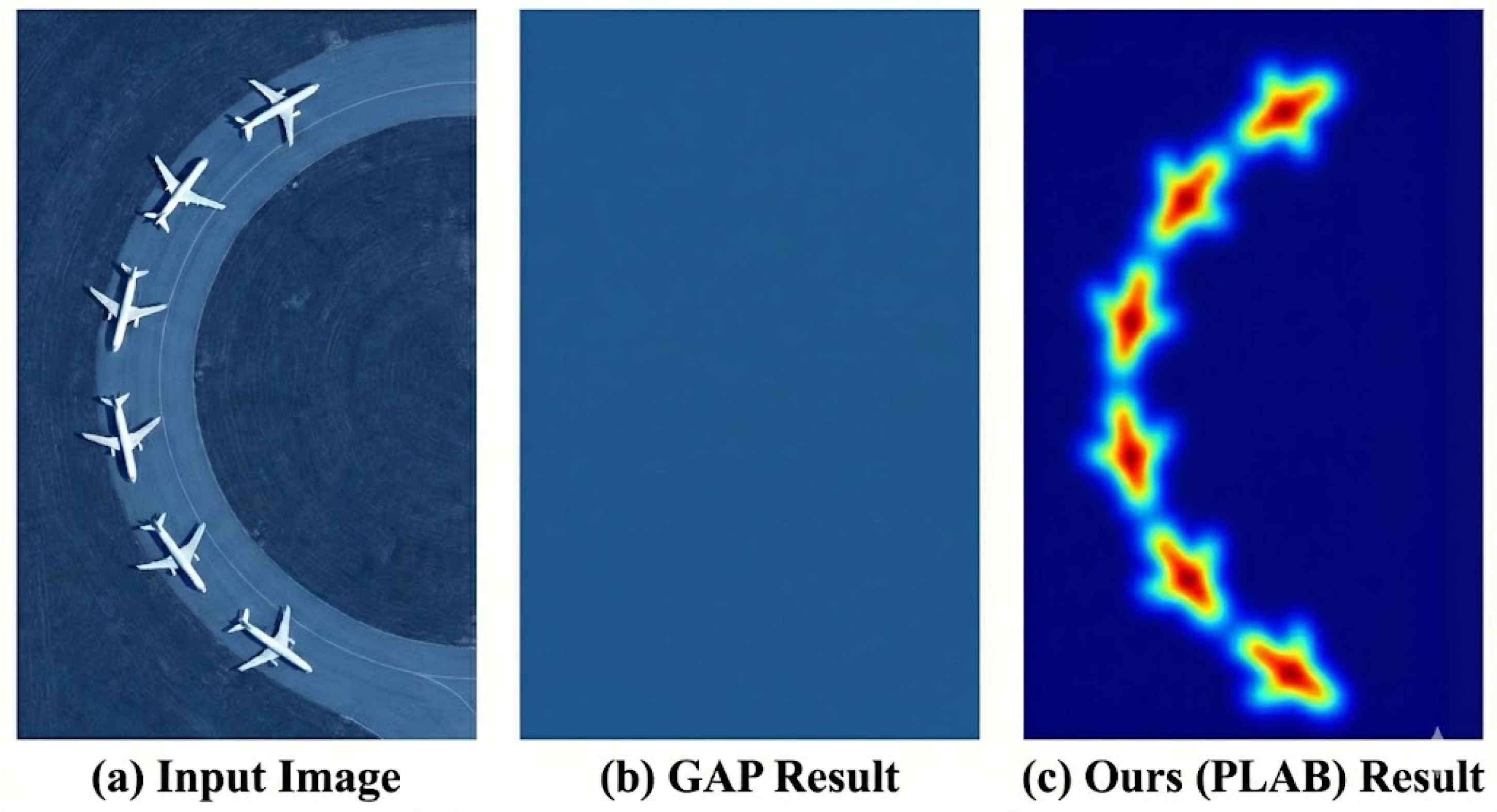
Moreover, traditional GAP compresses spatial dimensions into a single scalar, leading to the loss of crucial positional structural information, which is highly detrimental for distinguishing densely arranged scenes. SC-Net, proposed by Huang and Guo [54], emphasized the importance of preserving spatial geometric structures through directional feature decomposition, which plays a significant role in accurate modeling of cross-scale targets. To integrate this concept into our lightweight architecture, our PLAB branch discards direct global pooling and instead adopts a coordinate encoding mechanism. To verify the effectiveness of this mechanism in processing complex ground object distributions, we showcase the feature extraction visualization results of our model in Figure 10. As depicted in Figure 10b, when facing airplane targets densely arranged diagonally on an apron, standard GAP operations forcefully compress two-dimensional features into a single value, causing a complete collapse of the “airplane’s” spatial structural information, rendering the model unable to perceive the specific distribution pattern of the targets. Conversely, as shown in Figure 10c, our PLAB branch aggregates features along horizontal and vertical directions separately, generating a pair of direction-aware vectors containing precise coordinate information. When these two vectors are reconstructed back into two-dimensional space via an outer product, they exhibit a clear positioning response, accurately locking onto the coordinate locations of all airplanes. This mechanism ensures the model remains highly sensitive to the spatial distribution of ground objects, thereby maintaining outstanding classification performance even when confronted with densely arranged small targets.
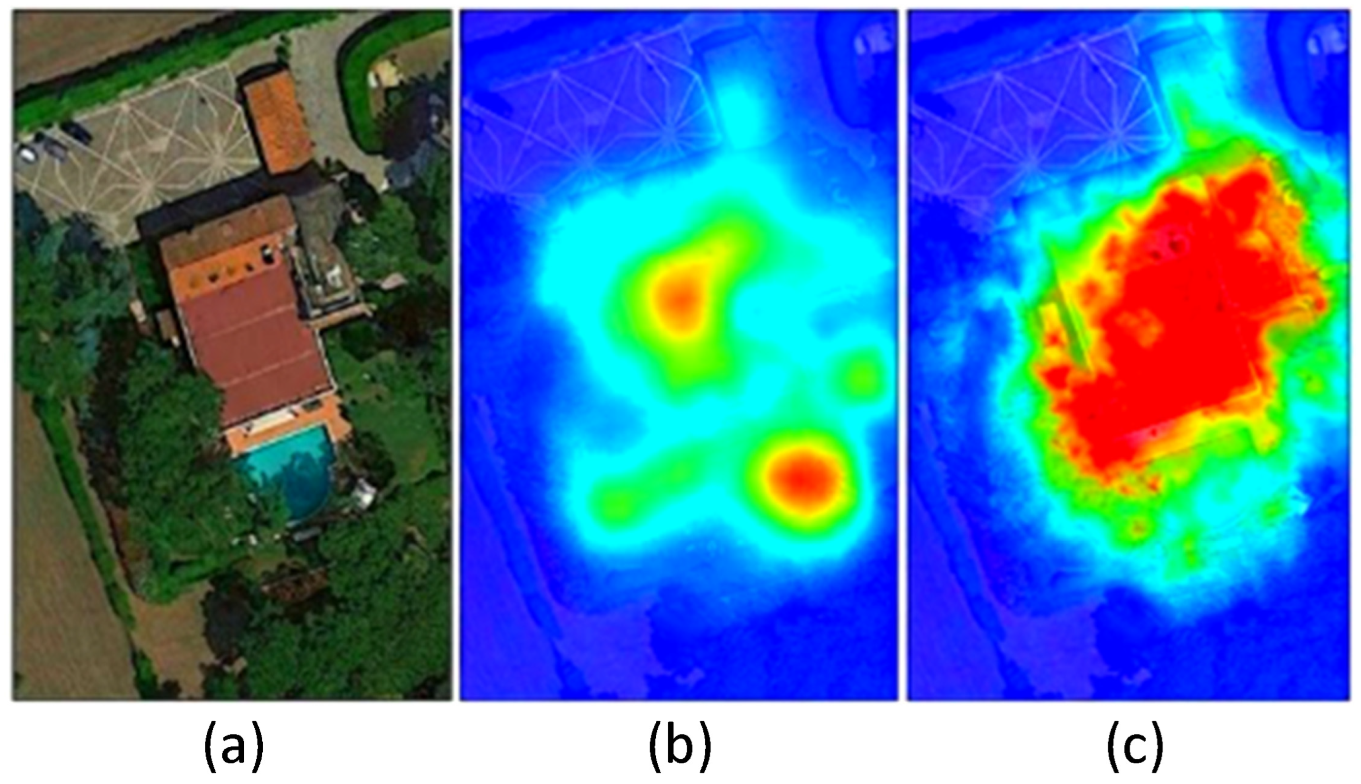
Furthermore, to intuitively demonstrate the overall effectiveness of the Context-Position Aware Attention (CPAA) module in handling complex background clutter, we employed the Grad-CAM algorithm to visualize the class activation maps. Figure 11 presents a visual comparison using a representative “SparseResidential” sample.
As observed in Figure 11b, the baseline network lacking the CPAA mechanism exhibits a relatively dispersed attention distribution. The high-response regions are easily distracted by surrounding environmental interference, improperly allocating attention to background elements such as swimming pools, rather than focusing entirely on the defining residential structures.
Conversely, upon integrating the CPAA module (Figure 11c), the network’s attention becomes significantly more concentrated. Driven by the synergistic effects of the selective context aggregation and precise location awareness, the model demonstrates an improved capability to suppress irrelevant background noise. The primary activation areas (indicated by the intense red regions) more precisely encapsulate the main architectural targets. This visual evidence further substantiates that the CPAA module assists the network in anchoring on discriminative foreground features, thereby enhancing classification robustness in complex remote sensing scenes.

3.5. Loss Function Optimization

To improve the model’s generalization capabilities in complex remote sensing scenes and prevent overfitting, we adopted a label smoothing regularization strategy to optimize the objective function, with formulas as follows:
y L S , k = 1 ϵ y k + ϵ K
L t o t a l = k = 1 K y L S , k log p k = k = 1 K 1 ϵ y k + ϵ K log p k
where y L S , k represents the smoothed soft label, ϵ is the smoothing hyperparameter (set to 0.1 in this experiment), and y k is the ground truth label indicator (1 if the sample belongs to class k , 0 otherwise). K denotes the total number of scene categories, L t o t a l indicates the final total loss value, and p k is the predicted probability distribution output by the network.
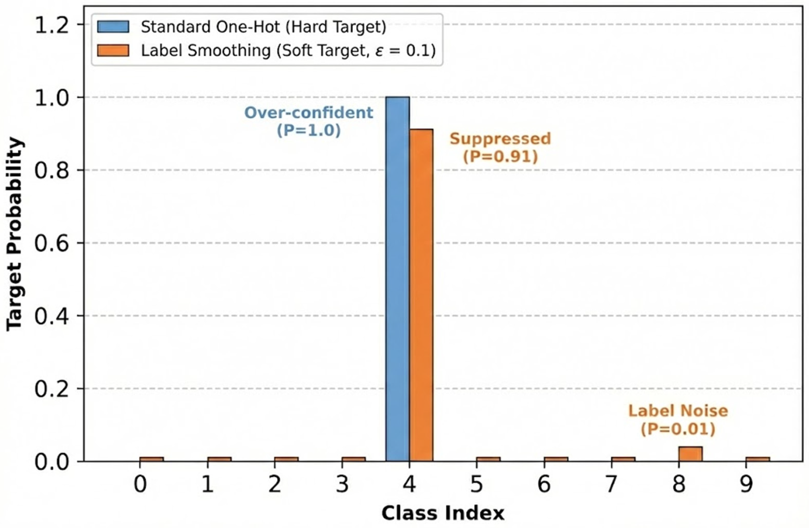
During the model training phase, the standard Cross-Entropy (CE) loss function typically relies on “Hard” One-Hot Encoding. As shown in Figure 12, this encoding scheme forces the model to push the predicted probability of the target class to an extreme 1.0, while completely suppressing non-target classes to 0. Such a strong supervision signal often causes the model to become over-confident in the later stages of training, leading to overfitting when faced with ambiguous samples near decision boundaries [55]. To mitigate this issue, we introduce a label smoothing strategy [56]. By incorporating the hyperparameter ϵ , the originally sharp probability distribution is effectively “smoothed,” suppressing the upper limit of the true class confidence to 1 ϵ , while assigning a uniformly small probability value of ϵ / K to the remaining non-true classes. This mechanism is equivalent to introducing controllable background noise into the training objective; it no longer demands absolute certainty in predictions but rather encourages the network to learn feature clusters that are more compact intra-class and possess clearer inter-class boundaries within the feature space. Experiments demonstrate that this “softening” label regularization method effectively smooths decision boundaries, significantly enhancing the model’s robustness against label noise and inter-class confusion.

4. Experiments

4.1. Datasets

To comprehensively verify the feasibility and effectiveness of the proposed model, we conducted extensive experiments on three challenging public remote sensing scene datasets, including the Aerial Imagery Dataset (AID) [9], NWPU-RESISC45 (NWPU45) [1], and RSD-WHU46 [57,58]. Table 1 lists the relevant information and training ratios of the aforementioned datasets. Among them, NWPU45 is a strictly class-balanced dataset, whereas AID and RSD-WHU46 exhibit typical class imbalance and long-tail distribution characteristics. For instance, in the RSD-WHU46 dataset, “regular farmland” contains up to 3000 images, while “medium density scattered building” contains only 500 images. This easily leads to prediction preferences in the model and poses stringent requirements on network robustness.
The aforementioned datasets are not only massive in scale but also contain extremely rich scene categories. Some scenes of different semantic categories exhibit minute visual differences, while scenes of the same category show significant appearance variations due to changing imaging conditions. Furthermore, as the most representative large-scale datasets in the current RSSC field, the HRRSIs in NWPU45 and RSD-WHU46 are sourced from various sensors and feature extremely complex spatial layouts. The high similarity of these target objects in geometric structure and spectral response further increases the difficulty of scene classification. Finally, to effectively mitigate overfitting and further enhance the model’s generalization capability, we applied data augmentation techniques to the training dataset during the training phase, including horizontal and vertical flipping, as well as adaptive brightness adjustment.

4.2. Experimental Parameters and Evaluation Metrics

All our experiments were implemented using the PyTorch 2.8.0 deep learning framework [59] on a server running the Linux operating system. The hardware configuration included a high-performance CPU, 90 GB of memory, and an NVIDIA RTX 5090 (32 GB) GPU for acceleration. The detailed software and hardware environment configurations and hyperparameter settings are presented in Table 2. Regarding the training strategy, we utilized the Stochastic Gradient Descent (SGD) optimizer with a momentum of 0.9 and a weight decay of 5 × 10 4 to optimize network parameters. The initial learning rate was set to 2 × 10 5 , the batch size to 16, and the training process spanned 200 epochs. To prevent gradient explosion during deep training, we set the gradient clipping threshold to 5.
To ensure reproducibility and fair comparison, we standardized the experimental pipeline. Specifically, input images from the NWPU-RESISC45 and RSD-WHU46 datasets were resized to 256 × 256, while images from the AID were resized to 600 × 600. These images were processed using random cropping during training and center cropping during testing. We applied standard color normalization (mean = [0.485, 0.456, 0.406], std = [0.229, 0.224, 0.225]). The random seed was fixed at 42 across all experiments. Network weights were initialized using Kaiming initialization. We adopted a Cosine Annealing learning rate schedule with a 5-epoch linear warmup, and no early stopping was used to allow full convergence over 200 epochs.
To comprehensively quantify the classification performance and computational efficiency of the model, we adopted the following evaluation metrics:
  • Overall Accuracy (OA): Measures the proportion of correctly classified samples over the total samples in the test set, reflecting overall performance.
  • Confusion Matrix: Used to visualize the classification results for each category and analyze inter-class confusion.
  • Precision, Recall, and F1-Score: Used to analyze the classification performance of the model on individual categories.
  • Parameters and GMACs (Giga Multiply–Accumulate Operations): Used to evaluate the spatial and time complexities of the model, verifying its deployment potential in resource-constrained environments.

4.3. Experimental Results

4.3.1. Experimental Results on the AID

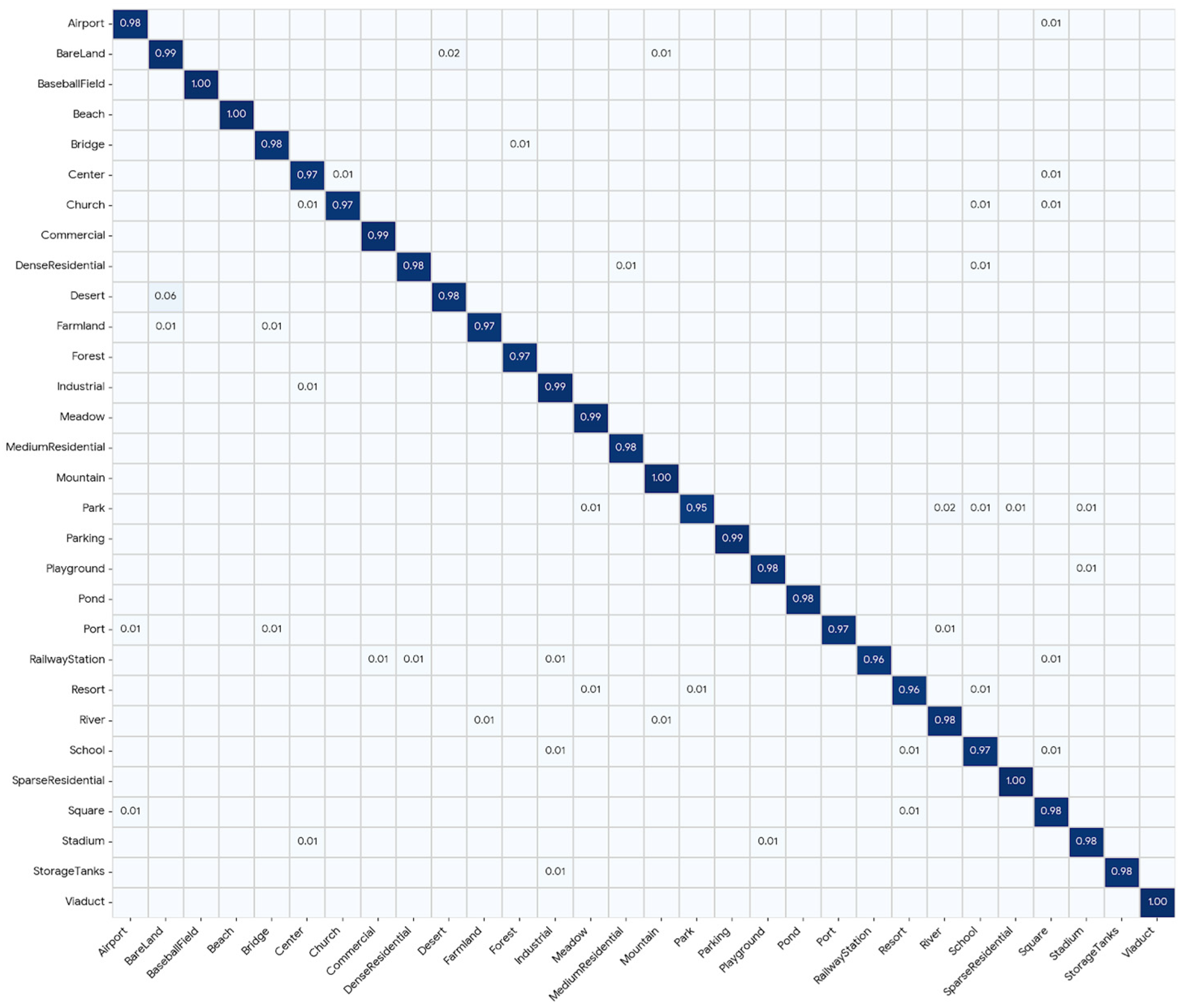
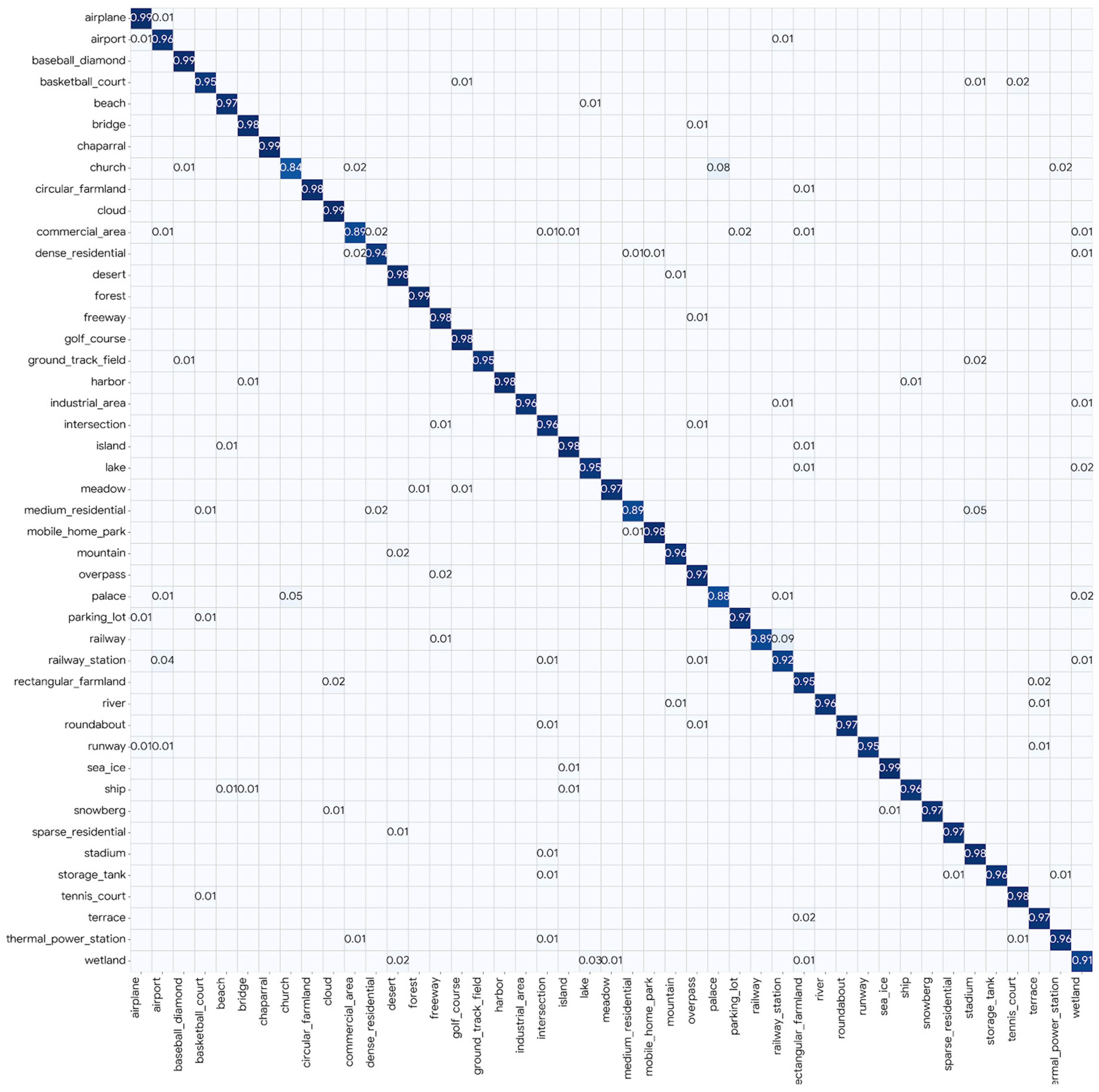
The following are the experimental results on the AID. Table 3 presents the classification accuracy (OA) of our proposed MS-DARNet compared with other models. To provide a more detailed performance evaluation, Table 4 summarizes the specific evaluation metrics for each individual category, including precision, recall, and F1 score. Additionally, Figure 13 displays the confusion matrix.
From Table 3 and Table 4, and Figure 13, we observe the following:
  • Improved ACC: We can observe from Table 3 that, under a 50% training ratio, our proposed MS-DARNet achieved an accuracy of 97.78%, which is a 1.43% and 0.80% improvement over the classic model ResNet50 (96.35%) [64] and the SOTA model LG-DCN (96.98%) [49], respectively. When dealing with complex remote sensing scenes, classic networks (such as ResNet50) fail to effectively extract target objects of varying scales, potentially leading to insufficient feature learning. For instance, when recognizing a “Parking” scene, the network requires both a small receptive field to precisely extract the local fine-grained features of tiny “cars” and a massive receptive field to perceive the global spatial layout of the entire parking lot. The fixed standard convolutional kernels of ResNet50 struggle to balance these two extreme-scale pieces of information simultaneously at the same feature level, making it prone to losing critical features. To effectively handle target objects of different scales, LG-DCN proposed a dynamic convolutional framework based on a distribution-collaboration strategy, aiming to dynamically generate convolutional weights by extracting global channel descriptors. However, this method, which is highly dependent on global feature compression, inevitably leads to the loss of critical spatial coordinates and local geometric structural information. In contrast, our model naturally achieves dynamic expansion of the receptive field through the parallel dilated branches of the MDFE module. Furthermore, the CPAA module abandons extreme spatial feature compression mechanisms. Through a more refined feature aggregation strategy, it effectively filters background noise while maintaining high spatial resolution responses, thereby improving classification accuracy.
  • Enhanced Ability to Recognize Fine-grained Categories: The detailed evaluation metrics in Table 4 further reflect the model’s classification performance across various categories. In recent years, to improve the extraction capability of complex fine-grained features in remote sensing images, many studies have widely introduced attention mechanisms [69]. For example, some advanced methods based on traditional CNNs integrate channel and conventional spatial attention modules to enhance focus on key features, while Transformer-based networks (such as STMSF) utilize self-attention mechanisms for global information interaction and modeling. However, most existing attention mechanisms still exhibit obvious limitations when processing fine-grained categories with significant spatial geometric distribution characteristics. To reduce computational dimensionality, such methods generally rely on conventional GAP operations at the network’s end, forcibly compressing two-dimensional spatial dimensions into a single numerical value. This processing inevitably leads to the collapse and loss of the critical positional coordinate information of targets, severely restricting the model’s spatial structure parsing capability for densely arranged scenes (such as vehicles in a parking lot). By comparison, the PLAB mechanism in our CPAA module effectively overcomes this flaw of conventional attention mechanisms. Unlike traditional operations that directly perform spatial dimensionality reduction, PLAB discards brute-force global spatial compression and aggregates features along horizontal and vertical directions separately via a direction-aware vector extraction mechanism. As shown in Figure 10, this unique mechanism can clearly locate the absolute positions of targets during feature reconstruction, thereby explicitly and precisely preserving spatial coordinate information within the attention feature map. Thanks to this high sensitivity to the spatial layout of dense objects, the model performs more stably on fine-grained categories. For instance, on the “Parking” and “Meadow” categories, the model achieved 100% precision or recall. Furthermore, when facing complex background fine-grained scenes such as “BaseballField” (F1 score of 98.87%) and “Commercial” (F1 score of 98.72%), PLAB’s precise coordinate preservation capability allows the model to effectively distinguish subtle feature differences, resulting in higher classification accuracy.
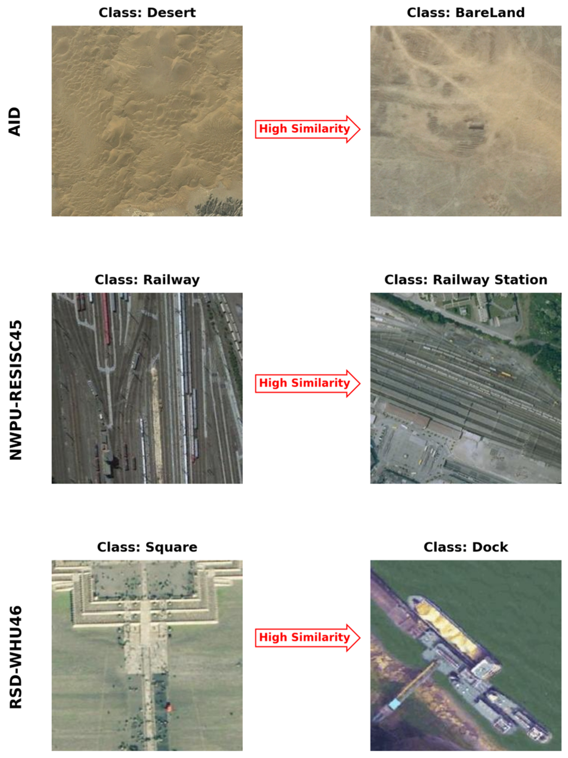
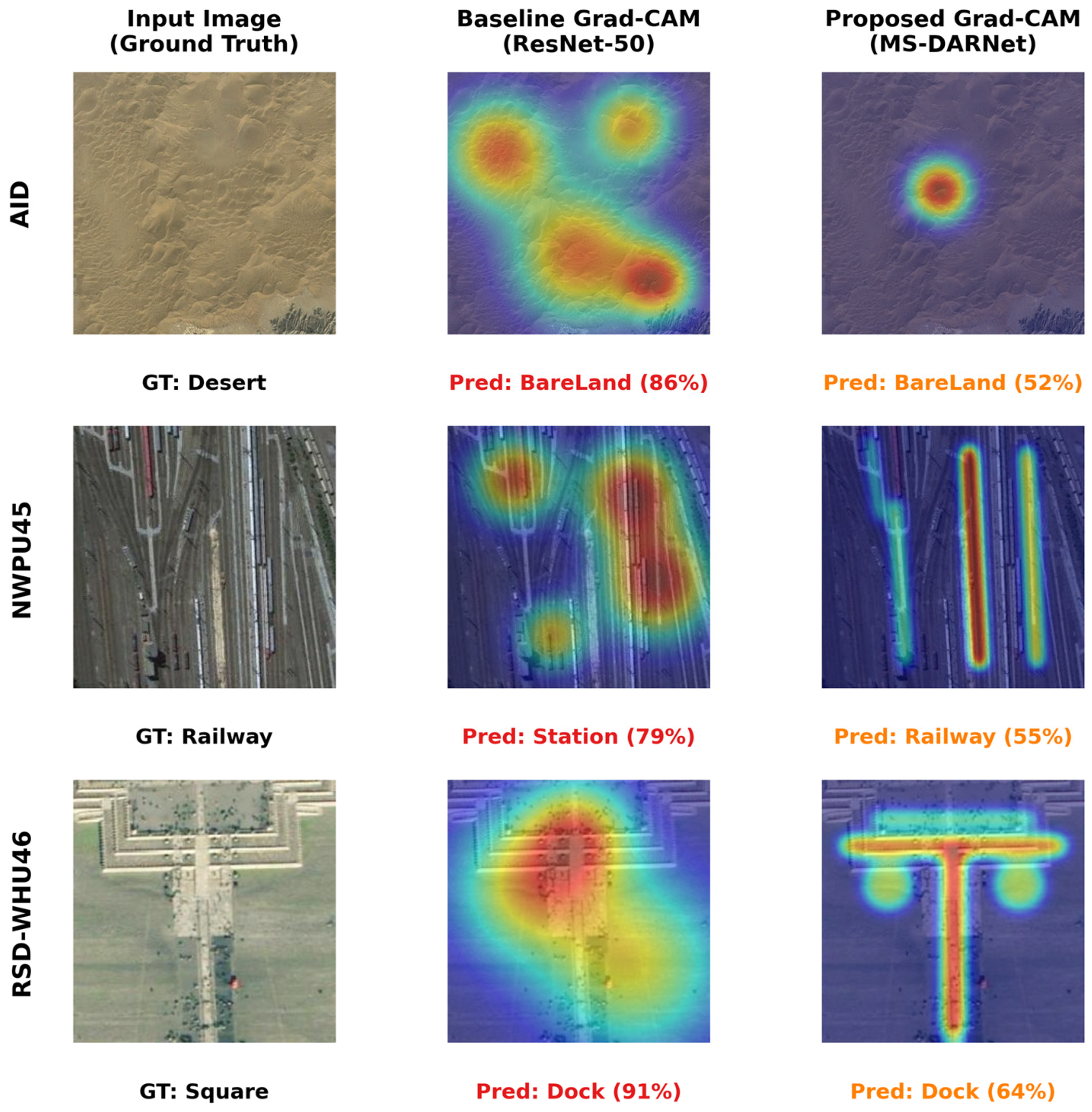
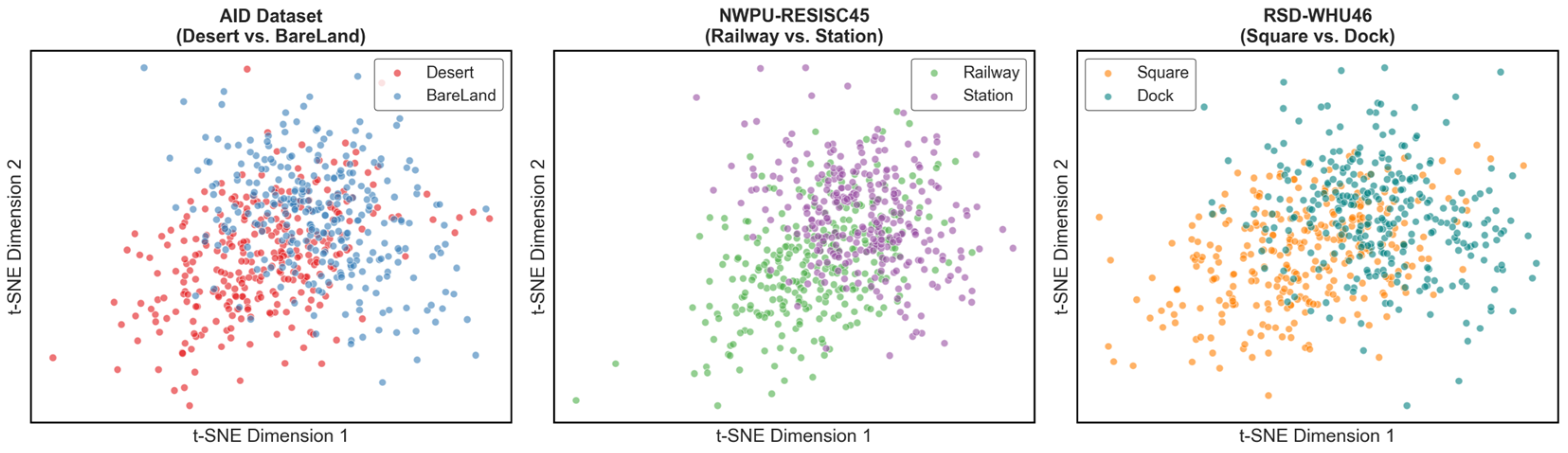
  • Reduced Inter-class Misclassification Rate: The confusion matrix in Figure 13 provides an intuitive demonstration of the model’s discriminative ability. The dark regions along the diagonal indicate that the model makes correct predictions for the vast majority of categories. For instance, the classification accuracies for natural scenes like “Beach” and “Forest” reached 1.00 and 0.99, respectively. Although densely built scenes such as “School” and “Commercial” are visually extremely similar and prone to misjudgment, our model restricts their confusion rate to a very low range (only 0.01). This is attributed to the “macro” and “wide-angle” dual-branch design of the MDFE module, which enables the model to simultaneously utilize local texture details and global spatial layouts to distinguish scenes with similar appearances but different semantics, achieving precise differentiation of similar scenes. However, an analysis of the confusion matrix also reveals that the model still possesses certain limitations when confronting specific scenes lacking significant structural features and sharing highly similar textures. For example, 6% of the samples in the “Desert” category were incorrectly classified as “BareLand”. This is primarily because these two scenes are extremely similar in physical attributes, spectral features, and underlying textures, and they lack regular geometric structures (such as building edges or road networks) to serve as effective directional coordinate information for the PLAB branch. In such cases, even if the SCAB can perceive a wide range of global contexts, the model still struggles to classify targets accurately due to the lack of local structural anchors with strong discriminative power. This indicates that while our model performs excellently in structured scenes containing complex spatial layouts, the robustness of its feature extraction requires further improvement in future work when processing natural ground objects with extremely high similarity and no obvious boundaries.

4.3.2. Experimental Results on the NWPU-RESISC45 Dataset

The following are the experimental results on the NWPU-RESISC45 dataset. Compared to the aforementioned AID, the NWPU-RESISC45 dataset not only contains more scene categories and a larger data scale but also exhibits higher visual similarity among different scene categories (such as “Palace” and “Church”). Scenes of the same category also present massive appearance differences due to changes in imaging conditions like illumination and seasons, posing a more severe test on the generalization and anti-interference capabilities of feature extraction networks. Table 5 shows the OA comparison between our proposed MS-DARNet and other models. To provide a finer performance evaluation, Table 6 summarizes the detailed evaluation metrics for each individual category under this dataset, including precision, recall, and F1 score. In addition, Figure 14 displays the confusion matrix.
From Table 5 and Table 6, and Figure 14, we observe:
  • Improved ACC: From Table 5, we can observe that under a 20% training ratio, our proposed model achieved an accuracy of 94.53%. Compared with the advanced model LG-MSMA (94.17%) [50] proposed in 2025, our model’s accuracy increased by 0.36%. When coping with complex remote sensing scenes, traditional classic networks usually rely on fixed feature extraction structures, struggling to adaptively handle drastic scale variations in ground objects. To enhance the network’s perception of multi-scale features, advanced models represented by LG-MSMA introduced multi-scale feature fusion and mixed attention mechanisms. However, when calculating attention weights, such methods not only bring high mathematical and computational complexity but their conventional spatial attention mechanisms also often lack the effective capture and explicit filtering capabilities for broad contextual environments when confronting the extremely complex background interference in the NWPU-RESISC45 dataset. Our model does not rely on highly computational mathematical methods but constructs a direct environmental perception paradigm based on a pure convolutional framework. By explicitly decoupling multi-scale receptive fields and the aggregation of broad contexts within the same network level, MS-DARNet enables the model to adaptively isolate highly discriminative target features from highly similar redundant backgrounds while maintaining high computational efficiency. This lightweight and intuitive architectural design effectively avoids the information distortion problems caused by complex mathematical mapping, thereby achieving superior overall classification performance in extremely challenging high-noise datasets.
  • Enhanced Capability to Extract Contextual Feature Information: Table 6 demonstrates the model’s classification robustness across various categories. To address the complex background interference in the NWPU-RESISC45 dataset, LSMNet proposed by Zhang et al. [41] introduced extremely large convolutional kernels (such as 21 × 21) to break the physical limitations of traditional receptive fields, aiming to capture the broad global context environment. However, this singular oversized kernel design lacks refined spatial selectivity. When faced with the highly complex macroscopic backgrounds in this dataset, a massive receptive field can easily indiscriminately mix irrelevant environmental noise with core target features, leading to the dilution of discriminative information and inter-class confusion. To effectively overcome this problem, the SCAB in our proposed CPAA module plays a crucial role. Instead of blindly enlarging a single convolutional kernel, the SCAB adopts a bionic large-kernel decomposition strategy (combining 5 × 5 convolutions and 7 × 7 dilated convolutions with a dilation rate of 3). This mechanism utilizes 5 × 5 convolutions to precisely focus on and extract the target’s ontological local features, while simultaneously using parallel dilated convolutions to independently and effectively aggregate long-range global context information. Through this explicit decoupling, the model naturally filters out background noise that is inconsistent with the current focal point. Therefore, the model performs excellently on categories with distinct features; for instance, it achieved 100% precision on the “Chaparral” category and a 98.86% recall on the “Sea Ice” category. Even for artificial scenes like “Church” and “Palace”, which possess highly similar architectural styles and are easily interfered with by complex surrounding environments, the model maintains a high recognition capability. This demonstrates that our model can suppress background noise by effectively extracting and understanding broader contextual information, thereby improving classification performance in complex scenes.
  • Enhanced Anti-Background Noise Interference Capability: The confusion matrix in Figure 14 further intuitively demonstrates the model’s discriminative ability. The dark areas on the diagonal indicate that the model can make correct predictions for the vast majority of categories. For instance, the classification performance for scenes such as “SeaIce” and “Chaparral” is exceptional. Traditional models often struggle to distinguish scenes with similar geometric structures, but as shown in Figure 14, our model effectively reduces confusion between scenes with similar semantics through its large-kernel context aggregation mechanism. This outstanding discriminative ability is attributed to the SCAB module, which helps the model extract the target’s ontological features while effectively suppressing the interference of background noise, thereby achieving precise differentiation of similar scenes. However, an in-depth analysis of the confusion matrix also reveals that the model has certain limitations when processing scenes with highly overlapping local features. For instance, 9% of the samples in the “Railway” category were misclassified as “Railway Station”. This is primarily because these two scenes often share the same macroscopic context in reality (such as stretching tracks and surrounding industrial facilities). In this scenario, the broad background information extracted by the SCAB is difficult to use as an effective discriminative basis to distinguish the two. If the core building of the “Railway Station” (such as platforms or canopies) is too small in scale or its features are not salient enough in the image, the model struggles to complete precise classification relying solely on faint ontological features. This indicates that although our model effectively filters irrelevant background noise, its ability for fine-grained feature decoupling requires further improvement in future work when confronted with scenes where the background environment is highly consistent and the core differences are extremely minimal.

4.3.3. Experimental Results on RSD-WHU46

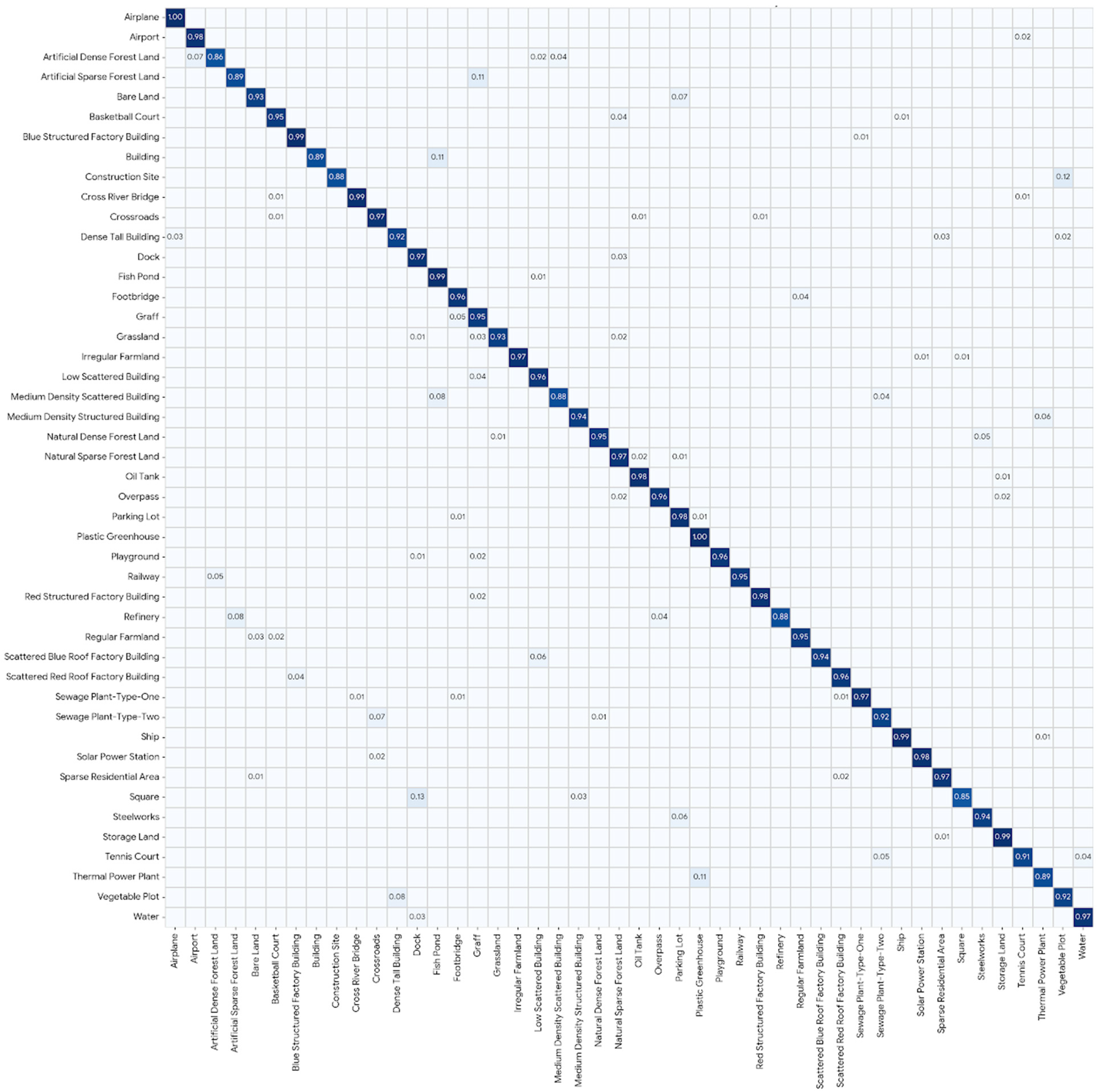
The following are the experimental results on the RSD-WHU46 dataset. Compared with AID and NWPU-RESISC45, the RSD-WHU46 dataset presents a higher classification difficulty. Its data scale is more massive, and it is a typical class-imbalanced dataset. Furthermore, this dataset contains a large number of complex categories with highly overlapping semantics (such as different types of farmlands and various forms of factory buildings). This extreme long-tail distribution superimposed on minute fine-grained differences places higher demands on the model’s generalization and feature extraction capabilities. Table 7 shows the OA of our proposed MS-DARNet and other models. To provide a more detailed performance evaluation, Table 8 summarizes the detailed evaluation metrics for each individual category, including precision, recall, and F1 score. Additionally, Figure 15 displays the confusion matrix, visualizing the model’s discriminative performance across all 46 categories.
From Table 7 and Table 8, and Figure 15, we find:
  • Improved ACC: From Table 7, we can observe that under a 20% training ratio, MS-DARNet achieved an accuracy of 94.55%. Compared to the SOTA model CLGDL (94.21%) [52], our model’s accuracy improved by 0.34%. Faced with massive and unevenly distributed remote sensing images, CLGDL introduced a multi-layer heterogeneous feature fusion mechanism combining Lie group machine learning and deep learning. However, when mapping features to non-Euclidean Lie group manifolds, such methods typically rely heavily on global feature statistical aggregation (such as covariance matrix computation or global pooling). This processing is very prone to forcibly mixing targets with the surrounding complex macroscopic backgrounds when confronting the tiny objects with diverse shapes and dense arrangements in RSD-WHU46, resulting in the irreversible loss of critical spatial details. By comparison, our MS-DARNet introduces a Bionic Selective Perception mechanism. The model abandons brute-force global spatial compression and explicitly decouples the local ontological features of the target from the long-range global context via a large-kernel decomposition strategy. This mechanism enables the model to act like the human visual system, precisely “focusing” on targets and filtering irrelevant noise within vast complex backgrounds. Consequently, it exhibits exceptional anti-interference capabilities when processing the extremely complex spatial layouts of RSD-WHU46, achieving higher classification precision.
  • Precise Decoupling Capability for Easily Confused Categories: From Figure 15 and Table 8, we find that the model performs excellently when processing complex agricultural and industrial categories with highly overlapping semantics. RSD-WHU46 contains many highly confusable fine-grained categories (such as “Plastic Greenhouse” and “Regular Farmland”). To distinguish these scenes, the two-stream architecture SDLS [24] proposed by Ma et al. attempts to introduce self-distillation mechanisms and local feature streams to strengthen the capture of discriminative details. However, such methods typically require the design of complex auxiliary network structures, which easily incur computational redundancy and overfitting risks on extremely imbalanced long-tail data. In contrast, our MS-DARNet relies on a dynamically “zooming” multi-scale feature pyramid architecture. When facing ground objects with extremely similar appearances, the model does not rely on heavy two-stream distillation. Instead, through the synergistic action of multiple branches, it naturally balances the capture of “macro” local textures and “wide-angle” global structure perception at the same feature level. This design, which accumulates deep semantic features progressively stage by stage, enables the network to keenly capture minute visual differences at a low computational cost. For instance, the model achieved a 1.00 recall for “Plastic Greenhouse” and a 94.40% precision for “Regular Farmland”, achieving precise decoupling of highly similar scenes.
  • Enhanced Generalization Capability under Class Imbalance: As shown in the confusion matrix in Figure 15, the model maintains a high average accuracy and low variance across all 46 categories. Even in an extremely imbalanced dataset with a long-tail distribution like RSD-WHU46, the vast majority of complex artificial structures and natural landscapes were accurately recognized. This outstanding global generalization ability is attributed to the label smoothing regularization mechanism introduced in the loss function optimization phase. When facing sample imbalances, traditional hard labels easily drive the model to become “overconfident” in majority-class samples and fall into overfitting. Label smoothing effectively softens the decision boundaries by introducing controllable uniform noise, substantially enhancing robustness to minority classes. However, a deeper analysis of the confusion matrix also reveals that this boundary-softening strategy has certain limitations when dealing with categories that have extremely monotonous texture features and blurred semantic boundaries. For instance, 13% of the samples in the “Square” category were incorrectly classified as “Dock”. This is primarily because both appear as large expanses of flat, hardened ground in orthophoto images, lacking distinct three-dimensional geometric structures and differentiability. In this case, although the label smoothing mechanism prevents overfitting, it also makes the decision boundaries less sharp when the model learns these highly homogenized categories, causing the model to easily misjudge the open areas at the edges of a square as a waterfront dock. This indicates that designing more adaptive boundary reinforcement strategies for feature-scarce scenes while mitigating class imbalance is a direction for improvement in our future work.

4.4. Model Parameters, Computational Efficiency, and Physical Deployment Performance

To comprehensively evaluate the resource efficiency and actual deployment potential of the proposed method, we compared MS-DARNet with other representative models, ranging from classic heavyweight models to recent lightweight networks. All comparisons in this section were conducted on the AID with a 50% training ratio. To address the performance in resource-constrained environments, the evaluation metrics include not only theoretical constraints—Overall Accuracy (OA), the number of parameters, and GMACs—but also physical hardware indicators tested on an NVIDIA RTX 5090 GPU (Batch Size = 1). These include single-image inference Latency (ms), Frames Per Second (FPS), and peak Memory footprint (MB). Detailed results are listed in Table 9.
From Table 9, we observe:
  • Advantages over Traditional Heavyweight Models: Traditional deep models typically rely on dense parameterization and computational graphs, posing challenges for deployment. For instance, VGG-VD-16 requires massive parameters (138.36 M) and consumes up to 550 MB of memory during inference, yet it achieves an accuracy of 89.64% at a speed of 35 FPS. In contrast, our proposed MS-DARNet achieves an accuracy of 97.78% with 2.50 M parameters and a memory footprint of 110 MB. This suggests that the proposed hierarchical multi-scale design captures discriminative features more effectively than stacking standard convolutional layers.
  • Favorable Balance Between Speed and Accuracy: Compared to lightweight models like MobileNet V2 (3.50 M parameters, 0.3451 GMACs), MS-DARNet possesses lower parameters (2.50 M) but higher GMACs (0.5940). In terms of physical metrics, MobileNet V2 exhibits low latency (4.2 ms) and memory footprint (65 MB). The inference latency of MS-DARNet is higher (7.8 ms) because the multi-branch parallel architecture (MDFE) and dilated convolutions introduce additional Memory Access Costs (MAC). However, an inference speed of 128 FPS still satisfies the real-time processing requirements of typical edge devices. More importantly, at this speed, MS-DARNet delivers a 1.82% improvement in classification accuracy. When dealing with complex high-resolution scenes, this compromise in inference speed in exchange for accuracy gains represents a practical engineering choice. Moreover, considering that the peak memory footprint is merely 110 MB, MS-DARNet can be comfortably accommodated within the VRAM limits of typical embedded GPUs (such as NVIDIA Jetson Nano with 4 GB memory) or onboard drone processors, directly addressing the stringent hardware constraints of edge-computing scenarios.
  • Efficiency Compared to Recent Advanced Models: Compared to recent attention-based models like LG-DCN (13.312 M parameters, 65 FPS), MS-DARNet operates more efficiently. While LG-DCN utilizes dynamic convolution strategies that can limit parallelism on GPUs, our CPAA module relies on a pure convolutional large-kernel decomposition strategy. This design achieves background suppression without relying on complex attention mappings, thereby maintaining better inference speeds (128 FPS vs. 65 FPS) and lower memory consumption (110 MB vs. 180 MB) while maintaining competitive accuracy (97.78% vs. 96.98%).

4.5. Ablation Experiments

To investigate the specific contribution of each proposed component to the overall performance and to ensure the generalization capability of the model across different data distributions, we conducted comprehensive cross-dataset ablation experiments. These experiments were evaluated on the AID (50% training ratio), NWPU-RESISC45 (20% training ratio), and RSD-WHU46 (20% training ratio) datasets. To ensure statistical reliability, all ablation results reported in this section represent the average of three independent runs. We observed that the standard deviations across all ablation settings are consistently within a narrow range of ± 0.15 % to ± 0.30 % . For clarity and brevity in visualization, these variances are omitted from the following tables and figures, but they confirm the stability and statistical significance of the observed performance improvements.

4.5.1. Impact of Key Modules

We first evaluated the individual and combined effects of two core components: the MDFE module and the CPAA module. The cross-dataset results are summarized in Table 10.
  • MDFE Module Only: When using the MDFE module as the backbone without the attention mechanism, the accuracy dropped significantly across all datasets. This suggests that multi-scale feature extraction alone, without background noise suppression, is insufficient to achieve optimal performance in complex scenes.
  • CPAA Module Only: Relying solely on the CPAA module improved performance compared to using only MDFE, highlighting the importance of the attention mechanism in focusing on key targets. However, it still falls short of the full model’s accuracy.
  • Synergistic Effect: The integration of both modules yielded the highest accuracy consistently across all three datasets. This steady improvement confirms that the dynamic receptive field provided by MDFE and the noise suppression capability of CPAA are highly complementary and generalize well to different remote sensing environments.

4.5.2. Impact of Attention Branches

We further dissected the CPAA module to analyze the specific contributions of its PLAB and SCAB. The results are presented in Table 11.
  • Individual Contributions: The contribution of SCAB to the overall performance is generally slightly higher than that of PLAB across all datasets. This indicates that filtering complex macroscopic background noise using large-kernel context aggregation is a primary requirement for classifying complex remote sensing scenes.
  • Combined Branches: The combination of both branches provides the highest performance. This validates the design philosophy that simultaneously preserving global semantic context (via SCAB) and restoring precise spatial coordinate information for dense objects (via PLAB) is critical for robust feature representation.

4.5.3. Impact of Stage-Wise Fusion

We investigated the impact of the hierarchical architecture by analyzing the performance improvements as features from deeper stages were progressively integrated.
As observed in Table 12, the classification accuracy progressively increases as more stages are included. This consistent monotonic growth across three datasets indicates that the deep semantic features extracted in later stages are crucial for distinguishing highly similar scene categories, confirming the stability of our “extract-enhance-downsample” paradigm.

4.5.4. Impact of Convolutional Kernel Design and Receptive Field Expansion Strategy

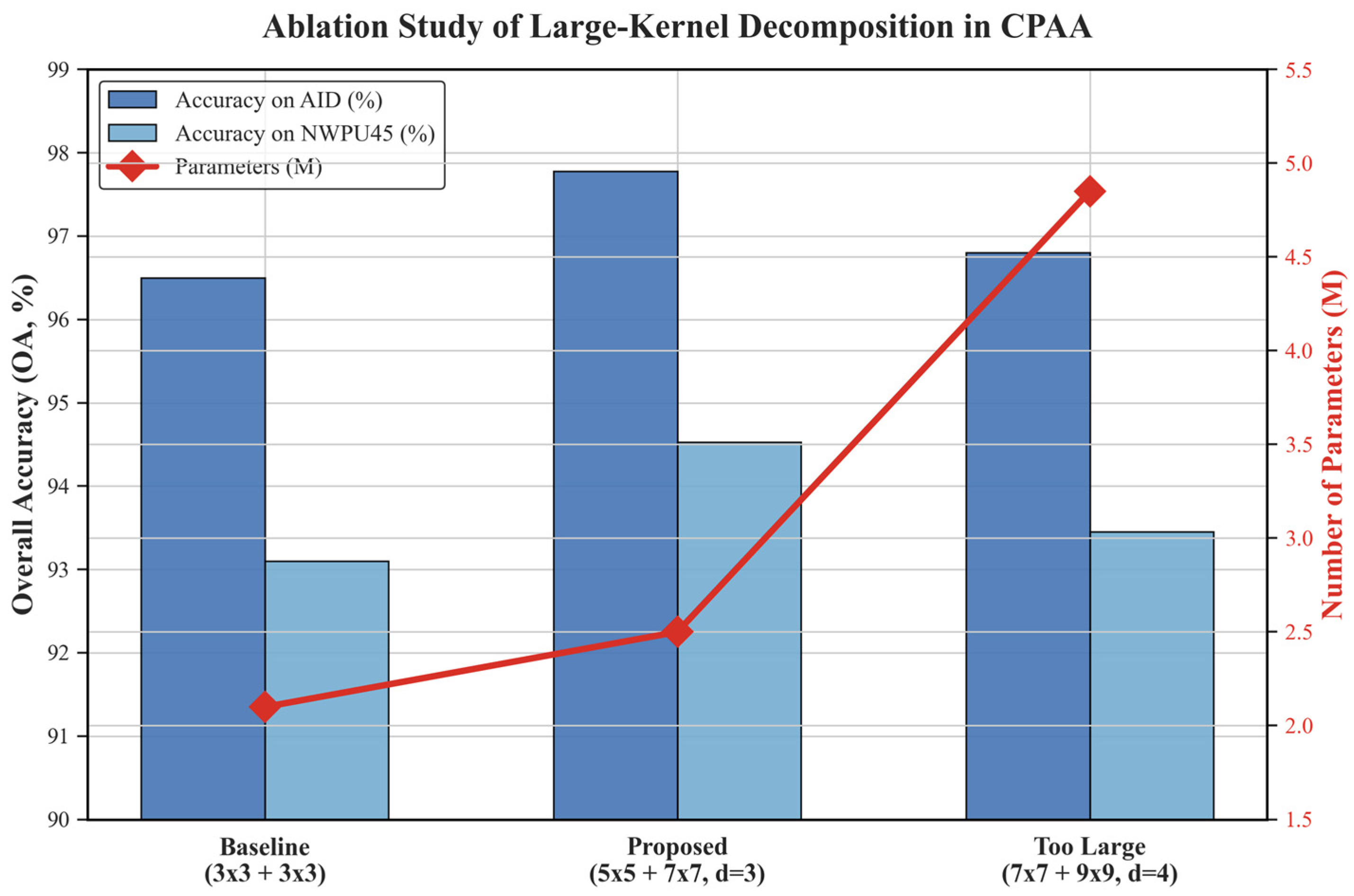
To delve deeper into the specific impacts of receptive field expansion strategies on model performance and spatial complexity, we evaluated three different convolutional kernel replacement schemes for the dilated convolutions in MDFE and the large-kernel decomposition in CPAA.
  • Standard Small Convs: Cancel all dilation mechanisms and large-sized convolutions in all modules. Replace all dilated convolutions (d = 2, 4) in the MDFE module and the 7 × 7 dilated convolutions in the CPAA module with standard 3 × 3 convolutions (d = 1).
  • Standard Large Convs: To achieve the same physical receptive field as our model without using dilation mechanisms, we forcibly enlarged the size of standard convolutional kernels. For instance, we replaced the 3 × 3 dilated convolution with d = 4 in MDFE with a 9 × 9 standard convolution, and the 7 × 7 dilated convolution with d = 3 in CPAA with a 19 × 19 standard convolution.
  • Proposed: Adopt the multi-dilation rate parallel MDFE architecture and the large-kernel decomposition strategy combining 5 × 5 and 7 × 7 dilated convolutions.
The experimental results are shown in Table 13. By comparison, we can draw the following conclusions:
  • Standard Small Convs Reduce Accuracy: When the network cancels all dilation mechanisms and relies solely on standard 3 × 3 convolutions, the parameter count drops slightly to 2.35 M, but the accuracy plummets. This proves that small receptive fields fail to establish effective long-range spatial dependencies in high-resolution scenes.
  • Standard Large Convs Increase Parameter Count: Attempting to obtain an equivalent receptive field by physically enlarging the standard convolutional kernels (such as 9 × 9 or 19 × 19) recovers some accuracy but causes the parameter count to surge to 14.72 M. Excessive parameters easily introduce redundant noise and hinder lightweight deployment.
  • Our Strategy Effectively Balances Parameters and Accuracy: Our scheme, utilizing a combination of multi-dilation rates and large-kernel decomposition, simulates an extremely large physical receptive field with only 2.50 M parameters. It achieves the highest accuracy across all three datasets, confirming that MS-DARNet maintains an excellent balance between large-scale environmental perception and model efficiency.

4.5.5. Sensitivity Analysis of Dilation Rates

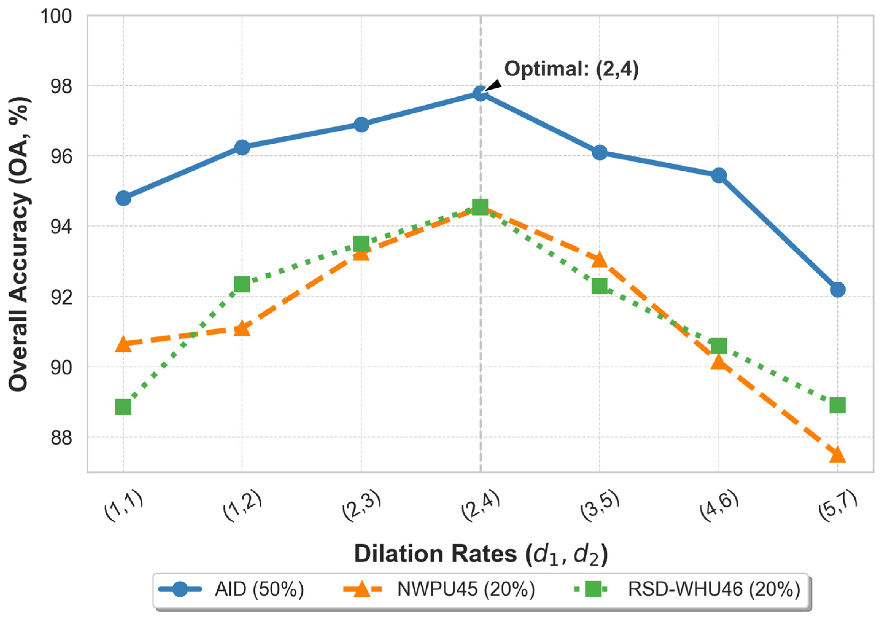
To investigate the impact of different receptive field expansion scales on feature extraction and to verify the cross-dataset stability of our hyperparameter choices, we conducted a systematic sensitivity analysis on the combination of dilation rates ( d ) in the parallel branches of the MDFE module. We expanded the test range from standard convolutions d = 1 , 1 to extreme dilation rates d = 5 , 7 , evaluating them comprehensively across the AID, NWPU45, and RSD-WHU46 datasets. The performance trends are illustrated in Figure 16.
As observed in Figure 16, the classification accuracy across all three datasets exhibits a highly consistent inverted V-shaped trend as the dilation rates increase.
  • Insufficient Receptive Field: When d = (1, 1), the module degrades to standard convolutions. Due to an insufficient receptive field, it fails to capture the global geometric structure of large-scale targets, yielding the lowest accuracy on all datasets. While combinations like d = (1, 2) and d = (2, 3) gradually improve performance, their spatial coverage remains limited for complex scenes.
  • The “Gridding Effect”: Conversely, excessively large dilation rates, such as d = (4, 6) and d = (5, 7), cause a sharp and continuous drop in accuracy. This decline occurs because overly sparse sampling intervals induce a severe “gridding effect,” causing the network to lose continuous local fine-grained textures (such as dense vehicles or distinct building edges). This is particularly detrimental in datasets with dense layouts like RSD-WHU46, where fine texture preservation is crucial for distinguishing similar scene categories.
  • Optimal Configuration: The proposed combination of d = (2, 4) consistently achieves the peak accuracy across all datasets (97.78% on AID, 94.53% on NWPU45, and 94.55% on RSD-WHU46). This uniform cross-dataset performance provides strong evidence that the d = (2, 4) configuration is not an empirical coincidence, but a generalized optimal scale that perfectly aligns with the statistical distribution of target sizes in high-resolution remote sensing scenes, effectively balancing local detail retention and broad contextual perception.

4.5.6. Effectiveness of Label Smoothing on Long-Tailed Distribution

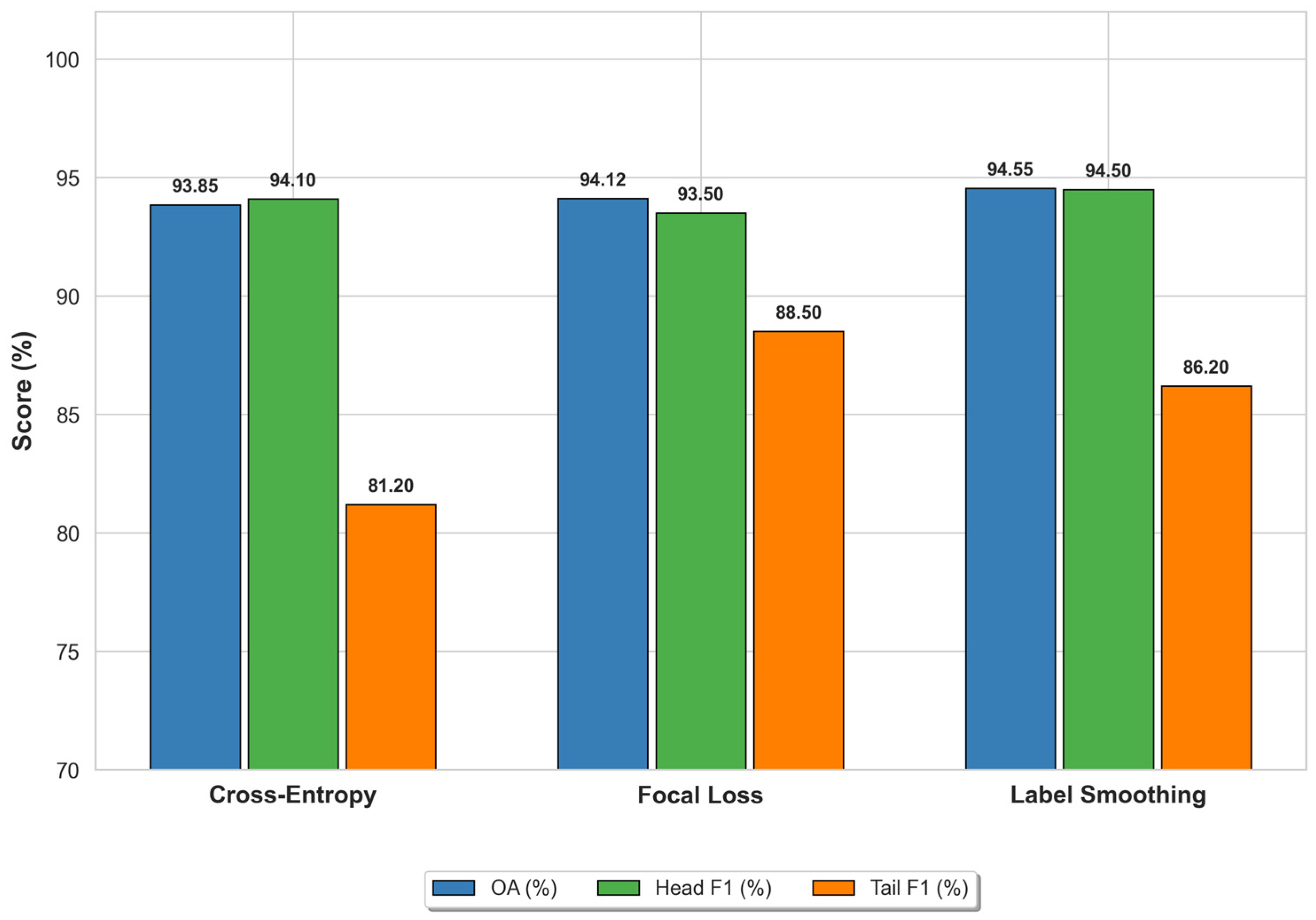
The RSD-WHU46 dataset exhibits a typical long-tailed distribution, containing head classes with abundant samples and tail classes with relatively limited samples. To evaluate the effectiveness of the LS strategy for addressing class imbalance, we compared it against the standard CE loss and Focal Loss on the RSD-WHU46 dataset with a 20% training ratio. The performance metrics, including Overall Accuracy (OA) and the F1-scores for representative head and tail classes, are illustrated in Figure 17.
As illustrated in Figure 17, the standard CE loss, which relies on “hard” targets, may render the network prone to overconfidence in head classes while potentially underrepresenting minority samples. This is reflected in a relatively lower tail class F1 score (81.20%). Focal Loss addresses this issue by allocating more gradient focus to harder-to-classify tail samples, yielding an improved tail class F1 score (88.50%). However, this resource reallocation appears to slightly compromise the feature learning of well-represented head classes, where the Head F1 score decreased to 93.50%.
In contrast, the Label Smoothing strategy ( ϵ = 0.1 ) achieved a favorable Overall Accuracy (94.55%) across the dataset. By introducing uniform soft targets, LS assists in mitigating the model’s tendency to form overconfident decision boundaries biased toward head classes. This approach contributes to an improved tail class performance (86.20%) while maintaining a competitive head class accuracy (94.50%). Although Focal Loss shows a marginal advantage on certain extreme tail categories, LS obviates the need for complex hyperparameter tuning (such as empirical selection of α and γ ). Consequently, it offers a generalized and stable optimization scheme, which aligns well with the efficient and practical design philosophy of the proposed lightweight model.

4.5.7. Effectiveness of the Mixed Activation Strategy

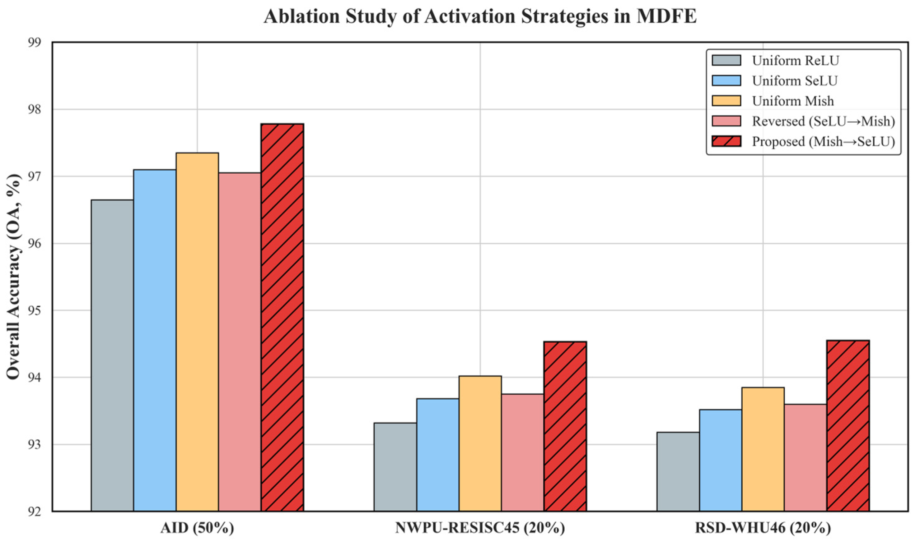
In the Multi-branch Dilated Feature Extraction (MDFE) module, we designed a specific mixed activation strategy: employing Mish in the initial feature extraction stage and switching to SeLU after the intermediate feature fusion. To provide rigorous mechanistic validation for this design choice, we conducted a comparative ablation study against uniform activation schemes (such as all-ReLU, all-Mish) and a reversed mixed scheme (SeLU Mish). The performance trajectories across the three datasets are visualized in Figure 18.
As illustrated in Figure 18, the traditional uniform ReLU setup yields the lowest accuracy across all datasets. This is attributed to the potential “dying ReLU” problem, which hard-truncates negative gradients and hinders the flow of subtle texture features in complex remote sensing scenes. While the uniform Mish (Mish Mish) setup improves gradient propagation due to its smooth, non-monotonic properties, its performance still plateaus. The underlying mechanism is that after the multi-branch features with different receptive fields are concatenated, the feature variance expands significantly. Continuing to use Mish fails to effectively constrain this variance shift.
Conversely, our proposed mixed strategy (Mish SeLU, highlighted in red hatched bars) consistently achieves the highest performance (97.78% on AID, 94.53% on NWPU45, and 94.55% on RSD-WHU46). Mish ensures maximal preservation of fine-grained spatial details during the initial decoupled extraction phase, while SeLU, with its inherent self-normalizing property, stabilizes the feature distribution variance immediately after the multi-scale fusion. The noticeably inferior performance of the reversed scheme (SeLU Mish) further mathematically corroborates that this specific sequence—“guiding gradient flow first, stabilizing distribution later”—is not an empirical coincidence but a structural necessity for robust multi-scale feature aggregation.

4.5.8. Validation of the Large-Kernel Decomposition Strategy in CPAA

To justify the specific kernel size selection ( 5 × 5 and 7 × 7 ,   d = 3 ) in the Selective Context Aggregation Branch (SCAB) of the CPAA module, we evaluated the trade-off between classification accuracy and parameter complexity under different kernel combinations. The results are presented as a dual-axis chart in Figure 19.
As shown by the blue and light-blue bars in Figure 19, the baseline configuration ( 3 × 3 + 3 × 3 ) requires minimal parameters (2.10 M) but delivers suboptimal accuracy. This confirms that small receptive fields fail to encompass the necessary macroscopic background required to suppress complex noise. On the other extreme, blindly expanding the kernels to a “Too Large” configuration ( 7 × 7 + 9 × 9 ,   d = 4 ) results in a performance drop alongside a sharp surge in parameters (indicated by the red line peaking at 4.85 M). This performance degradation occurs because an excessively large receptive field overly smooths the feature maps, inadvertently filtering out the ontological features of the core targets along with the background.
The proposed bionic configuration ( 5 × 5 + 7 × 7 ,   d = 3 ) explicitly hits the optimal “sweet spot.” It effectively expands the spatial context to simulate peripheral vision without inducing severe grid artifacts or feature dilution, achieving the highest accuracy while maintaining a highly compact footprint of only 2.50 M parameters. This solidifies the rationale behind our selective decomposition design over arbitrary kernel scaling.

4.5.9. Sensitivity Analysis of Minor Hyperparameters and Structural Choices

To fully address the sensitivity of the model to other specific structural choices, we evaluated the number of branches in the MDFE module, the ϵ value in label smoothing, and the placement of the BN layer in the STEM module. The results on the AID are summarized in Table 14.
  • Number of MDFE Branches: While increasing the number of parallel dilated branches from two (d = 2,4) to three (d = 2,4,6) yields a marginal accuracy improvement of 0.02%, it causes the parameter count to surge by 30% (from 2.50 M to 3.25 M). Therefore, the dual-branch setup is the optimal configuration for balancing computational efficiency and scale perception.
  • Label Smoothing ϵ Value: We tested ϵ values of 0.05, 0.10, and 0.20. Setting ϵ = 0.10 achieves the best overall accuracy. A smaller value (ϵ = 0.05) fails to sufficiently soften the boundaries for highly confused categories, while a larger value (ϵ = 0.20) introduces excessive uniform noise, disrupting the learning of distinct features.
  • Contribution of BN-before-Conv: We compared the standard post-activation sequence (Conv → BN → Mish) with our pre-activation sequence (BN → Conv → Mish). Our design improves accuracy by 0.43%. Normalizing the input distribution before the convolution effectively mitigates internal covariate shift at the very beginning of the network, ensuring a smoother gradient flow for subsequent high-resolution texture extraction.

5. Discussion

5.1. Advantages of Our Model

The MS-DARNet proposed in this paper exhibits outstanding classification performance across three highly challenging high-resolution remote sensing scene datasets (AID, NWPU-RESISC45, and RSD-WHU46), successfully striking an excellent balance between model lightweighting and high precision. This significant performance improvement is mainly attributed to the two core modules designed specifically for the challenges in remote sensing images. Addressing the significant scale variations in target objects in remote sensing scenes, traditional fixed-size convolutional kernels struggle to balance local details and global structures at the same feature level. The MDFE module in this paper introduces a dual-branch parallel dilated convolution architecture resembling a camera’s “zoom lens”. By combining convolution branches with dilation rates of 2 and 4, it dynamically expands the effective receptive field without increasing additional parameters (only 2.50 M). This enables the network to adaptively extract discriminative features of cross-scale targets, thereby excelling in complex scenes requiring macroscopic context support, such as “airports” or “commercial areas”. Addressing the extremely complex background noise and spatial layout challenges of dense objects in HRRSIs, the CPAA module proposed in this paper effectively overcomes the defects of traditional attention mechanisms and GAP. The SCAB within this module adopts a bionic large-kernel decomposition strategy (a 5 × 5 convolution combined with a 7 × 7 convolution with a dilation rate of 3) to explicitly decouple the ontological features of targets from the long-range global context. This enables the model to naturally filter out irrelevant background interference like the human visual system, performing excellently on artificial scene categories highly susceptible to environmental interference, such as “churches” and “palaces”. Concurrently, the PLAB branch aggregates features along horizontal and vertical directions to generate direction-aware vectors, re-embedding absolute position coordinate information and endowing the model with robust spatial structure parsing capabilities for densely arranged scenes such as “parking lots”. Furthermore, the introduction of the label smoothing regularization strategy effectively softens decision boundaries, substantially enhancing the model’s generalization robustness when confronting long-tail distribution datasets such as RSD-WHU46.

5.2. Limitations of the Model

5.2.1. General Limitations in Extreme Scenarios

Although MS-DARNet has achieved certain success, it still exposes some limitations when dealing with specific extreme visual conditions. Through an in-depth analysis of the confusion matrix, it can be discovered that when the model faces natural ground objects lacking distinct geometric structures and possessing highly similar underlying textures, the robustness of feature extraction is compromised. For instance, in the AID, 6% of “desert” samples were misclassified as “bare land”. This is primarily because these two types of scenes lack regular geometric structures, making it difficult for the PLAB branch to extract effective directional coordinate information.
Secondly, when confronting artificial scenes with similar macroscopic contextual environments and minimal core differences, the broad environmental perception capability of the SCAB is difficult to serve as an effective discriminative basis for distinguishing the two. For example, in the NWPU-RESISC45 dataset, there is a 9% inter-class confusion between “railway” and “railway station”. If the core structures (such as platforms) are too small in scale or lack salient features, the model struggles to achieve precise classification based solely on faint ontological features.
Finally, although the label smoothing mechanism effectively mitigates overconfidence and overfitting problems caused by class imbalance, it also causes the decision boundaries to become less sharp when the model learns categories with monotonous textures and blurred semantic boundaries. The 13% confusion rate between “square” and “dock” in the RSD-WHU46 dataset reflects the inadequacy of this strategy when processing highly homogenized categories.

5.2.2. Systematic Diagnostic Analysis of Failure Cases

To thoroughly comprehend the boundary conditions of MS-DARNet’s feature extraction capabilities, we conducted a systematic diagnostic analysis on the most challenging misclassified samples. We evaluated these failure cases through multi-dimensional visual and quantitative comparisons against the baseline network (ResNet-50).
  • Inter-class Similarity Visualization: As illustrated in Figure 20, the fundamental difficulty in distinguishing these specific category pairs stems from their extreme inter-class visual similarity across different dimensional attributes. In the AID, Desert and BareLand lack regular geometric structures, sharing almost identical homogeneous sandy textures and yellowish spectral responses. In the NWPU-RESISC45 dataset, Railway and Railway Station share the exact same macroscopic background—stretching parallel tracks and industrial contexts. Similarly, in the RSD-WHU46 dataset, both Square and Dock manifest as large expanses of flat, paved concrete. The absence of definitive semantic demarcations (such as explicit platforms for stations, or clear water-land boundaries for docks) in these orthophoto imageries establishes the primary hurdle for accurate scene parsing.
2.
Mechanism Diagnostic via Grad-CAM: To dissect how the networks process these ambiguous scenes, Figure 21 provides a comprehensive side-by-side diagnostic comparison. The baseline ResNet-50 uniformly struggles across all three scenarios: it exhibits scattered, uninformative blobs in the Desert, fragmented and loosely aligned focus in the Railway, and a massive diffuse activation in the Square. This indicates a failure to establish coherent spatial dependencies. In contrast, the proposed MS-DARNet generates structured and spatially specific activation patterns, reflecting the specific functioning of the CPAA module. Specifically, in the Desert scene, the attention is concentrated into a single focal point rather than being randomly dispersed. In the Railway scene, MS-DARNet activates along multiple parallel tracks, forming longitudinal geometric lines. In the Square scene, the network outlines a ‘T’-shaped geometric axis of the central pavement. However, these diagnostic maps also explicitly reveal the root cause of the model’s misclassifications: because the scenes lack their true class-specific architectural anchors, the model’s structural layout extraction forces it to over-fit onto these shared, non-discriminative local geometries (such as pure tracks or concrete axes), ultimately leading to biased predictions in highly homogenized scenarios.
3.
Feature Space Embedding Overlap: The algorithmic struggles observed in the attention maps are directly corroborated by the deep feature space distributions. As demonstrated by the t-SNE visualizations in Figure 22, severe feature entanglement is evident across all three datasets. For the Desert vs. BareLand pair, the feature embeddings show almost complete intermixing due to purely textural similarities. For the Railway vs. Station and Square vs. Dock pairs, while the network attempts to separate them based on extracted geometries, the massive overlap at the decision boundaries proves that the intra-class variance approaches the inter-class variance when critical semantic anchors are missing.
In summary, this comprehensive diagnostic analysis demonstrates that while MS-DARNet reduces the attention dispersion observed in standard CNNs by extracting prominent spatial layouts, its reliance on spatial geometric anchors limits its performance in purely texture-driven or boundary-ambiguous scenarios. This insight provides a clear trajectory for future work, emphasizing the necessity of integrating multi-modal data or specific fine-grained texture decoupling branches to further augment discriminative robustness.

5.3. Future Work Prospects

Addressing the aforementioned limitations, future research will primarily focus on the following directions to further refine the model. First, to improve the model’s classification performance on natural ground objects with no distinct boundaries and extremely high similarity (such as deserts and bare lands), we will explore more robust fine-grained feature mining mechanisms. For instance, integrating frequency-domain analysis to capture subtle textural variations, or employing unsupervised contrastive learning to enhance the representation of boundary-less features, could effectively reduce the network’s over-reliance on explicit geometric boundaries. Second, for highly similar scenes with highly consistent background environments, we will dedicate efforts to improving the fine-grained decoupling strategy at the feature level, further strengthening the model’s ability to capture core minute differences. Finally, regarding the classification difficulty of feature-monotonous scenes under long-tail distributions, future work needs to design more intelligent and adaptive boundary reinforcement strategies. Such strategies should not only effectively mitigate prediction biases brought by extreme class imbalances but also maintain the sharpness of decision boundaries in feature-scarce areas, thereby comprehensively enhancing the model’s discriminative and generalization capabilities in extremely complex remote sensing scenes.

6. Conclusions

Aiming at the severe challenges universally present in RSSC, including significant scale variations in target objects, strong interference from complex backgrounds, and the difficulty for existing models to achieve an ideal balance between computational performance and classification accuracy, this paper proposes MS-DARNet. The core advantage of this research lies in achieving efficient parsing of complex remote sensing scenes with low model complexity through an innovative pure convolutional architecture design. Specifically, this paper constructs the MDFE module, which ingeniously simulates the “macro” and “wide-angle” dual-lens mechanism of camera imaging. By fusing convolutional features with different dilation rates in parallel, it dynamically expands the effective receptive field without increasing the number of network parameters, effectively overcoming the limitation of traditional fixed-size convolutional kernels that struggle to balance global geometric structures and fine-grained local textures simultaneously. Simultaneously, to further enhance feature discriminability and suppress noise, this paper designs the CPAA module. The SCAB within this module adopts a bionic large-kernel decomposition strategy, capable of precisely filtering redundant background interference while perceiving broad environmental contexts. Meanwhile, PLAB discards the GAP operation and re-embeds crucial two-dimensional spatial coordinate information into the feature map through a direction-aware vector reconstruction technique, endowing the model with an exceptionally strong spatial structure parsing capability for densely arranged scenes.
Furthermore, combined with the label smoothing regularization strategy, our model effectively enhances generalization robustness when dealing with long-tail distributions and highly similar, easily confusable categories, mitigating the overfitting problem caused by overconfidence. Comprehensive experiments on three challenging large-scale public datasets, including AID, NWPU-RESISC45, and RSD-WHU46, demonstrate that MS-DARNet exhibits outstanding classification performance, achieving overall accuracies of 97.78%, 94.53%, and 94.55%, respectively. Compared to existing mainstream classic networks and advanced lightweight models, MS-DARNet achieves an optimal balance between classification accuracy and computational efficiency with a parameter count of merely 2.50 M and a computational cost of 0.5940 GMACs, fully proving its immense potential for practical deployment on resource-constrained Earth observation equipment, such as onboard real-time classification for small satellites or unmanned aerial systems (UAS). To adapt MS-DARNet for these specific edge-computing scenarios in practice, practitioners would primarily need to perform post-training quantization (such as converting FP32 weights to INT8 or FP16 formats) to further compress the memory footprint and reduce energy consumption. Additionally, exporting the PyTorch-trained model to hardware-accelerated inference engines, such as TensorRT or ONNX Runtime, would be a necessary engineering step to fully exploit the parallel computing capabilities of embedded GPUs (such as NVIDIA Jetson series) or dedicated Neural Processing Units (NPUs). These standard adaptation steps will bridge the gap between our theoretical lightweight design and physical hardware deployment. However, through in-depth analysis of the confusion matrix, it was also discovered that the model still suffers from insufficient fine-grained feature decoupling when processing certain homogenized natural ground objects lacking distinct geometric boundaries and possessing extremely similar underlying textures (such as “desert” and “bare land”) or artificial flat areas (such as “square” and “dock”). Future research will be dedicated to exploring more adaptive boundary reinforcement strategies and subtle feature mining mechanisms to further improve the model’s discriminative robustness in extremely confusing scenes.
Our code is publicly available at https://github.com/Chengjunxu-whu/vfcrecognition (accessed on 8 April 2026).

Author Contributions

Conceptualization, J.H. and C.X.; methodology, J.H.; software, J.H.; validation, J.H. and C.X.; formal analysis, J.H.; investigation, J.H.; data curation, J.H.; writing—original draft preparation, J.H.; writing—review and editing, C.X.; visualization, J.H.; supervision, C.X.; project administration, C.X.; funding acquisition, C.X. All authors have read and agreed to the published version of the manuscript.

Funding

This research was funded by the National Natural Science Foundation of China (42261068) and the Natural Science Foundation of Jiangxi Province (20242BAB25112).

Data Availability Statement

The data presented in this study are openly available in the Aerial Imagery Dataset (AID) at https://captain-whu.github.io/AID/ (accessed on 28 February 2026), NWPU-RESISC45 Dataset at https://gcheng-nwpu.github.io/#Datasets (accessed on 28 February 2026), and RSD-WHU46 Dataset at https://github.com/RSIA-LIESMARS-WHU/RSD46-WHU (accessed on 28 February 2026).

Acknowledgments

During the preparation of this manuscript, the authors used Gemini 3.0 for the purposes of English language editing and text refinement in the abstract and highlights. The authors have reviewed and edited the output and take full responsibility for the content of this publication.

Conflicts of Interest

The authors declare no conflicts of interest.

Abbreviations

The following abbreviations are used in this manuscript:
AIDAerial Imagery Dataset
BNBatch Normalization
BoVWBag-of-Visual-Words
CECross-Entropy
CNNConvolutional Neural Network
CPAAContext-Position Aware Attention
CPUCentral Processing Unit
DConvDilated Convolution
DMCCADiscriminative Multiple Canonical Correlation Analysis
DTCDifferentiable Token Compression
DWConvDepth-Wise Separable Convolution
ECAEfficient Channel Attention
GAPGlobal Average Pooling
GELUGaussian Error Linear Unit
GMACsGiga Multiply–Accumulate Operations
GPUGraphics Processing Unit
HOGHistogram of Oriented Gradients
HRRSIHigh-Resolution Remote Sensing Image
IRCHKDInverted Residual Cross Head Knowledge Distillation Network
LDALatent Dirichlet Allocation
LMHMambaLightweight Multifeature Hybrid Mamba
LSMNetLarge Kernel Separable Mixed Convolutional Network
MDFEMulti-branch Dilated Feature Extraction
MS-DARNetMulti-Scale Selective Dilated Attention Residual Network
OAOverall Accuracy
PLABPrecise Location-Aware Branch
RSD-WHU46Remote Sensing Dataset Wuhan University 46
ReLURectified Linear Unit
RSIRemote Sensing Image
RSSCRemote Sensing Scene Classification
SCABSelective Context Aggregation Branch
SDT2NetSecond-Order Differentiable Token Transformer Network
SeLUScaled Exponential Linear Unit
SGDStochastic Gradient Descent
SIFTScale-Invariant Feature Transform
SSMsState Space Models
STMSFSwin Transformer with Multi-Scale Fusion

References

  1. Cheng, G.; Xie, X.; Han, J.; Guo, L.; Xia, G.S. Remote sensing image scene classification meets deep learning: Challenges, methods, benchmarks, and opportunities. IEEE J. Sel. Top. Appl. Earth Obs. Remote Sens. 2020, 13, 3735–3756. [Google Scholar] [CrossRef]
  2. Li, D.; Wang, M.; Dong, Z.; Shen, X.; Shi, L. Earth observation brain (EOB): An intelligent earth observation system. Geo-Spat. Inf. Sci. 2017, 20, 134–140. [Google Scholar] [CrossRef]
  3. Xu, C.; Zhu, G.; Shu, J. Lie Group Spatial Attention Mechanism Model for Remote Sensing Scene Classification. Int. J. Remote Sens. 2022, 43, 2461–2474. [Google Scholar] [CrossRef]
  4. Xu, C.; Shu, J.; Zhu, G. Multi-Feature Dynamic Fusion Cross-Domain Scene Classification Model Based on Lie Group Space. Remote Sens. 2023, 15, 4790. [Google Scholar] [CrossRef]
  5. Martha, T.R.; Kerle, N.; Van Westen, C.J.; Jetten, V.; Kumar, K.V. Segment Optimization and Data-Driven Thresholding for Knowledge-Based Landslide Detection by Object-Based Image Analysis. IEEE Trans. Geosci. Remote Sens. 2011, 49, 4928–4943. [Google Scholar] [CrossRef]
  6. Li, J.; Hong, D.; Gao, L.; Yao, J.; Zheng, K.; Zhang, B.; Chanussot, J. Deep Learning in Multimodal Remote Sensing Data Fusion: A Comprehensive Review. Int. J. Appl. Earth Obs. Geoinf. 2022, 112, 102926. [Google Scholar] [CrossRef]
  7. Artime, O.; Grassia, M.; De Domenico, M.; Gleeson, J.P.; Makse, H.A.; Mangioni, G.; Perc, M.; Radicchi, F. Robustness and resilience of complex networks. Nat. Rev. Phys. 2024, 6, 114–131. [Google Scholar] [CrossRef]
  8. Ji, J.; Zhao, Y.; Li, A.; Ma, X.; Wang, C.; Lin, Z. Dense small object detection algorithm for unmanned aerial vehicle remote sensing images in complex backgrounds. Digit. Signal Process. 2025, 158, 104938. [Google Scholar] [CrossRef]
  9. Xia, G.S.; Hu, J.; Hu, F.; Shi, B.; Bai, X.; Zhong, Y.; Zhang, L.; Lu, X. AID: A benchmark dataset for performance evaluation of aerial scene classification. IEEE Trans. Geosci. Remote Sens. 2017, 55, 3965–3981. [Google Scholar] [CrossRef]
  10. Zhang, J.; Li, W.; Ogunbona, P. Joint Geometrical and Statistical Alignment for Visual Domain Adaptation. In Proceedings of the 2017 IEEE Conference on Computer Vision and Pattern Recognition (CVPR), Honolulu, HI, USA, 21–26 July 2017; IEEE: New York, NY, USA, 2017; pp. 5150–5158. [Google Scholar] [CrossRef]
  11. Yin, Z.; Wu, M.; Niu, Z.; Wang, L.; Dou, C. Streetlight density and quantity estimation using glimmer images from SDGSAT-1. Remote Sens. Environ. 2026, 333, 115119. [Google Scholar] [CrossRef]
  12. Lowe, D.G. Distinctive image features from scale-invariant keypoints. Int. J. Comput. Vis. 2004, 60, 91–110. [Google Scholar] [CrossRef]
  13. Dalal, N.; Triggs, B. Histograms of oriented gradients for human detection. In Proceedings of the 2005 IEEE Computer Society Conference on Computer Vision and Pattern Recognition (CVPR’05), San Diego, CA, USA, 20–25 June 2005; IEEE: New York, NY, USA, 2005; pp. 886–893. [Google Scholar] [CrossRef]
  14. Yang, Y.; Newsam, S. Bag-of-visual-words and spatial extensions for land-use classification. In Proceedings of the 18th SIGSPATIAL International Conference on Advances in Geographic Information Systems, San Jose, CA, USA, 2–5 November 2010; pp. 270–279. [Google Scholar] [CrossRef]
  15. Li, Y.; Wu, Y.; Cheng, G.; Tao, C.; Dang, B.; Wang, Y.; Zhang, J.; Zhang, C.; Liu, Y.; Tang, X.; et al. MEET: A million-scale dataset for fine-grained geospatial scene classification with zoom-free remote sensing imagery. IEEE/CAA J. Autom. Sin. 2025, 12, 1004–1023. [Google Scholar] [CrossRef]
  16. Dong, H.; Li, J.; Ma, Z.; Li, Z.; Liu, M.; Wei, X.; Jiao, L. A lightweight multifeature hybrid Mamba for remote sensing image scene classification. IEEE Geosci. Remote Sens. Lett. 2026, 23, 6000705. [Google Scholar] [CrossRef]
  17. Li, F.; Wang, X.; Wang, H.; Karimian, H.; Shi, J.; Zha, G. LMVMamba: A hybrid U-shape Mamba for remote sensing segmentation with adaptation fine-tuning. Remote Sens. 2025, 17, 3367. [Google Scholar] [CrossRef]
  18. Gao, H.; Wu, S.; Wang, Y.; Kim, J.; Xu, Y. Fsod4rsi: Few-Shot Object Detection for Remote Sensing Images via Features Aggregation and Scale Attention. IEEE J. Sel. Top. Appl. Earth Obs. Remote Sens. 2024, 17, 4784–4796. [Google Scholar] [CrossRef]
  19. Zhou, H.; Liu, W.; Sun, K.; Wu, J.; Wu, T. MSCANet: A Multi-Scale Context-Aware Network for Remote Sensing Object Detection. Earth Sci. Inform. 2024, 17, 5521–5538. [Google Scholar] [CrossRef]
  20. Liu, Y.; Li, H.; Hu, C.; Luo, S.; Luo, Y.; Chen, C.W. Learning to Aggregate Multi-Scale Context for Instance Segmentation in Remote Sensing Images. IEEE Trans. Neural Netw. Learn. Syst. 2024, 36, 595–609. [Google Scholar] [CrossRef]
  21. Shi, C.; Ding, M.; Wang, L. Reparameterized Feature Aggregation Convolutional Neural Network for Remote Sensing Scene Image Classification. IEEE J. Sel. Top. Appl. Earth Obs. Remote Sens. 2025, 18, 12603–12615. [Google Scholar] [CrossRef]
  22. Xu, C.; Shu, J.; Wang, Z.; Wang, J. A Scene Classification Model Based on Global-Local Features and Attention in Lie Group Space. Remote Sens. 2024, 16, 2323. [Google Scholar] [CrossRef]
  23. Ma, X.; Luo, J.; Ni, S.; Zhang, X.; Ding, R. SDLS: A Two-Stream Architecture with Self-Distillation and Local Streams for Remote Sensing Image Scene Classification. Remote Sens. 2026, 18, 498. [Google Scholar] [CrossRef]
  24. Sukul, A.R.; Jamali, A.; Roy, S.K.; Bhattacharya, A.; Ghamisi, P. Cross hyperspectral and LiDAR attention transformer: An extended self-attention for land use and land cover classification. IEEE Trans. Geosci. Remote Sens. 2024, 62, 5512815. [Google Scholar] [CrossRef]
  25. Wang, Y.; Tai, M.; Liu, Z.; Shu, Z.; Xiong, F.; Yu, Z. Mid-range convolutional modulated transformer network for hyperspectral image classification. IEEE Trans. Geosci. Remote Sens. 2025, 63, 5532315. [Google Scholar] [CrossRef]
  26. Lu, W.; Nguyen, M. Dual sparsity transformer with contour loss for real-time UAV semantic segmentation. IEEE Trans. Geosci. Remote Sens. 2025, 63, 4416816. [Google Scholar] [CrossRef]
  27. Fang, X.; Liu, Z.; Xie, S.; Ge, Y. Semantic segmentation of high-resolution remote sensing images based on RS3Mamba. Remote Sens. 2025, 17, 3443. [Google Scholar] [CrossRef]
  28. Hong, D.; Zhang, B.; Li, X.; Li, Y.; Li, C.; Yao, J.; Yokoya, N.; Li, H.; Ghamisi, P.; Jia, X.; et al. SpectralGPT: Spectral Remote Sensing Foundation Model. IEEE Trans. Geosci. Remote Sens. 2024, 46, 5227–5244. [Google Scholar] [CrossRef] [PubMed]
  29. Li, R.; Cao, C. Remote sensing image scene classification based on ResNet-18 and attention mechanism. In Proceedings of the International Conference on Optoelectronics, Computer Science, and Algorithms (OCSA 2025), Changsha, China, 19–21 September 2025; SPIE: Bellingham, WA, USA, 2026; Volume 14008, p. 140080E. [Google Scholar] [CrossRef]
  30. Wang, R.; Ma, L.; He, G.; Johnson, B.A.; Yan, Z.; Chang, M.; Liang, Y. Transformers for Remote Sensing: A Systematic Review and Analysis. Sensors 2024, 24, 3495. [Google Scholar] [CrossRef]
  31. Chen, H.; Song, J.; Han, C.; Xia, J.; Yokoya, N. ChangeMamba: Remote Sensing Change Detection With Spatiotemporal State Space Model. IEEE Trans. Geosci. Remote Sens. 2024, 62, 4409720. [Google Scholar] [CrossRef]
  32. He, X.; Cao, K.; Zhang, J.; Yan, K.; Wang, Y.; Li, R.; Xie, C.; Hong, D.; Zhou, M. PanMamba: Effective Pan-Sharpening With State Space Model. Inf. Fusion 2024, 115, 102779. [Google Scholar] [CrossRef]
  33. Zhu, Q.; Cai, Y.; Fang, Y.; Yang, Y.; Chen, C.; Fan, L.; Nguyen, A. Samba: Semantic Segmentation of Remotely Sensed Images With State Space Model. Heliyon 2024, 10, e38495. [Google Scholar] [CrossRef]
  34. Ma, X.; Zhang, X.; Pun, M.O. RS3Mamba: Visual State Space Model for Remote Sensing Image Semantic Segmentation. IEEE Geosci. Remote Sens. Lett. 2024, 21, 6011405. [Google Scholar] [CrossRef]
  35. Yao, J.; Hong, D.; Li, C.; Chanussot, J. SpectralMamba: Efficient Mamba for Hyperspectral Image Classification. arXiv 2024, arXiv:2404.08489. [Google Scholar] [CrossRef]
  36. Li, Y.; Li, D.; Xie, W.; Ma, J.; He, S.; Fang, L. Semi-Mamba: Mamba-Driven Semi-Supervised Multimodal Remote Sensing Feature Classification. IEEE Trans. Circuits Syst. Video Technol. 2025, 35, 9837–9849. [Google Scholar] [CrossRef]
  37. Yan, L.; Zhang, X.; Wang, K.; Zhang, D. Contour-Enhanced Visual State-Space Model for Remote Sensing Image Classification. IEEE Trans. Geosci. Remote Sens. 2025, 63, 5603614. [Google Scholar] [CrossRef]
  38. Li, D.; Liu, R.; Liu, Y. MPFASS-Net: A Mamba Progressive Feature Aggregation Network With Self-Supervised for Remote Sensing Image Scene Classification. IEEE Trans. Geosci. Remote Sens. 2025, 63, 5523614. [Google Scholar] [CrossRef]
  39. Blei, D.M.; Ng, A.Y.; Jordan, M.I. Latent dirichlet allocation. J. Mach. Learn. Res. 2003, 3, 993–1022. [Google Scholar]
  40. Zhang, K.; Cui, T.; Wu, W.; Zheng, X.; Cheng, G. Large Kernel Separable Mixed ConvNet for Remote Sensing Scene Classification. IEEE J. Sel. Top. Appl. Earth Obs. Remote Sens. 2024, 17, 4294–4303. [Google Scholar] [CrossRef]
  41. Wang, G.; Wen, X.; Xu, H.; Wang, X. LFNet: A Frequency–Texture Fusion Network With Distance Correlation Loss for Remote Sensing Scene Classification. IEEE J. Sel. Top. Appl. Earth Obs. Remote Sens. 2026, 19, 6809–6826. [Google Scholar] [CrossRef]
  42. Shi, C.; Ding, M.; Wang, L. An Inverted Residual Cross Head Knowledge Distillation Network for Remote Sensing Scene Image Classification. IEEE J. Sel. Top. Appl. Earth Obs. Remote Sens. 2025, 18, 4881–4894. [Google Scholar] [CrossRef]
  43. Fazilov, S.; Yusupov, O.; Khandamov, Y.; Eshonqulov, E.; Khamidov, J.; Abdieva, K. Remote Sensing Scene Classification via Multi-Feature Fusion Based on Discriminative Multiple Canonical Correlation Analysis. AI 2026, 7, 5. [Google Scholar] [CrossRef]
  44. Duan, Y.; Song, C.; Zhang, Y.; Cheng, P.; Mei, S. STMSF: Swin Transformer with Multi-Scale Fusion for Remote Sensing Scene Classification. Remote Sens. 2025, 17, 668. [Google Scholar] [CrossRef]
  45. Ni, K.; Wu, Q.; Li, S.; Zheng, Z.; Wang, P. Remote Sensing Scene Classification via Second-Order Differentiable Token Transformer Network. IEEE Trans. Geosci. Remote Sens. 2026, 62, 5626915. [Google Scholar] [CrossRef]
  46. Chen, K.; Chen, B.; Liu, C.; Li, W.; Zou, Z.; Shi, Z. RSMamba: Remote Sensing Image Classification with State Space Model. IEEE Geosci. Remote Sens. Lett. 2024, 21, 8002605. [Google Scholar] [CrossRef]
  47. Wang, G.; Zhang, X.; Peng, Z.; Zhang, T.; Jiao, L. S2Mamba: A Spatial-Spectral State Space Model for Hyperspectral Image Classification. IEEE Trans. Geosci. Remote Sens. 2025, 63, 5511413. [Google Scholar] [CrossRef]
  48. Xu, C.; Zhu, G.; Shu, J. A Combination of Lie Group Machine Learning and Deep Learning for Remote Sensing Scene Classification Using Multi-Layer Heterogeneous Feature Extraction and Fusion. Remote Sens. 2022, 14, 1445. [Google Scholar] [CrossRef]
  49. Zhang, Z.; Xu, C. A Lie Group-Based Model for Remote Scene Classification With Multi-Scale Feature Fusion and Mixed Attention Mechanisms. Int. J. Remote Sens. 2025, 46, 3800–3830. [Google Scholar] [CrossRef]
  50. Xu, C.; Shu, J.; Wang, Z.; Wang, J. Dynamic Convolutional Model Based on Distribution-Collaboration Strategy for Remote Sensing Scene Classification. Int. J. Digit. Earth 2025, 18, 2517824. [Google Scholar] [CrossRef]
  51. Yang, C.; Wei, C.; Zhao, Y.; Wang, L.; Xu, P.; Qi, K.; Shao, Y.; Wu, H. MSALNet: A multi-scale adaptive learning network for high-resolution remote sensing scene classification. Geo-Spat. Inf. Sci. 2025, 29, 143–167. [Google Scholar] [CrossRef]
  52. Dai, H.; Yue, Y.; Liu, Q. Hyperspectral Image Classification Based on Hybrid Depth-Wise Separable Convolution and Dual-Branch Feature Fusion Network. Appl. Sci. 2025, 15, 1394. [Google Scholar] [CrossRef]
  53. Chong, Y.; Ge, X.; Pan, S. RISNet: Robust Ill-Posed Solver for Remote Sensing Image Change Detection. IEEE J. Sel. Top. Appl. Earth Obs. Remote Sens. 2025, 18, 7625–7639. [Google Scholar] [CrossRef]
  54. Huang, F.; Guo, Y. Spatial structure-aware and cross-scale feature modeling network for remote sensing image semantic segmentation. Electron. Res. Arch. 2025, 33, 6391–6417. [Google Scholar] [CrossRef]
  55. Perdana, R.A.; Arimurthy, A.M.; Risnandar. Remote Sensing Scene Classification using ConvNeXt-Tiny Model with Attention Mechanism and Label Smoothing. J. RESTI (Rekayasa Sist. Teknol. Inf.) 2024, 8, 389–400. [Google Scholar] [CrossRef]
  56. Szegedy, C.; Vanhoucke, V.; Ioffe, S.; Shlens, J.; Wojna, Z. Rethinking the Inception Architecture for Computer Vision. In Proceedings of the 2016 IEEE Conference on Computer Vision and Pattern Recognition (CVPR), Las Vegas, NV, USA, 27–30 June 2016; IEEE: New York, NY, USA, 2016; pp. 2818–2826. [Google Scholar] [CrossRef]
  57. Long, Y.; Gong, Y.; Xiao, Z.; Liu, Q. Accurate object localization in remote sensing images based on convolutional neural networks. IEEE Trans. Geosci. Remote Sens. 2017, 55, 2486–2498. [Google Scholar] [CrossRef]
  58. Xiao, Z.; Long, Y.; Li, D.; Wei, C.; Tang, G.; Liu, J. High-Resolution Remote Sensing Image Retrieval Based on CNNs from a Dimensional Perspective. Remote Sens. 2017, 9, 725. [Google Scholar] [CrossRef]
  59. Paszke, A.; Gross, S.; Massa, F.; Lerer, A.; Bradbury, J.; Chanan, G.; Killeen, T.; Lin, Z.; Gimelshein, N.; Antiga, L.; et al. PyTorch: An imperative style, high-performance deep learning library. Adv. Neural Inf. Process. Syst. 2019, 32, 8024–8035. [Google Scholar] [CrossRef]
  60. Chaib, S.; Liu, H.; Gu, Y.; Yao, H. Deep Feature Fusion for VHR Remote Sensing Scene Classification. IEEE Trans. Geosci. Remote Sens. 2017, 55, 4775–4784. [Google Scholar] [CrossRef]
  61. Anwer, R.M.; Khan, F.S.; Van De Weijer, J.; Molinier, M.; Laaksonen, J. Binary Patterns Encoded Convolutional Neural Networks for Texture Recognition and Remote Sensing Scene Classification. ISPRS J. Photogramm. Remote Sens. 2018, 138, 74–85. [Google Scholar] [CrossRef]
  62. Bi, Q.; Qin, K.; Zhang, H.; Xie, J.; Li, Z.; Xu, K. APDC-Net: Attention Pooling-Based Convolutional Network for Aerial Scene Classification. IEEE Geosci. Remote Sens. Lett. 2019, 17, 1603–1607. [Google Scholar] [CrossRef]
  63. Li, W.; Wang, Z.; Wang, Y.; Wu, J.; Wang, J.; Jia, Y.; Gui, G. Classification of High-SpatialResolution Remote Sensing Scenes Method Using Transfer Learning and Deep Convolutional Neural Network. IEEE J. Sel. Top. Appl. Earth Obs. Remote Sens. 2020, 13, 1986–1995. [Google Scholar] [CrossRef]
  64. Wan, Q.; Xiao, Z.; Yu, Y.; Liu, Z.; Wang, K.; Li, D. A Hyperparameter-Free Attention Module Based on Feature Map Mathematical Calculation for Remote-Sensing Image Scene Classification. IEEE Trans. Geosci. Remote Sens. 2023, 62, 5600318. [Google Scholar] [CrossRef]
  65. Aral, R.A.; Keskin, ŞR.; Kaya, M.; Hacömeroğlu, M. Classification of Trashnet Dataset Based on Deep Learning Models. In Proceedings of the 2018 IEEE International Conference on Big Data (Big Data), Seattle, WA, USA, 10–13 December 2018; IEEE: New York, NY, USA, 2018; pp. 2058–2062. [Google Scholar]
  66. Lawrence, R.L.; Wood, S.D.; Sheley, R.L. Mapping Invasive Plants Using Hyperspectral Imagery and Breiman Cutler Classifications (RandomForest). Remote Sens. Environ. 2006, 100, 356–362. [Google Scholar] [CrossRef]
  67. Xu, C.; Zhu, G.; Shu, J. A Lightweight and Robust Lie Group-Convolutional Neural Networks Joint Representation for Remote Sensing Scene Classification. IEEE Trans. Geosci. Remote Sens. 2021, 60, 5501415. [Google Scholar] [CrossRef]
  68. Xu, X.; Xu, C. Towards Lightweight and Multi-Scale Scene Classification: A Lie Group-Guided Deep Learning Network with Collaborative Attention. J. Imaging 2026, 12, 94. [Google Scholar] [CrossRef] [PubMed]
  69. Lu, Y.; Sun, M. Lightweight multidimensional feature enhancement algorithm LPS-YOLO for UAV remote sensing target detection. Sci. Rep. 2025, 15, 1340. [Google Scholar] [CrossRef] [PubMed]
  70. Liang, J.; Deng, Y.; Zeng, D. A Deep Neural Network Combined CNN and GCN for Remote Sensing Scene Classification. IEEE J. Sel. Top. Appl. Earth Obs. Remote Sens. 2020, 13, 4325–4338. [Google Scholar] [CrossRef]
  71. Shi, C.; Zhang, X.; Wang, L. A Lightweight Convolutional Neural Network Based on Channel Multi-Group Fusion for Remote Sensing Scene Classification. Remote Sens. 2022, 14, 9. [Google Scholar] [CrossRef]
  72. Chollet, F. Xception: Deep Learning with Depthwise Separable Convolutions. In Proceedings of the 2017 IEEE Conference on Computer Vision and Pattern Recognition (CVPR), Honolulu, HI, USA, 21–26 July 2017; IEEE: New York, NY, USA, 2017; pp. 1251–1258. [Google Scholar] [CrossRef]
  73. Zhang, B.; Zhang, Y.; Wang, S. A Lightweight and Discriminative Model for Remote Sensing Scene Classification With Multidilation Pooling Module. IEEE J. Sel. Top. Appl. Earth Obs. Remote Sens. 2020, 12, 2636–2653. [Google Scholar] [CrossRef]
  74. Liu, G.; Kang, H.; Wang, Q.; Tian, Y.; Wan, B. Contourlet-CNN for SAR Image Despeckling. Remote Sens. 2021, 13, 764. [Google Scholar] [CrossRef]
  75. Shi, C.; Zhang, X.; Sun, J.; Wang, L. Remote Sensing Scene Image Classification Based on Self-Compensating Convolution Neural Network. Remote Sens. 2022, 14, 545. [Google Scholar] [CrossRef]
  76. Shi, C.; Zhang, X.; Sun, J.; Wang, L. A Lightweight Convolutional Neural Network Based on Group-Wise Hybrid Attention for Remote Sensing Scene Classification. Remote Sens. 2022, 14, 161. [Google Scholar] [CrossRef]
  77. Zhang, Z.; Liu, S.; Zhang, Y.; Chen, W. RS-DARTS: A Convolutional Neural Architecture Search for Remote Sensing Image Scene Classification. Remote Sens. 2022, 14, 141. [Google Scholar] [CrossRef]
  78. Krizhevsky, A.; Sutskever, I.; Hinton, G.E. ImageNet classification with deep convolutional neural networks. Commun. ACM 2017, 60, 84–90. [Google Scholar] [CrossRef]
  79. Hu, J.; Shen, L.; Sun, G. Squeeze-and-Excitation Networks. In Proceedings of the 2018 IEEE/CVF Conference on Computer Vision and Pattern Recognition, Salt Lake City, UT, USA, 18–23 June 2018; IEEE: New York, NY, USA, 2018; pp. 7132–7141. [Google Scholar] [CrossRef]
  80. Iandola, F.N.; Han, S.; Moskewicz, M.W.; Ashraf, K.; Dally, W.J.; Keutzer, K. SqueezeNet: AlexNet-level accuracy with 50x fewer parameters and <0.5MB model size. arXiv 2016, arXiv:1602.07360. [Google Scholar] [CrossRef]
  81. Ma, N.; Zhang, X.; Zheng, H.; Sun, J. ShuffleNet V2: Practical Guidelines for Efficient CNN Architecture Design. In Proceedings of the European Conference on Computer Vision (ECCV 2018), Munich, Germany, 8–14 September 2018; pp. 116–131. [Google Scholar] [CrossRef]
  82. Tan, M.; Le, Q. EfficientNet: Rethinking Model Scaling for Convolutional Neural Networks. In Proceedings of the 36th International Conference on Machine Learning, Long Beach, CA, USA, 9–15 June 2019; pp. 6105–6114. [Google Scholar]
  83. Zhang, T.; Wang, Z.; Cheng, P.; Xu, G.; Sun, X. DCNNet: A Distributed Convolutional Neural Network for Remote Sensing Image Scene Classification. IEEE Trans. Geosci. Remote Sens. 2023, 61, 5603618. [Google Scholar] [CrossRef]
  84. Simonyan, K.; Zisserman, A. Very Deep Convolutional Networks for Large-Scale Image Recognition. arXiv 2014, arXiv:1409.1556. [Google Scholar] [CrossRef]
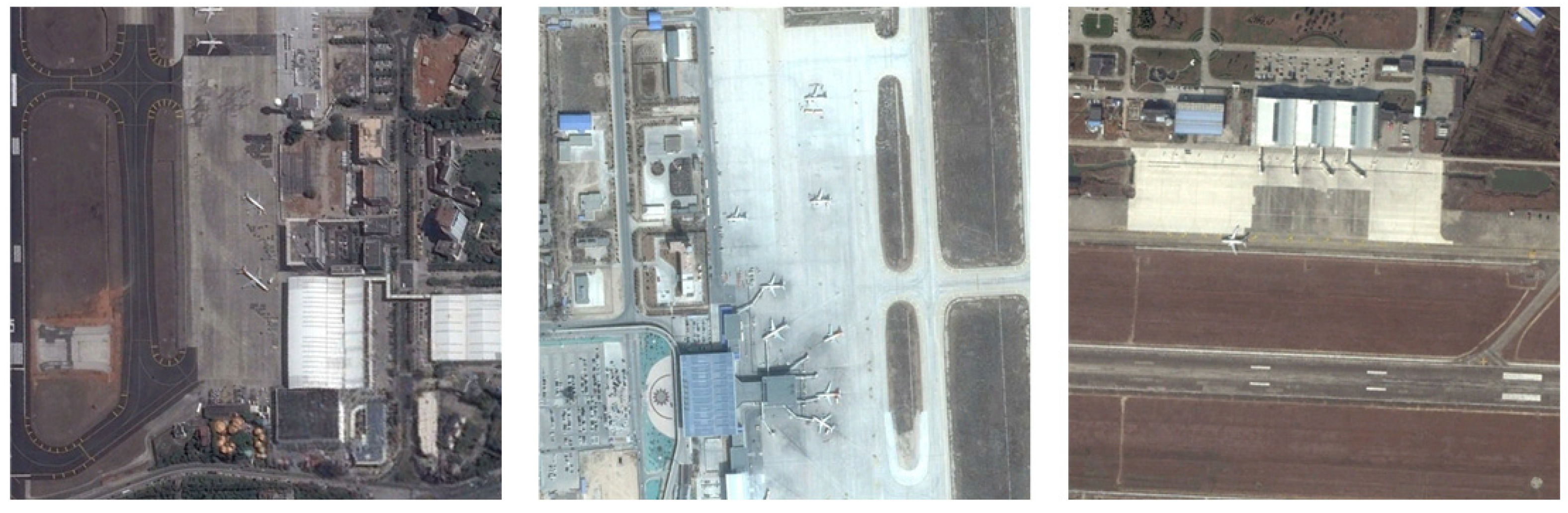
Figure 1. The challenge of significant target scale variations in remote sensing images. From left to right, these “Airport” scenes demonstrate extreme scale differences, featuring a runway spanning the entire image and an aircraft occupying only a few pixels. Images are from the AID [9].
Remotesensing 18 01235 g001
Figure 2. The challenge of complex background interference. From left to right, these “School” scenes illustrate severe visual disturbances caused by various buildings, seawater, and vegetation. Images are from the AID [9].
Remotesensing 18 01235 g002
Figure 3. The influence of spatial layout and structural distribution. From left to right, the images show a “School” scene where buildings and vegetation are closely arranged, a “DenseResidential” scene, and a “SparseResidential” scene. This highlights how scenes can have similar structural distributions but different spatial layouts. Images are from the AID [9].
Remotesensing 18 01235 g003
Figure 4. Overall architecture diagram of MS-DARNet.
Remotesensing 18 01235 g004
Figure 5. Comparison of the Mish activation function used in this paper with other mainstream activation functions (ReLU, Leaky ReLU, Swish, GELU). The main graph shows the curve shapes of each function on the input interval [−4, 4]. The embedded graph at the lower right corner provides a magnified view of the negative interval [−2.5, −0.5].
Remotesensing 18 01235 g005
Figure 6. Structure of the MDFE module.
Remotesensing 18 01235 g006
Figure 7. Sampling schematic diagram of convolutional kernels with different dilation rates in the MDFE module. The colored squares represent the effective weight positions of the 3 × 3 convolutional kernels, and the light-colored background area represents the corresponding receptive field range. (a) d = 2: The expansion rate is 2, and the sampling point intervals are relatively small, which is used to extract local texture features. (b) d = 4: The expansion rate is 4, and the sampling point intervals increase, which is used to cover a larger spatial structure without adding parameters.
Remotesensing 18 01235 g007
Figure 8. Structure of the CPAA module.
Remotesensing 18 01235 g008
Figure 9. Schematic diagram of the bionic mapping between human visual selective perception and the SCAB module. Left: The mechanism of the human visual system, in which Foveal Vision focuses on small targets (such as aircraft) to capture clear local details, while Peripheral Vision covers a wide background area to perceive the global environmental context. Right: The bionic implementation of the SCAB module adopts a large kernel decomposition strategy to simulate the biological vision mechanism. It uses a 5 × 5 convolution to simulate center focusing for extracting ontological features and a 7 × 7 dilation convolution with a dilation rate of 3 to simulate peripheral perception for aggregating long-distance context information. The combination of the two effectively suppresses complex background noise.
Remotesensing 18 01235 g009
Figure 10. Visual display of spatial position feature information. (a) Original image. (b) The result of traditional global average pooling (GAP). This result was generated by forcibly compressing two-dimensional features into a single numerical value, causing the complete collapse of the spatial structure information of the target and making it impossible to perceive the specific distribution pattern of the target. (c) The results of the PLAB branch we proposed. This result is achieved by aggregating features along the horizontal and vertical directions respectively to generate a pair of direction-aware vectors containing precise coordinate information. Subsequently, these two vectors are reconstructed back to the two-dimensional space through the outer product, presenting a clear positioning response and precisely locking the coordinate positions of all targets.
Remotesensing 18 01235 g010
Figure 11. Grad-CAM visualization of the Context-Position Aware Attention (CPAA) module on a “SparseResidential” scene. (a) Original input image. (b) Attention heatmap generated by the baseline network without CPAA, exhibiting dispersed focus on background elements (such as swimming pool and vegetation). (c) Attention heatmap generated by the proposed model equipped with CPAA, demonstrating highly concentrated and precise localization on the primary architectural structures.
Remotesensing 18 01235 g011
Figure 12. Comparison of probability distributions between standard One-Hot encoding and label smooth regularization.
Remotesensing 18 01235 g012
Figure 13. Confusion matrix on the AID.
Remotesensing 18 01235 g013
Figure 14. Confusion matrix on the NWPU-RESISC45 dataset.
Remotesensing 18 01235 g014
Figure 15. Confusion matrix on the RSD-WHU46 dataset.
Remotesensing 18 01235 g015
Figure 16. Systemic sensitivity analysis of classification accuracy (OA, %) with respect to different dilation rate combinations d 1 , d 2 across AID, NWPU-RESISC45, and RSD-WHU46 datasets.
Remotesensing 18 01235 g016
Figure 17. Performance comparison of different loss functions on the long-tailed RSD-WHU46 dataset, evaluated by Overall Accuracy (OA) and F1-scores of representative Head/Tail classes.
Remotesensing 18 01235 g017
Figure 18. Ablation study of different activation strategies in the MDFE module. The grouped bar chart compares the OA of uniform activation schemes (ReLU, SeLU, Mish) and mixed strategies across the AID, NWPU-RESISC45, and RSD-WHU46 datasets. The proposed mixed strategy (Mish SeLU, highlighted in hatched bars) consistently achieves the highest performance by effectively guiding gradient flow during initial feature extraction and stabilizing distribution variance after multi-scale fusion.
Remotesensing 18 01235 g018
Figure 19. Ablation study of the large-kernel decomposition strategy in the CPAA module. The dual-axis chart illustrates the trade-off between classification accuracy (bars, left axis) and parameter complexity (red line, right axis) under different convolutional kernel configurations. The proposed bionic configuration ( 5 × 5 + 7 × 7 ,   d = 3 ) achieves the optimal balance, maximizing accuracy while maintaining a highly compact parameter footprint compared to baseline small kernels or excessively large combinations.
Remotesensing 18 01235 g019
Figure 20. Visual similarity analysis of the most confusable category pairs. Representative samples from AID (Desert vs. BareLand), NWPU-RESISC45 (Railway vs. Railway Station), and RSD-WHU46 (Square vs. Dock) demonstrate extreme inter-class homogeneity. These pairs share highly similar underlying textures (such as sand), identical macroscopic contexts (such as parallel tracks), or flat, paved geometric surfaces, lacking distinct architectural boundaries for differentiation.
Remotesensing 18 01235 g020
Figure 21. Diagnostic Grad-CAM visualizations on representative failure cases. The baseline ResNet-50 struggles to form coherent perceptions across all challenging scenes, exhibiting scattered blobs (Desert), fragmented and misaligned focus (Railway), or massive diffuse activations (Square). In contrast, the proposed MS-DARNet extracts highly structured spatial patterns: a highly concentrated focal point in the Desert, distinct parallel activation lines tracking the rails in the Railway, and a precise ‘T’-shaped geometric outline in the Square. This demonstrates CPAA’s superior structural capture capability, though it is forced to anchor on non-discriminative shared geometries in the absence of defining semantic landmarks.
Remotesensing 18 01235 g021
Figure 22. t-SNE visualization of deep feature embeddings for the most challenging category pairs. Across all three datasets, the high-dimensional feature distributions exhibit substantial overlap and severe boundary entanglement, substantiating the inherent mathematical difficulty in establishing sharp decision hyperplanes for highly homogenized scenes.
Remotesensing 18 01235 g022
Table 1. Details of the three Datasets.
DatasetsClassImage NumberImage Per-ClassSizeTraining Ratio
AID3010,000220 420 600 × 600 20%, 50%
NWPU454531,500 700 256 × 256 10%, 20%
RSD-WHU4646117,000500 3000-10%, 20%
Table 2. Experimental Environment and Parameter Settings.
ItemContent
ProcessorIntel(R) Xeon(R) Platinum 8470Q
Memory90 GB
Operating systemUbuntu 22.04
Hard disk80 GB (30 GB System + 50 GB Data)
GPURTX 5090 (32 GB)
Python3.12
PyTorch2.8.0
CUDA12.8
Learning rate2 × 10−5
Momentum0.9
Num workers2
Batch16
Grad clip5
Random seed42
OptimizerSGD
LR scheduleCosine Annealing
Warmup epochs5
Weight decay5 × 10−4
Epoch200
Table 3. Classification accuracy (%) of our model and other models when the training ratio on the AID is 20% and 50% respectively. Methods marked with an asterisk (*) were re-implemented by us under the exact same data split, augmentation, and training protocol for fair comparison.
Models20%50%
CaffeNet [9]86.72 ± 0.4588.91 ± 0.26
VGG–VD–16 [9] *87.81 ± 0.1890.56 ± 0.26
GoogLeNet [9]83.27 ± 0.3685.67 ± 0.55
Fusion by addition [60]-91.79 ± 0.26
TEX–Net–LF [61]93.91 ± 0.1595.66 ± 0.17
LiG with RBF kernel [48]94.32 ± 0.2396.22 ± 0.25
APDC-Net [62]88.61 ± 0.2592.21 ± 0.26
VGG19 [63] *89.23 ± 0.2693.03 ± 0.31
ResNet50 [64] *92.76 ± 0.2396.35 ± 0.11
ResNet50 + SE [64]92.77 ± 0.1895.84 ± 0.22
ResNet50 + CBAM [64]92.29 ± 0.1595.38 ± 0.16
ResNet50 + HFA [64]93.11 ± 0.2095.86 ± 0.15
InceptionV3 [63]92.65 ± 0.1994.97 ± 0.22
DenseNet121 [65]92.91 ± 0.2594.65 ± 0.25
DenseNet169 [65]92.39 ± 0.3593.46 ± 0.27
Two–stream deep fusion Framework [22]92.42 ± 0.3894.62 ± 0.27
Two–stage deep feature Fusion [22]-93.87 ± 0.35
LCPP [64]91.12 ± 0.3593.35 ± 0.35
RSNet [64]94.62 ± 0.2796.78 ± 0.56
SPG–GAN [64]92.31 ± 0.1794.53 ± 0.38
VGG16 + CBAM [48]91.91 ± 0.3595.53 ± 0.07
VGG16 + SE [48]91.98 ± 0.3195.45 ± 0.19
VGG16 + HFAM [48]92.06 ± 0.1695.78 ± 0.21
LGML + Deep Learning [66]94.79 ± 0.2897.72 ± 0.25
LGRIN [67]94.74 ± 0.2397.65 ± 0.25
LG-DCN [49] *94.78 ± 0.21 96.98 ± 0.15
CLGDL [50] *92.95 ± 0.2595.38 ± 0.15
LGLMNet [68] *93.70 ± 0.1395.29 ± 0.18
Proposed95.12 ± 0.2897.78 ± 0.17
Table 4. Classification accuracy, recall rate and F1 score of our model for each category on the AID.
Class NamePrecisionRecallF1 Score
Airport96.98%98.06%97.51%
Bare Land93.48%97.10%95.25%
Baseball Field98.64%99.09%98.87%
Beach99.01%99.75%99.38%
Bridge98.05%97.78%97.91%
Center95.82%96.92%96.37%
Church97.48%96.67%97.07%
Commercial98.03%99.43%98.72%
Dense Residential98.77%98.05%98.41%
Desert98.25%93.67%95.90%
Farmland97.56%97.30%97.43%
Forest99.60%99.20%99.40%
Industrial96.98%98.97%97.97%
Meadow99.29%100.00%99.64%
Medium Residential98.62%98.28%98.45%
Mountain98.84%100.00%99.42%
Park98.79%93.14%95.88%
Parking100.00%99.49%99.74%
Playground98.64%97.84%98.24%
Pond98.57%98.33%98.45%
Port99.46%97.11%98.27%
Railway Station99.19%94.23%96.65%
Resort94.90%96.21%95.55%
River97.10%98.05%97.57%
School95.71%96.67%96.19%
Sparse Residential98.03%99.67%98.84%
Square93.90%97.88%95.85%
Stadium98.62%98.28%98.45%
Storage Tanks98.88%98.06%98.47%
Viaduct99.05%99.76%99.41%
Table 5. Classification accuracy (%) of our model and other models on the NWPU-RESISC45 dataset at 10% and 20% training ratios. Methods marked with an asterisk (*) were re-implemented by us under the exact same data split, augmentation, and training protocol for fair comparison.
Models10%20%
APDC-Net [62]85.94 ± 0.2287.84 ± 0.26
CNN + GCN [70]90.75 ± 0.2192.87 ± 0.13
LG-Sigmoid [71]90.19 ± 0.1193.21 ± 0.12
LG-RBF [67]90.23 ± 0.1393.25 ± 0.12
LGRIN [67]91.91 ± 0.1594.43 ± 0.16
VGG19 [63] *82.74 ± 0.2285.07 ± 0.27
GoogLeNet [9]82.46 ± 0.1285.36 ± 0.17
MobileNet V2 [72]89.83 ± 0.1692.16 ± 0.15
ResNet50 [64] *87.83 ± 0.2190.27 ± 0.11
SE-MDPMNet [73]91.80 ± 0.0794.11 ± 0.03
Contourlet-CNN [74]85.93 ± 0.5189.57 ± 0.45
Inception-V3 [63]85.46 ± 0.3387.75 ± 0.43
Xception [72]81.64 ± 0.3284.79 ± 0.26
EfficientNet [72]78.57 ± 0.1581.83 ± 0.15
SCC-CNN [75]92.02 ± 0.5094.39 ± 0.16
LCNN-GWHA [76]92.24 ± 0.1294.26 ± 0.25
RS-DARTS [77]85.73 ± 0.2689.15 ± 0.36
LCNN-CMGF [71]92.53 ± 0.5694.18 ± 0.35
DF-CNN [10] *89.88 ± 0.3794.44 ± 0.35
RSMamba [46] *91.59 ± 0.4493.45 ± 0.37
STMSF [44] *85.69 ± 0.2187.28 ± 0.23
LG-MSMA [48] *92.07 ± 0.2694.17 ± 0.13
Proposed92.31 ± 0.1294.53 ± 0.23
Table 6. The precision, recall and F1 score of our model for each category on the NWPU-RESISC45 dataset.
Class NamePrecisionRecallF1 Score
Airplane0.95720.99000.9733
Airport0.91020.95570.9324
Baseball Diamond0.97050.98570.9780
Basketball Court0.94320.94860.9459
Beach0.96460.97430.9694
Bridge0.97020.97710.9737
Chaparral1.00000.99290.9964
Church0.91900.84290.8793
Circular Farmland0.97320.98430.9787
Cloud0.96930.99290.9809
Commercial Area0.95280.89430.9226
Dense Residential0.96060.94140.9509
Desert0.96360.98290.9731
Forest0.95980.98860.9740
Freeway0.94210.97570.9586
Golf Course0.98290.98290.9829
Ground Track Field0.99850.94710.9721
Harbor0.99130.98000.9856
Industrial Area0.93080.96140.9459
Intersection0.97400.96140.9676
Island0.96480.98000.9724
Lake0.96110.95290.9570
Meadow0.97700.97000.9735
Medium Residential0.96450.89140.9265
Mobile Home Park0.98710.98000.9835
Mountain0.98250.96000.9711
Overpass0.94830.97000.9590
Palace0.88000.88000.8800
Parking Lot0.99420.97430.9841
Railway0.98260.89000.9340
Railway Station0.88110.92140.9008
Rectangular Farmland0.95120.94710.9492
River0.91930.96000.9392
Roundabout0.97290.97290.9729
Runway0.96520.95140.9583
Sea Ice0.98860.98860.9886
Ship0.95060.96140.9560
Snowberg0.98400.96860.9762
Sparse Residential0.91900.97290.9452
Stadium0.97430.97570.9750
Storage Tank0.97670.95710.9668
Tennis Court0.96480.97860.9716
Terrace0.93530.97000.9523
Thermal Power Station0.90040.95570.9272
Wetland0.95930.90860.9332
Table 7. Classification accuracy (%) of our model and other models at 10% and 20% training rates on the RSD-WHU46 dataset. Methods marked with an asterisk (*) were re-implemented by us under the exact same data split, augmentation, and training protocol for fair comparison.
Model10%20%
AlexNet [78]80.62 ± 0.3583.56 ± 0.26
GoogLeNet [9]81.35 ± 0.2584.23 ± 0.33
ResNet50 [64] *86.45 ± 0.2789.12 ± 0.33
SE-ResNet50 [79]92.27 ± 0.2593.43 ± 0.33
VGG16 [48] *85.97 ± 0.2188.03 ± 0.19
Inception-V3 [63]87.85 ± 0.3188.72 ± 0.25
DenseNet [65]88.77 ± 0.3589.87 ± 0.33
Xception [72]88.63 ± 0.3789.93 ± 0.35
MobileNet V2 [72]85.59 ± 0.3588.13 ± 0.36
SqueezeNet1.0 [80]82.73 ± 0.1685.26 ± 0.28
ShuffleNet-1.5x [81]83.67 ± 0.1985.11 ± 0.16
EfficientNet-B0 [82]86.35 ± 0.2288.67 ± 0.19
DCMNet(Terminal) [50]88.75 ± 0.2689.86 ± 0.25
DCMNet(Cloud) [50]90.56 ± 0.2791.78 ± 0.25
DCNNet(Terminal) [83]88.53 ± 0.2589.79 ± 0.22
LCPP [64] 90.53 ± 0.1192.66 ± 0.31
CLGDL [50] *91.95 ± 0.2394.21 ± 0.13
Proposed92.06 ± 0.0894.55 ± 0.23
Table 8. The precision, recall and F1 score of our model for each category on the RSD-WHU46 dataset.
Class NamePrecisionRecallF1 Score
Airplane0.98050.99560.9880
Airport0.96020.97570.9679
Artificial Dense Forest Land0.93080.86220.8952
Artificial Sparse Forest Land0.92180.88920.9052
Bare Land0.92110.93330.9272
Basketball Court0.91970.94850.9339
Blue Structured Factory Building0.94010.98910.9640
Building0.86440.88610.8751
Construction Site0.86570.87980.8727
Cross River Bridge0.99110.98810.9896
Crossroads0.97390.97390.9739
Dense Tall Building0.93390.92170.9278
Dock0.98710.97250.9797
Fish Pond0.97550.99170.9835
Footbridge0.96930.96440.9668
Graff0.93440.94680.9405
Grassland0.94960.93400.9417
Irregular Farmland0.95220.97450.9632
Low Scattered Building0.96110.96380.9624
Medium Density Scattered Building0.91130.88420.8975
Medium Density Structured Building0.95780.93800.9478
Natural Dense Forest Land0.91430.94890.9313
Natural Sparse Forest Land0.94130.96870.9548
Oil Tank0.91510.98340.9480
Overpass0.97830.96270.9704
Parking Lot0.91240.97820.9442
Plastic Greenhouse0.95001.00000.9744
Playground0.96260.96260.9626
Railway0.98010.95280.9663
Red Structured Factory Building0.98420.97540.9798
Refinery0.91880.87970.8988
Regular Farmland0.94400.94590.9450
Scattered Blue Roof Factory Building0.91860.93870.9286
Scattered Red Roof Factory Building0.95680.95680.9568
Sewage Plant-Type-One0.92860.97500.9512
Sewage Plant-Type-Two0.98330.92190.9516
Ship0.98250.99330.9879
Solar Power Station0.97380.98240.9781
Sparse Residential Area0.92920.96870.9485
Square0.98130.84680.9091
Steelworks0.90130.93620.9184
Storage Land0.98110.98730.9842
Tennis Court0.95930.91380.9360
Thermal Power Plant0.87960.88890.8842
Vegetable Plot0.93440.92360.9290
Water0.98500.97040.9777
Table 9. Evaluation of model performance, theoretical complexity, and physical deployment metrics. Methods marked with an asterisk (*) were re-implemented by us under the exact same experimental settings for fair comparison.
ModelsOA (%)Parameters (M)GMACs (G)Latency (ms)FPSMemory (MB)
ResNet50 [64] *96.3525.611.855512.580250
CaffeNet [9] 89.5360.973.653210.298280
MobileNet V2 [72] *95.963.500.34514.223865
GoogLeNet [9] 86.397.000.75008.5118130
SE-MDPMNet [73] 97.145.170.98439.8102145
VGG-VD-16 [84] 89.64138.367.750028.535550
Inception-V3 [63]95.0745.372.435618.554220
LGRIN [67]97.654.630.49336.515385
LG-DCN [49] *96.9813.3121.321615.465180
LGLMNet [68]95.292.61.08007.311595
Proposed97.782.50.59407.8128110
Table 10. Ablation Results of Key Modules across three datasets (Overall Accuracy, %).
Key BlockAIDNWPU45RSD-WHU46
MDFE89.6486.1286.55
CPAA95.3391.8592.10
MDFE and CPAA97.7894.5394.55
Table 11. Ablation Results of the Attention Mechanism Branches (Overall Accuracy, %).
Attention Mechanism BranchAIDNWPU45RSD-WHU46
PLAB Only94.5790.7591.20
SCAB Only96.4593.1292.85
PLAB and SCAB97.7894.5394.55
Table 12. Ablation Results of multi-scale feature fusion in stages (Overall Accuracy, %).
Stage—Wise Multi—Scale Feature FusionAIDNWPU45RSD-WHU46
Stage 191.9387.5088.10
+Stage 293.3989.1089.60
+Stage 396.5292.8093.10
+Stage 497.7894.5394.55
Table 13. Ablation Results of convolutional kernel design and receptive field expansion strategy.
Convolutional Kernel StrategyParameters (M)AID (%)NWPU45 (%)RSD-WHU46 (%)
Standard Small Convs2.3593.8290.1590.45
Standard Large Convs14.7296.4592.8593.15
Proposed2.5097.7894.5394.55
Table 14. Sensitivity analysis of other structural configurations on the AID.
Configuration TypeSettingOA (%)Parameters (M)
Number of MDFE Branches1 Branch ( d = 2 )93.821.80
2 Branches ( d = 2 ,   4 ) [Proposed]97.782.50
3 Branches ( d = 2 ,   4 ,   6 )97.803.25
Label Smoothing ϵ ϵ = 0.05 97.55-
ϵ = 0.10 [Proposed]97.78-
ϵ = 0.20 97.21-
STEM NormalizationPost-activation (Conv BN Mish)97.35-
Pre-activation (BN Conv Mish) [Proposed]97.78-
Disclaimer/Publisher’s Note: The statements, opinions and data contained in all publications are solely those of the individual author(s) and contributor(s) and not of MDPI and/or the editor(s). MDPI and/or the editor(s) disclaim responsibility for any injury to people or property resulting from any ideas, methods, instructions or products referred to in the content.