Detecting Woody Plant Cover in the Foothills Parkland and Montane Ecoregions of Southern Alberta

Highlights

What are the main findings?

• Woody plant response to environmental factors varied by species;
• PlanetScope’s yellow band had the highest ability to separate woody cover stages of the investigated bands.

What are the implications of the main findings?

• Responses to shrub encroachment need to consider the unique characteristics of woody plant species.
• The yellow band could be beneficial in future investigations into woody plant encroachment.

Abstract

Grasslands globally are threatened by loss and degradation as shifting factors in climate and management put them at risk. These grassland ecosystems support local economies and are a center of biodiversity, which makes understanding the risks that affect them key to effectively protecting them. One major risk to grasslands is woody plant encroachment, and reliable management hinges on understanding its patterns. A major challenge of woody plant encroachment is detecting it at early stages (<20% cover). This study investigated the utility of a combination of environmental features and remotely sensed data for differentiating varying levels of woody plant encroachment in a montane Canadian grassland. The response of woody species to environmental factors including slope and available moisture varied by individual species. As in past studies, it was challenging to separate the early stages of encroachment using base spectral bands or NDVI, even with the use of higher-resolution satellite imagery. Bands in the yellow and red wavelength regions both showed promise for shrub detection, providing more between band separability and key modeling components. The spatial resolution and band combinations used here were able to model woody plant cover levels, helping to facilitate the implementation of effective management in combating woody plant encroachment.

1. Introduction

Grasslands around the globe are threatened by area loss and quality reduction, with few large intact grasslands remaining [1]. The World Wildlife Fund reported 32 million acres of North American grassland having been converted since 2012 [2]. Conversion and subsequent area loss can be the result of expansion of agriculture and urban areas. Quality reduction and its causes can be more complex to measure. Factors such as poor management, climate change, invasive species, overgrazing, and woody plant encroachment (WPE) can all contribute to decreases in quality [1,2,3,4,5]. The negative impacts of WPE are a cause of concern from both ecological and economic perspectives. While the measurement of productivity and ecosystem services is complex, the threat that WPE poses to grassland native species is clear [6,7,8]. It is within the complex question of productivity that the concerns for ranchers lie. Reduction in forage quality can significantly impact grazing operations [9,10,11]. This is a concern for the many grazing operations found in southern Alberta, where, as of January 2026, 21,050 operations have reported having cattle [12]. The impacts of WPE on grasslands are of serious concern, and understanding this phenomenon is key to addressing its impacts.

Broadly, WPE can be understood as an increase in woody plants in grasslands beyond typical cover levels [13,14]. While historically, woody plants in grasslands have been limited by disturbance, including fire and grazing, shifts in these regimes have increased risk to and degradation of grassland ecosystems [4,13,15,16,17]. The suppression of fire is understood to be a contributing factor in the degradation of grassland ecosystems [10,15,16]. There have been rising movements to reintroduce fire to grassland ecosystems to improve their health and manage problems like WPE [4,7,10,18,19,20,21]. The loss of historic grazing patterns is another contributor to the degradation of grasslands, especially in North America [11,17,20]. Determining how to effectively apply modern management techniques relating to these disturbance factors is the focus of many current grassland studies [7,22,23]. The ability of land managers to apply these techniques to best counter issues like WPE is, in part, reliant on understanding the patterns of these issues [24,25]. Determining these patterns is where the use of remote sensing technologies is key.

Remotely sensed data has been used to map and manage grasslands for decades [26,27,28,29,30]. Recently, there has been an increase in investigations into woody cover in grasslands using remote sensing techniques [31,32,33,34,35]. The differences in leaf structure and phenology between grass and woody plants make it possible to use remote sensors to differentiate between these two types of cover and map significant increases in woody cover in grasslands [32]. As a progressive phenomenon, the early stages (<20%) of WPE have proven particularly challenging to monitor [36,37]. Further, investigating small shifts in this progressive change can be difficult since it may take decades for grassland to reach a high cover of woody species. The purpose of this study is to find better ways to estimate woody cover, particularly at early stages of encroachment, using remotely sensed data. Our specific objectives are to (1) evaluate the biophysical and spectral properties of woody plants at different woody cover levels in a grassland ecosystem, (2) identify the best spectral and environmental features to estimate woody cover, and (3) map woody cover at different abundance levels in the study area using the features identified in objective 2.

2. Materials and Methods

2.1. Study Area

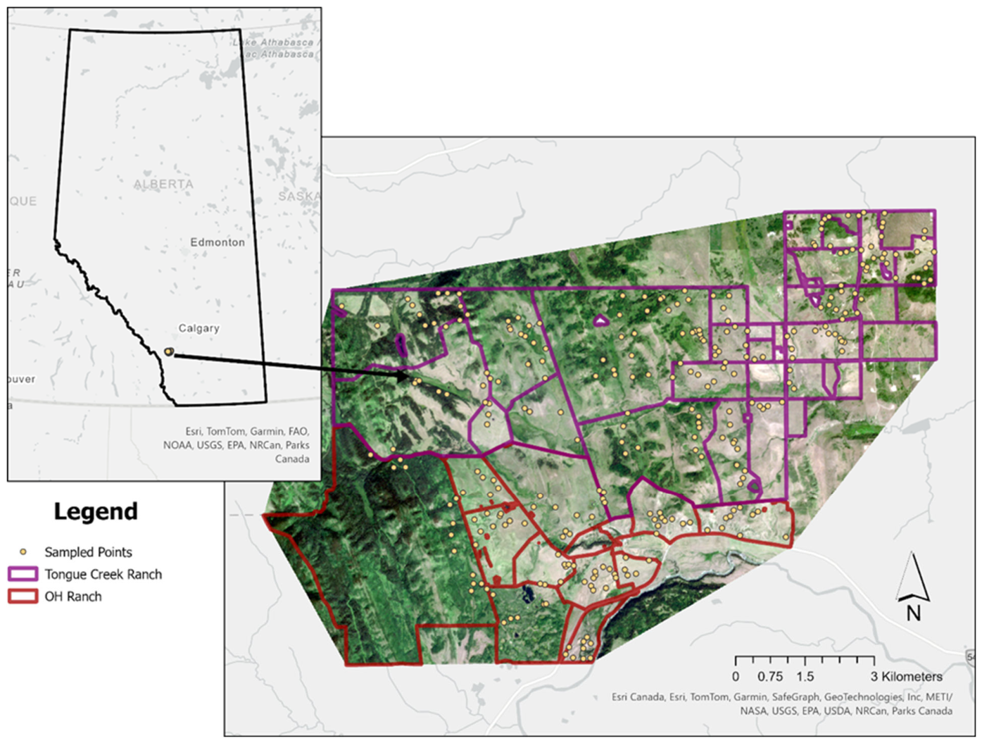
The field sampling was conducted in grasslands managed by Tongue Creek Ranch and OH Ranch, near Longview, Alberta, Canada (Figure 1). The site falls within the Foothills Fescue, Foothills Parkland, and Montane natural subregions of Alberta and covers close to 80 km² in total [38,39]. These grasslands are dominated by a mixture of mountain rough fescue (Festuca campestris), Parry oat grass (Danthonia parryi), and Idaho fescue (Festuca idahoensis), as well as a wide variety of forbs [38,40]. As both ranches are being actively managed to support livestock, there are also areas of non-native seeded pasture present. This region normally supports a range of woody species. Large woody species found on the site include trembling aspen (Populus tremuloides), balsam poplar (Populus balsamifera), white spruce (Picea glauca), and willow (Salix sp.). Smaller shrubby species such as roses (Rosa sp.), shrubby cinquefoil (Dasiphora fruticosa), red-osier dogwood (Cornus sericea), dwarf birch (Betula pumila), bearberry (Arctostaphylos uva-ursi), silverberry (Elaeagnus commutata), snowberry (Symphoricarpos sp.), saskatoon berry (Amelanchier alnifolia), raspberry (Rubus sp.), chokecherry (Prunus virginiana), and gooseberry (Ribes spp.) are also common.

The general topography comprises rolling hills on the eastern foothills of the Canadian Rockies, with some areas of steep slopes up to 49°. Steep areas of the property are primarily hills along the west side and coulees on the south side. The soils are primarily Orthic Black Chernozems, with potential for some Dark Gray Chernozems in higher-elevation areas [38,40]. The natural subregions included in the study area receive an annual average precipitation of 414–500 mm [42,43].

The site has a 140-year history of ranching, and land managers prioritize sustainable management to conserve the native grassland ecosystems [39]. Management is split between two operations, OH Ranch and Tongue Creek Ranch, with some varying levels and timings of cattle grazing occurring across the entire site. The public land portions of the OH ranch were designated as Heritage Rangeland under the Wilderness Areas, Ecological, Natural Areas, and Heritage Rangelands Act in 2008. In 2009, the public land holdings of the OH Ranch were placed under conservation easement to ensure that the grassland remains intact for grazing and wildlife habitat. This restricts the land managers from using prescribed fire or herbicides in their management of those areas.

2.2. Field Data Collection and Processing

An initial set of 1000 potential ground reference points was generated using the Create Random Points tool in ArcGIS Pro (Version 3.3.0), in a stratified random distribution. Stratification was based on slope and aspect, derived from provincial 25 m DEM data [44]. Slope values were separated into five categories using the quantile method to create ranges representative of the rate of occurrence of various slopes. Aspect was divided into four categories representing each of the cardinal directions. Points were stratified by these factors to capture the impact of topographic variation on woody plant cover. Underlying moisture conditions determined by soil and topography are stable mapped factors impacting areas of woody cover [45,46]. During fieldwork, the numbers of samples from each category combination, totaling 20 unique categories present on site from each intersection of slope and aspect categories, were tracked (

Table 1. Sample distribution based on topographic categories, where the first number represents a slope value starting at 1 for low slope angles and increasing as slope angles increase, and the second number represents aspect values, with north being 1 and the clockwise sequential cardinal directions following.

Topographic Category	1.1	1.2	1.3	1.4	2.1	2.2	2.3	2.4	3.1	3.2	3.3	3.4	4.1	4.2	4.3	4.4	5.1	5.2	5.3	5.4
# Sampled	12	32	14	9	15	23	14	9	16	20	11	13	10	14	10	13	9	16	9	14

). This ensured that approximately equivalent proportions of points were sampled from each category, according to the proportion of the total study area each represented. Samples were collected from across the full landscape, totaling 290 sampled points. The remaining points from the initial 1000 potential generated were excluded due to time and accessibility constraints.

Sampling was done in clusters to allow efficient movement of the field crew between sampling plots across each field on the two ranches. Clusters were selected to (1) ensure sampling coverage across the full landscape and (2) ensure representative sampling of each slope and aspect category. A Trimble Geo 7X GPS (~52 cm accuracy) was used to navigate to each field site and a 10 m × 10 m site was established. Five 1 m × 1 m quadrats were sampled at each field site [36]. Each quadrat was assessed for total percent cover of grass, forbs, litter, bare ground, and individual woody plant species at 1% intervals from 0–5% and 95–100% cover and 5% intervals from 5–95% cover [47]. Measurements from the five quadrats were averaged to create a site representative sample. In total, after removing outliers and errors, 286 points were used for analysis of the 290 sampled points.

Woody cover was divided into subcategories of total tree cover, total shrub cover, and some common individual woody species. To understand the progressive change in woody cover, we divided woody cover into 9 categories based on the intervals used to assess cover in the field (

Table 2. Average cover by type for each woody cover category with the total study area average and standard deviation at the bottom.

	Woody Cover	% Cover Range	# of Samples	Grass	Forbs	Litter	Bare Ground	Total Woody	Total Tree	White Spruce	Trembling Aspen	Balsam Poplar	Total Shrub	Total Willow	Total Rose
Woody Cover Category	0	[0]	55	37.3	14.1	34.4	10.8	0	0	0	0	0	0	0	0
	1	(0, 5]	53	26.9	16.8	40.2	8.5	2.1	0.1	0	0.0	0.1	2.0	0.1	1.2
	2	(5, 10]	36	21.1	21.1	35.9	10.8	7.4	0.4	0	0.3	0.1	7.0	0.8	4.0
	3	(10, 15]	24	18.8	16.6	35.5	10.5	12.8	1.5	0	0.2	1.3	11.3	2.2	4.7
	4	(15, 25]	28	25.5	20.0	24.0	7.8	19.8	2.4	0	1.2	1.2	17.4	6.7	6.3
	5	(25, 40]	22	17.0	15.7	25.7	4.8	32.1	2.6	0.5	0.5	1.6	29.5	10.3	9.2
	6	(40, 60]	27	14.3	14.6	15.3	3.2	48.7	21.8	10.6	7.9	3.4	26.9	13.0	4.6
	7	(60, 90]	25	5.5	5.3	5.7	1.8	74.5	50.1	28.0	18.4	3.6	24.4	16.2	4.7
	8	(90, 100]	16	0.1	0.4	0.5	0.2	98.2	90.5	49.5	17.1	23.9	7.7	7.4	0.2
		Total		22.0 (16.0)	14.9 (11.8)	27.9 (19.1)	7.5 (11.2)	23.4 (29.3)	12.1 (27.3)	6.3 (19.9)	3.5 (13.3)	2.4 (11.6)	11.3 (11.3)	4.8 (13.0)	3.3 (6.0)

). We used finely divided categories so that we could detect patterns in early encroachment and cover increases.

2.3. Environmental Data Acquisition and Processing

Other environmental factors including incoming solar radiation and Topographic Wetness Index (TWI) values were considered alongside the slope and aspect effects [48]. Incoming solar radiation and TWI were calculated to account for the broad factors of solar energy and available water in plant growth. The provincial DEM data was used to calculate TWI using Equation (1). Solar radiation was calculated with the ArcGIS Pro Raster Solar Radiation tool, using the provincial DEM data and assuming standard overcast sky conditions for the month of July.

$$TWI=ln{\displaystyle \frac{\alpha }{\tan \beta }},$$

(1)

where α measures the area upslope that drains through a point and tanβ is the slope of the point [49].

2.4. Remotely Sensed Data Processing

In order to increase our ability to detect early-stage, low-abundance patches of woody plants, PlanetScope Scene 8-band surface reflectance imagery (3 m resolution) from the SuperDove flock was acquired matching the time of field sampling. For our initial analysis, the spectral band data was extracted using 3 × 3 bilinear interpolation to match the spatial parameters of our field sample points.

Table 3. PlanetScope sensor bands.

Band	Name	Wavelength Range (nm)
B1	Coastal Blue	431–452
B2	Blue	465–515
B3	Green 1	513–549
B4	Green	547–583
B5	Yellow	600–620
B6	Red	650–680
B7	Red Edge	697–713
B8	NIR	845–885

Source: Planet Labs “PlanetScope” [50].

shows the 8-band configuration in the PlanetScope imagery. In addition to the original imagery, several spectral vegetation indices were calculated to account for Leaf Area Index (LAI), photosynthetic activity, and chlorophyll content (

Table 4. Vegetation indices and equations used for model development.

VI	Equation	Plant Characteristics	References
ryNDVI (Red–Yellow Normalized Difference Vegetation Index)	${\displaystyle \frac{\left(Red-Yellow\right)}{\left(Red+Yellow\right)}}$	Developed to reflect the value of the yellow band in differentiating woody cover categories, and the difficulties that the NIR posed in that same investigation	This is a newly proposed index; it has similarities to the yellow indexes developed by [51,52]
ATSAVI (Adjusted Transformed Soil-Adjusted Vegetation Index)	$a{\displaystyle \frac{NIR-a·Red-b}{a·NIR+Red-a·b+x\left(1+a^2\right)}}$ where X = 0.08, a = 1.22, b = 0.03 *	Leaf Area Index (LAI), Photosynthetic Material, Soil-Adjusted	[53]
GBNDVI (Green Blue Normalized Difference Vegetation Index)	${\displaystyle \frac{NIR-\left(Green+Blue\right)}{NIR+\left(Green+Blue\right)}}$	LAI	[54]
GOSAVI (Green Optimal Soil-Adjusted Vegetation Index)	${\displaystyle \frac{NIR-Green}{NIR+Green+Yellow}}$	Chlorophyll content	[55]
NDVI (Normalized Difference Vegetation Index)	${\displaystyle \frac{NIR-Red}{NIR+Red}}$	Photosynthetically Active Biomass	[56]
RBNDVI (Red Blue Normalized Different Vegetation Index)	${\displaystyle \frac{NIR-\left(Red+Blue\right)}{NIR+\left(Red+Blue\right)}}$	LAI	[54]
WDRVI (Wide-Dynamic-Range Vegetation Index)	${\displaystyle \frac{0.1NIR-Red}{0.1NIR+Red}}$	LAI	[57]

* To create a more generalized model that would not need to be re-calibrated across sensors, generic coefficient parameters were used.

). Standard optimized coefficients were used for the new normalized index (ryNDVI), which was formulated to capture the information from the red and yellow bands.

2.5. Statistical Analysis

We examined the relationships between plant cover and environmental factors using ANOVA and regression models fit using the aov and lm functions in the R statistical package [58]. In these analyses, the response variables were plant cover values (total woody cover, species-level woody cover, and other plant life form cover coded as exact percentage values). Covers were compared between aspect categories using ANOVA, and linear regression was used to examine the relationships between cover and continuous environmental factors (slope, solar radiation, and TWI). The Tukey Test was applied post hoc to compare the cardinal directions.

2.6. Continuous Woody Cover Mapping

To develop a model to predict continuous woody cover distribution, regression analysis was applied to total woody cover with all bands, the selected vegetation indices, and environmental variables using a stepwise approach in IBM’s SPSS Statistics software. The model was fit using a stepwise approach such that at each step, variables were either added, if the variable’s F-statistic had a p-value of less than or equal to 0.05, or removed, if the variable’s F-statistic had a p-value of greater than or equal to 0.1. Adjusted R² was used to verify the accuracy of the resulting linear regression model.

Very few satellites currently in operation make use of the yellow band. Similarly, the red-edge band is not available through many satellite platforms. To accommodate the band availability of different satellite configurations, we not only developed a model of woody cover estimation with the data from the Planet data we were using in this study, but also developed models without the yellow band, and with only NDVI data and the associated red and NIR bands. The developed regression model was applied in ArcGIS Pro to map woody cover and illustrate the spatial distribution at different levels of the woody cover in the study area. The total area and percentage of woody cover at the nine stages were calculated using the resulting map product.

3. Results

The average total woody cover of the study area based on the field samples was 23.3%, with approximately half of that cover being trees (12.1%) and the other half shrubs (11.2%). In grass-dominated areas, grass cover reached a maximum of 80% with the remaining cover a mix of forbs, litter, and bare ground. The broad woody classes (total, tree, and shrub) all had a maximum cover of 100%. However, the shrub subclass only reached 100% with the inclusion of the Salix species; otherwise, the total shrub class only has a maximum of 69.6% cover. Short-statured shrubs tended to have lower total cover. As an example, Rosa sp. had a maximum cover of 57% while averaging 3.3%. Overall, the sampled woody cover ranges from being free of woody plants to having complete coverage, with the total made up of a variety of compositions and statures.

3.1. Woody Plant Cover and Biophysical Characteristics

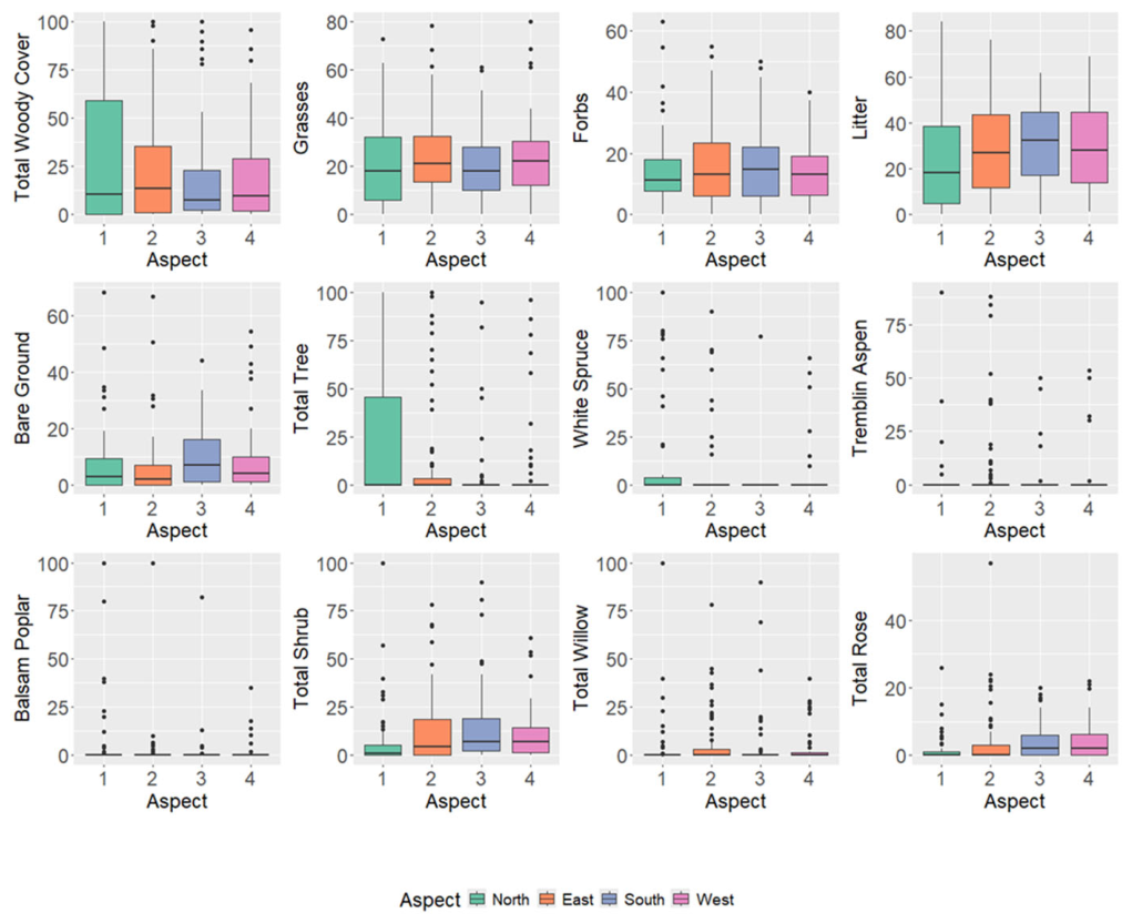
Aspect had no significant effect on overall woody cover, but total tree cover was higher on north slopes (

Table 5. ANOVA results examining impact of slope aspect on plant life form cover (%).

Cover Type	Aspect				ANOVA
	North	East	South	West	F-Value	p
Grass	20.7	23.6	19.5	23.4	1.091	0.353
Forbs	14	16.1	15	13.8	0.658	0.579
Litter	22.2	28.1	31.6	30.4	3.1	0.027 *
Bare Ground	7.6	5.4	10.1	8.6	2.453	0.064 +
Total Woody	30.4	22.8	20.5	19.6	1.813	0.145
Total Tree	23.6	10.8	5.6	8	5.787	<0.001 ***
White Spruce	15.9	4.2	1.4	3.8	7.479	<0.001 ***
Trembling Aspen	2.5	5.2	2.4	2.8	0.884	0.45
Balsam Poplar	5.2	1.4	1.8	1.4	1.739	0.159
Total Shrub	6.8	12	14.8	11.6	2.486	0.061 +
Total Willow	3.7	5.5	5.8	4	0.441	0.724
Total Rose	1.6	3.3	4	4.5	2.849	0.038 *

Note: Symbols denote significance at 0.001 (***), 0.05 (*), and 0.1 (+).

, Figure A1). The total tree cover response was primarily due to much higher white spruce cover on north aspects. Among shrubs, roses were more common on drier south and west slopes.

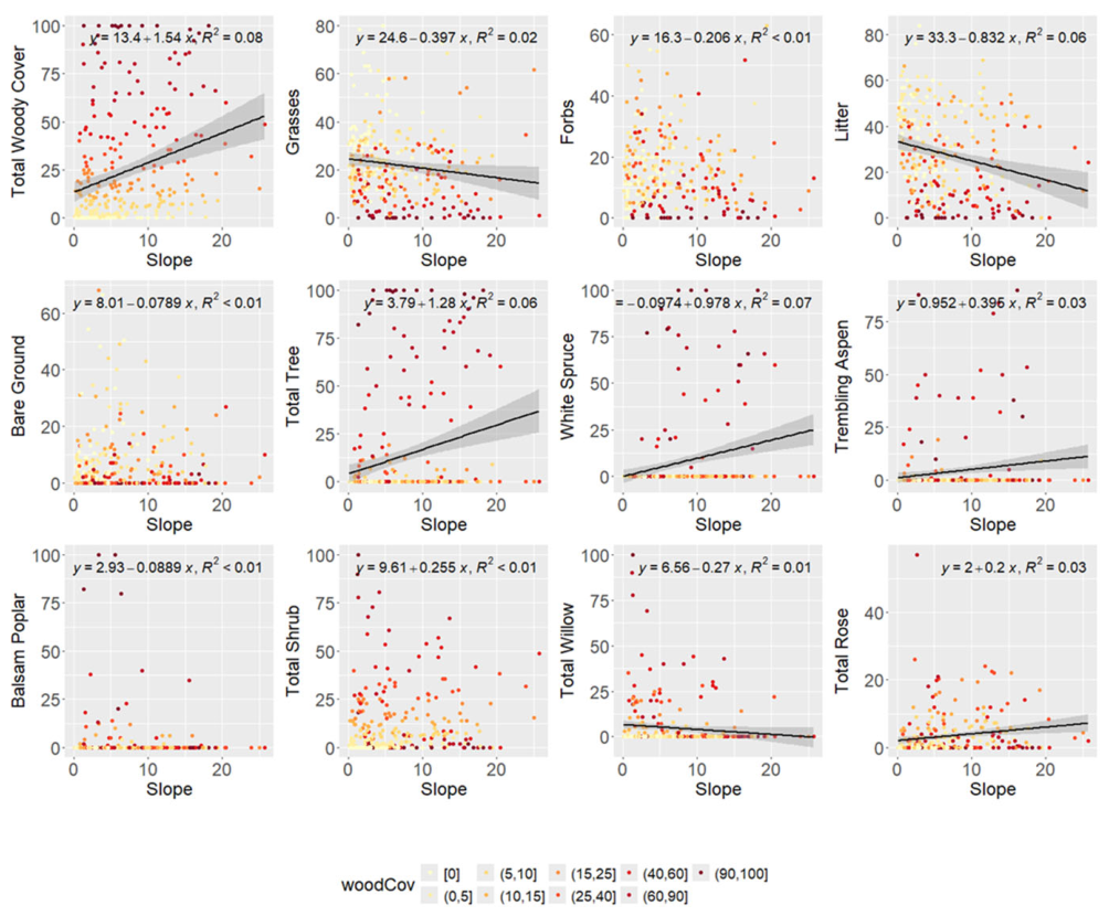
Slope had a significant effect on overall woody cover, as well as grass and litter cover (Figure A2). Total tree cover was a dominant influence, with both white spruce and trembling aspen having higher cover on steeper slopes. Overall shrub cover was not significantly affected by slope but both willow and rose cover showed some effect. While rose cover was higher as slopes increased, willow cover decreased with steeper slopes.

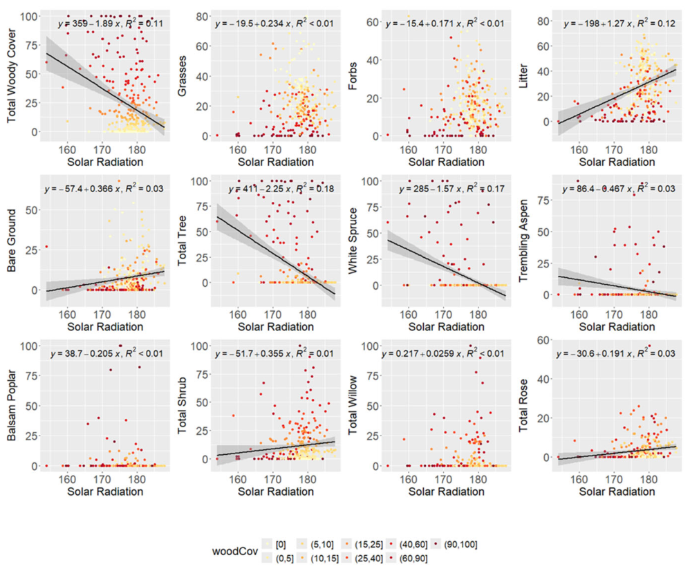
Solar radiation had a significant effect on overall woody cover, total tree, total shrub, litter, and bare ground cover (Figure A3). For the tree cover, this was caused primarily by decreased white spruce and trembling aspen with increasing solar radiation. For the total shrub cover, total rose cover increased with increasing solar radiation.

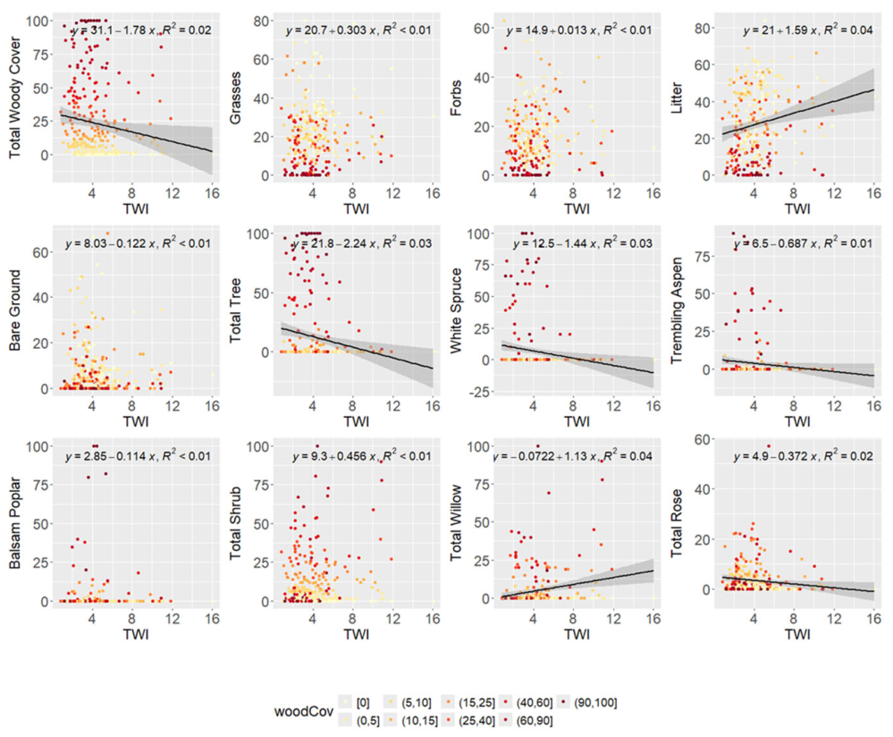
TWI had a significant effect on overall woody cover and litter cover (Figure A4). The total tree cover was influenced by both white spruce and trembling aspen, decreasing with greater wetness values. Overall shrub cover was not significantly affected by slope but both willow and rose cover showed some effect. While willow cover had a strong positive relationship with increased wetness values, rose cover decreased as wetness values increased.

3.2. Spectral Characteristics of Woody Cover Categories

Table 6. Post hoc statistics results showing woody category separability for each spectral band and NDVI, highlighting the bands with the highest ability to separate the various categories of woody cover.

	Highly Separable (***)	Moderately Separable (**)	Slightly Separable (*)
Coastal Blue	WC < 5% vs. WC > 25% WC (0–5%) vs. WC (15–25%) WC (5–15%) vs. WC > 40% WC (15–25%) vs. WC > 60%	WC = 0 vs. WC (15–25%) WC (5–10%) vs. WC (25–40%) WC (25–40%) vs. WC > 60%	WC (10–15%) vs. WC (25–40%)
Blue	WC < 5% vs. WC > 15% WC (5–10%) vs. WC > 25% WC (10–15%) vs. WC > 40% WC (15–25%) vs. WC > 60%	WC (25–40%) vs. WC > 60%	WC (5–10%) vs. WC (15–25%) WC (10–15%) vs. WC (25–40%) WC (15–25%) vs. WC (40–60%)
Green 1	WC < 5% vs. WC > 25% WC (0–5%) vs. WC (15–25%) WC (5–25%) vs. WC > 40% WC (25–40%) vs. WC > 60% WC (40–60%) vs. WC > 90%	WC = 0 vs. WC (10–25%) WC (5–15%) vs. WC (25–40%)	WC (40–60%) vs. WC (60–90%)
Green	WC < 5% vs. WC > 15% WC (0–5%) vs. WC > 40% WC (25–40%) vs. WC > 60% WC (40–60%) vs. WC > 90%	WC (25–40%) vs. WC (40–60%)	WC (5–10%) vs. WC (25–40%) WC (40–60%) vs. WC (60–90%)
Yellow	WC < 5% vs. WC > 15% WC (5–25%) vs. WC > 40% WC (25–40%) vs. WC > 60%	WC (5–10%) vs. WC (25–40%)	WC (10–15%) vs. WC (25–40%) WC (25–40%) vs. WC (40–60%) WC (40–60%) vs. WC > 90%
Red	WC < 5% vs. WC > 15% WC (5–15%) vs. WC > 40% WC (15–40%) vs. WC > 60%	WC (15–25%) vs. WC (40–60%)	WC (5–10%) vs. WC (15–40%) WC (10–15%) vs. WC (25–40%)
Red Edge	WC < 25%) vs. WC > 40% WC (40–60%) vs. WC > 60%	WC < 5% vs. WC (25–40%)	WC < 5% vs. WC (15–25%)
NIR	WC (15–40%) vs. WC > 60%	WC = 0% vs. WC (60–90%)	WC = 0% vs. WC > 90%
NDVI	WC < 5% vs. WC > 15% WC (5–10%) vs. WC > 25% WC (10–15%) vs. WC > 40%	WC (5–10%) vs. WC (15–25%) WC (10–15%) vs. WC (25–40%) WC (15–25%) vs. WC > 90%	WC (10–15%) vs. WC (15–25%) WC (15–25%) vs. WC (60–90%)

Note: Symbols denote significance at 0.001 (***), 0.01 (**), and 0.05 (*), and WC means woody cover.

summarizes the utility of spectral data for separating different woody cover categories. As identified in previous studies [36], woody cover values lower than 15% were not separable from each other under any individual bands or NDVI, making early woody plant encroachment detection challenging. However, they could be distinguished from classes with cover over 25% in most categories. The highest levels of woody cover, 60–90% and 90–100%, were not separable from each other using spectral data.

The green bands, yellow band, and red-edge band showed a strong ability to differentiate different woody cover categories. NIR showed the lowest power in detecting woody cover, which contributed to the relatively lower ability of NDVI to differentiate woody cover categories compared to the base green bands.

3.3. Modeling Total Woody Cover

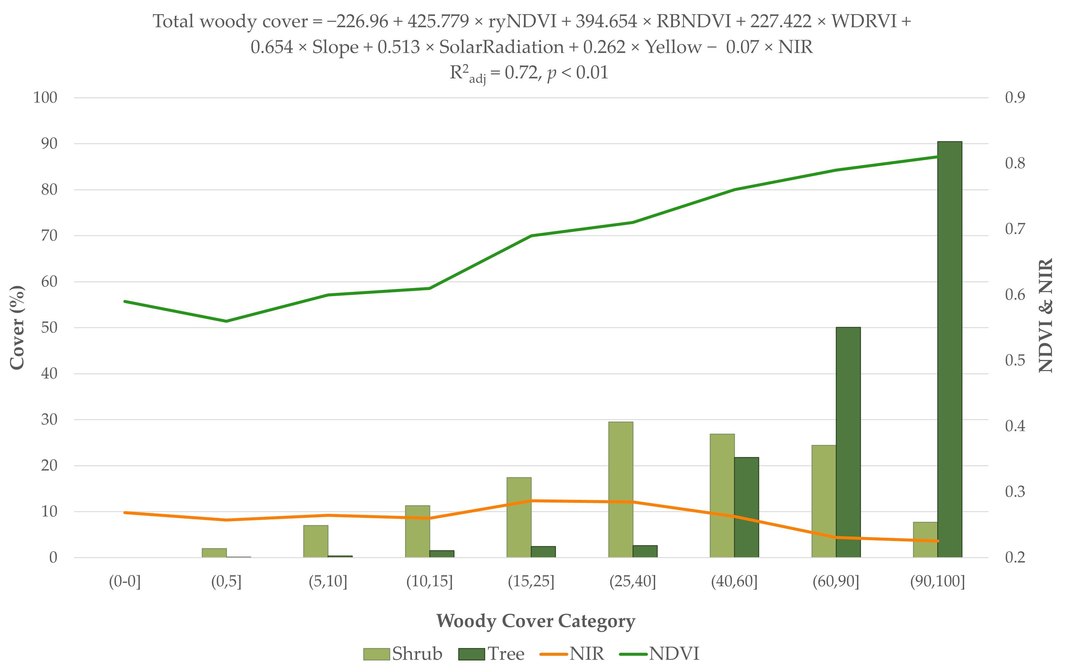
The best linear regression model of woody cover predicted by spectral and environmental data including the yellow and red-edge bands was as follows:

Total woody cover = −226.96 + 425.779 × ryNDVI + 394.654 × RBNDVI + 227.422 × WDRVI + 0.654 × Slope + 0.513 × SolarRadiation + 0.262 × Yellow − 0.07 × NIR (R²_adj = 0.72, p < 0.01)

(2)

The best model included the yellow band, which is not commonly included in satellite sensors; therefore, we developed a second model where the yellow band and associated vegetation indices were excluded. That model equation is as follows:

Total woody cover = −433.644 + 1356.912 × RBNDVI − 656.025 × ATSAVI + 0.512 × Slope + 0.264 × RED − 0.212 × GREEN I − 0.042 × NIR (R²_adj = 0.70, p < 0.01)

(3)

Finally, to generate a model compatible with the broadest range of sensors, we constructed a model including only the red band, NIR band, NDVI, and environmental variables. This model had lower r², demonstrating the value of the yellow band in woody cover estimation.

Total woody cover = −276.74 + 534.693 × NDVI + 0.191 × Red − 0.059 × NIR (R²_adj = 0.65, p < 0.01)

(4)

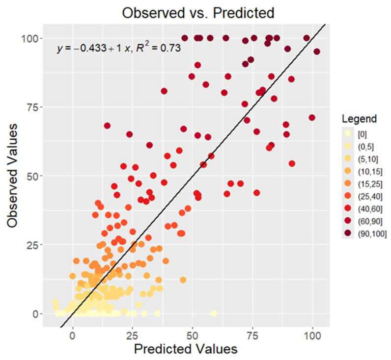
As seen in Figure 2, the primary developed model, using all bands and environmental data, is effective at predicting woody cover. There is some uncertainty, causing some degree of either over- or underestimation, but overall, the model functions well at a landscape level. A generalized least squares method might be more effective for future investigations in producing a model that functions well at a plot scale.

3.4. Mapping Woody Cover for the Study Area

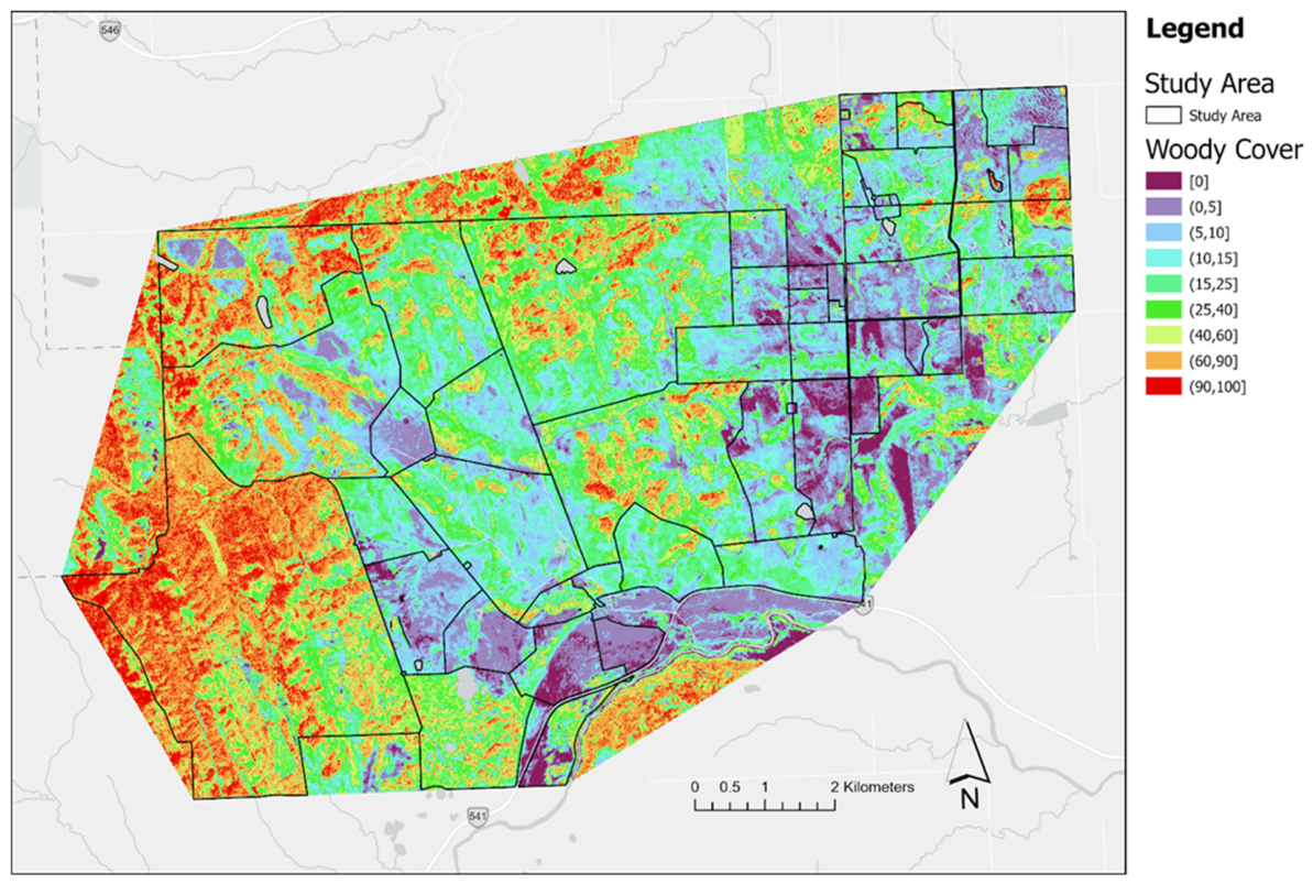
Using the best regression model, a map of the estimated woody cover area was produced. The model produced a continuous cover estimation that was then reclassified into the woody cover class groups used in the earlier investigation (Figure 3).

The cover area produced by the classification of the Planet Imagery was 103 km² (

Table 7. Values of woody cover distribution over eight woody cover categories.

Woody Cover	[0]	(0–5]	(5–10]	(10–15]	(15–25]	(25–40]	(40–60]	(60–90]	(90–100]
km2	3	11	13	11	16	13	12	17	7
% Area	3	11	13	11	15	13	12	17	6

). The areas of highest tree cover are dominated by hilly topography and slope and aspect features linked to increased tree cover. Places with more moderate woody plant cover tend to border existing areas of high cover, potentially relating to the expansion of woody cover, or lie along water features, relating to the higher-moisture preferences of some woody species. The lowest areas of woody cover are found around the flatter topography. A total of 5% of the area was predicted by the model to fall outside the 0–100% cover bounds; these values were truncated to 0 and 100.

4. Discussion

4.1. A Grassland Is a Complex Ecosystem

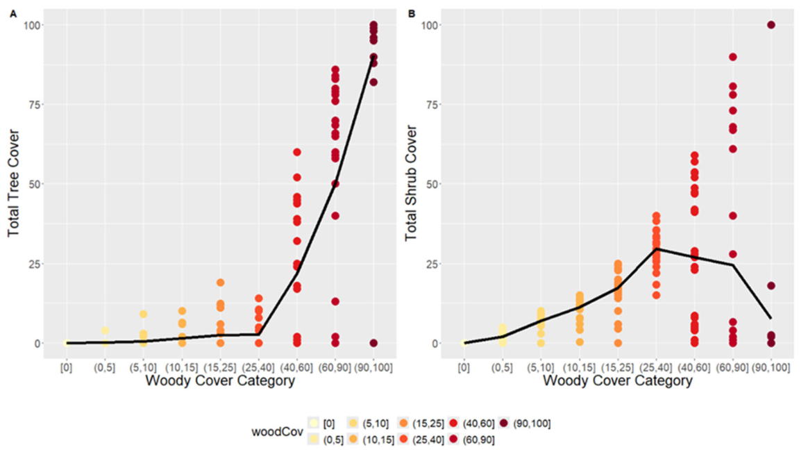
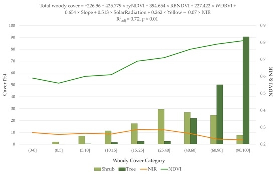
A healthy grassland ecosystem is composed of a mix of functional groups; the fescue grasslands in the study area are dominated by Festuca campestris and Carex spp. but always have a woody component [59]. The proportion of woody species will vary with long-term environmental trends, such as expansion with increased high intensity rainfall and dieback with drought [59,60]. Species composition is diverse, including short shrub species and tall tree species, with shorter, shrubby species dominating the middle woody cover range, while tree species dominate the higher-woody-cover categories (Figure 4). While woody species are a natural component of this ecosystem, detecting increases in woody plant cover above the historical norm is important. Here, we show that the two major woody functional groups, trees and shrubs, have differing environmental responses and spectral characteristics.

Environmental factors related to moisture availability were an important determinant of woody plant distribution in this montane landscape. White spruce had the strongest response, preferring northern aspects with lower incoming solar radiation, a pattern consistent with the species’ greater moisture requirements [61]. Similarly, the higher cover of white spruce and trembling aspen on lower slopes is likely due to higher-moisture preferences, leading to better growth on sites with higher water infiltration [24]. For shorter-statured shrub species such as Rosa sp., the drier mid-slope conditions are more favorable [24]. Willows had a strong positive response to increased TWI but did not respond to other environmental factors. This shows a preference for higher moisture that is being satisfied by different conditions than white spruce and aspen, possibly relating to a preference for riparian areas, or an additional temperature factor influencing white spruce. Altogether, this shows the expected complexity presented by a variety of woody plant species with unique environmental preferences. We can see some of the impact of this complexity in the modeling from the small R² values in Figure A2, Figure A3 and Figure A4. The natural heterogeneity of the community means each considered factor needs to account for more overall variability.

4.2. The Roles of Spectral and Spatial Properties of Imagery

Our results show the value of the yellow and red bands in predicting woody cover. Both the Red–Yellow Normalized Difference Vegetation Index (ryNDVI) and the base yellow band were important predictors in the best model. The second- and third-most impactful variables were the RBNDVI and WDRVI, which each make use of the red band. In the second-best model, the value of the red band and NIR becomes apparent. Three of the six significant variables in the second model contain information from the red band, and two of them make use of NIR.

The differences in phenology between grass cover and woody plant cover have previously been explored as a key factor in distinguishing the two cover types. Differing rates of greening in the spring and senescence in the fall have highlighted these times of year as ideal for differentiating the two cover types [36]. The yellow band allows for the detection of some of these phenological differences. At the time of data collection, ongoing drought stress may have contributed to the less deeply rooted grass cover or shorter-statured plants experiencing more stress-related yellowing than the woody cover on site, thus aiding in detection using these characteristics despite data collection not occurring in an optimal season [62].

The lack of separability between the low-cover categories of our results is similar to the findings of the study conducted by [30] and exemplifies the ongoing challenge of detecting woody plants at low cover values. The 3 m spatial resolution used here is much larger than individual shrubs, and species are closely intermingled [63,64]. These fine-scale occurrences are not readily detectable at the spatial resolution of current satellite platforms, supporting the need for investigation into alternate techniques with higher-spatial-resolution training data. Kattenborn et al. (2019) and Pu et al. (2025), for example, both used higher-spatial-resolution UAV imagery to successfully identify small patches of woody species [34,37]. Even at higher cover, however, the intermingled species in a typical grassland create spectral differences that make it hard to separate woody cover at higher stages as well. Short-wave infrared (SWIR) wavelengths are useful for woody plant encroachment detection [31,35,36]; however, to take advantage of the higher-spatial-resolution satellite imagery of Planet, we sacrificed access to the SWIR bands. A multi-spatial, multi-spectral, and multi-temporal approach may also be valuable as a tool for identifying woody species [30].

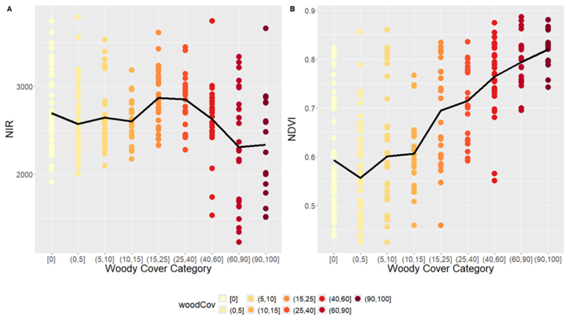
The spectral variables that were most valuable for separating woody cover categories were not the same as the variables important in the total woody cover estimation regression model. Investigating this discrepancy identified a non-linear NIR relationship with woody cover, showing much lower NIR reflectance above 40% woody cover, while increasing NDVI was closely correlated with increasing cover (Figure 5). This relationship is likely due to the differing physical structure of trees and shrubs [65]. This may provide a pathway to differentiating the two in the future. Sites with high woody cover are dominated by tall trees. Shadows and non-photosynthetic branches cause lower NIR reflectance. The same explanation can be applied to the slight dip in NDVI in the (0–5] category compared to 0% woody cover as grass cover is replaced by a small component of shrubs with woody stems. When the regression model was developed, variables were selected based on different levels of contribution to the woody cover estimation. Even though the NIR band did not present with high power to separate woody cover categories, it still provides information on detecting woody cover significantly at a lower level (e.g., coefficient of −0.07).

5. Conclusions

Woody plant encroachment is a complex phenomenon where multiple species with varying size, structure, and habitat requirements displace herbaceous functional groups in a grassland ecosystem. Here, we examine a site with complex topography and woody plant communities dominated by both shrubs and trees. Combining environmental variables and spectral data, we were able to estimate woody plant cover at an acceptable accuracy (r² = 0.73). We show that high spectral resolution is important for estimating woody cover. We also show the potential of the yellow spectral region as an asset in detecting WPE, as the yellow band and newly developed ryNDVI index both played a role in the best models. Finally, we show that differences in the relationships between NIR and NDVI and woody cover may provide a method to separate low shrub cover from tree cover. Some of the differences between shrub cover and tree cover that emerged in this investigation also highlight the value of considering tree and shrub cover as separate parts of the overall picture of WPE.

Investigating detailed categories of woody cover is imperative to detecting and managing the early stages of woody plant encroachment. In an attempt to map the temporal woody cover levels for detailed categories, we found that it was still a challenge to detect woody plant encroachment at an early stage (<15%). The developed models still provided a good estimate of woody cover trends in the study area, enabling management strategies to more effectively target key areas. In the future, further investigation into the use of high-resolution imagery and spectral trends at early stages will be vital for the effective monitoring of woody plant encroachment.

References

1. Scholtz, R.; Twidwell, D. The last continuous grasslands on Earth: Identification and conservation importance. Conserv. Sci. Pract. 2022, 4, e626. [Google Scholar] [CrossRef] [Scilit]
2. Friedman, S. Saving our Grasslands Why They Matter, Why We Are Losing Them, and How We Can Save Them; World Wildlife Fund Inc.: Washington, DC, USA, 2023; Available online: https://www.worldwildlife.org/publications/saving-our-grasslands-why-they-matter-why-we-are-losing-them-and-how-we-can-save-them/ (accessed on 4 February 2026).
3. Bardgett, R.D.; Bullock, J.M.; Lavorel, S.; Manning, P.; Schaffner, U.; Ostle, N.; Chomel, M.; Durigan, G.; Fry, E.L.; Johnson, D.; et al. Combatting global grassland degradation. Nat. Rev. Earth Environ. 2021, 2, 720–735. [Google Scholar] [CrossRef] [Scilit]
4. Li, J.; Ravi, S.; Wang, G.; Van Pelt, R.S.; Gill, T.E.; Sankey, J.B. Woody plant encroachment of grassland and the reversibility of shrub dominance: Erosion, fire, and feedback processes. Ecosphere 2022, 13, e3949. [Google Scholar] [CrossRef] [Scilit]
5. Palit, R.; DeKeyser, E.S. Impacts and Drivers of Smooth Brome (Bromus inermis Leyss.) Invasion in Native Ecosystems. Plants 2022, 11, 1340. [Google Scholar] [CrossRef] [Scilit] [PubMed]
6. Dettlaff, M.A.; Erbilgin, N.; Cahill, J.F. An invasive grass and litter impact tree encroachment into a native grassland. Appl. Veg. Sci. 2021, 24, e12618. [Google Scholar] [CrossRef] [Scilit]
7. Wilcox, B.P.; Fuhlendorf, S.D.; Walker, J.W.; Twidwell, D.; Ben Wu, X.; Goodman, L.E.; Treadwell, M.; Birt, A. Saving imperiled grassland biomes by recoupling fire and grazing: A case study from the Great Plains. Front. Ecol. Environ. 2021, 20, 179–186. [Google Scholar] [CrossRef] [Scilit]
8. Zhao, Y.; Liu, Z.; Wu, J. Grassland ecosystem services: A systematic review of research advances and future directions. Landsc. Ecol. 2020, 35, 793–814. [Google Scholar] [CrossRef] [Scilit]
9. Bork, E.W.; Burkinshaw, A.M. Cool-Season Floodplain Meadow Responses to Shrub Encroachment in Alberta. Rangel. Ecol. Manag. 2009, 62, 44–52. [Google Scholar] [CrossRef] [Scilit]
10. Twidwell, D.; Rogers, W.E.; Fuhlendorf, S.D.; Wonkka, C.L.; Engle, D.M.; Weir, J.R.; Kreuter, U.P.; Taylor, C.A. The rising Great Plains fire campaign: Citizens’ response to woody plant encroachment. Front. Ecol. Environ. 2013, 11, 64–71. [Google Scholar] [CrossRef] [Scilit]
11. Van Auken, O. Causes and consequences of woody plant encroachment into western North American grasslands. J. Environ. Manag. 2009, 90, 2931–2942. [Google Scholar] [CrossRef] [Scilit] [PubMed]
12. Statistics Canada. Cattle and Calves Statistics, Number of Farms Reporting and Average Number of Cattle and Calves per Farm. Table 32-10-0151-01. Available online: https://www150.statcan.gc.ca/t1/tbl1/en/tv.action?pid=3210015101 (accessed on 31 March 2026).
13. Archer, S.R.; Andersen, E.M.; Predick, K.I.; Schwinning, S.; Steidl, R.J.; Woods, S.R. Woody Plant Encroachment: Causes and Consequences. In Springer Series on Environmental Management Rangeland Systems Processes, Management and Challenges; Briske, D.D., Ed.; Springer: Durham, NC, USA, 2017. [Google Scholar] [CrossRef] [Scilit]
14. Soubry, I.; Guo, X. Invasive and native woody plant encroachment: Definitions and debates. J. Plant Sci. Phytopathol. 2022, 6, 084–086. [Google Scholar] [CrossRef] [Scilit]
15. Strand, E.K.; Blankenship, K.; Gucker, C.; Brunson, M.; MontBlanc, E. Changing fire regimes in the Great Basin USA. Ecosphere 2025, 16, e70203. [Google Scholar] [CrossRef] [Scilit]
16. Wilsey, B.J. The Biology of Grasslands, 1st ed; Oxford University Press: Oxford, UK, 2018. [Google Scholar]
17. Anderies, J.M.; Janssen, M.A.; Walker, B.H. Grazing Management, Resilience, and the Dynamics of a Fire-driven Rangeland System. Ecosystems 2002, 5, 23–44. [Google Scholar] [CrossRef] [Scilit]
18. Capozzelli, J.F.; Miller, J.R.; Debinski, D.M.; Schacht, W.H. Restoring the fire–grazing interaction promotes tree–grass coexistence by controlling woody encroachment. Ecosphere 2020, 11, e02993. [Google Scholar] [CrossRef] [Scilit]
19. Miller, J.E.D.; Damschen, E.I.; Ratajczak, Z.; Özdoğan, M. Holding the line: Three decades of prescribed fires halt but do not reverse woody encroachment in grasslands. Landsc. Ecol. 2017, 32, 2297–2310. [Google Scholar] [CrossRef] [Scilit]
20. O’cOnnor, R.C.; Taylor, J.H.; Nippert, J.B. Browsing and fire decreases dominance of a resprouting shrub in woody encroached grassland. Ecology 2019, 101, e02935. [Google Scholar] [CrossRef] [Scilit] [PubMed]
21. Gross, D.V.; Lamb, E.G. Strategies to reintroduce prescribed fire as a grassland management process on the Canadian prairies. Ecol. Solut. Évid. 2025, 6, e70035. [Google Scholar] [CrossRef] [Scilit]
22. Ding, J.; Eldridge, D. The success of woody plant removal depends on encroachment stage and plant traits. Nat. Plants 2022, 9, 58–67. [Google Scholar] [CrossRef] [Scilit]
23. Snell, R.S.; Peringer, A.; Frank, V.; Bugmann, H. Management-based mitigation of the impacts of climate-driven woody encroachment in high elevation pasture woodlands. J. Appl. Ecol. 2022, 59, 1925–1936. [Google Scholar] [CrossRef] [Scilit]
24. de Jonge, I.K.; Olff, H.; Mayemba, E.P.; Berger, S.J.; Veldhuis, M.P. Understanding woody plant encroachment: A plant functional trait approach. Ecol. Monogr. 2024, 94, e1618. [Google Scholar] [CrossRef] [Scilit]
25. Fogarty, D.T.; Roberts, C.P.; Uden, D.R.; Donovan, V.M.; Allen, C.R.; Naugle, D.E.; Jones, M.O.; Allred, B.W.; Twidwell, D. Woody Plant Encroachment and the Sustainability of Priority Conservation Areas. Sustainability 2020, 12, 8321. [Google Scholar] [CrossRef] [Scilit]
26. Pouliot, D.; Alavi, N.; Wilson, S.; Duffe, J.; Pasher, J.; Davidson, A.; Daneshfar, B.; Lindsay, E. Assessment of Landsat Based Deep-Learning Membership Analysis for Development of fromto Change Time Series in the Prairie Region of Canada from 1984 to 2018. Remote Sens. 2021, 13, 634. [Google Scholar] [CrossRef] [Scilit]
27. Badreldin, N.; Prieto, B.; Fisher, R. Mapping Grasslands in Mixed Grassland Ecoregion of Saskatchewan Using Big Remote Sensing Data and Machine Learning. Remote Sens. 2021, 13, 4972. [Google Scholar] [CrossRef] [Scilit]
28. Shafeian, E.; Fassnacht, F.E.; Latifi, H. Mapping fractional woody cover in an extensive semi-arid woodland area at different spatial grains with Sentinel-2 and very high-resolution data. Int. J. Appl. Earth Obs. Geoinform. 2021, 105, 102621. [Google Scholar] [CrossRef] [Scilit]
29. Sankey, T.T.; Leonard, J.M.; Moore, M.M. Unmanned Aerial Vehicle−Based Rangeland Monitoring: Examining a Century of Vegetation Changes. Rangel. Ecol. Manag. 2019, 72, 858–863. [Google Scholar] [CrossRef] [Scilit]
30. Soubry, I.; Doan, T.; Chu, T.; Guo, X. A Systematic Review on the Integration of Remote Sensing and GIS to Forest and Grassland Ecosystem Health Attributes, Indicators, and Measures. Remote Sens. 2021, 13, 3262. [Google Scholar] [CrossRef] [Scilit]
31. Collins, C.H.; Skirvin, S.; Kautz, M.; Winston, Z.; Curley, D.; Corrales, A.; Bishop, A.; Bishop, N.; Norton, C.; Ponce-Campos, G.; et al. Rangeland Brush Estimation Tool (RaBET): An Operational Remote Sensing-Based Application for Quantifying Woody Cover on Western Rangelands. Remote Sens. 2023, 15, 5102. [Google Scholar] [CrossRef] [Scilit]
32. Soubry, I.; Guo, X. Quantifying Woody Plant Encroachment in Grasslands: A Review on Remote Sensing Approaches. Can. J. Remote Sens. 2022, 48, 337–378. [Google Scholar] [CrossRef] [Scilit]
33. Olariu, H.G.; Malambo, L.; Popescu, S.C.; Virgil, C.; Wilcox, B.P. Woody Plant Encroachment: Evaluating Methodologies for Semiarid Woody Species Classification from Drone Images. Remote Sens. 2022, 14, 1665. [Google Scholar] [CrossRef] [Scilit]
34. Kattenborn, T.; Lopatin, J.; Förster, M.; Braun, A.C.; Fassnacht, F.E. UAV data as alternative to field sampling to map woody invasive species based on combined Sentinel-1 and Sentinel-2 data. Remote Sens. Environ. 2019, 227, 61–73. [Google Scholar] [CrossRef] [Scilit]
35. Marston, C.G.; Aplin, P.; Wilkinson, D.M.; Field, R.; O’regan, H.J. Scrubbing Up: Multi-Scale Investigation of Woody Encroachment in a Southern African Savannah. Remote Sens. 2017, 9, 419. [Google Scholar] [CrossRef] [Scilit]
36. Soubry, I.; Guo, X. Identification of the Optimal Season and Spectral Regions for Shrub Cover Estimation in Grasslands. Sensors 2021, 21, 3098. [Google Scholar] [CrossRef] [Scilit] [PubMed]
37. Pu, Y.; Lu, X.; Soubry, I.; Guo, X. Early detection of woody plant encroachment in Canadian prairies using UAV imagery and transformer-based deep learning. Ecol. Inform. 2025, 90, 103354. [Google Scholar] [CrossRef] [Scilit]
38. Alberta Parks. Natural Regions & Subregions of Alberta A Framework for Alberta’s Parks; Alberta Parks: Edmonton, AB, Canada, 2015; Available online: https://www.albertaparks.ca/media/6256258/natural-regions-subregions-of-alberta-a-framework-for-albertas-parks-booklet.pdf (accessed on 5 February 2026).
39. Alberta Parks. OH Ranch Heritage Rangeland Management Plan 2010; Alberta Parks: Edmonton, AB, Canada, 2010; Available online: https://open.alberta.ca/dataset/419a93cb-9790-43e8-b5a6-66b6850079bf/resource/1c8787bb-8380-4493-8dc5-602b52a38233/download/2010-ohranchmgmtplan.pdf (accessed on 5 February 2026).
40. Willoughby, M.G.; DeMaere, C.; Alexander, M.A.; Karpuk, E. Ecological Sites of the Foothills Parkland Subregion: First Approximation; Alberta Government: Edmonton, AB, Canada, 2020. Available online: https://open.alberta.ca/dataset/8f0b4ee6-5b4c-4d30-8679-1d236c88b1f3/resource/f68c66e3-fb85-4bfa-af3b-327c12c2fdf0/download/af-ecological-sites-of-foothills-parkland-subregion-first-approximation.pdf (accessed on 14 April 2026).
41. Planet Team. Planet Application Program Interface: In Space for Life on Earth. San Francisco, CA. 2025. Available online: https://api.planet.com (accessed on 5 February 2026).
42. Adams, B.W.; Elhert, R.; Moisey, D. Range Plant Communities and Range Health Assessment Guidelines for the Foothills Fescue Natural Subregion of Alberta. Second Approximation; Alberta Sustainable Resource Development, Public Lands & Forests Division, Rangeland Management Branch: Edmonton, AB, Canada, 2005; Available online: https://open.alberta.ca/dataset/93ff9e5a-4014-45c2-9f15-8b93d02e7bd1/resource/ad04f519-b96c-4645-8107-6f9060233238/download/2005-foothillsfescue-naturalsubregionguide.pdf (accessed on 5 February 2026).
43. Climate Indicators–Annual Precipitation|Alberta.ca. Available online: https://www.alberta.ca/climate-indicators-annual-precipitation (accessed on 5 February 2026).
44. Alberta Provincial 25 Metre Raster. Mar. 01, 2017, Alberta Environment and Parks, Government of Alberta, Edmonton, Alberta. Available online: http://www.altalis.com/products/terrain/dem.html (accessed on 8 February 2026).
45. Soubry, I.; Guo, X. Earth observation for Shrub Encroachment. EGUsphere 2024, 2024, 1–28. [Google Scholar] [CrossRef] [Scilit]
46. Bragg, T.B.; Hulbert, L.C. Woody Plant Invasion of Unburned Kansas Bluestem Prairie. J. Range Manag. 1976, 29, 19–24. [Google Scholar] [CrossRef] [Scilit]
47. Daubenmire, R.F. Canopy Coverage Method of Vegetation Analysis. Northwest Sci. 1959, 33, 43–64. [Google Scholar]
48. Beven, K.J.; Kirkby, M.J. A physically based, variable contributing area model of basin hydrology. Hydrol. Sci. J. 1979, 24, 43–69. [Google Scholar] [CrossRef] [Scilit]
49. Sørensen, R.; Zinko, U.; Seibert, J. On the calculation of the topographic wetness index: Evaluation of different methods based on field observations. Hydrol. Earth Syst. Sci. 2006, 10, 101–112. [Google Scholar] [CrossRef] [Scilit]
50. PlanetScope. Planet Documentation. Available online: https://docs.planet.com/data/imagery/planetscope/#band-order-and-sensor-frequency (accessed on 9 February 2026).
51. Wei, Y.; Lu, M.; Yu, Q.; Li, W.; Wang, C.; Tang, H.; Wu, W. The normalized difference yellow vegetation index (NDYVI): A new index for crop identification by using GaoFen-6 WFV data. Comput. Electron. Agric. 2024, 226, 109417. [Google Scholar] [CrossRef] [Scilit]
52. Sulik, J.J.; Long, D.S. Spectral considerations for modeling yield of canola. Remote Sens. Environ. 2016, 184, 161–174. [Google Scholar] [CrossRef] [Scilit]
53. Baret, F.; Guyot, G. Potentials and limits of vegetation indices for LAI and APAR assessment. Remote Sens. Environ. 1991, 35, 161–173. [Google Scholar] [CrossRef] [Scilit]
54. Wang, F.-M.; Huang, J.-F.; Tang, Y.-L.; Wang, X.-Z. New Vegetation Index and Its Application in Estimating Leaf Area Index of Rice. Rice Sci. 2007, 14, 195–203. [Google Scholar] [CrossRef] [Scilit]
55. Rondeaux, G.; Steven, M.; Baret, F. Optimization of soil-adjusted vegetation indices. Remote Sens. Environ. 1996, 55, 95–107. [Google Scholar] [CrossRef] [Scilit]
56. Rouse, J.W., Jr.; Haas, R.H.; Schell, J.A.; Deering, D.W. Monitoring vegetation systems in the Great Plains with ERTS. In Goddard Space Flight Center 3d ERTS-1 Symp.; NASA: Washington, DC, USA, 1974; Volume 1. [Google Scholar]
57. Gitelson, A.A. Wide Dynamic Range Vegetation Index for Remote Quantification of Biophysical Characteristics of Vegetation. J. Plant Physiol. 2004, 161, 165–173. [Google Scholar] [CrossRef] [Scilit]
58. R Core Team. R: A Language and Environment for Statistical Computing; R Foundation for Statistical Computing: Vienna, Austria; Available online: https://www.r-project.org/ (accessed on 7 November 2025).
59. Coupland, R.T. A Reconsideration of Grassland Classification in the Northern Great Plains of North America. J. Ecol. 1961, 49, 135–167. [Google Scholar] [CrossRef] [Scilit]
60. Kulmatiski, A.; Beard, K.H. Woody plant encroachment facilitated by increased precipitation intensity. Nat. Clim. Chang. 2013, 3, 833–837. [Google Scholar] [CrossRef] [Scilit]
61. Archibald, J.H.; Klappstein, G.D.; Corns, I.G.W. Field Guide to Ecosites of Southwestern Alberta; Northern Forestry Centre: Ottawa, ON, Canada, 1996. [Google Scholar]
62. Keen, R.M.; Helliker, B.R.; McCulloh, K.A.; Nippert, J.B. Save or spend? Diverging water-use strategies of grasses and encroaching clonal shrubs. J. Ecol. 2024, 112, 870–885. [Google Scholar] [CrossRef] [Scilit]
63. Attanayake, A.U. Incorporating Plant Community Structure in Species Distribution Modelling: A Species Co-Occurrence Based Composite Approach. Doctoral dissertation, University of Saskatchewan, Saskatoon, SK, Canada, 2020. Available online: https://harvest.usask.ca/items/1ce3f870-a8cb-4402-9262-603846a5a91a (accessed on 8 February 2026).
64. McNickle, G.G.; Lamb, E.G.; Lavender, M.; Cahill, J.F.; Schamp, B.S.; Siciliano, S.D.; Condit, R.; Hubbell, S.P.; Baltzer, J.L. Checkerboard score-area relationships reveal spatial scales of plant community structure. Oikos 2018, 127, 415–426. [Google Scholar] [CrossRef] [Scilit]
65. Xu, D.; Liu, Y.; Xu, W.; Guo, X. The Impact of NPV on the Spectral Parameters in the Yellow-Edge, Red-Edge and NIR Shoulder Wavelength Regions in Grasslands. Remote Sens. 2022, 14, 3031. [Google Scholar] [CrossRef] [Scilit]
Figure 1. Study area at the two ranches in southern Alberta, Canada, with 286 points sampled for ground reference in the summer of 2023 overlaid on the Planet Labs [41] Imagery © 2025 Planet Labs (true color composite) from July of the same year.
Remotesensing 18 01229 g001
Figure 2. Observed vs. predicted graph of the ground reference points compared to the values produced by the linear regression model (Equation (2)) at those points, with the identity line overlayed for reference. The mean square of the model was 239.01 and the standard deviation of the residuals was 15.46.
Remotesensing 18 01229 g002
Figure 3. Regression model map of woody cover area with the highest woody cover values in red and the lowest in purple.
Remotesensing 18 01229 g003
Figure 4. Line graph of average total tree (A) and total shrub cover (B) at each total woody cover category with sampling point data.
Remotesensing 18 01229 g004
Figure 5. Line graph of NIR (A) and NDVI (B) averages across woody cover categories with sample points.
Remotesensing 18 01229 g005