Article

Improved Quantification of Methane Point-Source Emissions from Hyperspectral Imagery Using a Spectrally Corrected Levenberg–Marquardt Matched Filter

1
State Key Laboratory of Remote Sensing and Digital Earth & Key Laboratory of Satellite Remote Sensing of Ministry of Ecology and Environment, Aerospace Information Research Institute, Chinese Academy of Sciences, Beijing 100101, China
2
University of Chinese Academy of Sciences, Beijing 100049, China
3
The Administrative Center for China’s Agenda 21, Beijing 100098, China
4
School of Emergency Management Science and Engineering, University of Chinese Academy of Sciences, Beijing 100049, China
*
Author to whom correspondence should be addressed.
Remote Sens. 2026, 18(8), 1195; https://doi.org/10.3390/rs18081195
Submission received: 27 February 2026 / Revised: 26 March 2026 / Accepted: 10 April 2026 / Published: 16 April 2026

Highlights

What are the main findings?
  • The developed Levenberg–Marquardt matched filter (LMMF) preserves the exponential absorption formulation, mitigating the systematic underestimation of the conventional MF under high-concentration methane conditions.
  • The proposed spectrally corrected LMMF (SC-LMMF) introduces a dynamic unit absorption spectrum (UAS) matching mechanism, reducing cross-scene systematic biases across multi-source hyperspectral satellite observations.
What are the implications of the main findings?
  • Restoring nonlinear absorption modeling and enforcing spectral consistency constraints represent an important pathway to improving the quantitative accuracy of MF-based methane point-source retrievals.
  • The proposed hierarchical retrieval framework demonstrates strong robustness and transferability, supporting refined methane emission monitoring and inventory verification using hyperspectral data.

Abstract

Spaceborne hyperspectral imaging spectrometers enable refined retrieval and quantification of methane point-source emissions. However, the conventional matched filter (MF) systematically underestimates methane enhancements under high-concentration conditions and remains sensitive to spectral inconsistencies across varying observation scenarios. To address these limitations, we improve MF-based retrieval from two aspects: the observation model and the unit absorption spectrum (UAS) representation. First, a Levenberg–Marquardt matched filter (LMMF) is developed by extending the MF framework to a nonlinear retrieval formulation while retaining its data-driven and background-statistics-based characteristics. Specifically, the exponential absorption term is preserved, and methane enhancement is iteratively solved in the nonlinear domain, enabling a more physically consistent retrieval without requiring precise external prior knowledge. Building upon this framework, a spectrally corrected LMMF (SC-LMMF) is further proposed by introducing a lookup-table-based dynamic UAS correction to account for variations in observation geometry, surface elevation, and atmospheric state. Comprehensive validation using idealized and noise-perturbed simulations, end-to-end simulations, and controlled-release experiments demonstrates that the LMMF mitigates high-concentration underestimation relative to the MF. The SC-LMMF further reduces cross-scene systematic biases, shifting retrievals toward a near 1:1 relationship. In controlled-release experiments, the SC-LMMF increased the coefficient of determination (R2) by approximately 50% while reducing the root mean square error (RMSE) and mean absolute error (MAE) by approximately 70% relative to the MF. Overall, the proposed framework enhances the robustness and quantitative consistency of methane point-source retrievals across multisource hyperspectral satellite observations.

1. Introduction

Methane (CH4) is the second most important greenhouse gas after carbon dioxide (CO2), with a 100-year global warming potential (GWP) approximately 27–30 times greater than that of CO2, making it a major contributor to climate forcing [1]. In recent years, global atmospheric methane concentrations have continued to rise, not only enhancing the greenhouse effect but also influencing atmospheric chemical processes such as oxidative capacity and ozone formation [2,3]. Therefore, in the context of global climate change mitigation, methane emission reduction is widely considered one of the most cost-effective near-term strategies [4,5]. Studies have shown that a substantial proportion of global methane emissions originates from anthropogenic activities, primarily from fossil fuel production, waste management, and agriculture [6,7,8,9]. These anthropogenic methane emissions often occur in the form of point sources, where relatively small facilities release large amounts of methane [10]. Accurate detection and quantification of methane point-source emissions are therefore essential for improving understanding of the carbon cycle, verifying emission inventories, evaluating mitigation policies, and supporting effective climate action [11,12].
Compared with ground-based and airborne observations, satellite remote sensing offers broader spatial coverage, higher revisit frequencies, and lower operational costs, emerging as a primary approach for monitoring greenhouse gas emissions [13,14,15,16]. At the global and regional scales, mapping missions represented by Sentinel-5P/TROPOMI have played an important role in large-scale methane anomaly identification and super-emitter detection owing to their wide swath coverage and rapid revisit capability [17,18]. However, due to their relatively coarse spatial resolution, such platforms are generally unable to attribute emissions precisely to individual facility-level point sources. With the increasing demand for precise localization and rapid response to methane point-source emissions, high-spatial-resolution imaging spectrometers have attracted growing attention. In recent years, multispectral imaging satellites, including Landsat-8/9, WorldView-3, and Sentinel-2A/2B [19,20,21], as well as hyperspectral imaging satellites such as the Gaofen-5/5A/5B, Ziyuan-1E/1F, PRISMA, EnMAP, EMIT, and Tanager-1 [22,23,24,25,26,27], have demonstrated significant progress in methane point-source detection, enabling identification and preliminary quantification of localized emission sources. Concurrently, a new generation of dedicated greenhouse gas monitoring satellites, such as GHGSat, MethaneSAT, XIGUANG-004, and Bikong-1, has either been deployed or is slated for launch [28,29,30,31]. By combining high spatial and spectral resolutions, these advanced missions further enhance the detection sensitivity and quantitative capabilities of spaceborne methane monitoring. Leveraging these platforms to exploit the distinctive methane absorption features in the shortwave infrared (SWIR) spectral region, numerous studies have successfully mapped and quantified anthropogenic methane emissions across key sectors, including oil and gas facilities, coal mines, and landfills [32,33,34,35].
Current satellite-based retrieval algorithms for methane point sources can be broadly categorized into physics-based and data-driven approaches. Physics-based methods—encompassing full-physics retrieval algorithms [36], CO2 proxy methods [29], WFM-DOAS [37], and IMAP-DOAS [38]—explicitly model radiative transfer processes to retrieve gas concentrations. In contrast, data-driven approaches are prominently represented by the matched filter (MF) algorithm [39,40,41], which estimates methane enhancements by exploiting the spectral contrast between target absorption features and background variability. Owing to its reduced dependence on precise a priori atmospheric information and its high computational efficiency, the MF has emerged as the most widely adopted algorithmic framework for methane point-source detection using imaging spectrometers. Building upon this framework, numerous studies have proposed methodological refinements to improve retrieval accuracy and robustness. For instance, Foote et al. [41] enhanced plume detection sensitivity by incorporating sparse priors and albedo correction. Roger et al. [42] extended the retrieval spectral range to introduce additional spectral information, thereby suppressing noise and artifacts. Furthermore, Li et al. [43] proposed the Sparse Spectral Reconstruction enhanced Matched Filter (SSRMF), which employs spectral matrix decomposition and low-rank reconstruction to better model background spectra. By introducing spatial continuity regularization into the cost function for methane enhancement estimation, this approach significantly improves plume coherence and retrieval performance under heterogeneous surface conditions.
Despite these methodological advancements, the systematic underestimation of methane enhancements by the conventional MF algorithm under high-concentration conditions remains a critical challenge. This underestimation generally stems from two primary sources. First, in constructing the observation model, the MF relies on a first-order linear approximation to describe methane absorption. For substantial methane enhancements, this linear assumption fails to accurately capture the nonlinear relationship between radiance and absorption, thereby introducing significant retrieval bias. Second, the conventional MF characterizes background radiative properties using image-wide statistical estimates without explicitly excluding plume-affected pixels. Consequently, the background mean and covariance matrix become contaminated by the target signal, further exacerbating the underestimation in high-concentration regions. To mitigate these limitations, several studies have proposed modifications to the MF framework. For instance, Schaum [44] replaced the conventional Gaussian model with a lognormal distribution, developing the Lognormal Matched Filter (LMF) to better characterize nonlinear absorption behavior. Kim et al. [45] proposed the Iterative Matched Filter (IMF), which iteratively updates the background mean and covariance matrix to mitigate contamination from high-concentration plume pixels. Building on these concepts, Pei et al. [46] combined both approaches into the Iterative Lognormal Matched Filter (ILMF) to simultaneously correct nonlinear absorption effects and background contamination. Furthermore, Liang et al. [47] introduced a piecewise regression strategy known as the Multi-Level Matched Filter (MLMF), which constructs concentration-dependent absorption spectra and background statistics across different enhancement ranges to improve retrieval stability for strong emissions. Although these approaches partially alleviate the underestimation problem at high concentrations, they primarily introduce nonlinear corrections through statistical modeling or empirical segmentation strategies. Crucially, they do not explicitly preserve the physical, exponential attenuation mechanism of gas absorption within the observation model itself.
Within the MF-based methane retrieval framework, the unit absorption spectrum (UAS) serves as the fundamental link connecting satellite-observed radiance to methane column concentration enhancements (ΔXCH4). The accuracy of the UAS directly governs the physical consistency and quantitative reliability of the retrieval results. However, previous studies have demonstrated that the UAS is intricately dependent on observation geometry, atmospheric states, surface elevation, and the sensor’s spectral response function. Consequently, applying a fixed or empirically approximated UAS across diverse observational scenarios introduces additional systematic biases, thereby degrading retrieval accuracy [48]. Therefore, developing a dynamic UAS representation scheme capable of adapting to complex and varying observational conditions has emerged as a critical methodological challenge. Overcoming this hurdle is essential for ensuring cross-scene consistency and improving the quantitative accuracy of methane point-source retrievals.
To address these critical limitations, this study proposes a Levenberg–Marquardt Matched Filter (LMMF) framework for hyperspectral methane point-source retrieval. Rather than departing from the conventional MF paradigm, the LMMF extends it to a nonlinear retrieval formulation while preserving its data-driven nature and its reliance on background statistics. By retaining the exponential absorption term and solving methane enhancement iteratively with Levenberg–Marquardt optimization, the LMMF explicitly accounts for nonlinear absorption and enables more physically consistent retrievals under strong-emission conditions without requiring precise external prior knowledge. Building upon this foundation, we further develop a Spectrally Corrected LMMF (SC-LMMF) to mitigate uncertainties associated with the UAS. This extension introduces a dynamic spectral correction mechanism that effectively reduces biases arising from varying observational and environmental conditions. The proposed methods are systematically evaluated against the conventional MF algorithm through a comprehensive suite of tests, including idealized simulations, noise-perturbed simulations, end-to-end simulations, and controlled-release experiments. The results demonstrate that the LMMF effectively mitigates the underestimation caused by linear approximations in the conventional MF, while the SC-LMMF further reduces systematic biases associated with spectral inconsistencies. Overall, the SC-LMMF framework achieves improved retrieval accuracy and robustness, providing a reliable methodological foundation for future coordinated, multi-satellite methane emission quantification.

2. Materials and Methods

2.1. Methane Retrieval and Quantification Methods

2.1.1. Retrieval Window Selection

Hyperspectral retrieval of methane primarily relies on the absorption features of surface-reflected solar radiation in the SWIR region. Methane exhibits two main absorption bands in this spectral range, located near 1650 nm and 2300 nm, with the absorption around 2300 nm being significantly stronger. Simultaneously, water vapor and carbon dioxide also exhibit pronounced absorption features in the SWIR region; therefore, their potential spectral interference must be carefully evaluated when selecting the retrieval window.
Figure 1 illustrates the atmospheric transmittance spectra of water vapor, carbon dioxide, and methane over the 1500–2600 nm range, simulated using the HITRAN database. Although water vapor and carbon dioxide absorptions partially overlap with methane features in certain localized intervals, this interference is confined to specific sub-windows rather than spanning the entire SWIR region. As demonstrated by Roger et al. [42], when water vapor and carbon dioxide enhancements are spatially homogeneous across the scene, their induced radiance variations are effectively incorporated into the scene-average background statistics. Consequently, their impact on matched-filter-based methane retrievals remains limited. However, when water vapor or carbon dioxide enhancements spatially overlap with a methane plume, these additional absorption structures can interfere with the target spectral identification, leading to an underestimation of the retrieved methane enhancement. The severity of this underestimation correlates with the enhancement level of the overlapping trace gas. Within a narrow retrieval window strictly around 2300 nm, carbon dioxide interference is relatively weak, though overlapping water vapor can already attenuate the retrieved values. If the retrieval window is unselectively expanded, both gases can cause more pronounced underestimations due to the inclusion of strong absorption bands that deviate from the target methane signature.
Conversely, Roger et al. [42] also noted that utilizing a broader near-infrared spectral window generally helps reduce retrieval artifacts and suppress background noise. To balance these competing factors, it is crucial to avoid spectral bands dominated by interfering trace gases when expanding the window; otherwise, the methane retrieval performance will degrade. Based on these considerations, and taking into account the available spectral range of the hyperspectral sensor, this study selects the 1500–2500 nm range as the primary working window. In practical implementation, local channels heavily contaminated by water vapor and carbon dioxide interference are strictly masked out. The three retrieval algorithms detailed in the following sections are all implemented within this optimized spectral subset.

2.1.2. Matched Filter

Methane exhibits characteristic absorption features; consequently, variations in its concentration induce corresponding changes in the radiance recorded by remote sensing instruments at specific absorption wavelengths. According to the Beer–Lambert law, the observed radiance in the presence of a methane enhancement can be expressed as:
L = L 0 e α s
where α denotes the methane concentration enhancement, s represents the methane absorption spectrum, L 0 is the background radiance in the absence of the methane enhancement, and L is the radiance observed in the presence of the enhancement. Because α s is typically small, Equation (1) is conventionally approximated using a first-order Taylor expansion, yielding the following linearized form:
L L 0 α s L 0
Let the methane UAS be denoted as s = s . The methane target spectrum can then be expressed as t = s L 0 , where both s and t are negative, reflecting the absorptive nature of methane. The linearized observation model can therefore be rewritten as:
L = L 0 + α t + n
where n represents the noise term.
Given the statistical properties of hyperspectral data, radiance in the SWIR region is commonly assumed to follow a multivariate normal distribution, i.e., L N L 0 + α t , C , where C denotes the covariance matrix. Considering that methane plume pixels typically occupy only a marginal fraction of the image, both L 0 and C can be estimated from the entire image. Based on the maximum likelihood criterion, the optimization objective function of the matched filter can be formulated as:
argmin α i i = 1 M ( L i μ α i t ) T C 1 L i μ α i t
where i denotes the pixel index, and L 0 is approximated by the mean background radiance μ .
Taking the derivative of the objective function with respect to the enhancement parameter and equating it to zero yields the closed-form solution. This solution corresponds to the concentration-path length enhancement estimated by the MF algorithm:
α i = ( L i μ ) T C 1 t t T C 1 t
Assuming that the enhanced methane is primarily confined within an effective atmospheric layer of approximately 8 km, the concentration-path length enhancement can be converted into the column concentration enhancement using an empirical scaling factor of 1/8000 m−1 [22,49]. It should be noted, however, that this fixed-layer assumption may introduce additional uncertainties under varying meteorological conditions.

2.1.3. Levenberg–Marquardt Matched Filter

The conventional matched filter tends to systematically underestimate methane enhancements under high-concentration conditions. This limitation primarily arises from two factors: contamination of background statistics by plume pixels and linearization errors introduced when approximating the exponential absorption process in the observation model. To explicitly account for the nonlinear absorption behavior of methane, the observation model is reformulated to retain its exponential form:
L = L 0 e α s + n
Accordingly, the optimization objective function is reformulated as:
a r g   min α i i = 1 M ( L i L 0 e α i s ) T C 1 L i L 0 e α i s
Because the resulting objective function is nonlinear, the Levenberg–Marquardt (LM) algorithm is employed for parameter estimation. It effectively combines the advantages of the Gauss–Newton method and gradient descent, ensuring stable convergence while maintaining computational efficiency for nonlinear optimization problems. The specific procedure is summarized as follows:
  • Initialization: The methane concentration enhancement α i 0 is initialized using the solution derived from the IMF. Furthermore, to mitigate contamination from plume pixels, the initial background mean radiance L 0 and covariance matrix C are re-estimated after excluding preliminarily identified enhancement pixels.
  • Residual construction: For each pixel, the residual function is defined as:
    r i α i = L i L 0 e α i s
  • Jacobian matrix construction: Taking the partial derivative of the residual function with respect to the enhancement parameter yields the Jacobian matrix:
    J i = 𝜕 r i 𝜕 α i = L 0 s e α i s
  • Iterative update: At each iteration, the enhancement parameter is updated by solving the following LM equation:
    J i T C 1 J i + λ I δ i = J i T C 1 r i
    α i ( k + 1 ) = α i ( k ) + δ i
    where k denotes the iteration index, λ is the damping factor that controls convergence stability of the LM algorithm, and δ i denotes the parameter increment at the current iteration.
  • Convergence criterion: The iteration is terminated when the relative decrease in the objective function falls below 10−6 or when the maximum number of iterations (e.g., 50) is reached.
Upon convergence, the final estimated parameter α corresponds to the concentration-path length enhancement retrieved by the LMMF algorithm. Consistent with Section 2.1.2, this value can be converted to the column concentration enhancement using the established empirical scaling factor.

2.1.4. Spectrally Corrected Levenberg–Marquardt Matched Filter

The UAS characterizes the methane absorption capacity per unit concentration and optical path length. It serves as a key physical parameter linking the observed radiance to the methane enhancement within the matched filter framework and its extensions. In the conventional MF and several of its variants, the UAS is typically assumed to be a fixed baseline spectrum. However, under actual satellite observation conditions, the UAS varies systematically with the observation geometry, surface elevation, and atmospheric state. Consequently, employing a fixed UAS can lead to mismatches between theoretical absorption features and actual observed spectra, thereby introducing region-dependent systematic biases into the retrieval results. Accordingly, even when the observation model is physically consistent (as in the LMMF), adaptive correction of key spectral parameters remains necessary. To further improve the physical consistency and cross-scene stability of the LMMF under complex observation conditions, this study integrates a radiative-transfer-based spectral correction mechanism, proposing the SC-LMMF. This method constructs a multi-parameter lookup table (LUT) for the UAS, enabling the dynamic updating of the absorption spectrum based on specific observational conditions, thereby mitigating systematic errors induced by environmental variability.
  • Sensitivity Analysis of the Unit Absorption Spectrum
The UAS in this study is generated using the MODerate Resolution Atmospheric TRANsmission (MODTRAN) model [50]. An enhanced gas profile is first constructed by setting the background atmospheric methane concentration to 1.9 ppm. Stepwise concentration increments (0, 0.125, 0.25, 0.5, and 1 ppm) are subsequently superimposed onto this background to simulate varying emission strengths. Because anthropogenic emission plumes are primarily confined to the near-surface layer, the concentration increment is assumed to be uniformly distributed from the surface up to an altitude of 500 m, with the background concentration remaining constant above this level [41]. Assuming an effective atmospheric path length of approximately 8 km, these increments correspond to concentration-path length enhancements of 0, 1000, 2000, 4000, and 8000 ppm·m. High-spectral-resolution radiances are then simulated under these varying methane enhancement conditions over the wavelength range of 1400–2600 nm, which comprehensively covers the major SWIR methane absorption bands. The MODTRAN simulations are conducted at a fine spectral resolution of 1 cm−1 and are subsequently convolved with the spectral response function (SRF) of the target sensor to generate synthetic radiances at the instrument’s native resolution. For each spectral band, a least-squares regression is performed between the concentration-path length enhancements and the natural logarithm of the simulated radiance. The fitted slope of this regression is defined as the unit absorption coefficient for that specific band, thereby constructing the UAS across the full spectral range.
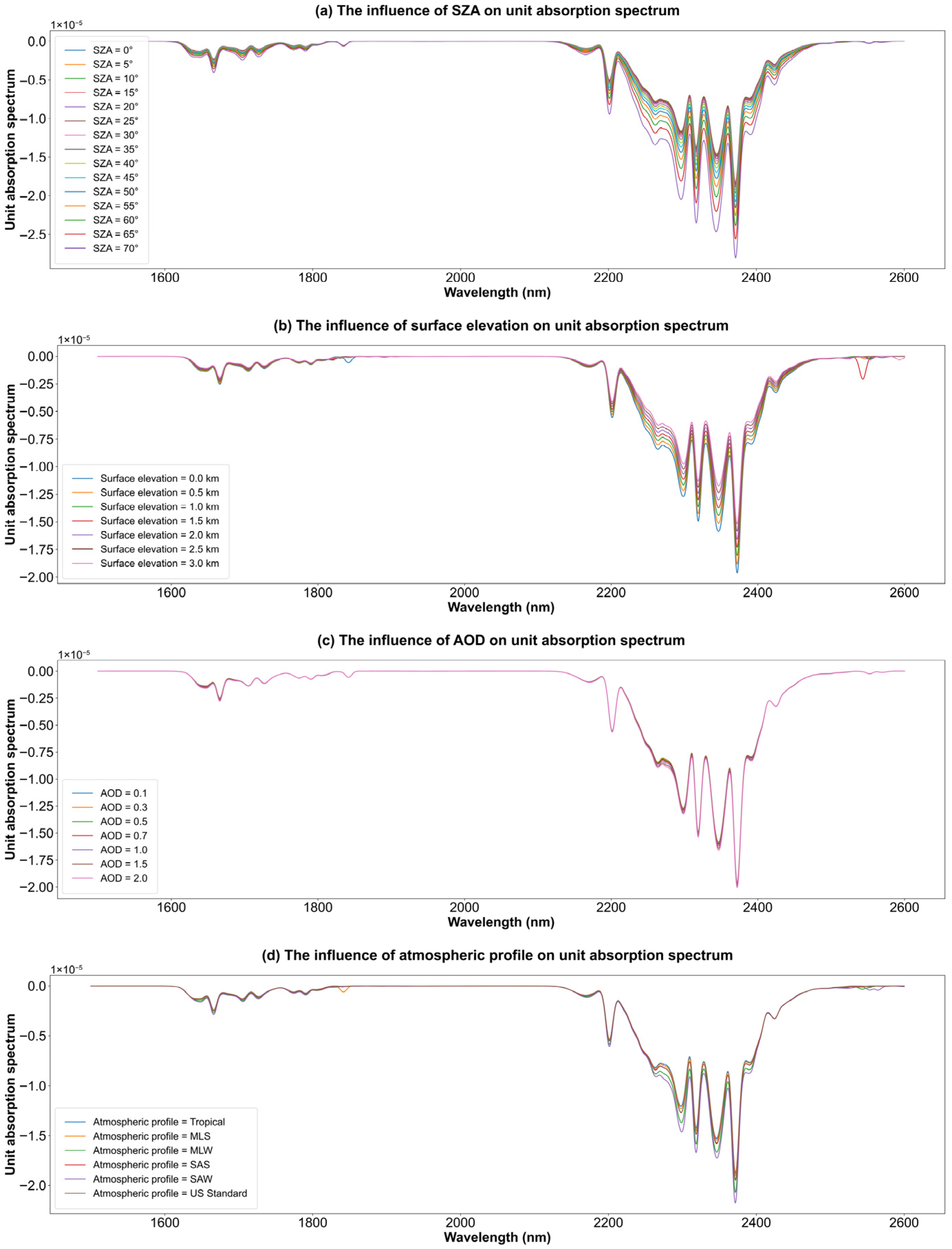
Because the UAS is inherently governed by the radiative transfer of gas absorption processes, its numerical characteristics are sensitive to key environmental factors, including the observation geometry, surface elevation, and atmospheric state. Given that the spaceborne sensor evaluated in this study primarily operates in a near-nadir viewing mode with a narrow field of view, variations in the satellite zenith angle (VZA) are minimal; therefore, the associated path-length perturbations are considered negligible. In contrast, the solar zenith angle (SZA) varies significantly with latitude, season, and time of overpass, making it the dominant geometric factor controlling the total optical path length. To quantitatively evaluate the influence of these environmental factors on the UAS, comprehensive sensitivity analyses are conducted by varying four primary parameters: SZA, surface elevation, aerosol optical depth (AOD), and atmospheric profile, employing a single-variable control approach.
Under the baseline simulation conditions, the SZA is set to 35°, surface elevation to 0 km, AOD to 0.3, and the atmospheric profile conforms to the U.S. Standard Atmosphere model. Each parameter is subsequently varied independently to isolate and assess its specific contribution to variations in the UAS. The evaluated parameter ranges and step sizes are summarized in Table 1 [48].
Figure 2 illustrates the response of the UAS to variations in SZA, surface elevation, AOD, and atmospheric profile. In terms of overall spectral morphology, variations in these parameters primarily induce nonlinear changes in the absorption depth within the strong methane absorption bands (centered near 1650 nm and 2300 nm), while the macroscopic shape of the spectrum remains highly stable. The baseline values in the non-absorbing channels exhibit minimal variation. Notably, while both strong and weak absorption bands exhibit consistent trend responses to environmental changes, the strong bands are substantially more sensitive to parameter variations. Among the investigated factors, geometric and topographic parameters—which directly govern the effective optical path length and the total gas column abundance—exert the dominant control. Specifically, as the SZA increases from 0° to 70°, the effective atmospheric optical path length lengthens considerably, resulting in deeper absorption features within the characteristic bands. Conversely, as the surface elevation increases from 0 km to 3.0 km, the effective vertical thickness of the atmospheric column decreases. This reduces the total number of methane molecules along the optical path, thereby leading to attenuated absorption features. Compared with these geometric and topographic effects, atmospheric state parameters exert a secondary influence. Increasing the AOD slightly enhances the absorption depth due to increased multiple scattering effects, although the overall magnitude of this perturbation remains limited. Furthermore, variations in the atmospheric profile primarily modify the gas absorption cross-sections by altering the vertical temperature and humidity distributions; consequently, the absorption strength is generally enhanced under cold, high-latitude conditions and weakened under tropical conditions.
2.
Look-Up Table Construction and Dynamic Matching Retrieval Model
Based on the sensitivity analysis, a LUT of the UAS was constructed. The LUT indexing dimensions include the SZA, surface elevation, AOD, and atmospheric profile. According to the sensitivity ranking of these factors, the SZA and surface elevation—identified as the dominant controlling parameters—were prioritized in the LUT construction. The atmospheric profile type was incorporated as a secondary indexing dimension. In contrast, because the AOD exerts a comparatively weaker perturbation on the absorption spectrum, it was treated with moderate simplification in the LUT design to optimize the balance between physical fidelity and parameter space complexity. During the SC-LMMF retrieval process, the nonlinear absorption observation model of the LMMF remains structurally unchanged; however, the fixed baseline absorption spectrum is replaced by a dynamically matched, LUT-derived UAS. The corresponding observation model can therefore be expressed as:
L = L 0 e α s c o n d + n
where s c o n d denotes the dynamically matched UAS retrieved from the LUT according to the prevailing observation conditions for each specific pixel. Through this strategy, the SC-LMMF preserves the advantages of nonlinear absorption modeling while further reducing the region-dependent systematic biases induced by UAS uncertainties. As a result, the proposed method demonstrates improved retrieval stability and cross-scene physical consistency under complex observational scenarios.

2.1.5. Plume Detection and Emission Quantification

Following the retrieval of the ΔXCH4, plume detection is subsequently performed. The primary objective of this stage is to identify statistically significant and spatially coherent emission signals within the retrieval results. First, a statistical analysis is conducted on the methane enhancements derived from the matched filter. A statistical threshold, typically set to one standard deviation above the background mean, is selected to initially identify pixels exhibiting anomalous enhancements. On this basis, a spatial contiguity constraint is introduced to retain spatially aggregated clusters while removing isolated noise pixels, thereby ensuring the physical coherence of the detected plume structures.
In practical applications, plume identification is further constrained by meteorological conditions and surface information. High-resolution optical imagery and the spatial distribution of known emission facilities are utilized to verify whether potential sources—such as oil and gas infrastructure, coal mines, and landfills—are located upwind or directly beneath the detected enhancement regions. A region is confirmed as a valid methane plume only when both meteorological consistency and source plausibility are satisfied.
After plume delineation, methane emission rates are quantified using the Integrated Mass Enhancement (IME) method. The ΔXCH4 of all pixels within the identified plume mask are first integrated and subsequently converted into a total mass enhancement using a unit conversion factor. The IME is calculated as:
IME = k i = 1 n p α i
where n p denotes the total number of valid plume pixels, α i represents the retrieved column concentration enhancement of the i-th pixel, and k is the unit conversion factor (kg/ppb), defined as:
k = M CH 4 R 2 H V mol × 10 9
where M CH 4 is the molar mass of methane (0.01604 kg / mol ), V mol is the molar volume of an ideal gas under standard conditions (22.4 × 10⁻³ m 3 / mol ), R denotes the pixel area determined by the spatial resolution of the sensor, H represents the effective atmospheric layer height (consistent with the 8 km assumption established in Section 2.1.1), and 10 9 is the ppb concentration conversion factor. The emission rate Q ( kg / h ) is then derived from the total plume mass as:
Q = U eff IME L
where L denotes the plume length scale and U eff represents the effective wind speed. The uncertainty of the emission rate Q is estimated following the error propagation framework proposed by Cusworth et al. [8].

2.2. Controlled-Release Experiment Data

To evaluate the accuracy and applicability of the proposed retrieval algorithms under real-world emission conditions, this study utilizes data from a controlled methane release campaign conducted by Stanford University in 2022 [51,52]. This campaign simulated diverse emission scenarios under rigorously controlled conditions, accompanied by precise in situ measurements, thereby providing a benchmark for the quantitative evaluation of retrieval performance. Specifically, the ground-truth reference data included metered methane emission rates and near-surface wind speed and direction measurements.
Concurrent with these controlled releases, hyperspectral radiance data were acquired by multiple satellite sensors, serving as the basis for concentration retrieval and plume identification. By comparing the satellite-derived emission rates against the metered ground-truth release rates, the quantitative performance and error characteristics of the different retrieval algorithms can be systematically assessed under realistic observational conditions. This integrated validation framework—combining ground-based reference data with multi-source satellite observations—provides important support for the rigorous validation and refinement of methane quantification methods.
In this study, one representative scene from each of four spaceborne hyperspectral satellites—GF5B, ZY1F, PRISMA, and EnMAP—was selected for the retrieval experiments. The corresponding sensor specifications and scene acquisition details are summarized in Table 2.

2.3. Simulation Data Generation

2.3.1. Methane Plume Simulation Using WRF-LES

To simulate the transport and dispersion of near-surface methane point-source emissions within the atmospheric boundary layer, a high-resolution Large Eddy Simulation (LES) model based on the Weather Research and Forecasting (WRF) system was employed to construct an idealized methane plume scenario. The WRF-LES framework is capable of resolving turbulent structures within the convective boundary layer and is particularly suitable for simulating plume evolution under non-steady atmospheric conditions [53].
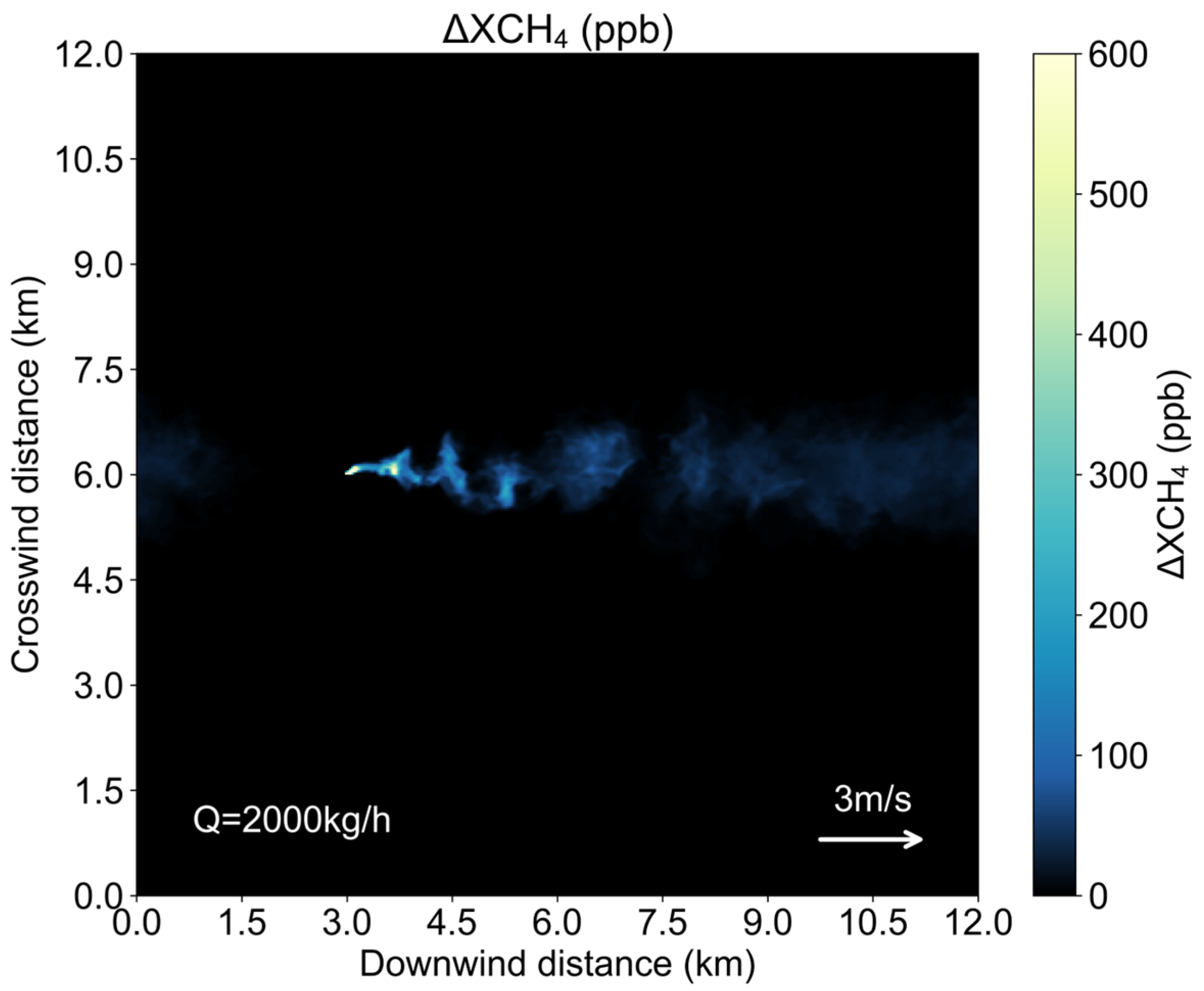
The simulation assumes clear-sky, cloud-free, and flat terrain boundary conditions. The horizontal spatial resolution is set to 30 m × 30 m, with a vertical resolution of 30 m. The simulation domain consists of 400 × 400 grid cells, corresponding to a total coverage area of 12 km × 12 km. The initial meteorological conditions follow the parameter settings established by Varon et al. [54]: the boundary layer height is set to 1000 m, the initial temperature within the mixed layer is uniformly 300 K, and the background wind speed is 3 m·s−1. Under these configurations, methane emissions from a continuous point source are introduced into the model utilizing the built-in passive tracer module of the WRF system. Methane is treated as a passive tracer, and its dispersion behavior within the highly resolved turbulent flow field realistically represents the spatial evolution of the emission plume. The total simulation duration is set to 1 h to capture the plume formation and its short-term transport dynamics. The detailed simulation parameters are summarized in Table 3.
The methane emission rate of the point source is initially set to 2000 kg·h−1. The simulated three-dimensional mass concentration field is then vertically integrated to obtain ΔXCH4. Figure 3 presents the instantaneous spatial structure of the plume under the configured scenario. This highly resolved synthetic dataset serves as a crucial input for the subsequent MODTRAN radiative transfer simulations and provides an idealized and controlled benchmark for evaluating the quantitative retrieval performance of the proposed algorithms.

2.3.2. Three Simulation Experiments

To systematically compare the retrieval performance of the MF, LMMF and SC-LMMF under varying environmental conditions, three distinct simulation experiments were designed in this study. The configuration details of these simulations are summarized in Table 4.
For all simulations, the background atmospheric methane column concentration was set to 1900 ppb. The top-of-atmosphere (TOA) radiances were simulated using the MODTRAN model. The baseline simulation parameters follow the configuration described in Section 2.1.3.
  • Idealized simulation
The first simulation represents idealized observational conditions. The TOA radiance is generated without considering surface reflectance effects or instrument noise and is utilized solely to evaluate the theoretical baseline performance of the retrieval algorithms. The ΔXCH4 is uniformly sampled from 0 to 1400 ppb at 40 ppb intervals, yielding 36 discrete samples that are subsequently superimposed onto the background methane profile.
2.
Noise-perturbed simulation
In the second simulation, a more realistic yet rigorously controlled environment is constructed based on the methane concentration field generated by the WRF-LES model. A mixed soil–vegetation surface reflectance is adopted, and 1% Gaussian noise is injected to simulate instrument measurement errors. This configuration deliberately introduces select real-world complexities while maintaining overall controllability, allowing for the robust evaluation of algorithm stability under more challenging conditions.
3.
End-to-end simulation
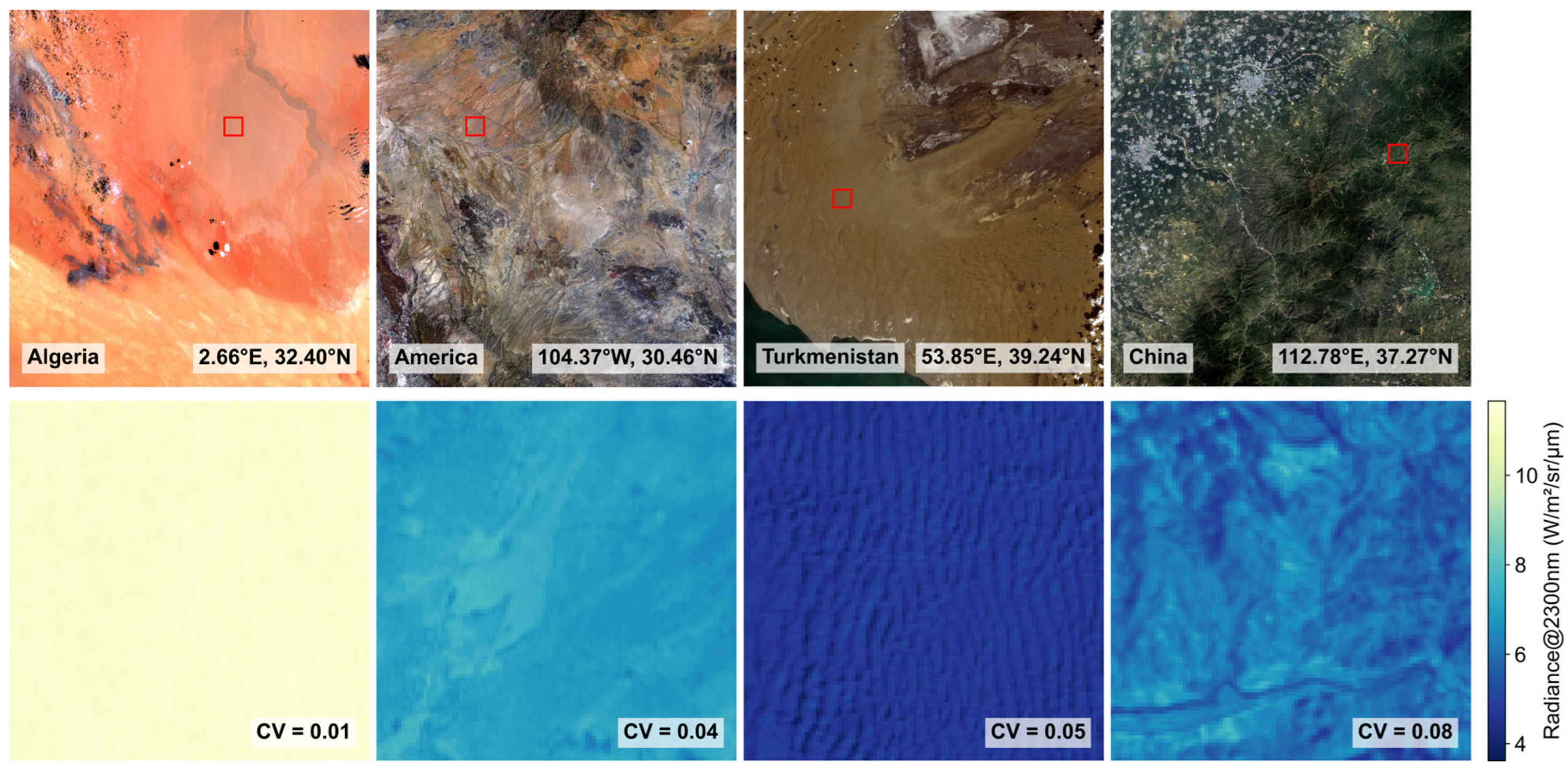
To further improve realism, the WRF-LES-simulated ΔXCH4 field is embedded into real observations from the GF5B/AHSI (Advanced Hyperspectral Imager) to generate synthetic plume-containing scenes. The specific procedure is executed as follows: First, MODTRAN is employed to simulate the high-resolution methane transmittance spectra based on the WRF-LES-simulated ΔXCH4 field. Second, these simulated spectra are convolved with the SRF of the AHSI sensor. Finally, the convolved transmittance spectra are multiplied by the original AHSI TOA radiances to generate synthetic observations containing realistic methane plume signals. This forward-modeling approach preserves the real spectral structure and spatial heterogeneity of the background surface, while incorporating the actual instrument response and complex noise characteristics of the AHSI sensor, thereby providing a more realistic test of algorithmic performance. Four GF5B/AHSI image subsets with diverse surface characteristics were carefully selected from representative methane emission hotspot regions located in Algeria, the United States, Turkmenistan, and China. These selected datasets are illustrated in Figure 4.

3. Results

3.1. Results of the Idealized Simulation

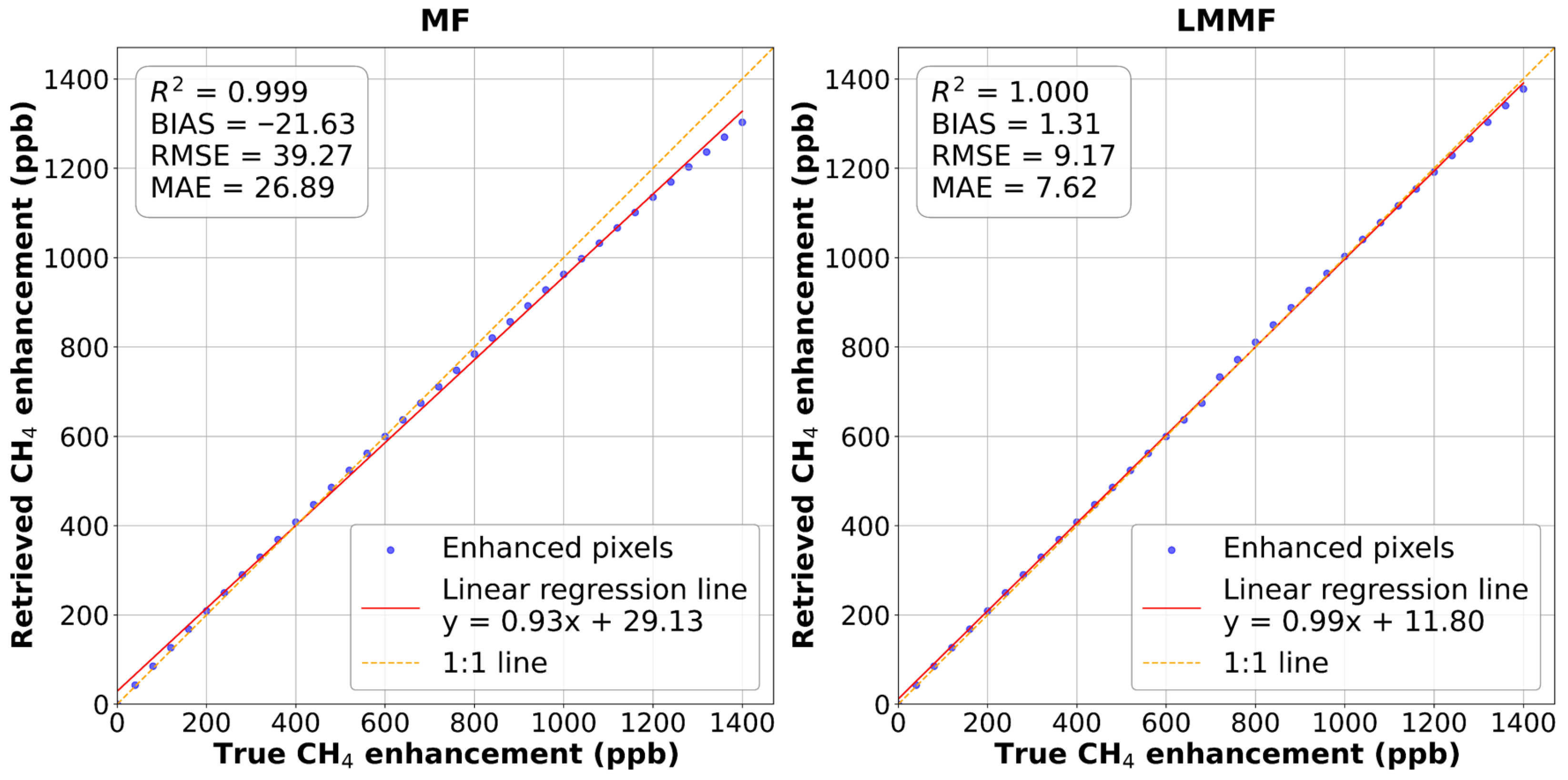
Figure 5 presents a quantitative comparison of the ΔXCH4 retrieved by the MF and LMMF algorithms using synthetic TOA radiance under idealized observation conditions.
Under noise-free conditions, both algorithms exhibit strong linear consistency between retrieved and true methane enhancements. For the conventional MF algorithm, although the coefficient of determination (R2) approaches 1.0—indicating a strong correlation—the regression slope is approximately 0.93, revealing systematic underestimation. This bias becomes increasingly evident at higher methane enhancement levels, where deviations from the 1:1 reference line are more pronounced. Correspondingly, the higher BIAS, root mean square error (RMSE) and mean absolute error (MAE) values reflect the limitation of MF in achieving accurate absolute quantification under elevated concentration conditions.
In contrast, the LMMF algorithm produces a regression slope close to unity while maintaining a similarly high R2. All absolute error metrics (BIAS, RMSE, and MAE) are reduced relative to those of MF. These results indicate that LMMF improves quantitative consistency across the full dynamic range of methane enhancements. By preserving the nonlinear exponential absorption term in the observation model, LMMF effectively alleviates the high-concentration underestimation inherent to the linearized MF formulation.

3.2. Results of the Noise-Perturbed Simulation

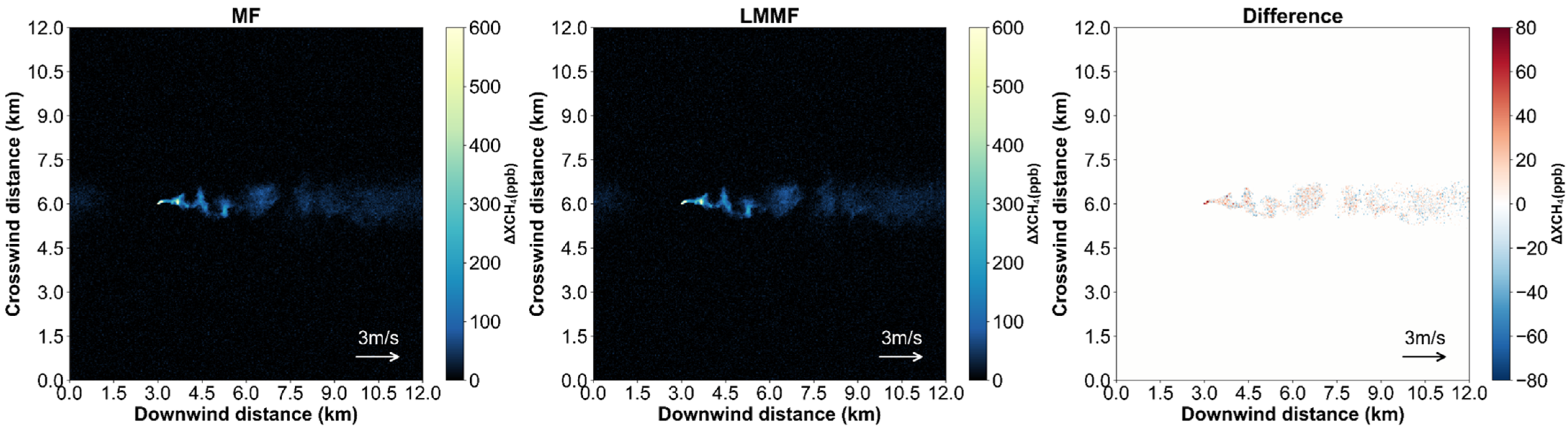
Using synthetic radiance data generated under the noise-perturbed scenario, ΔXCH4 were retrieved with both MF and LMMF. Figure 6 shows the spatial distributions of the retrieved plumes. From a spatial perspective, both algorithms successfully capture the plume morphology aligned with the prevailing wind direction, indicating reliable detection capability under noise contamination. The difference map indicates that LMMF generally produces slightly higher retrieved values than MF within the plume region.
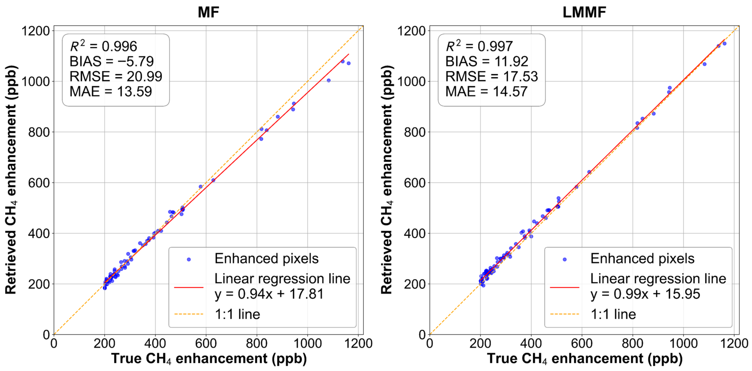
Figure 7 provides the quantitative comparison between retrieved and true ΔXCH4. To focus on the emission core and better assess high-concentration performance, pixels with true ΔXCH4 below 200 ppb were excluded from the scatter analysis. Both algorithms maintain strong linear correlations, with R2 values of 0.996 for MF and 0.997 for LMMF.
Despite the comparable correlations, notable differences appear in the regression parameters. The MF algorithm continues to exhibit systematic underestimation, characterized by a slope of 0.94 and an intercept of 17.81 ppb. In contrast, LMMF yields a slope of 0.99 and an intercept of 15.95 ppb, approaching the ideal 1:1 relationship. These findings indicate that the LMMF effectively mitigates the systematic negative bias observed in the MF method, particularly for high-enhancement pixels.
In terms of the absolute error metrics, the RMSE of the LMMF is substantially reduced compared to that of the MF, further supporting its improved quantitative accuracy and stability under realistic, noise-perturbed observational conditions.
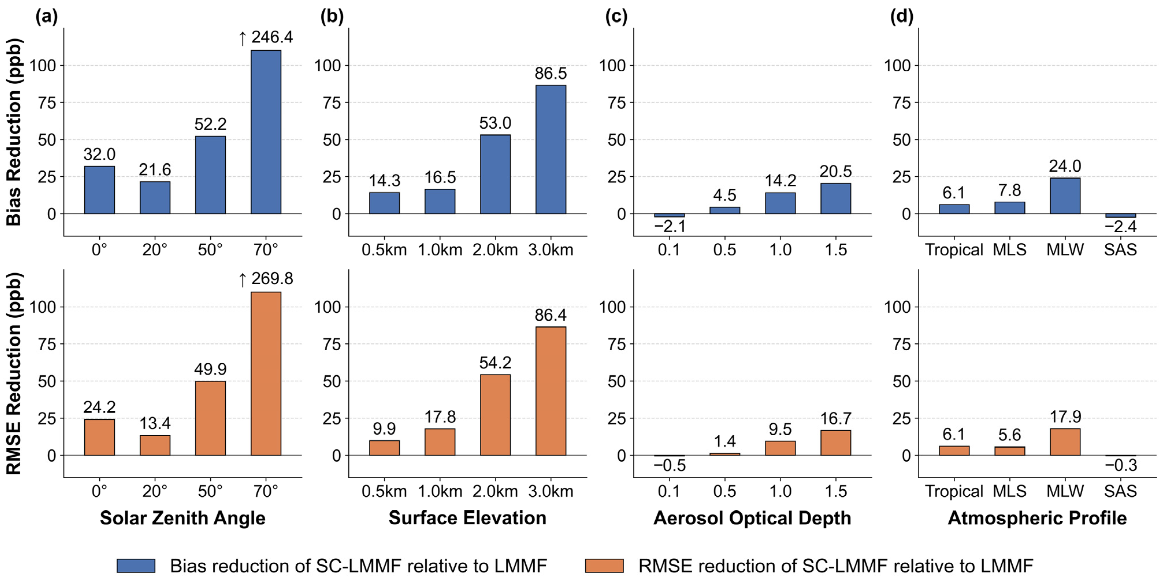
Figure 8 summarizes the improvements in error metrics achieved by the SC-LMMF driven by the dynamically accurate UAS relative to the LMMF driven by the baseline UAS under different observation conditions. Overall, the SC-LMMF yields positive bias reduction and RMSE reduction in most scenarios, indicating that it effectively alleviates systematic bias without introducing additional random errors. The improvement remains consistent across varying observation geometries, surface elevations, and atmospheric states, suggesting enhanced cross-scene retrieval consistency.
A more detailed comparison shows that the improvement of the SC-LMMF becomes more pronounced under large solar zenith angles and high surface elevations. This pattern indicates that when the solar geometry and surface elevation deviate substantially from the baseline configuration, the accurate physical representation of the UAS becomes increasingly important for retrieval performance.
It should also be noted that under observation conditions close to the baseline settings—such as moderate SZAs, low surface elevations, low to moderate AODs, and standard atmospheric profiles—the LMMF driven by the baseline UAS still achieves high retrieval accuracy. In these scenarios, the UAS remains relatively stable and closely aligned with the actual observation conditions, reducing the need for additional spectral correction.
In summary, the SC-LMMF can consistently improve the retrieval accuracy of methane enhancements under complex observational conditions and significantly reduce systematic bias. By contrast, when the observational conditions are close to the baseline scenario, the conventional LMMF is sufficient for quantitative retrieval, highlighting the differentiated applicability of the two methods across different application scenarios.

3.3. Results of the End-to-End Simulation

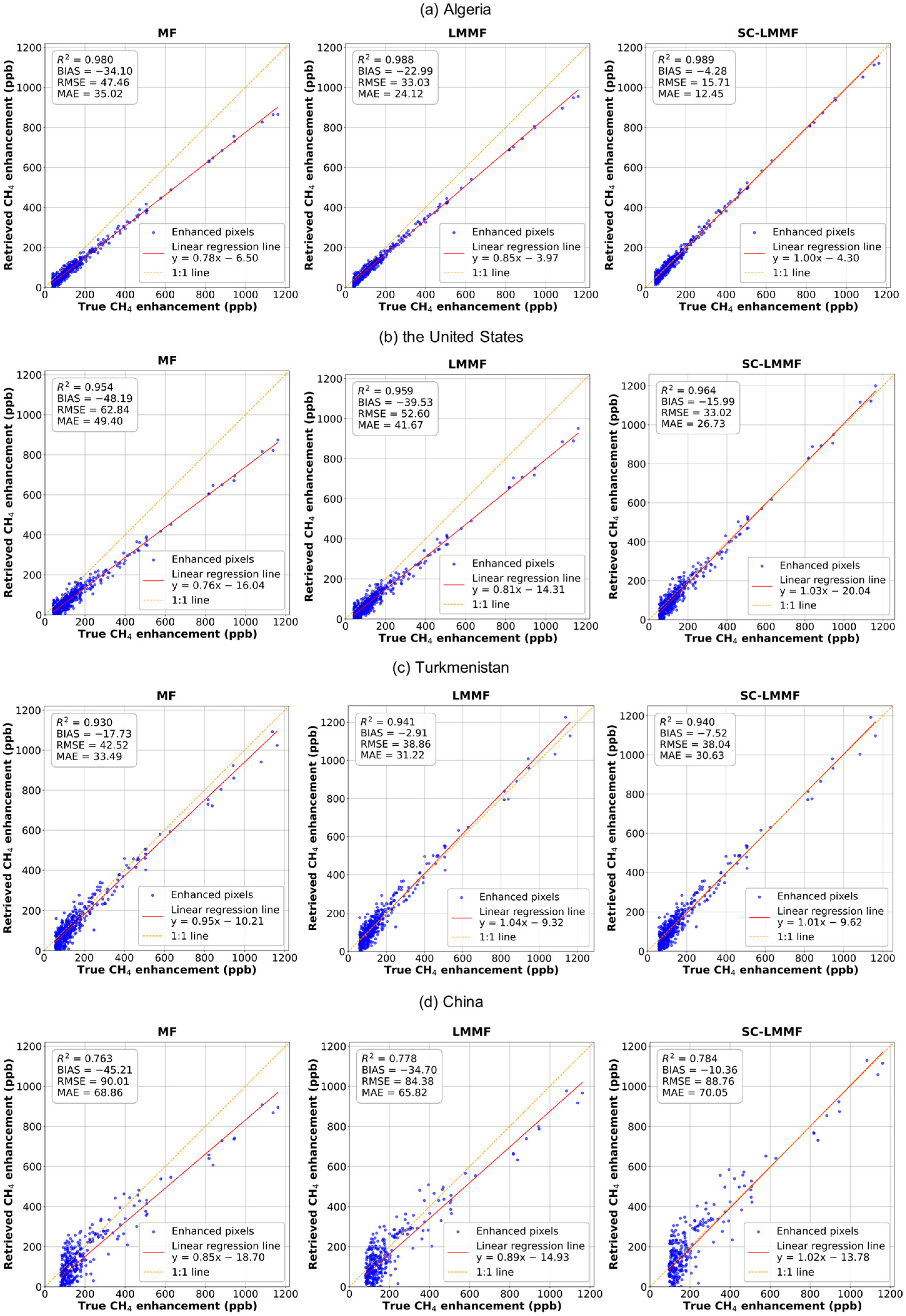
Figure 9 presents the retrieval results of the ΔXCH4 over four representative hotspot regions located in Algeria, the United States, Turkmenistan, and China. The scatter distributions and corresponding statistical metrics for the MF, LMMF, and SC-LMMF are shown for each region. Overall, the conventional MF consistently exhibits systematic underestimation across all study areas. The LMMF partially mitigates this issue, while the SC-LMMF demonstrates improved consistency and stability, indicating progressive improvements in retrieval accuracy among the three methods.
In regions characterized by relatively homogeneous surface conditions, such as Algeria and the United States, the improvements are particularly distinct. In Algeria, the MF yields a regression slope of 0.78 with a relatively high RMSE, indicating clear underestimation. The LMMF increases the slope to 0.85 but does not fully eliminate the bias. In contrast, the SC-LMMF corrects the slope to 1.00 and substantially reduces the RMSE, demonstrating improved performance in both magnitude recovery and linear consistency. A similar trend is observed in the United States, where the slope increases from 0.76 (MF) to 1.03 (SC-LMMF), accompanied by a marked reduction in the error metrics, indicating the stable applicability of the improved algorithm.
In regions with more complex surface structures and higher background variability, the SC-LMMF maintains improved physical consistency. In China, the MF and LMMF produce slopes of 0.85 and 0.89, respectively, both indicating underestimation. The SC-LMMF adjusts the slope to 1.02, effectively reducing the systematic bias. Although the RMSE increases slightly compared with the LMMF, this indicates that under high-noise conditions, the spectral correction mainly improves the systematic bias of the retrieval, whereas the random error remains constrained by observational noise. In Turkmenistan, where the actual UAS exhibits stronger absorption features than the baseline UAS, the LMMF slightly overcorrects the MF underestimation (slope = 1.04). The SC-LMMF effectively constrains this effect, stabilizing the slope at 1.01 and further reducing the RMSE, indicating that it remains robust under different spectral absorption characteristics.
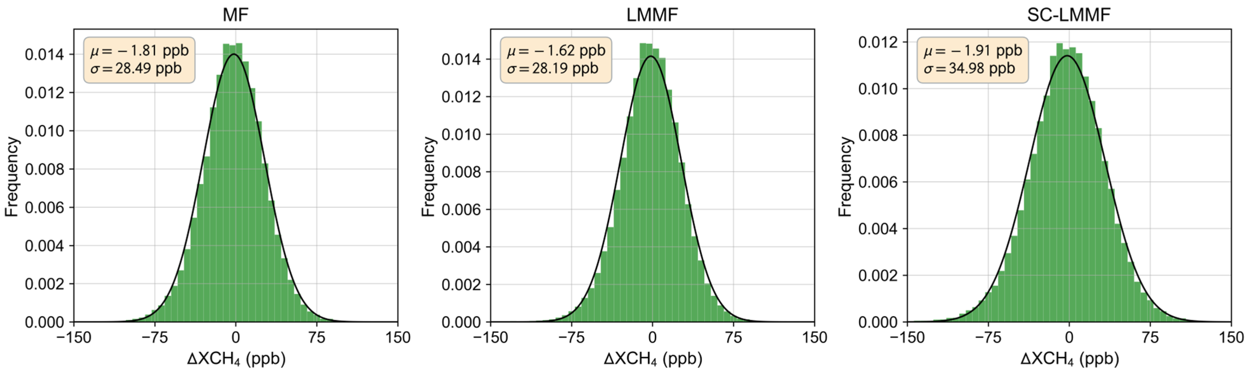
Figure 10 presents the histograms of ΔXCH4 for non-emission pixels in the United States region. These histograms are used to characterize the retrieval errors of the three methods under non-emission conditions and to further illustrate the detection-limit characteristics. The mean values of the three methods are all close to zero, and their standard deviations are also generally similar, indicating that none of the three methods introduces an obvious overall offset under non-emission conditions and that their retrieval precision remains at a comparable level. Since the detectability of weak plumes mainly depends on whether plume enhancements can be significantly distinguished from background noise, the standard deviation can be used as an approximate measure of retrieval precision and can further constrain the range of the minimum detectable emission rate. From this perspective, the detection limit of LMMF is slightly improved relative to that of MF, whereas the improvement introduced by SC-LMMF is not mainly reflected in a further reduction in the detection limit, but rather in the correction of high-concentration underestimation when the plume signal is sufficiently strong.
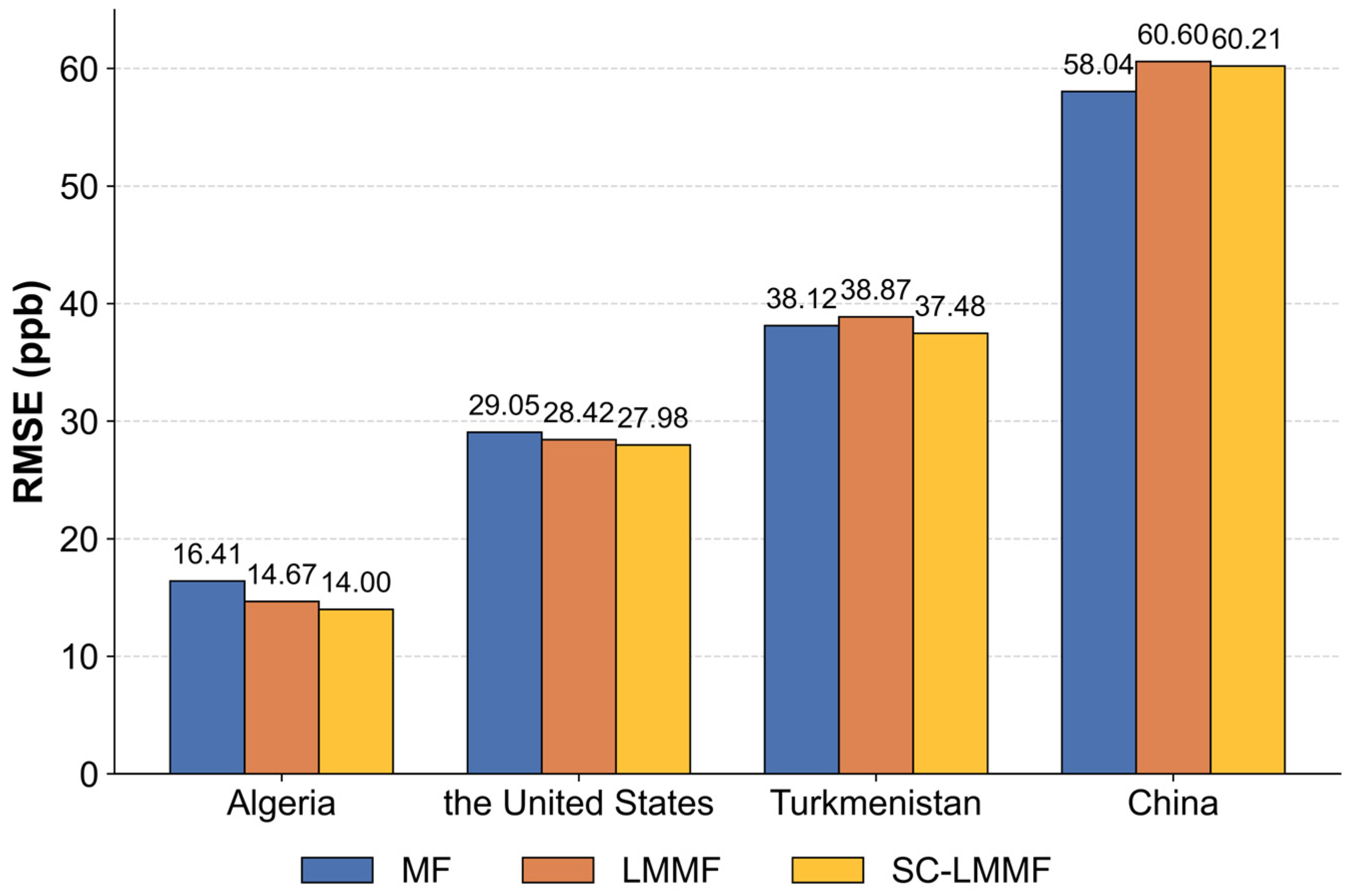
This characteristic can also be observed under low-emission conditions. Figure 11 compares the RMSE values of the three methods across the four regions at an emission rate of 500 kg/h. Overall, the differences among the three methods are smaller than those observed for the stronger plume cases in Figure 9. In Algeria and the United States, SC-LMMF still yields the lowest RMSE, although its relative advantage is limited. In Turkmenistan and China, the error levels of the three methods are relatively close. This indicates that when emissions are weak and plume enhancements approach the background noise level, retrieval errors are influenced to a greater extent by observational noise and surface background conditions, whereas the effect of nonlinear absorption errors at high concentrations becomes relatively weaker. Therefore, the improvement achieved by SC-LMMF under weak-plume conditions is reduced compared with that under stronger plume conditions.
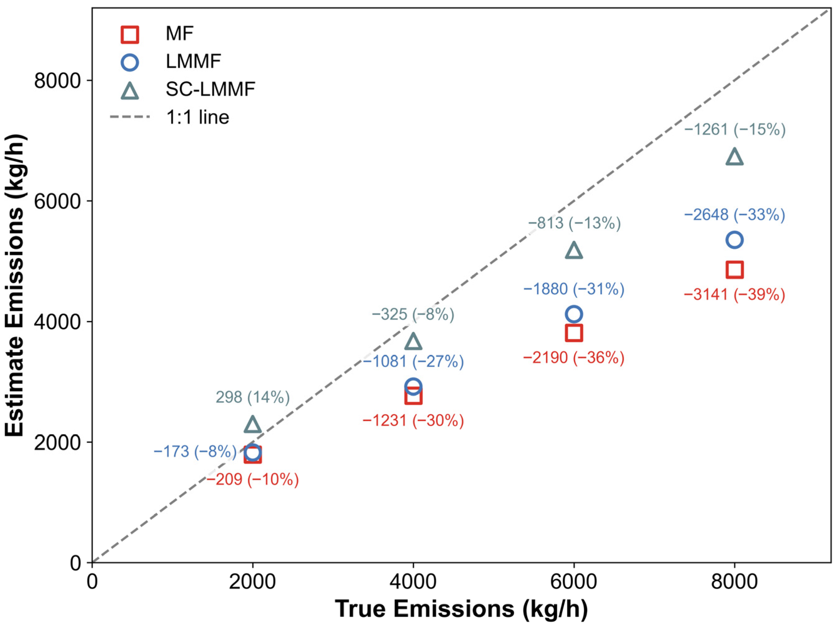
Figure 12 further presents the emission estimates for the United States region under different true emission rates. Overall, the emission estimates from all three methods increase with increasing true emission rate, but the degree of underestimation differs substantially among the methods. Under relatively low emission rates, the differences among the methods are less pronounced because plume enhancements are weaker and the number of statistically significant plume pixels available for emission estimation is limited. As the emission rate increases, the underestimation in MF and LMMF becomes increasingly severe. For example, at 8000 kg/h, the underestimation reaches 39% and 33% for MF and LMMF, respectively, whereas the bias of SC-LMMF is approximately 15%. This indicates that, under high-emission conditions, the residual underestimation of concentration enhancements in MF and LMMF is further propagated into the emission estimates, thereby leading to a more pronounced negative bias. In contrast, SC-LMMF can substantially mitigate this accumulation of bias.
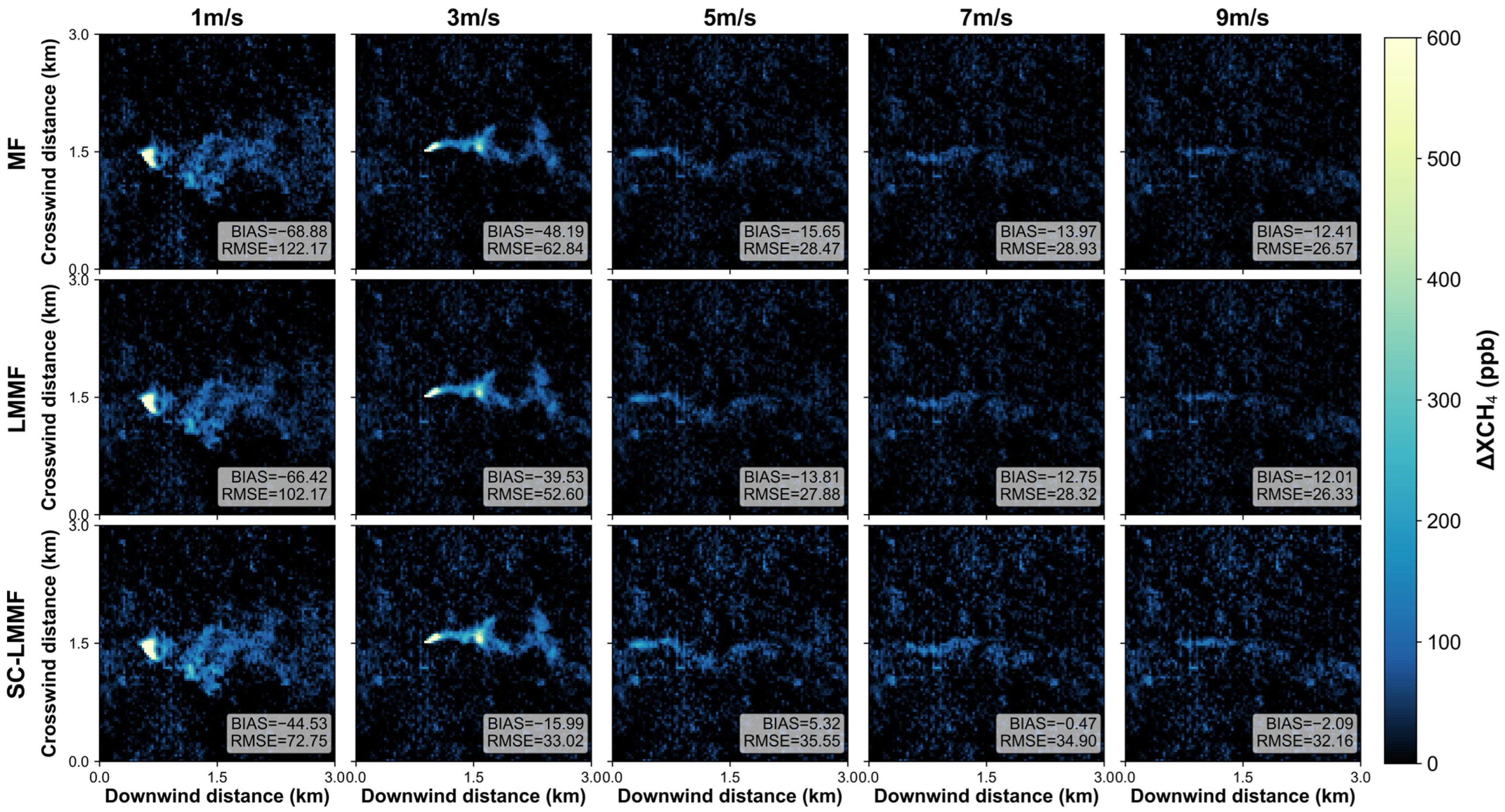
In addition to emission rate, wind speed is also an important factor affecting plume retrieval and emission estimation. Figure 13 presents the retrieval results for the United States region under different wind speed conditions. Overall, under low-wind conditions, plume enhancements are more concentrated, and the retrieved column enhancement amplitudes are correspondingly higher for all three methods. Under these conditions, the correction of the systematic underestimation in MF and the improvement in retrieval accuracy by LMMF and SC-LMMF are more evident, particularly as reflected by the progressive reductions in BIAS and RMSE. As wind speed increases, the plume gradually disperses, the column enhancement decreases, and the differences among the three methods become correspondingly smaller. At higher wind speeds, especially above 7 m/s, the absolute value of the bias decreases further, indicating that the systematic bias is reduced. However, the RMSE does not decrease accordingly, suggesting that under high-wind conditions, although the overall underestimation is alleviated, random errors and the uncertainty introduced by plume dispersion still have a substantial impact on the retrieval results.
Overall, the end-to-end simulation results indicate that MF, LMMF, and SC-LMMF exhibit consistent patterns across different regions, emission rates, and wind speed conditions. LMMF effectively alleviates the systematic underestimation inherent in the conventional MF, while SC-LMMF, by introducing a spectral-consistency constraint, further reduces the nonlinear systematic bias caused by differences in surface reflectance characteristics and atmospheric conditions. This improvement is more pronounced under moderate-to-high enhancement conditions, whereas the differences among the three methods become much smaller under weak-plume or complex-background conditions, where retrieval accuracy is more strongly influenced by background noise and surface heterogeneity.

3.4. Results of the Controlled-Release Experiment

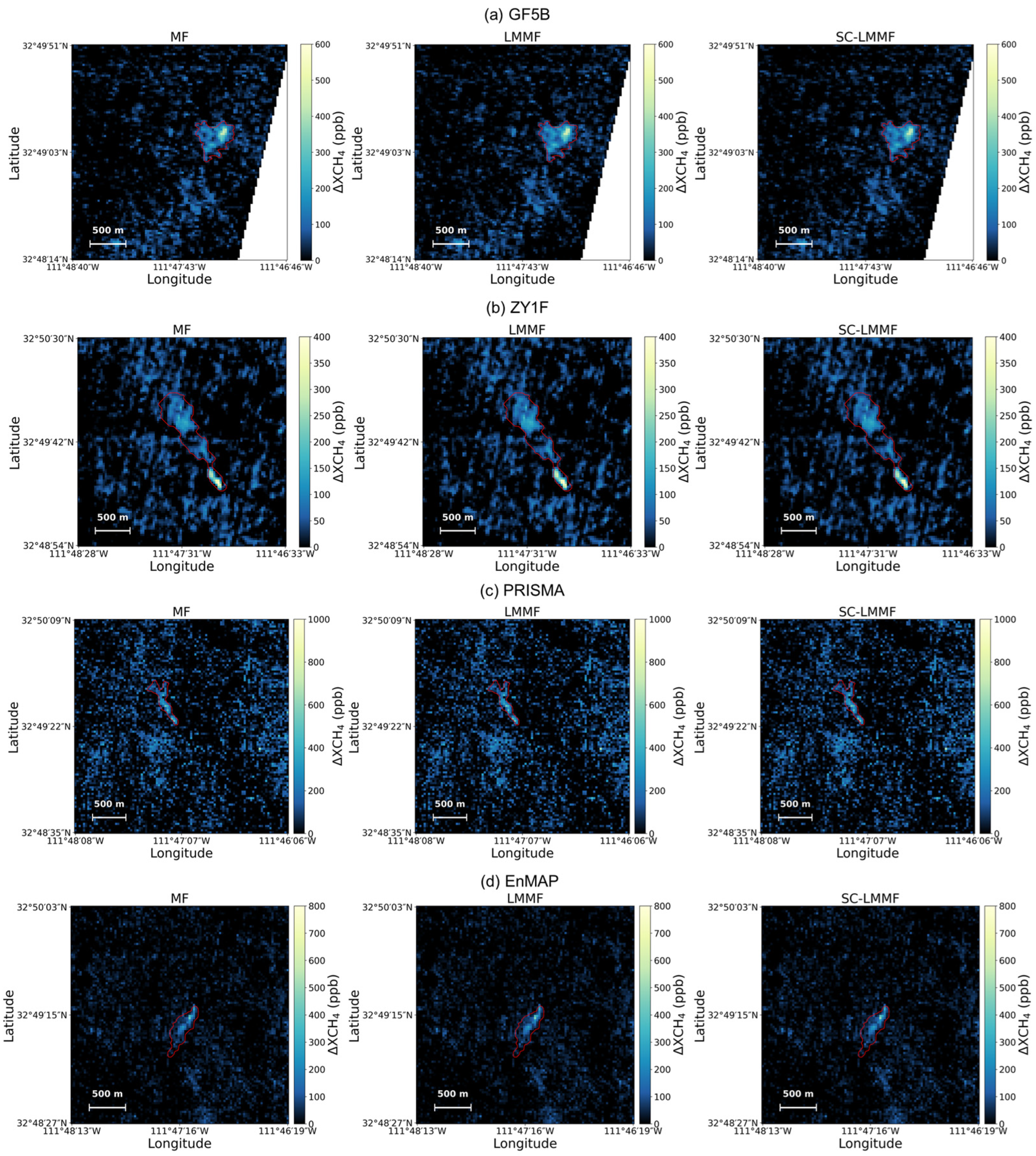
Based on the hyperspectral observations acquired during the Stanford controlled methane release campaign by the GF5B, ZY1F, PRISMA, and EnMAP satellites, a systematic comparison of the MF, LMMF, and SC-LMMF algorithms was conducted for plume retrieval and emission rate estimation. Figure 14 presents the spatial retrieval results under different satellite observation conditions.
From a spatial perspective, methane enhancement regions consistent with the controlled-release source location are identifiable in all four scenes, indicating that under relatively strong emission conditions, all three algorithms possess basic plume detection capabilities. The retrieved plume axes and overall dispersion patterns are generally consistent across the methods. To ensure a fair comparison, a common plume mask was applied for the subsequent quantitative analysis.
Nevertheless, due to systematic underestimation, the plume signals retrieved by the MF exhibit lower contrast and reduced spatial continuity. The LMMF mitigates this issue, leading to stronger methane enhancement signals in the plume core region and improved spatial coherence of the plume structure. This improvement is particularly evident in the GF5B results, where high-enhancement regions become more distinguishable. Building upon this improvement, the SC-LMMF further addresses the spectral inconsistencies induced by surface reflectance variability and atmospheric differences through dynamic UAS correction. Compared with the LMMF, the SC-LMMF slightly suppresses background variability, contributing to a more distinct enhancement pattern. However, because the controlled-release plume signals are relatively strong, the additional spatial improvement in plume morphology is modest.
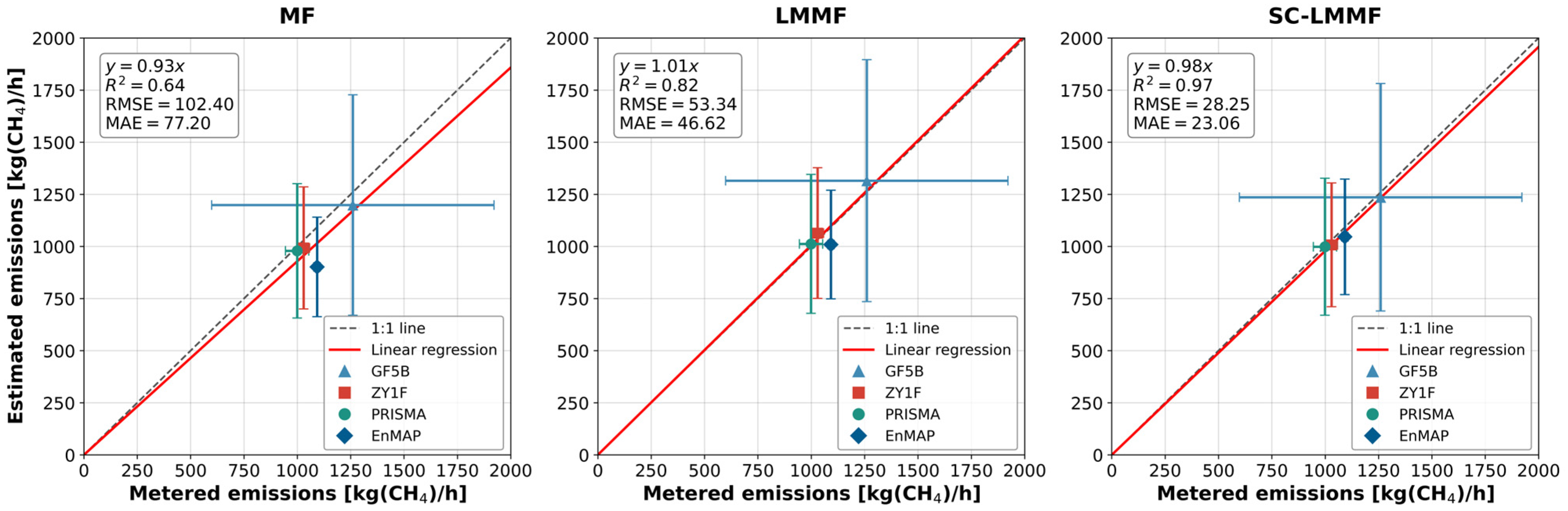
After plume delineation, the methane emission rates were further quantified using the IME method. The wind field data were obtained from in situ ground measurements at the experimental site. Figure 15 presents the quantitative comparison between the estimated emission rates and the metered release rates, with the uncertainties including both retrieval error and wind-speed error.
The emission rate results exhibit progressive improvements consistent with those observed in the plume retrieval stage. The MF method shows a distinct systematic underestimation, with a regression slope of 0.93 and an R2 of 0.64. The LMMF partially alleviates this bias, increasing the regression slope to 1.01 and improving the R2 to 0.82. Meanwhile, the RMSE and MAE are reduced by approximately 40%, indicating enhanced overall consistency. However, although the regression slope approaches the ideal 1:1 relationship, the LMMF results exhibit a slight overestimation for the GF5B, ZY1F, and PRISMA datasets, whereas the EnMAP results still show a residual underestimation.
Building upon this, the SC-LMMF further corrects the biases in the emission rate estimations. For the GF5B, ZY1F, and PRISMA data, the SC-LMMF mitigates the overestimation observed in the LMMF, yielding estimates more consistent with the metered release rates. For the EnMAP data, the SC-LMMF further reduces the remaining underestimation. Although the regression slope of the SC-LMMF is 0.97, its R2 reaches 0.98, and both the RMSE and MAE are further reduced—by approximately 70% relative to the MF—indicating improved stability and quantitative consistency.
Overall, the controlled-release experiments demonstrate that the improvements achieved at the plume retrieval stage can be effectively carried over to emission-rate quantification. LMMF mitigates the systematic underestimation inherent in MF, while SC-LMMF further reduces the systematic biases associated with observational and environmental variability, thereby exhibiting higher stability and consistency under multisource hyperspectral observations. The validation results from the four platforms—GF5B, ZY1F, PRISMA, and EnMAP—demonstrate that the proposed methods show a broadly consistent improvement trend across different satellite platforms. For the plume signals considered in this controlled-release experiment, the advantages of LMMF and SC-LMMF are not primarily reflected in whether the plume can be detected, but rather in enhanced plume contrast, improved spatial continuity, and better consistency in emission-rate estimation. It should be noted that, because different platforms vary in spectral resolution, spatial resolution, SNR, and observation geometry, the specific form of the algorithmic gain is not exactly the same across platforms; nevertheless, it is consistently manifested as reduced systematic bias and improved quantitative robustness. These results indicate that the proposed methods provide reliable methodological support for the stable detection and quantitative monitoring of methane point-source emissions using multisource satellite observations.

3.5. Computational Efficiency and Complexity Analysis

To comprehensively evaluate the operational applicability of the proposed methods, we quantitatively analyzed the computational costs of the MF, LMMF, and SC-LMMF algorithms. To ensure robustness and cross-sensor comparability, we directly adopted the 100 × 100 pixel retrieval test regions from the four representative hyperspectral satellites used in the controlled-release experiments, namely GF5B, ZY1F, PRISMA, and EnMAP, and used them as a unified benchmark for processing-time statistics. All tests were conducted sequentially in a single-thread Python 3.8.20 environment on the same hardware platform (AMD Ryzen 7 7735H CPU, 3.20 GHz, 32 GB RAM). The quantitative comparison results are summarized in Table 5.
As shown in Table 5, the conventional MF algorithm exhibits very high computational efficiency, with an average processing time of only 0.0209 s across the four platforms. By contrast, to more accurately characterize the nonlinear Beer-Lambert absorption process, the LMMF performs computationally intensive nonlinear iterative optimization for each pixel, increasing the average processing time to 2.7902 s. Some variation in runtime is observed among different satellite platforms, with PRISMA and GF5B showing relatively higher processing times, while EnMAP and ZY1F are comparatively lower. This difference is mainly related to the number of effective spectral bands involved in the retrieval within the SWIR absorption window: a larger number of effective bands leads to a higher-dimensional Jacobian matrix in the nonlinear optimization, thereby increasing the computational burden. The average processing time of SC-LMMF is 2.9220 s, only slightly higher than that of LMMF. This additional cost mainly arises from the dynamic matching process of the UAS LUT.
Overall, extending the retrieval framework from a linear model to a nonlinear model inevitably results in a substantial increase in computation time. However, this loss in efficiency is accompanied by stronger physical consistency and higher retrieval accuracy, indicating a clear trade-off between accuracy and efficiency. For large-scale rapid screening tasks, MF still has a significant advantage in computational efficiency. In contrast, for applications requiring higher quantitative accuracy and stronger adaptability to complex observational conditions, LMMF and SC-LMMF are more valuable. Furthermore, in practical deployments, the computational cost can be reduced by using high-performance computing platforms or parallel processing strategies. A hierarchical processing scheme may also be adopted, in which the highly efficient MF is first used for anomaly detection and preliminary plume screening over large areas, and the computationally intensive SC-LMMF is then applied only to the identified candidate plume regions, thereby achieving higher retrieval accuracy while maintaining overall processing efficiency.

4. Discussion

A synthesis of the UAS sensitivity analysis, idealized simulations, noise-perturbed simulations, end-to-end simulations, and controlled-release experiments indicates that the systematic underestimation of methane enhancements by the conventional MF under high-concentration conditions does not arise from a single invalid algorithmic assumption. Rather, it results from the combined effects of multiple physical processes and statistical estimation errors. These primarily include linearization errors associated with the exponential absorption process, contamination of background statistics by plume pixels, and systematic biases introduced by an inaccurate UAS. Under complex observational conditions, these error sources interact and may amplify one another, thereby constraining the quantitative accuracy of methane retrieval.
To address these error mechanisms, the proposed framework introduces targeted corrections at two levels: the observation model and the UAS representation. The UAS sensitivity analysis demonstrates that its numerical characteristics are jointly modulated by variations in optical path length and atmospheric state, providing a physical basis for constructing a dynamic spectral correction scheme. Results from both idealized and noise-perturbed simulations confirm the necessity of algorithmic refinement. The MF simplifies the radiative transfer process, which follows exponential attenuation, into a linear model, inevitably leading to systematic underestimation in high-concentration regions due to saturation effects. The LMMF preserves the exponential absorption formulation and employs Levenberg–Marquardt iterative optimization to solve the resulting nonlinear problem, thereby correcting the linearization error at the model-structure level. Building upon this, the SC-LMMF incorporates a lookup-table-based dynamic matching mechanism for the UAS, constraining uncertainties in spectral representation and reducing environmentally induced systematic biases. It should be noted that although MF exhibit strong robustness in plume detection, quantitative retrieval accuracy depends critically on the combined effects of nonlinear absorption modeling and adaptive spectral parameter correction. The results indicate that the SC-LMMF achieves improved control of systematic bias. However, its ability to suppress random noise remains limited, suggesting that the signal-to-noise ratio (SNR) of observations continues to be a fundamental constraint on hyperspectral gas quantification. The end-to-end simulations and controlled-release experiments further demonstrate the applicability and stability of the proposed methods under realistic and complex observational conditions. Compared with idealized simulations, real satellite observations involve more diverse error sources, which tend to amplify the biases associated with linear absorption approximations and fixed UAS assumptions. By reformulating the observation model, the LMMF improves structural physical consistency. Building upon this foundation, the SC-LMMF further introduces LUT-based spectral consistency constraints, thereby enhancing cross-scene and cross-sensor adaptability.
The comprehensive evaluation results highlight the differentiated applicability of LMMF and SC-LMMF under different levels of observational complexity. In routine scenes where observational conditions remain close to the baseline configuration, LMMF is generally sufficient to achieve high quantitative accuracy while maintaining relatively low computational cost. Under more complex observational conditions, however, SC-LMMF provides a more reliable solution because its dynamic UAS matching better constrains spectral mismatch errors and improves the control of systematic bias. According to the computational-efficiency analysis, the additional computational cost of SC-LMMF relative to LMMF is limited, indicating that this enhanced correction is still acceptable in practical applications. Therefore, the retrieval strategy can be selected flexibly according to observational complexity and processing requirements: LMMF is suitable for routine applications with relatively stable conditions, whereas SC-LMMF is more advantageous for consistent quantitative retrieval in complex scenes.
In addition, it should be noted that the background radiance mean and covariance matrix in this study are estimated from background pixels within the same scene and therefore can, to a certain extent, reflect the combined influence of solar geometry, surface elevation, and atmospheric state on background radiative transfer under the current observational conditions. Since matched-filter-based methods fundamentally identify methane enhancements through the radiance anomaly or statistical deviation of plume pixels relative to non-plume background pixels, rather than relying directly on absolute radiance values, this scene-based statistical representation of the background is generally reasonable for local retrievals within a single scene, where background pixels usually provide a good representation of the non-emission state and spatial variations in SZA and surface elevation remain limited. However, this approach still relies on the assumption that the background remains relatively stable within the local area. In practice, the surface is often composed of mixtures of vegetation, bare soil, and anthropogenic structures, leading to pronounced mixed-pixel effects. When the background statistical model fails to adequately separate surface endmember contributions, intrinsic spectral variability may be misinterpreted as methane absorption features. For weak point-source emissions, such background-induced radiance variations may be comparable to or even exceed the actual methane enhancement signal, resulting in biased concentration estimates and potential false plume detections. Although previous studies have attempted to mitigate surface heterogeneity effects through sparse priors and background spectral reconstruction techniques, their general applicability across regions, sensors, and complex surface conditions remains to be further evaluated [41,43,55]. Improving background spectral modeling and mitigating surface-induced errors therefore remain important directions for advancing high-precision point-source retrieval.
Beyond concentration retrieval accuracy, accurate quantification of emission rates remains subject to multiple uncertainties. Plume delineation errors and wind field uncertainty constitute the primary limiting factors. On the one hand, the accuracy of plume mask extraction directly determines the integration domain for emission estimation. Although the SC-LMMF enhances plume-background contrast and reduces misclassification, plume boundaries may become diffuse and morphologically unstable under low wind speed or strong turbulence conditions. As a result, low-concentration edge pixels may be omitted, introducing cumulative integration bias. On the other hand, emission quantification based on the IME method is highly sensitive to effective wind speed. While wind observations were relatively accurate in the controlled-release experiment, operational satellite applications often rely on reanalysis datasets such as ERA5 and GEOS-FP, whose uncertainties may reach approximately 50% [22,28], thereby becoming a dominant source of error in emission rate estimation.
In addition to the error sources introduced by external observational conditions, the proposed methods themselves still have several inherent limitations. First, the computational cost increases substantially. Compared with the fast matrix-based implementation of the conventional linear MF, both LMMF and SC-LMMF involve pixel-wise nonlinear iterative optimization, leading to a significant increase in overall processing time. SC-LMMF further adds a unit absorption spectrum lookup-table matching step on top of LMMF, resulting in additional computational overhead. Although the extra runtime of SC-LMMF relative to LMMF is limited, the overall computational burden of the nonlinear retrieval framework remains much higher than that of MF, which may constrain its real-time applicability for large-area monitoring and high-resolution operational deployment. Second, the effectiveness of the spectral correction depends on the simulation accuracy of the radiative transfer model and the quality of the lookup table construction. For example, in the current LUT design, AOD is moderately simplified in order to balance computational efficiency with sensitivity to the core geometric parameters. For most routine observational scenarios, this simplification is reasonable because the SWIR region is relatively less sensitive to background aerosols. However, under extreme aerosol conditions, such as intense dust storms, dense biomass-burning smoke, or severe industrial haze, AOD may exert a non-negligible influence on the radiance spectra reaching the sensor and on the representation of the UAS by altering path radiance, scattering contributions, and effective optical path length [56,57]. In such cases, the current simplification of AOD in the LUT may no longer be sufficient, and the dynamically matched UAS may still deviate from the actual state, thereby weakening the effectiveness of the spectral correction.
Future work will focus on several directions. First, computational efficiency can be improved through parallel computing, dimensionality reduction strategies, or region-adaptive processing frameworks to enhance operational feasibility. Second, the parameter space of the UAS LUT should be further expanded, particularly by incorporating key aerosol optical parameters such as aerosol type and single-scattering albedo, and by exploring adaptive LUT construction under different regions, seasons, atmospheric backgrounds, and extreme meteorological conditions, so as to improve the general applicability of the model under more variable environments. Finally, further efforts are required to address key practical error sources, including improving spectral modeling over heterogeneous surfaces, enhancing detection stability for weak plumes, and integrating high-accuracy local wind field data to reduce uncertainties in emission rate retrieval.

5. Conclusions

This study addresses the systematic underestimation of methane enhancements by the MF under high-concentration conditions in hyperspectral methane point-source retrieval. Focusing on two critical components—the observation model and spectral correction—this work systematically analyzes existing limitations and proposes corresponding methodological improvements. Specifically, the LMMF is developed by incorporating iterative nonlinear optimization into the MF framework. Building upon this, the SC-LMMF is further proposed by introducing a dynamic UAS correction scheme to enhance retrieval stability and consistency across varying emission strengths and multi-sensor observation conditions.
Comprehensive validation through idealized simulations, noise-perturbed simulations, end-to-end simulations, and controlled-release experiments demonstrates that the LMMF effectively mitigates the systematic underestimation of the MF under strong emission scenarios, substantially improving the linear consistency between retrieved and true methane enhancements. On this basis, the SC-LMMF further reduces systematic biases induced by variations in observation geometry, surface elevation, and atmospheric state through dynamic UAS correction. Consequently, retrieval results exhibit improved statistical stability and quantitative consistency across multi-source hyperspectral datasets. Under both simulated and real satellite observation conditions, the SC-LMMF consistently outperforms the LMMF and the conventional MF.
The findings indicate that enforcing physical consistency in both the observation model and key intermediate spectral parameters is essential for improving the reliability of MF-based methane point-source retrieval. The LMMF and SC-LMMF provide a tiered retrieval strategy tailored to different levels of observational complexity: the former achieves stable performance with lower computational cost when observation conditions are close to the baseline configuration, whereas the latter provides enhanced systematic bias control under complex observation environments. Nevertheless, compared with the conventional linear MF, the nonlinear iterative optimization and lookup-table matching introduced in the proposed methods increase the computational demand. In addition, further refinement of the spectral correction parameterization is still warranted. For large-scale, high-resolution applications, improvements in numerical efficiency and adaptive parameter construction strategies will be necessary.
Overall, the proposed LMMF and SC-LMMF provide a systematic and transferable methodological framework for stable detection and quantitative retrieval of methane point sources using multi-source hyperspectral satellite observations. These methods offer important methodological support for future multi-satellite methane emission monitoring, inventory verification, and refined mitigation assessment, and contribute to advancing hyperspectral remote sensing applications in greenhouse gas monitoring.

Author Contributions

Conceptualization, Z.H., Y.M., Z.L., Y.Z. and Z.S.; methodology, Z.H., Y.Z., C.L. and Q.Y.; software, Z.H. and T.L.; validation, Z.H. and L.Q.; formal analysis, Z.H., Y.M. and Z.Z.; investigation, Z.H., Y.G., X.Y. and X.L.; resources, Z.L., C.F. and Y.M.; data curation, Z.H. and T.L.; writing—original draft preparation, Z.H.; writing—review and editing, Y.M. and Z.L.; visualization, Z.H.; supervision, Y.M. and Z.L.; project administration, Z.L. and C.F.; funding acquisition, Z.L. and C.F. All authors have read and agreed to the published version of the manuscript.

Funding

This research was funded by the National Key R&D Program of China, grant number 2023YFB3907405.

Data Availability Statement

Data will be made available upon request.

Acknowledgments

The authors acknowledge the China Centre for Resources Satellite Data and Application for providing access to the GF5B and ZY1F satellite data used in this study. The authors also thank the Italian Space Agency for providing the PRISMA data and the German Aerospace Center for supplying the EnMAP data. Furthermore, the authors acknowledge the contributors of the Stanford controlled-release experiments for providing the emission measurements and ground-based meteorological data.

Conflicts of Interest

The authors declare no conflicts of interest.

Abbreviations

The following abbreviations are used in this manuscript:
MFMatched filter
LMMFLevenberg–Marquardt matched filter
SC-LMMFSpectrally corrected Levenberg–Marquardt matched filter
UASUnit absorption spectrum
ΔXCH4Methane column concentration enhancement
R2Coefficient of determination
RMSERoot mean square error
MAEMean absolute error
CH4Methane
CO2Carbon dioxide
GWPGlobal warming potential
SWIRShortwave infrared
SSRMFSparse Spectral Reconstruction Enhanced Matched Filter
LMFLognormal matched filter
IMFIterative matched filter
ILMFIterative lognormal matched filter
MLMFMulti-level matched filter
LMLevenberg–Marquardt
LUTLookup table
MODTRANMODerate Resolution Atmospheric TRANsmission
SRFSpectral response function
VZASatellite zenith angle
SZASolar zenith angle
AODAerosol optical depth
TTropical
MLSMid-latitude summer
MLWMid-latitude winter
SASSub-Arctic summer
SAWSub-Arctic winter
USU.S. Standard Atmosphere
IMEIntegrated mass enhancement
LESLarge eddy simulation
WRFWeather Research and Forecasting
TOATop-of-Atmosphere
AHSIAdvanced Hyperspectral Imager
CVCoefficient of variation

References

  1. US EPA. Understanding Global Warming Potentials. Available online: https://www.epa.gov/ghgemissions/understanding-global-warming-potentials (accessed on 13 July 2022).
  2. Isaksen, I.S.A.; Berntsen, T.K.; Dalsøren, S.B.; Eleftheratos, K.; Orsolini, Y.; Rognerud, B.; Stordal, F.; Søvde, O.A.; Zerefos, C.; Holmes, C.D. Atmospheric Ozone and Methane in a Changing Climate. Atmosphere 2014, 5, 518–535. [Google Scholar] [CrossRef] [Scilit]
  3. Saunois, M.; Stavert, A.R.; Poulter, B.; Bousquet, P.; Canadell, J.G.; Jackson, R.B.; Raymond, P.A.; Dlugokencky, E.J.; Houweling, S.; Patra, P.K.; et al. The Global Methane Budget 2000–2017. Earth Syst. Sci. Data 2020, 12, 1561–1623. [Google Scholar] [CrossRef] [Scilit]
  4. UNEP. Global Methane Assessment: Benefits and Costs of Mitigating Methane Emissions; United Nations Environment Programme: Nairobi, Kenya, 2021. [Google Scholar]
  5. IEA. The Global Methane Pledge—Global Methane Tracker. 2022. Available online: https://www.iea.org/reports/global-methane-tracker-2022/the-global-methane-pledge (accessed on 1 August 2022).
  6. Lelieveld, J.; Crutzen, P.J.; Dentener, F.J. Changing Concentration, Lifetime and Climate Forcing of Atmospheric Methane. Tellus B 1998, 50, 128–150. [Google Scholar] [CrossRef] [Scilit]
  7. Kirschke, S.; Bousquet, P.; Ciais, P.; Saunois, M.; Canadell, J.G.; Dlugokencky, E.J.; Bergamaschi, P.; Bergmann, D.; Blake, D.R.; Bruhwiler, L.; et al. Three Decades of Global Methane Sources and Sinks. Nat. Geosci. 2013, 6, 813–823. [Google Scholar] [CrossRef] [Scilit]
  8. Cusworth, D.H.; Duren, R.M.; Thorpe, A.K.; Tseng, E.; Thompson, D.; Guha, A.; Newman, S.; Foster, K.T.; Miller, C.E. Using Remote Sensing to Detect, Validate, and Quantify Methane Emissions from California Solid Waste Operations. Environ. Res. Lett. 2020, 15, 054012. [Google Scholar] [CrossRef] [Scilit]
  9. Qin, K.; He, Q.; Kang, H.; Hu, W.; Lu, F.; Cohen, J. Research Progress and Prospect of Satellite Remote Sensing of Methane Emissions in Coal Industry. Acta Opt. Sin. 2023, 43, 1899908–1899913. (In Chinese) [Google Scholar] [CrossRef] [Scilit]
  10. Duren, R.M.; Thorpe, A.K.; Foster, K.T.; Rafiq, T.; Hopkins, F.M.; Yadav, V.; Bue, B.D.; Thompson, D.R.; Conley, S.; Colombi, N.K.; et al. California’s Methane Super-Emitters. Nature 2019, 575, 180–184. [Google Scholar] [CrossRef] [Scilit]
  11. Canadell, J.G.; Monteiro, P.M.; Costa, M.H.; Da Cunha, L.C.; Cox, P.M.; Eliseev, A.V.; Henson, S.; Ishii, M.; Jaccard, S.; Koven, C.; et al. 2021: Global Carbon and other Biogeochemical Cycles and Feedbacks. In Climate Change 2021: The Physical Science Basis. Contribution of Working Group I to the Sixth Assessment Report of the Intergovernmental Panel on Climate Change; Masson-Delmotte, V., Zhai, P., Pirani, A., Connors, S.L., Péan, C., Berger, S., Caud, N., Chen, Y., Goldfarb, L., Gomis, M.I., et al., Eds.; Cambridge University Press: Cambridge, UK; New York, NY, USA, 2021; pp. 673–816. [Google Scholar] [CrossRef] [Scilit]
  12. Zhao, C.; Andrews, A.E.; Bianco, L.; Eluszkiewicz, J.; Hirsch, A.; MacDonald, C.; Nehrkorn, T.; Fischer, M.L. Atmospheric Inverse Estimates of Methane Emissions from Central California. J. Geophys. Res. 2009, 114, D16302. [Google Scholar] [CrossRef] [Scilit]
  13. Jacob, D.J.; Turner, A.J.; Maasakkers, J.D.; Sheng, J.; Sun, K.; Liu, X.; Chance, K.; Aben, I.; McKeever, J.; Frankenberg, C. Satellite Observations of Atmospheric Methane and Their Value for Quantifying Methane Emissions. Atmos. Chem. Phys. 2016, 16, 14371–14396. [Google Scholar] [CrossRef] [Scilit]
  14. Jacob, D.J.; Varon, D.J.; Cusworth, D.H.; Dennison, P.E.; Frankenberg, C.; Gautam, R.; Guanter, L.; Kelley, J.; McKeever, J.; Ott, L.E.; et al. Quantifying Methane Emissions from the Global Scale down to Point Sources Using Satellite Observations of Atmospheric Methane. Atmos. Chem. Phys. 2022, 22, 9617–9646. [Google Scholar] [CrossRef] [Scilit]
  15. Li, Z.; Xie, Y.; Shi, Y.; Li, Q.; Cohen, J.; Zhang, Y.; Han, Y.; Xiong, W.; Liu, Y. Review of Synergistic Observation of Greenhouse Gases and Aerosols from Atmospheric Environment Satellites. J. Remote Sens. 2022, 26, 795–816. (In Chinese) [Google Scholar] [CrossRef] [Scilit]
  16. He, Z.; Li, Z.; Fan, C.; Zhang, Y.; Shi, Z.; Zheng, Y.; Gu, H.; Ma, J.; Zuo, J.; Han, Y.; et al. Review of Atmospheric Methane Satellite Sensors and Remote Sensing Algorithms. Acta Opt. Sin. 2023, 43, 1899904–1899917. (In Chinese) [Google Scholar] [CrossRef] [Scilit]
  17. Varon, D.J.; Jacob, D.J.; Hmiel, B.; Gautam, R.; Lyon, D.R.; Omara, M.; Sulprizio, M.; Shen, L.; Pendergrass, D.; Nesser, H.; et al. Continuous Weekly Monitoring of Methane Emissions from the Permian Basin by Inversion of TROPOMI Satellite Observations. Atmos. Chem. Phys. 2023, 23, 7503–7520. [Google Scholar] [CrossRef] [Scilit]
  18. Zhang, Y.; Gautam, R.; Pandey, S.; Omara, M.; Maasakkers, J.D.; Sadavarte, P.; Lyon, D.; Nesser, H.; Sulprizio, M.P.; Varon, D.J.; et al. Quantifying Methane Emissions from the Largest Oil-Producing Basin in the United States from Space. Sci. Adv. 2020, 6, eaaz5120. [Google Scholar] [CrossRef] [Scilit]
  19. Irakulis-Loitxate, I.; Gorroño, J.; Zavala-Araiza, D.; Guanter, L. Satellites Detect a Methane Ultra-Emission Event from an Offshore Platform in the Gulf of Mexico. Environ. Sci. Technol. Lett. 2022, 9, 520–525. [Google Scholar] [CrossRef] [Scilit]
  20. Sánchez-García, E.; Gorroño, J.; Irakulis-Loitxate, I.; Varon, D.J.; Guanter, L. Mapping Methane Plumes at Very High Spatial Resolution with the WorldView-3 Satellite. Atmos. Meas. Tech. 2022, 15, 1657–1674. [Google Scholar] [CrossRef] [Scilit]
  21. Gorroño, J.; Varon, D.J.; Irakulis-Loitxate, I.; Guanter, L. Understanding the Potential of Sentinel-2 for Monitoring Methane Point Emissions. Atmos. Meas. Tech. 2023, 16, 89–107. [Google Scholar] [CrossRef] [Scilit]
  22. Irakulis-Loitxate, I.; Guanter, L.; Liu, Y.-N.; Varon, D.J.; Maasakkers, J.D.; Zhang, Y.; Chulakadabba, A.; Wofsy, S.C.; Thorpe, A.K.; Duren, R.M.; et al. Satellite-Based Survey of Extreme Methane Emissions in the Permian Basin. Sci. Adv. 2021, 7, eabf4507. [Google Scholar] [CrossRef] [Scilit] [PubMed]
  23. Lu, T.; Li, Z.; Fan, C.; He, Z.; Jiang, X.; Zhang, Y.; Gao, Y.; Xuan, Y.; de Leeuw, G. Global Methane Retrieval, Monitoring, and Quantification in Hotspot Regions Based on AHSI/ZY-1 Satellite. Atmosphere 2025, 16, 510. [Google Scholar] [CrossRef] [Scilit]
  24. Guanter, L.; Irakulis-Loitxate, I.; Gorroño, J.; Sánchez-García, E.; Cusworth, D.H.; Varon, D.J.; Cogliati, S.; Colombo, R. Mapping Methane Point Emissions with the PRISMA Spaceborne Imaging Spectrometer. Remote Sens. Environ. 2021, 265, 112671. [Google Scholar] [CrossRef] [Scilit]
  25. Cusworth, D.H.; Jacob, D.J.; Varon, D.J.; Chan Miller, C.; Liu, X.; Chance, K.; Thorpe, A.K.; Duren, R.M.; Miller, C.E.; Thompson, D.R.; et al. Potential of Next-Generation Imaging Spectrometers to Detect and Quantify Methane Point Sources from Space. Atmos. Meas. Tech. 2019, 12, 5655–5668. [Google Scholar] [CrossRef] [Scilit]
  26. Thorpe, A.K.; Green, R.O.; Thompson, D.R.; Brodrick, P.G.; Chapman, J.W.; Elder, C.D.; Irakulis-Loitxate, I.; Cusworth, D.H.; Ayasse, A.K.; Duren, R.M.; et al. Attribution of Individual Methane and Carbon Dioxide Emission Sources Using EMIT Observations from Space. Sci. Adv. 2023, 9, eadh2391. [Google Scholar] [CrossRef] [Scilit]
  27. Duren, R.; Cusworth, D.; Ayasse, A.; Howell, K.; Diamond, A.; Scarpelli, T.; Kim, J.; O’neill, K.; Lai-Norling, J.; Thorpe, A.; et al. The Carbon Mapper Emissions Monitoring System. Atmos. Meas. Tech. 2025, 18, 6933–6958. [Google Scholar] [CrossRef] [Scilit]
  28. Varon, D.J.; Jacob, D.J.; Jervis, D.; McKeever, J. Quantifying Time-Averaged Methane Emissions from Individual Coal Mine Vents with GHGSat-D Satellite Observations. Environ. Sci. Technol. 2020, 54, 10246–10253. [Google Scholar] [CrossRef] [Scilit]
  29. Chan Miller, C.; Roche, S.; Wilzewski, J.S.; Liu, X.; Chance, K.; Souri, A.H.; Conway, E.; Luo, B.; Samra, J.; Hawthorne, J.; et al. Methane Retrieval from MethaneAIR Using the CO2 Proxy Approach: A Demonstration for the Upcoming MethaneSAT Mission. Atmos. Meas. Tech. 2024, 17, 5429–5454. [Google Scholar] [CrossRef] [Scilit]
  30. Liu, J.; Lan, Y.; Zhou, X.; Wang, Y. Xiguang-1 Hyperspectral Remote Sensing Satellite System and Applications. Satell. Appl. 2025, 6, 41–48. (In Chinese) [Google Scholar]
  31. He, Z.; Li, Z.; Ma, Y.; Zhang, Y.; Qie, L.; Fan, C.; Zhang, Z.; Gao, Y.; Cai, Q.; Lu, T.; et al. Atmospheric Methane Plume Detection and Remote Sensing Analysis of Point Source Emissions from Bikong-1 Satellite. Acta Opt. Sin. (Web) 2025, 2, 2215001. (In Chinese) [Google Scholar] [CrossRef] [Scilit]
  32. Han, G.; Pei, Z.; Shi, T.; Mao, H.; Li, S.; Mao, F.; Ma, X.; Zhang, X.; Gong, W. Unveiling Unprecedented Methane Hotspots in China’s Leading Coal Production Hub: A Satellite Mapping Revelation. Geophys. Res. Lett. 2024, 51, e2024GL109065. [Google Scholar] [CrossRef] [Scilit]
  33. Tong, H.; Cheng, T.; Li, X.; Zhu, H.; Ye, X.; Fan, D.; Tang, T. Reduction of Methane Emissions through Improved Landfill Management. Nat. Clim. Change 2025, 15, 866–872. [Google Scholar] [CrossRef] [Scilit]
  34. Dogniaux, M.; Maasakkers, J.D.; Girard, M.; Jervis, D.; McKeever, J.; Schuit, B.J.; Sharma, S.; Lopez-Noreña, A.; Varon, D.J.; Aben, I. Global Satellite Survey Reveals Uncertainty in Landfill Methane Emissions. Nature 2025, 647, 397–402. [Google Scholar] [CrossRef] [Scilit]
  35. Jervis, D.; Girard, M.; MacLean, J.-P.W.; Marshall, D.; McKeever, J.; Strupler, M.; Ramier, A.; Tarrant, E.; Young, D.; Maasakkers, J.D.; et al. Global Energy Sector Methane Emissions Estimated by Using Facility-Level Satellite Observations. Science 2025, 390, 1151–1155. [Google Scholar] [CrossRef] [Scilit] [PubMed]
  36. Jervis, D.; McKeever, J.; Durak, B.O.A.; Sloan, J.J.; Gains, D.; Varon, D.J.; Ramier, A.; Strupler, M.; Tarrant, E. The GHGSat-D Imaging Spectrometer. Atmos. Meas. Tech. 2021, 14, 2127–2140. [Google Scholar] [CrossRef] [Scilit]
  37. Borchardt, J.; Gerilowski, K.; Krautwurst, S.; Bovensmann, H.; Thorpe, A.K.; Thompson, D.R.; Frankenberg, C.; Miller, C.E.; Duren, R.M.; Burrows, J.P. Detection and Quantification of CH4 Plumes Using the WFM-DOAS Retrieval on AVIRIS-NG Hyperspectral Data. Atmos. Meas. Tech. 2021, 14, 1267–1291. [Google Scholar] [CrossRef] [Scilit]
  38. Jongaramrungruang, S.; Matheou, G.; Thorpe, A.K.; Zeng, Z.-C.; Frankenberg, C. Remote Sensing of Methane Plumes: Instrument Tradeoff Analysis for Detecting and Quantifying Local Sources at Global Scale. Atmos. Meas. Tech. 2021, 14, 7999–8017. [Google Scholar] [CrossRef] [Scilit]
  39. Theiler, J. Absorptive Weak Plume Detection on Gaussian and Non-Gaussian Background Clutter. IEEE J. Sel. Top. Appl. Earth Obs. Remote Sens. 2021, 14, 6842–6854. [Google Scholar] [CrossRef] [Scilit]
  40. Funk, C.C.; Theiler, J.; Roberts, D.A.; Borel, C.C. Clustering to Improve Matched Filter Detection of Weak Gas Plumes in Hyperspectral Thermal Imagery. IEEE Trans. Geosci. Remote Sens. 2001, 39, 1410–1420. [Google Scholar] [CrossRef] [Scilit]
  41. Foote, M.D.; Dennison, P.E.; Thorpe, A.K.; Thompson, D.R.; Jongaramrungruang, S.; Frankenberg, C.; Joshi, S.C. Fast and Accurate Retrieval of Methane Concentration from Imaging Spectrometer Data Using Sparsity Prior. IEEE Trans. Geosci. Remote Sens. 2020, 58, 6480–6492. [Google Scholar] [CrossRef] [Scilit]
  42. Roger, J.; Guanter, L.; Gorroño, J.; Irakulis-Loitxate, I. Exploiting the Entire Near-Infrared Spectral Range to Improve the Detection of Methane Plumes with High-Resolution Imaging Spectrometers. Atmos. Meas. Tech. 2023, 17, 1333–1346. [Google Scholar] [CrossRef] [Scilit]
  43. Li, K.; Bai, K.; Fu, P.; Jiao, P.; Chen, H.; Huang, X.; Liu, C.; Chang, N.-B. SSRMF: A Sparse Spectral Reconstruction Enhanced Matched Filter for Improving Point-Source Methane Emission Detection in Complex Terrain. ISPRS J. Photogramm. Remote Sens. 2025, 225, 238–256. [Google Scholar] [CrossRef] [Scilit]
  44. Schaum, A. A Uniformly Most Powerful Detector of Gas Plumes against a Cluttered Background. Remote Sens. Environ. 2021, 260, 112443. [Google Scholar] [CrossRef] [Scilit]
  45. Kim, K.-E.; Lee, S.-S.; Baik, H.-S. Iterative Matched Filtering for Detection of Non-Rare Target Materials in Hyperspectral Imagery. In Proceedings of the Image and Signal Processing for Remote Sensing XXII; SPIE: Edinburgh, UK, 2016; Volume 10004, pp. 133–139. [Google Scholar]
  46. Pei, Z.; Han, G.; Mao, H.; Chen, C.; Shi, T.; Yang, K.; Ma, X.; Gong, W. Improving Quantification of Methane Point Source Emissions from Imaging Spectroscopy. Remote Sens. Environ. 2023, 295, 113652. [Google Scholar] [CrossRef] [Scilit]
  47. Liang, M.; Zhang, Y.; Chen, L.; Tao, J.; Fan, M.; Yu, C. An Effective Quantification of Methane Point-Source Emissions with the Multi-Level Matched Filter from Hyperspectral Imagery. Remote Sens. 2025, 17, 843. [Google Scholar] [CrossRef] [Scilit]
  48. Foote, M.D.; Dennison, P.E.; Sullivan, P.R.; O’Neill, K.B.; Thorpe, A.K.; Thompson, D.R.; Cusworth, D.H.; Duren, R.; Joshi, S.C. Impact of Scene-Specific Enhancement Spectra on Matched Filter Greenhouse Gas Retrievals from Imaging Spectroscopy. Remote Sens. Environ. 2021, 264, 112574. [Google Scholar] [CrossRef] [Scilit]
  49. Thompson, D.R.; Thorpe, A.K.; Frankenberg, C.; Green, R.O.; Duren, R.; Guanter, L.; Hollstein, A.; Middleton, E.; Ong, L.; Ungar, S. Space-Based Remote Imaging Spectroscopy of the Aliso Canyon CH4 Superemitter. Geophys. Res. Lett. 2016, 43, 6571–6578. [Google Scholar] [CrossRef] [Scilit]
  50. Berk, A.; Anderson, G.P.; Acharya, P.K.; Bernstein, L.S.; Muratov, L.; Lee, J.; Fox, M.; Adler-Golden, S.M.; Chetwynd, J.H.; Hoke, M.L.; et al. MODTRAN 5: A Reformulated Atmospheric Band Model with Auxiliary Species and Practical Multiple Scattering Options: Update. In Proceedings of the Algorithms and Technologies for Multispectral, Hyperspectral, and Ultraspectral Imagery XI; SPIE: Orlando, FL, USA, 2005; Volume 5806, pp. 662–667. [Google Scholar]
  51. Sherwin, E.D.; El Abbadi, S.H.; Burdeau, P.M.; Zhang, Z.; Chen, Z.; Rutherford, J.S.; Chen, Y.; Brandt, A.R. Single-Blind Test of Nine Methane-Sensing Satellite Systems from Three Continents. Atmos. Meas. Tech. 2024, 17, 765–782. [Google Scholar] [CrossRef] [Scilit]
  52. Sherwin, E.D.; Rutherford, J.S.; Chen, Y.; Aminfard, S.; Kort, E.A.; Jackson, R.B.; Brandt, A.R. Single-Blind Validation of Space-Based Point-Source Detection and Quantification of Onshore Methane Emissions. Sci. Rep. 2023, 13, 3836. [Google Scholar] [CrossRef] [Scilit]
  53. Talbot, C.; Bou-Zeid, E.; Smith, J. Nested Mesoscale Large-Eddy Simulations with WRF: Performance in Real Test Cases. J. Hydrometeorol. 2012, 13, 1421–1441. [Google Scholar] [CrossRef] [Scilit]
  54. Varon, D.J.; Jacob, D.J.; McKeever, J.; Jervis, D.; Durak, B.O.A.; Xia, Y.; Huang, Y. Quantifying Methane Point Sources from Fine-Scale Satellite Observations of Atmospheric Methane Plumes. Atmos. Meas. Tech. 2018, 11, 5673–5686. [Google Scholar] [CrossRef] [Scilit]
  55. Sun, E.; Wang, X.; Wu, S.; Ye, H.; Shi, H.; An, Y.; Li, C.; Jiang, Y. Improving Methane Point Sources Detection Over Heterogeneous Land Surface for Satellite Hyperspectral Imagery. IEEE J. Sel. Top. Appl. Earth Obs. Remote Sens. 2025, 18, 699–711. [Google Scholar] [CrossRef] [Scilit]
  56. Feng, C.; Chen, S.; Zeng, Z.-C.; Luo, Y.; Natraj, V.; Yung, Y.L. Aerosol-Calibrated Matched Filter Method for Retrievals of Methane Point Source Emissions over the Los Angeles Basin. Earth Space Sci. 2024, 11, e2024EA003519. [Google Scholar] [CrossRef] [Scilit]
  57. Huang, Y.; Natraj, V.; Zeng, Z.-C.; Kopparla, P.; Yung, Y.L. Quantifying the Impact of Aerosol Scattering on the Retrieval of Methane from Airborne Remote Sensing Measurements. Atmos. Meas. Tech. 2020, 13, 6755–6769. [Google Scholar] [CrossRef] [Scilit]
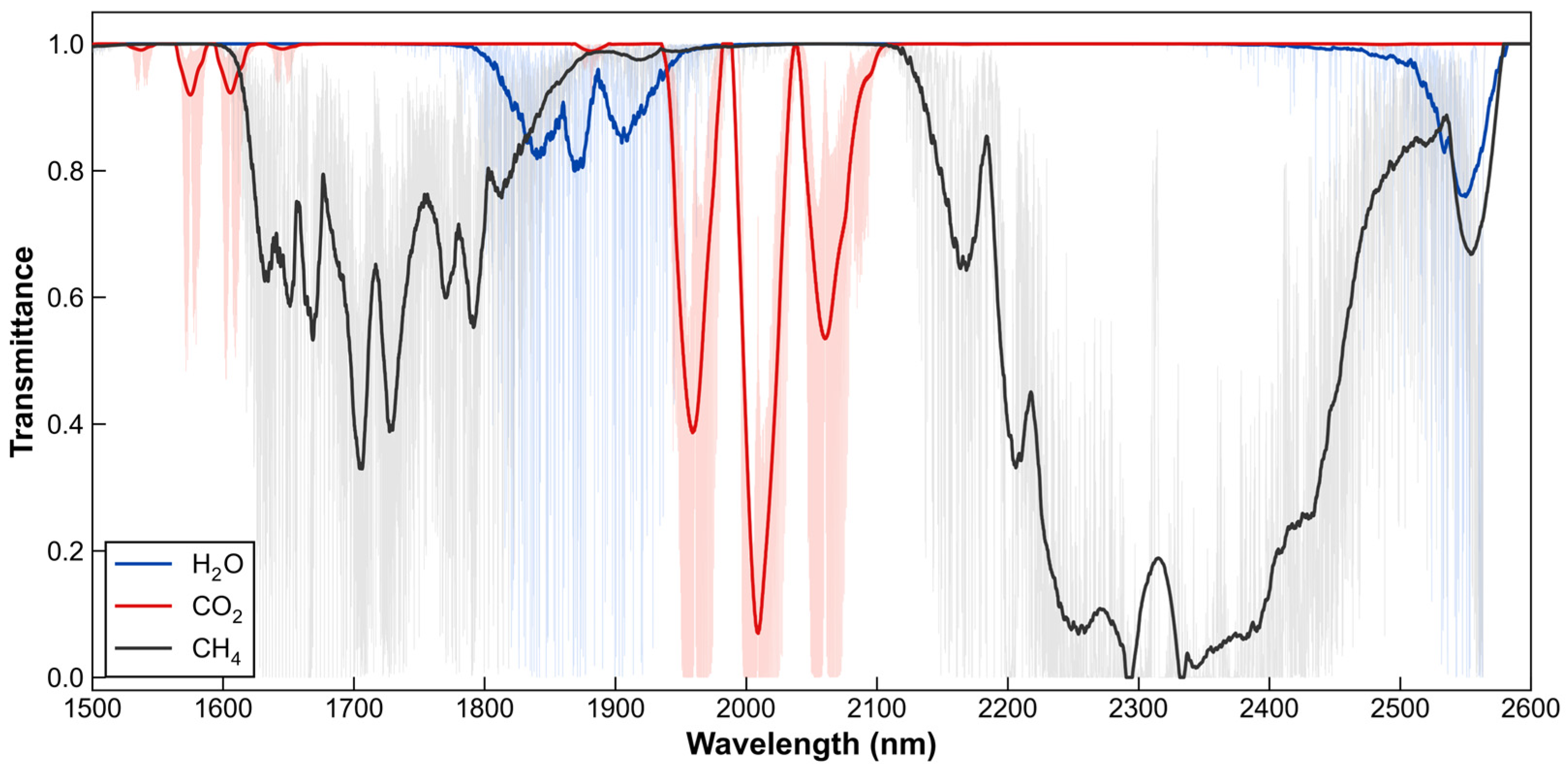
Figure 1. Atmospheric transmittance spectra of water vapor, carbon dioxide, and methane in the 1500–2600 nm spectral range. The light-colored thin lines represent the high-resolution transmittance spectra simulated using the HITRAN database, while the dark solid lines denote the absorption envelopes smoothed via a Savitzky–Golay filter, illustrating the macroscopic absorption characteristics of these gases over this wavelength range.
Remotesensing 18 01195 g001
Figure 2. Sensitivity of the methane unit absorption spectrum (UAS) to key parameters. (a) Solar zenith angle (SZA); (b) Surface elevation; (c) Aerosol optical depth (AOD); (d) Atmospheric profile.
Remotesensing 18 01195 g002
Figure 3. Methane plume simulated using WRF-LES, under a uniform westerly wind of 3 m/s with an emission rate of 2000 kg/h.
Remotesensing 18 01195 g003
Figure 4. Real AHSI TOA radiance data utilized in the end-to-end simulations. The upper row presents true-color composites of the four AHSI scenes. The red rectangles indicate the 100 × 100 pixel subregions where the simulated methane plumes were embedded, and the corresponding center coordinates are labeled in the lower-right corner of each upper-panel image. The lower row shows the corresponding TOA radiance at 2300 nm for each subregion. The coefficient of variation (CV), displayed in the lower-right corner of each panel, is calculated as the ratio of the standard deviation to the mean radiance at 2300 nm and quantitatively characterizes the surface spatial homogeneity.
Remotesensing 18 01195 g004
Figure 5. Quantitative scatter comparison of the retrieved versus true methane column concentration enhancements for the MF and LMMF algorithms under idealized observation conditions.
Remotesensing 18 01195 g005
Figure 6. Spatial distribution of the methane plumes retrieved by the MF and LMMF algorithms under noise-perturbed conditions, together with their difference within the plume region.
Remotesensing 18 01195 g006
Figure 7. Quantitative scatter comparison of the retrieved versus true methane column concentration enhancements for the MF and LMMF algorithms under noise-perturbed conditions.
Remotesensing 18 01195 g007
Figure 8. Reductions in BIAS and RMSE of SC-LMMF relative to LMMF under different observation conditions. (a) solar zenith angle; (b) surface elevation; (c) aerosol optical depth; (d) atmospheric profile. The arrow indicates that the value exceeds the axis scale.
Remotesensing 18 01195 g008
Figure 9. Quantitative scatter comparison of the retrieved versus true methane column concentration enhancements for the MF, LMMF, and SC-LMMF algorithms under the end-to-end simulations. Results are presented for four representative regions: (a) Algeria; (b) the United States; (c) Turkmenistan; (d) China.
Remotesensing 18 01195 g009
Figure 10. Q Histograms of retrieved ΔXCH4 for non-emission pixels in the United States region for the MF, LMMF, and SC-LMMF methods.
Remotesensing 18 01195 g010
Figure 11. Comparison of RMSE for the MF, LMMF, and SC-LMMF methods across four regions under a low-emission condition of 500 kg/h.
Remotesensing 18 01195 g011
Figure 12. Comparison of estimated versus true methane emission rates in the United States region for the MF, LMMF, and SC-LMMF methods under different emission-rate scenarios.
Remotesensing 18 01195 g012
Figure 13. Retrieval performance of the MF, LMMF, and SC-LMMF methods in the United States region under different wind speed conditions.
Remotesensing 18 01195 g013
Figure 14. Methane plume retrieval results from the controlled-release experiment. (a) GF5B/AHSI; (b) ZY1F/AHSI; (c) PRISMA/HYC; (d) EnMAP/HSI. Red boxes indicate the plume mask used for quantitative analysis.
Remotesensing 18 01195 g014
Figure 15. Quantitative comparison between estimated methane emission rates and metered emission rates in the controlled-release experiment. The black dashed line represents the 1:1 reference line, and the red solid line denotes the linear regression fit. The horizontal and vertical error bars indicate the uncertainties of the metered emission rates and the estimated emission rates, respectively.
Remotesensing 18 01195 g015
Table 1. Parameter settings for sensitivity analysis of the methane unit absorption spectrum.
ParameterBaseline ValueVariation RangeSampling Strategy
Solar Zenith Angle (SZA)35°0–70°Uniform sampling at 5° intervals
Surface Elevation0 km0–3 kmUniform sampling at 0.5 km intervals
Aerosol Optical Depth (AOD)0.30.1–2.0Non-uniform discrete sampling (0.1, 0.3, 0.5, 0.7, 1.0, 1.5, 2.0)
Atmospheric Profile *UST, MLS, MLW, SAS, SAW, USDiscrete standard atmospheric profiles
* Abbreviations: T (Tropical), MLS (Mid-Latitude Summer), MLW (Mid-Latitude Winter), SAS (Sub-Arctic Summer), SAW (Sub-Arctic Winter), US (U.S. Standard Atmosphere).
Table 2. Hyperspectral satellite scenes acquired during the controlled-release experiment and used for methane retrieval and emission quantification.
Satellite/SensorSWIR Spectral Resolution (nm)Spatial Resolution (m)Swath Width (km)Scene IDDateTime (UTC)
GF5B/AHSI103060GF5B_AHSI_W112.1_N32.8_20221115_006332_L1000023966315 November 202218:21
ZY1F/AHSI203060ZY1F_AHSI_W111.72_N33.06_20221026_004370_L1A000026565626 October 202218:23
PRISMA/HYC103030PRS_L1_STD_OFFL_20221130180952_20221130180956_000130 November 202218:09
EnMAP/HSI103030ENMAP01-____L1C-DT0000005368_20221116T184050Z_005_V010502_20250407T141831Z-SPECTRAL_IMAGE16 November 202218:40
Table 3. WRF-LES configuration parameters for the idealized methane plume simulation.
Parameter CategoryParameter Setting
Simulation toolWRF-LES (based on WRF v4.0, modified default LES case)
Terrain and atmospheric conditionsFlat terrain, cloud-free
Surface sensible heat flux100 W·m−2
Surface roughness length0.1 m
ForcingLarge-scale pressure gradient maintaining the momentum field
Boundary conditionsPeriodic lateral boundary conditions
Boundary layer configuration1000 m mixed layer with an inversion above; model top located 700 m above the inversion
Wind profileInitial uniform westerly wind, 3 m·s−1
Passive tracer setupSingle continuous point source with a normalized emission rate (scalable in post-processing)
Domain size12 km × 12 km
Horizontal resolution30 m × 30 m
Vertical resolution30 m
Simulation duration1 h
CH4 emission rate2000 kg·h−1
Table 4. Overview of the three simulation experiments.
Simulation ExperimentΔXCH4 GenerationSurface CharacteristicsInstrument Noise
Idealized simulationUniform sampling from 0 to 1400 ppb at 40 ppb intervalsNo surface reflectance consideredNo instrument noise
Noise-perturbed simulationWRF-LES-simulated ΔXCH4 fieldMixed soil and vegetation surface1% Gaussian noise
End-to-end simulationWRF-LES-simulated ΔXCH4 fieldReal GF5B/AHSI surface reflectanceRealistic AHSI noise characteristics
Table 5. Quantitative comparison of computational efficiency for different retrieval algorithms.
AlgorithmComputational Complexity CharacteristicsProcessing Time (s)Relative Cost
MFLinear projection (matrix multiplication)0.02091
LMMFNonlinear iterative optimization (pixel-wise)2.7902~134
SC-LMMFNonlinear iterative optimization + lookup-table matching2.9220~140
Disclaimer/Publisher’s Note: The statements, opinions and data contained in all publications are solely those of the individual author(s) and contributor(s) and not of MDPI and/or the editor(s). MDPI and/or the editor(s) disclaim responsibility for any injury to people or property resulting from any ideas, methods, instructions or products referred to in the content.