A Hyperspectral Simulation-Driven Framework for Sub-Pixel Impervious Surface Mapping: A Case Study Using Landsat Imagery

Highlights

What are the main findings?

• The results confirm the reliability of the simulated multispectral data, which show strong radiometric consistency with actual satellite observations.
• Experimental results demonstrate that the hyperspectral-derived simulation framework constructs a physically consistent spectrum–abundance training library, effectively enabling accurate sub-pixel impervious surface mapping.

What are the implications of the main findings?

• The framework establishes a physically consistent training library that mitigates sample noise and enhances sub-pixel impervious surface mapping accuracy by ensuring rigorous spectrum-abundance correspondence within simulated multispectral data.
• The methodology exhibits platform-independent adaptability, where sensor-specific training datasets are generated through spectral convolution, enabling accurate sub-pixel impervious surface mapping across different medium-resolution satellite sensors.

Abstract

The rapid advancement of global urbanization has rendered Impervious Surface Area (ISA) a critical indicator for monitoring urban ecological and thermal environments. However, traditional sub-pixel ISA estimation methods, such as Spectral Mixture Analysis (SMA) and machine learning regression, are significantly constrained by spectral variability and a scarcity of high-quality training samples. To address these limitations, this study proposes a novel sub-pixel Impervious Surface Fraction (ISF) retrieval framework leveraging high-resolution airborne hyperspectral data. By simulating physically consistent multispectral reflectance and generating high-accuracy reference ISF via spatial aggregation, we construct a robust and noise-resistant training dataset. Experimental results on Landsat data demonstrate that this simulation-based approach effectively mitigates sample uncertainty, significantly enhances retrieval accuracy, and accurately preserves spatial details and boundary structures. Theoretically, the framework exhibits strong cross-sensor adaptability, as it allows for the generation of sensor-consistent training datasets for various medium-resolution satellite platforms by simply substituting the target sensor’s spectral response functions. Combined with this inherent scalability and the potential for cross-sensor model migration, this method provides a reliable and systematic paradigm for long-term, high-precision ISF mapping across multiple satellite constellations.

1. Introduction

In the context of rapid global urbanization, impervious surface area (ISA) has emerged as a key indicator for characterizing urbanization intensity and urban environmental change. The expansion of ISA not only contributes to the formation and intensification of the urban heat island (UHI) effect but also alters urban hydrological processes, reduces ecological connectivity, and degrades ecosystem services [1,2,3]. Consequently, the precise quantification of ISA holds profound scientific significance. Owing to its extensive temporal archive and global coverage, the Landsat satellite series has served as a primary high-quality data source for long-term ISA mapping [4,5]. However, urban landscapes are inherently characterized by high heterogeneity and spatial fragmentation. In such complex environments, the “mixed pixel” phenomenon is prevalent within medium-resolution imagery (e.g., 30 m), which makes traditional pixel-level hard classification methods inadequate for meeting high-precision monitoring requirements [6,7]. To address this challenge, estimating sub-pixel impervious surface abundance has become a prominent research hotspot. Currently, the prevailing methodologies primarily encompass Spectral Mixture Analysis (SMA) and regression models based on statistics or machine learning [4,8,9].

Spectral Mixture Analysis (SMA), fundamentally premised on the linear weighted combination of endmember spectra, has long functioned as a cornerstone for sub-pixel urban analysis. The classic Vegetation-Impervious Surface-Soil (V-I-S) conceptual framework, along with associated physical spectral characterization studies [7,8], laid the theoretical foundation for this domain. To overcome the limitations of fixed endmembers, subsequent studies have introduced numerous optimizations—such as Normalized Spectral Mixture Analysis [10] and Multiple Endmember SMA (MESMA) adapted for urban environments [6,11]—which have significantly enhanced model adaptability. These optimized models can effectively address endmember variability, thereby improving estimation accuracy and enabling finer feature characterization. Despite these advancements, SMA methods remain constrained by intra-class spectral variability (often referred to as the “same object, different spectrum” phenomenon), leading to inconsistencies in decomposition accuracy [12].

In contrast to SMA methods that rely on physical spectral decomposition and continuous optimization, regression models circumvent the physical modeling of light interactions by establishing a direct mapping relationship between spectral features and impervious surface abundance. Early investigations successfully employed statistical techniques, such as Regression Trees (CART), to quantify this mapping at regional scales [13]. With the advent of advanced computing, machine learning algorithms—including Support Vector Machines (SVM) and Random Forests (RF)—have been widely adopted in this field, demonstrating superior performance in capturing complex, non-linear spectral heterogeneity [14,15]. Recently, the research frontier has shifted towards deep learning, driving Convolutional Neural Networks (CNNs) to extract deep semantic features and continually pushing the boundaries of sub-pixel inversion accuracy [16,17,18]. However, although machine learning regression models excel at modeling complex non-linear relationships, their performance remains highly dependent on the quantity and quality of training samples [19,20].

Traditional approaches typically derive ground truth abundance through the visual interpretation of high-spatial-resolution imagery (e.g., Google Earth) [21]. However, this manual approach is not only labor-intensive and time-consuming but may also introduce systematic errors. Specifically, inevitable geometric registration errors, temporal mismatches, and inconsistencies in atmospheric correction between multi-source datasets (i.e., the high-resolution reference and the medium-resolution target) introduce significant noise into the sample set [22,23,24]. These discrepancies severely compromise the training efficacy of the model and its generalization capability in heterogeneous urban environments [25].

While Spectral Mixture Analysis (SMA) and machine learning regression are prevalent, a critical bottleneck remains the acquisition of high-quality training samples. Previous studies have attempted to mitigate this by generating synthetic training data—typically through the random linear combination of pure endmembers from spectral libraries [9,26] or by employing mathematical models to approximate non-linear mixing effects [27,28]. However, these approaches often rely on mathematical abstractions that treat pixels as independent entities, thereby oversimplifying the complex intra-class spectral variability and the inherent spatial autocorrelation of real-world urban landscapes.

To address these limitations, this study proposes a novel sub-pixel Impervious Surface Fraction (ISF) retrieval framework that constructs a training library by aggregating high-resolution airborne hyperspectral imagery (AVIRIS). Unlike existing methods that rely on the random mixing of idealized spectral signatures, our approach utilizes fine-scale classification of AVIRIS imagery (spatial resolution < 5 m) to derive impervious surface fractions within each 30 m grid cell. The hyperspectral data are then spectrally resampled using the Landsat spectral response functions (SRFs) and spatially aggregated to produce reflectance data aligned with the fraction values. This physically constrained process effectively preserves authentic sensor artifacts, complex atmospheric conditions, and the natural spatial-spectral correlations inherent in urban structures. Finally, a 1D-CNN is employed to effectively map the complex non-linear relationship between these simulated spectra and the corresponding ISF, facilitating high-precision sub-pixel impervious surface mapping.

The main contribution of this study is the development of a novel, physically consistent framework for generating high-quality labeled datasets for sub-pixel impervious surface mapping. By leveraging high-spatial-resolution airborne hyperspectral imagery as a unified physical source, we establish a rigorous ‘spectrum-abundance’ coupling pipeline. This framework uniquely integrates synchronous spectral convolution and spatial aggregation to derive both the spectral reflectance features and the ground-truth abundance labels within a common spatial domain. Consequently, this approach effectively mitigates systematic errors—such as geometric registration artifacts and temporal mismatches—inherent in traditional image-derived samples, providing a robust, noise-resistant training foundation.

2. Materials

2.1. Study Area

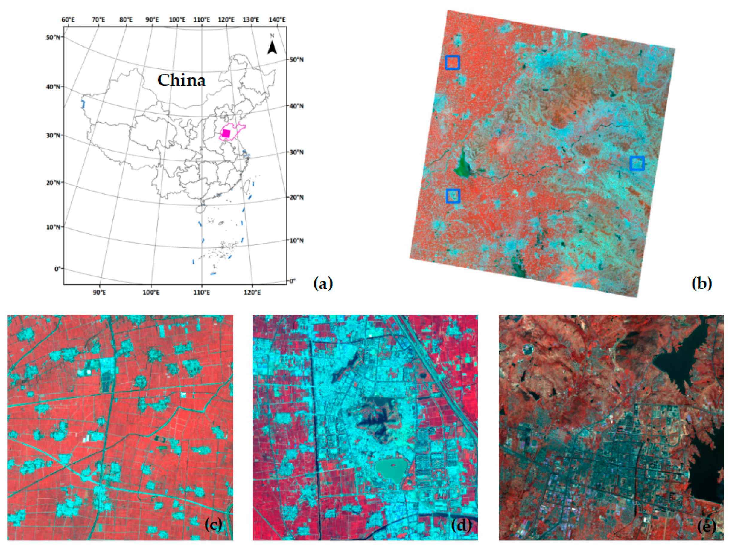
To evaluate the generalization and robustness of the proposed simulation-based unmixing method, a Landsat 8 OLI scene (Path 122/Row 35) in central-western Shandong, China, was selected (Figure 1). The study area features a distinct “urban-rural-natural” gradient, transitioning from expansive alluvial plains to the mountainous terrain of Mount Tai. The region presents significant spectral heterogeneity, including seasonally bare soils and dense metropolitan centers with intricate transportation networks. This complex landscape provides a rigorous testbed to assess the algorithm’s ability to suppress false alarms in non-built-up areas while accurately delineating the geometric details of urban infrastructure against challenging background interference.

2.2. Data Sources and Preprocessing

2.2.1. AVIRIS Imagery and PreProcessing

The Airborne Visible/Infrared Imaging Spectrometer (AVIRIS) project comprises a suite of advanced instruments: AVIRIS Classic (AVIRIS-C), AVIRIS-Next Generation (AVIRIS-NG), and the AVIRIS-3rd Generation (AVIRIS-3). Data derived from these platforms facilitate a broad spectrum of research applications, ranging from terrestrial and coastal aquatic plant physiology, atmospheric and aerosol studies, and environmental science, to snow hydrology, geology, volcanology, oceanography, soil and land management, agriculture, and limnology. Specifically, this study utilizes the AVIRIS-NG Level 2 (L2) Surface Reflectance dataset, as a successor to the classic platform. AVIRIS-NG is a high-fidelity pushbroom spectral mapping system designed with a high signal-to-noise ratio (SNR) for high-performance spectroscopy [29]. The sensor measures upwelling radiance at approximately 5-nm sampling intervals across the entire Visible to Shortwave Infrared (VSWIR) spectral range (380–2510 nm) [30]. With an instantaneous field of view (IFOV) of 1 milliradian, AVIRIS-NG provides altitude-dependent ground sampling distances (GSD) varying from the sub-meter range up to 20 m. To ensure high-precision reference labels for sub-pixel mapping, we specifically selected AVIRIS-NG imagery with a spatial resolution finer than 5 m for this study. The dataset employed in consists of orthocorrected L2 products, which typically include: (a) calibrated surface reflectance, and (b) ancillary data layers such as water vapor and optical absorption paths for liquid water and ice, derived via atmospheric correction algorithms [31].

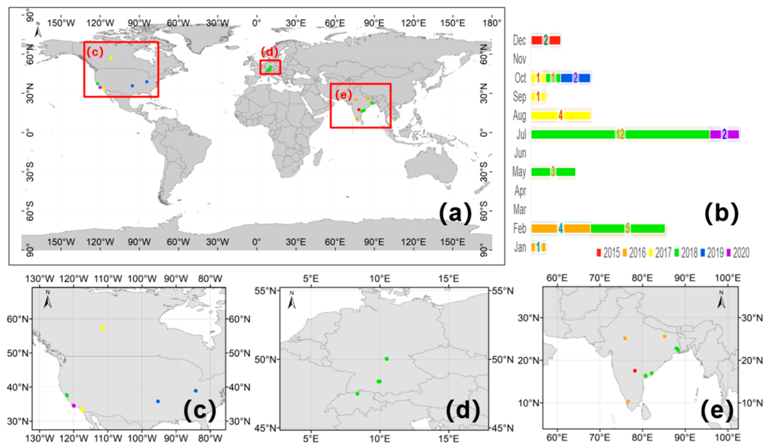
To provide a reliable foundation for subsequent sample construction, we rigorously selected 38 AVIRIS-NG flight lines acquired between 2015 and 2020. These images are spatially and temporally dispersed, maximizing the spectral and spatial heterogeneity across diverse land cover types. A strict quality control protocol was implemented to retain only cloud-free observations with minimal atmospheric interference, ensuring high radiometric accuracy. Furthermore, the selected scenes exhibit distinct land cover features with low ambiguity, effectively avoiding uncertain transition zones. This combination of extensive spatiotemporal coverage and pristine image quality establishes a solid physical basis for generating a high-purity, low-noise sample library. The detailed spatial distribution and temporal coverage of the dataset are illustrated in Figure 2.

To improve the quality of the AVIRIS hyperspectral imagery and ensure the reliability of subsequent analyses, a systematic preprocessing workflow was implemented. First, spectral bands characterized by low signal-to-noise ratios (SNR) or significant atmospheric interference were excluded. This involved the removal of the initial band (Band 1) as well as those located within the water vapor absorption regions, specifically, Bands 195~211 and 281~315. Second, to mitigate inherent spectral noise while preserving the diagnostic absorption features critical for material identification, a Savitzky-Golay (SG) filter was applied to the spectral dimension [32]. Recent studies have validated the efficacy of this method in hyperspectral signal denoising compared to other filtering techniques [33].Finally, a background masking procedure was executed to eliminate invalid pixels (i.e., background artifacts with zero values) from the imagery, ensuring that only the valid study area was retained for the classification model.

2.2.2. Landsat8 OLI Imagery and PreProcessing

To evaluate the effectiveness of the proposed deep learning unmixing framework in real-world scenarios, we selected Landsat 8 Operational Land Imager (OLI) imagery as the target multispectral dataset. We utilized the Landsat 8 Level-2 Science Products (Surface Reflectance) acquired from the U.S. Geological Survey (USGS) Earth Explorer. These products have been atmospherically corrected using the Land Surface Reflectance Code (LaSRC) [34], we selected the six primary optical bands suitable for spectral unmixing: Blue (Band 2), Green (Band 3), Red (Band 4), Near-Infrared (Band 5), and two Shortwave Infrared bands (Band 6 and Band 7). The Coastal Aerosol (Band 1) and Cirrus (Band 9) bands were excluded due to their limited relevance to surface material abundance. The Thermal Infrared bands were also removed, as they cannot be simulated from AVIRIS reflectance data.

2.2.3. High-Resolution Reference (GF-2) and PreProcessing

High-resolution GaoFen-2 (GF-2) imagery with a spatial resolution of 1 m was employed to capture fine-scale ground details and generate reliable reference impervious surface fractions for evaluating Landsat-based sub-pixel unmixing results. A careful mapping and validation procedure was applied to ensure the quality of the reference fractions. These fine-scale maps were subsequently spatially aggregated to 30 m grid cells to match the Landsat resolution, providing accurate validation data for assessing the performance of the inversion models.

3. Methods

This study proposes a hyperspectral simulation-driven framework for sub-pixel impervious surface fraction (ISF) retrieval. The proposed method first constructs a comprehensive target–background spectral library based on hyperspectral observations and generates physically consistent spectrum–abundance training samples through multispectral data simulation. A one-dimensional convolutional neural network (1D-CNN) is then employed to learn the nonlinear relationship between simulated multispectral spectra and ISF values. Finally, a series of comparative experiments are designed to evaluate the effectiveness of the proposed approach using Landsat imagery, and the retrieval performance is assessed through quantitative accuracy metrics and spatial distribution analysis.

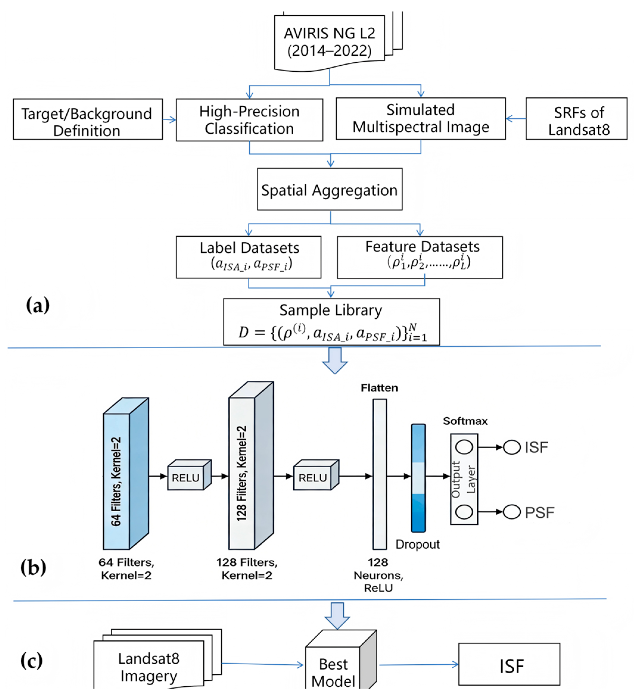
To provide a comprehensive overview of the proposed methodology, we illustrate the end-to-end framework in Figure 3. This framework systematically integrates sample library construction (Section 3.1), 1D-CNN model training (Section 3.2), and the final inference on Landsat imagery.

3.1. Construction of a Comprehensive Target-Background Spectral Library

3.1.1. Definition of Target and Background Endmember Categories

To characterize the inherent complexity of urban surfaces, this study treats Impervious Surface as a single target category rather than dividing it into rigid sub-classes. Based on high-resolution hyperspectral data, we extracted a comprehensive set of spectral features covering a wide dynamic range of anthropogenic materials—from dark asphalt roads to highly reflective metal roofing. Our strategy can be conceptualized as an enhanced, implicit Multiple Endmember Spectral Mixture Analysis (MESMA). While traditional MESMA minimizes reconstruction errors by selecting specific endmembers from a library on a per-pixel basis [11], our framework implicitly encodes the spectral variability of ISA into a massive training dataset derived from hyperspectral simulations. Consequently, the subsequent Convolutional Neural Network (CNN) model learns robust and generalized “ISF features”, which have demonstrated superior performance in capturing non-linear spectral mixing compared to traditional physical models [35,36]. Simultaneously, natural surfaces—including vegetation, soil and water—are defined as pervious surface (PS). By decoupling the target (ISF) from PS, our model ensures accurate estimation of ISF regardless of the surrounding environment. A detailed list of the constituents covering this wide spectral range is provided in

Table 1. The hierarchical composition of the endmember spectral library, categorized into the target IS class and diverse background components.

Endmember Class	Sub-Category	Description
Impervious surface	Building Materials	Rooftops (tile, metal, concrete), industrial structures.
	Transportation	Asphalt roads, paved driveways, parking lots, concrete sidewalks.
Pervious Surface	Vegetation	Natural Vegetation: Forests (deciduous/evergreen), grasslands, tundra, shrubs.
		Artificial Vegetation: Croplands, orchards, pastures, plantations, urban green spaces (lawns).
	Soil	Natural Bare Ground: Rocks, sand, tidal flats, saline-alkali land.
		Agricultural Soil: Fallow fields (unseeded farmland), dry clay.
	Water	Open Water Bodies: Lakes, reservoirs, rivers, streams.
		Other: Saline water, dark deep water.

.

3.1.2. Supervised Classification of Ground Truth Generation

To generate high-precision land-cover maps from high-dimensional AVIRIS imagery, we employed the Support Vector Machine (SVM) classifier. SVM is widely recognized for its superior generalization capability and robustness in handling high-dimensional data with limited training samples, making it particularly well-suited for hyperspectral image classification [15,37]. Comparative studies have consistently demonstrated that SVM outperforms traditional classifiers such as Maximum Likelihood (MLC) and shallow neural networks in complex remote sensing tasks [38].

To optimize classification performance, we implemented a specialized processing workflow. First, the original 372 spectral bands were subjected to Minimum Noise Fraction (MNF) transformation to suppress noise and mitigate spectral redundancy. The first 20 MNF components, which cumulatively account for over 99% of the spectral variance, were selected as input features. The SVM model utilized a Radial Basis Function (RBF) kernel, with the penalty parameter (C) and kernel width (γ) optimized through a grid search strategy combined with 5-fold cross-validation.

Given that the resulting classification maps serve as the foundational “ground truth” for our subsequent deep learning framework, ensuring accurate class consistency is critical. Accordingly, a strict scene-by-scene independent validation approach was employed. To address the complex illumination effects present in high-resolution AVIRIS imagery (including shadows cast by buildings and tree canopies), a “shade” endmember was added to the system originally defined in Section 3.1.1.

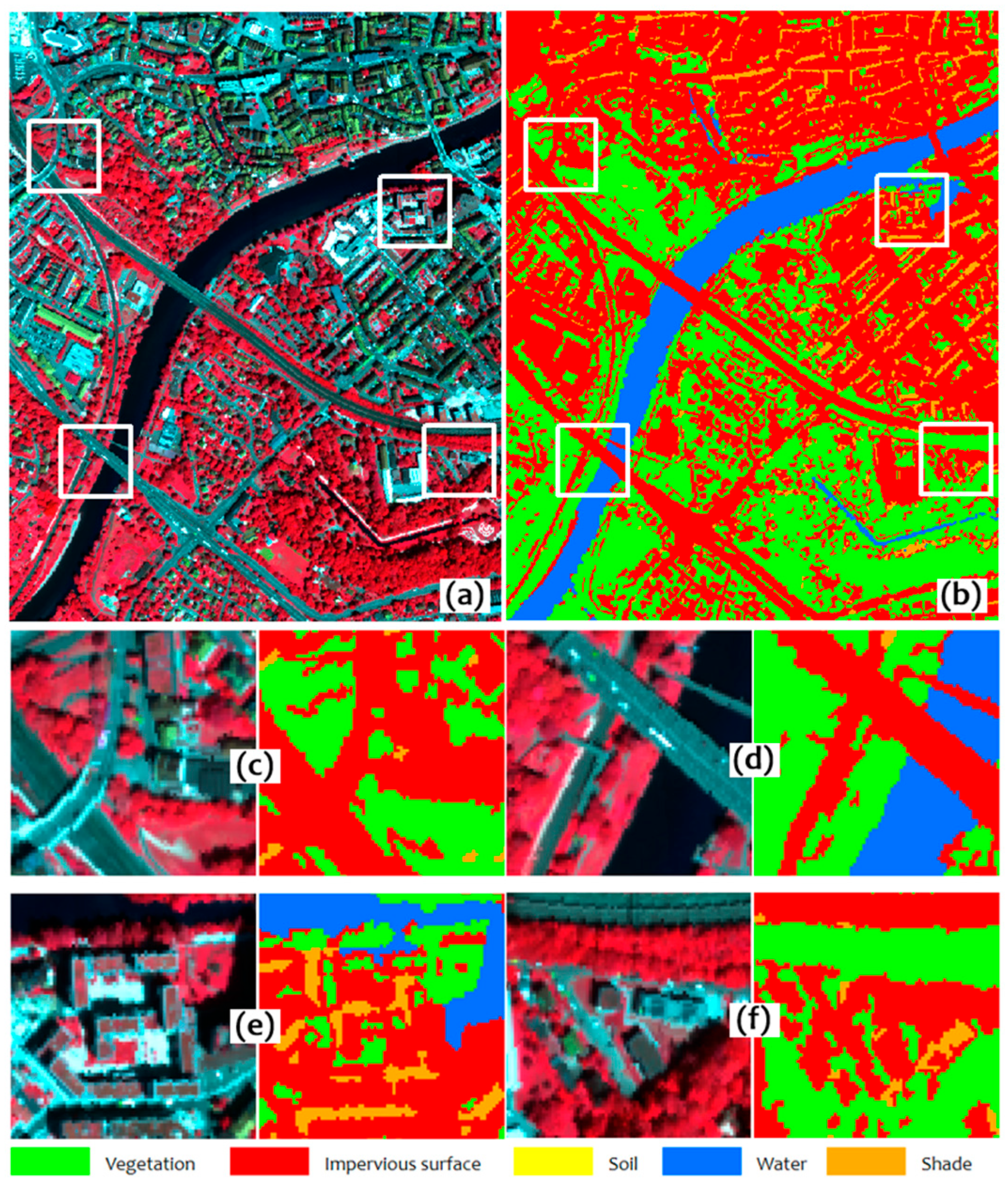
Reference samples (Regions of Interest, ROIs) for the five target categories were manually delineated through visual interpretation of high-resolution RGB composites. To ensure the representativeness and spectral purity of the training samples, a rigorous manual sampling strategy was implemented. ROIs for the five target categories were uniformly distributed across the entire hyperspectral scene to capture the natural intra-class variability under different illumination and background conditions. Furthermore, to minimize edge effects and the risk of mixed pixels, the ROIs were strictly delineated at the central locations of large, continuous, and homogeneous land cover patches, carefully avoiding transition zones and structural boundaries. These highly pure ROIs were utilized exclusively for training the scene-specific SVM classifiers. Finally, each classification result underwent exhaustive manual inspection and iterative refinement to ensure an Impervious Surface (IS) extraction accuracy exceeding 95%. Qualitative assessment of the representative classification results is illustrated in Figure 4.

3.1.3. Multispectral Data Simulation

• Simulation Principle and Implementation

Theoretically, the radiance or reflectance recorded by a multispectral sensor is the weighted integral of the incoming continuous spectrum and the band-specific sensitivity of the sensor. Given that AVIRIS data provides fine-grained spectral information (5 nm sampling) covering the spectral range of most optical satellite sensors, it can be utilized to simulate broad-band multispectral data with high fidelity [39]. To generate the simulated multispectral imagery from the AVIRIS-NG hyperspectral data, we employed the spectral convolution method based on the Spectral Response Functions (SRFs) of the target sensor. Previous studies have validated the physical fidelity of this synthesis approach, demonstrating high radiometric consistency between SRF-synthesized bands and actual multispectral observations [40]. The simulation process, often referred to as spectral resampling or convolution, models the physical response mechanism of the sensor. The formula for data simulation was as follows:

$${\mathrm{L}}_{\mathrm{i}}^{\mathrm{MSI}} = {\displaystyle \frac{\sum _{\mathrm{j}=1}^{{\mathrm{N}}_{\mathrm{HSI}}}{\mathrm{c}}_{\mathrm{ij}}{ {∆}_{\mathrm{j}}\mathrm{L}}_{\mathrm{j}}^{\mathrm{HSI}} }{\sum _{\mathrm{j}=1}^{{\mathrm{N}}_{\mathrm{HSI}}}{\mathrm{c}}_{\mathrm{ij}}{∆}_{\mathrm{j}}}} \mathrm{for} \mathrm{i} =1,\dots , {\mathrm{N}}_{\mathrm{MSI}}$$

(1)

where ${\mathrm{L}}_{\mathrm{i}}^{\mathrm{MSI}}$ is the spectral radiance of the synthesized multispectral image bands, ${ \mathrm{L}}_{\mathrm{j}}^{\mathrm{HSI}}$ is the spectral radiance of the hyperspectral radiances. ${\mathrm{N}}_{\mathrm{MSI}}$ is the band numbers of multispectral instrument (MSI), ${\mathrm{N}}_{\mathrm{HSI}}$ is the band numbers of hyperspectral instrument (HSI), ${∆}_{\mathrm{j}}$ is the channel width of hyperspectral instrument, ${\mathrm{c}}_{\mathrm{ij}}$ is spectral response function of multispectral sensor corresponding to central wavelength of hyperspectral sensor.

In this study, for Landsat 8 OLI, we simulated six spectral bands ranging from the visible to the shortwave infrared (SWIR), encompassing Bands 2 through 7 (Blue, Green, Red, NIR, SWIR-1, and SWIR-2) according to the spectral response functions of Landsat 8 OLI [41]. The high spectral resolution of the source AVIRIS-NG data ensures that a sufficient number of hyperspectral channels fall within the bandwidth of each simulated multispectral band, thereby facilitating accurate weighted integration.

2.

Validation of Simulated Multispectral Imagery

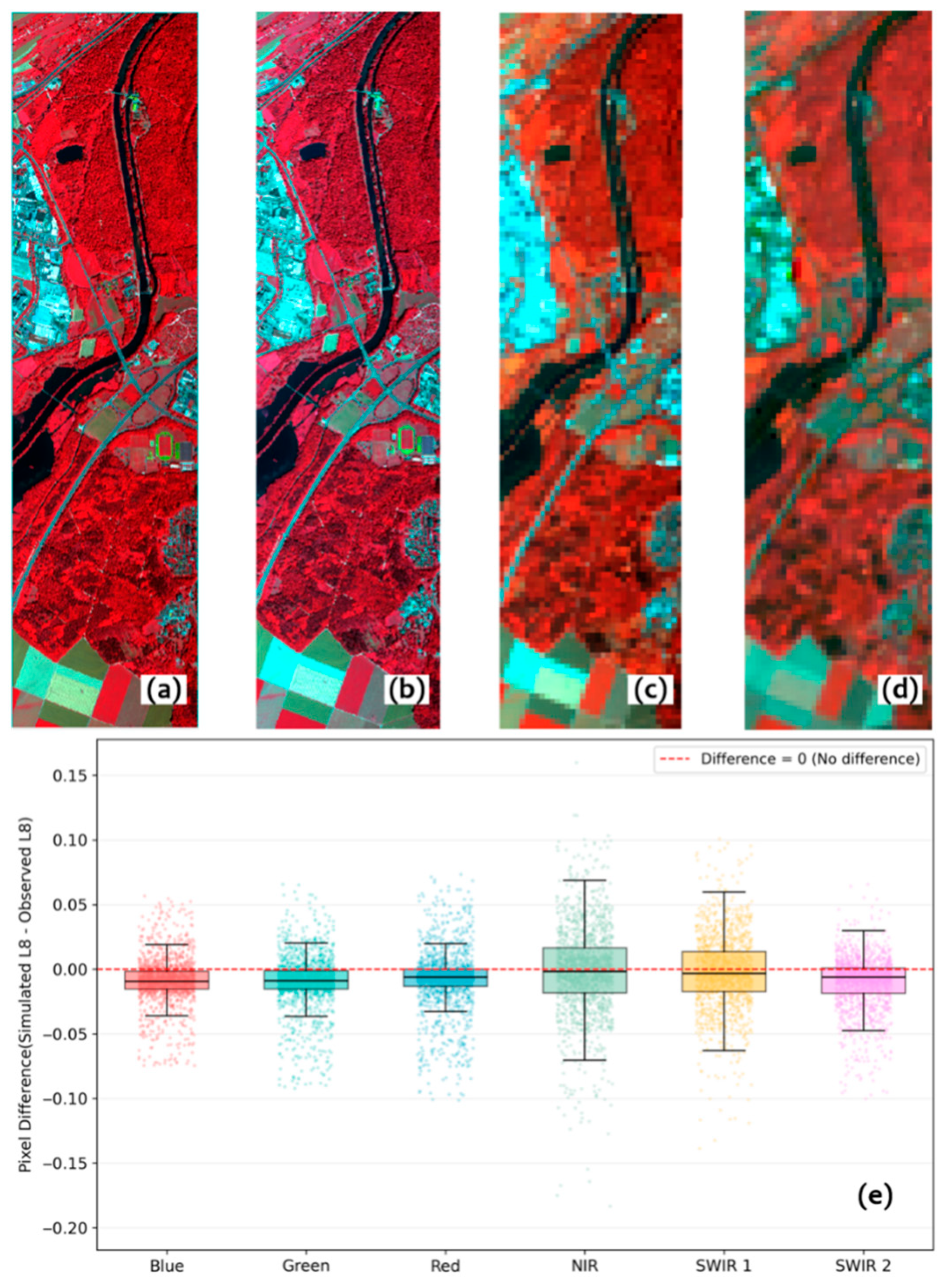
To evaluate the radiometric consistency of the simulation, a comprehensive comparison was performed between the simulated data and actual satellite observations. In principle, the validation imagery should be acquired simultaneously. However, due to cloud cover constraints, we selected the closest available cloud-free Landsat 8 OLI image acquired on 14 July 2018 to validate the AVIRIS-derived simulated image from 2 July 2018. This results in a short 12-day temporal interval.

Visually, Figure 5 demonstrates high consistency between the simulated and observed datasets. The spectral transformation from the hyperspectral domain (Figure 5a) to the broad multispectral bands (Figure 5b) effectively preserved key spectral features. Following spatial aggregation, the simulated 30 m imagery (Figure 5c) exhibited a spatial pattern and radiometric characteristics highly comparable to the actual Landsat 8 image (Figure 5d). Crucially, the boundaries of impervious surfaces (e.g., roads, rooftops) and water bodies remained stable during the 12-day interval, confirming that the simulated data accurately reflects the geometric and radiometric characteristics of the target scene.

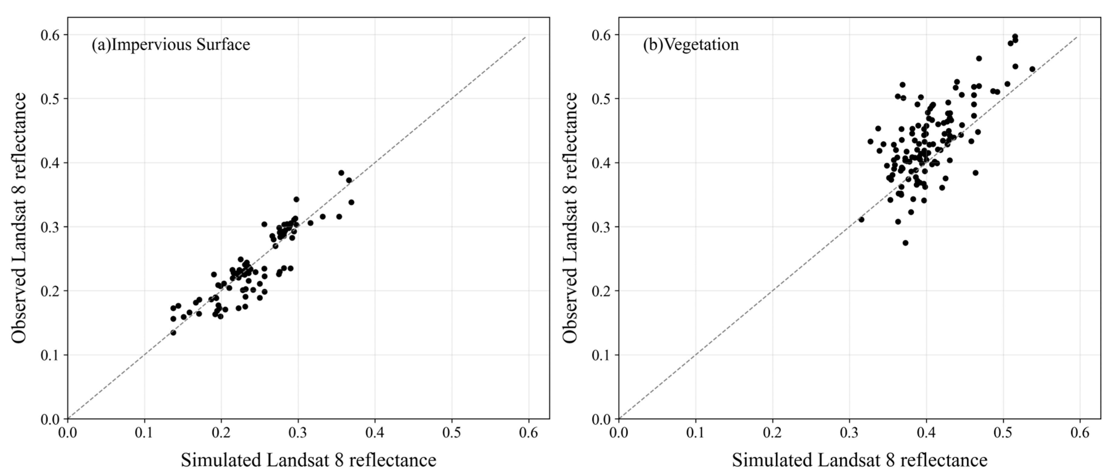
A quantitative pixel-wise difference assessment (Figure 5e) further confirms the spectral consistency between the simulated imagery and the actual Landsat data. The reflectance residuals (Simulated-2 July-Observed 14 July) across all six bands center closely around zero, indicating negligible systematic bias. Specifically, the visible bands (Blue, Green, Red) show extremely tight interquartile ranges. It is worth noting that the NIR and SWIR bands exhibit slightly broader variances compared to the visible bands. To quantitatively assess the uncertainty introduced by this 12-day temporal gap, we evaluated the reflectance bias (simulated minus observed) in the highly phenology-sensitive NIR band. As illustrated by the scatterplots in Figure 6, temporally invariant artificial surfaces show a negligible mean bias of 0.32%, confirming the high fidelity of our spectral simulation. Conversely, vegetation samples exhibit a minor negative bias of −2.84%. This slight deviation aligns with the natural increase in vegetation vigor during early July, demonstrating that the observed variance in the NIR band is fundamentally driven by natural phenological shifts rather than systemic simulation errors.

3.1.4. Construction of the Physically Guided “Spectrum-Abundance” Sample Library

To effectively establish the mapping between spectral signatures and sub-pixel compositions, we constructed a paired endmember sample library $\mathrm{D} ={ \left\{({\mathsf{\rho }}^{\left(\mathrm{i}\right)},{\mathrm{a}}_{\mathrm{I}\mathrm{S}\mathrm{F}\_\mathrm{i}},{\mathrm{a}}_{\mathrm{P}\mathrm{S}\mathrm{F}\_\mathrm{i}})\right\}}_{\mathrm{i}=1}^{\mathrm{N}}$. In this dataset, the input features ${\mathsf{\rho }}^{\left(\mathrm{i}\right)}$ represent the multispectral reflectance, while the labels ${\mathrm{a}}^{\left(\mathrm{i}\right)}$ correspond to the fractional abundances of the endmembers. As illustrated in Figure 3, the abundance vectors $\mathrm{a} = [{\mathrm{a}}_{\mathrm{I}\mathrm{S}\mathrm{F}\_\mathrm{i}},{\mathrm{a}}_{\mathrm{P}\mathrm{S}\mathrm{F}\_\mathrm{i}}]$ and the multispectral reflectance $\mathsf{\rho }\mathsf{ϵ}{\mathrm{R}}^{\mathrm{L}}$ are generated through the following steps. The construction process strictly follows the physical mechanisms of spectral mixing, ensuring that the synthesized data is both statistically diverse and physically realistic.

• Label Generation: Spatial Aggregation from High-Resolution Truth

The abundance labels ${\mathrm{a}}^{\left(\mathrm{i}\right)}$ were derived from high-spatial-resolution hyperspectral imagery (e.g., AVIRIS) to preserve real-world land cover patterns. First, the high-resolution imagery was classified to generate a fine-scale ground truth map. The dimensions of the spatial aggregation window were strictly determined by the resolution relationship between the observed multispectral sensor and the high-resolution source data. Specifically, let $\mathrm{S}$ denote the scaling factor defined by the ratio of the spatial resolution of the multispectral sensor to that of the hyperspectral data. We applied a window of size $\mathrm{S} \times \mathrm{S}$ to traverse the classification map. The classification map was then aggregated using an $\mathrm{S} \times \mathrm{S}$ moving window. The abundance vector for each simulated pixel was then calculated as the areal fraction of each endmember class within this window:

$${\mathrm{a}}_{\mathrm{k}}={\displaystyle \frac{{\mathrm{N}}_{\mathrm{k}}}{{\mathrm{N}}_{\mathrm{total}}}}$$

(2)

where ${\mathrm{N}}_{\mathrm{k}}$ denotes the number of high-resolution pixels belonging to the k-th endmember class, and ${\mathrm{N}}_{\mathrm{total}}$ is the total number of pixels in the aggregation window (i.e., ${\mathrm{N}}_{\mathrm{total}}$= S × S). This method ensures the labels satisfy the abundance non-negativity and sum-to-one constraints naturally while accurately reflecting the scale difference between the sensors.

2.

Feature Generation: Physically Based Spatial Aggregation

Corresponding to the derived abundance labels, the multispectral reflectance features ${\mathsf{\rho }}^{\left(\mathrm{i}\right)}$ were obtained via direct spatial aggregation of the high-resolution imagery. After spectrally resampling the AVIRIS data to Landsat 8 bands using Spectral Response Functions (SRFs), we performed spatial downsampling to match the 30 m resolution. For each coarse-resolution pixel, the reflectance was derived by averaging the reflectance of all spatially aligned high-resolution sub-pixels, ensuring consistency between scales.

The feature vector ${\mathsf{\rho }}^{\left(\mathrm{i}\right)}$ is calculated as:

$${\mathsf{\rho }}^{\left(\mathrm{i}\right)} = {\displaystyle \frac{1}{\mathrm{K}}}\sum _{\mathrm{k}=1}^{\mathrm{K}}{\mathrm{s}}_{\mathrm{k}}$$

(3)

where K is the total count of high-resolution sub-pixels located within the $\text{i-th}$ target multispectral grid, and ${\mathrm{s}}_{\mathrm{k}}$ is the reflectance of the $\text{k-th}$ sub-pixel.

This direct spatial aggregation strategy is widely adopted in remote sensing to generate reliable abundance ground truth and simulation datasets for validating unmixing algorithms [42,43]. Compared to purely mathematical synthesis, this approach preserves the real-world spectral complexity (e.g., intra-class variability) inherent in the high-resolution observations [12], ensuring that the input features $\mathsf{\rho }$ naturally align with the abundance labels derived in the previous step.

Based on the proposed physically constrained spectrum-abundance coupling framework, this study constructed a specialized sample library for urban impervious and pervious surface components. First, land cover types derived from the interpretation of high-spatial-resolution hyperspectral imagery were reclassified into two primary endmembers: impervious surfaces and pervious surfaces. Their sub-pixel abundance fractions at the multispectral pixel scale were then calculated via spatial aggregation. Correspondingly, the multispectral reflectance features were derived through spectral consistency resampling and spatial aggregation of the high-resolution imagery. This construction process not only preserves physically realistic spectral mixing mechanisms and intra-class spectral variability but also achieves physical consistency between spectral features and abundance labels at the spatial scale. Consequently, it provides a robust training sample foundation for the sub-pixel abundance inversion of impervious surfaces and related urban environmental analyses.

3.2. Training of CNN Model

To effectively map the complex non-linear relationship between the simulated medium-resolution spectra and the corresponding Impervious Surface Fraction, a One-Dimensional Convolutional Neural Network (1D-CNN) was employed. Operating directly on individual pixel-wise spectral vectors, the 1D-CNN is highly adept at extracting latent spectral features and capturing local correlations across adjacent spectral bands, making it exceptionally well-suited for pixel-based quantitative inversion tasks. To rigorously assess the model’s generalization capability, we implemented a spatial disjoint partitioning strategy for dataset splitting. Specifically, the sample pool was divided into several independent subsets, each containing approximately 200,000 samples, with 80% randomly assigned for training and 20% for validation. To ensure the reliability of the training library, a strict quality control protocol was applied before splitting to exclude 23,240 anomalous pixels that violated key physical constraints. These constraints required spectral reflectance to remain within the [0, 1] range and the total abundance sum to fall strictly between 0.9998 and 1.0002. Following this optimization, a final dataset of 9,933,359 high-quality samples was obtained.

The specific architecture of the 1D-CNN is illustrated in Figure 6. It consists of two convolutional layers with 64 and 128 filters, respectively, utilizing a kernel size of 2. To preserve fine-scale spectral signatures, pooling layers were omitted, and ReLU activation functions were applied throughout to capture non-linear features. The extracted feature vectors are flattened and passed through a 128-neuron fully connected layer, which incorporates a Dropout layer to mitigate overfitting across the large sample pool. Finally, a Softmax activation is utilized in the output layer to enforce the sum-to-one constraint, ensuring that the predicted abundances are physically realistic.

Training was conducted with a batch size of 128 and an initial learning rate of 0.001 using the Adam optimizer. While the maximum number of epochs was set to 100, an early stopping mechanism was implemented to monitor validation Mean Absolute Error (MAE), terminating the process if no improvement occurred for 10 consecutive rounds.

3.3. Experimental Design

To systematically evaluate the performance of the proposed sample generation strategy and the 1D-CNN unmixing model, three comparative experimental schemes were designed

Table 2. Summary of the experimental design.

Experiment ID	Training Data Source	Unmixing Model	Objective
Experiment 1 (Exp.1)	Image-derived (Landsat)	Random Forest (RF)	Baseline comparison (Traditional method)
Experiment 2 (Exp.2)	Simulated (Hyperspectral)	Random Forest (RF)	Validate the sample generation strategy
Experiment 3 (Exp.3)	Simulated (Hyperspectral)	1D-CNN	Validate the model architecture (Proposed)

. These experiments function as an ablation study to isolate the contributions of the high-quality training data and the deep learning architecture, respectively. Experiment 1 serves as the traditional baseline, where training samples were manually selected directly from the Landsat 8 imagery based on visual interpretation, and the Random Forest (RF) regressor was employed for unmixing. To validate the effectiveness of the data generation strategy, Experiment 2 utilized the hyperspectral-simulated sample library (constructed in Section 3.1) as the training data, while keeping the unmixing model (RF) unchanged. A comparison between Experiment 1 and Experiment 2 allows for quantifying the impact of sample quality—specifically spectral purity and intra-class variability—on unmixing accuracy. Finally, Experiment 3 represents the complete methodology proposed in this study, which integrates the hyperspectral-simulated library with the 1D-CNN model (described in Section 3.2). By comparing Experiment 2 and Experiment 3, where the training data remains identical, the superiority of the 1D-CNN architecture over traditional machine learning in extracting non-linear spectral features can be explicitly demonstrated. All data preprocessing, model training, and result analysis in this study were performed using open-source software and general-purpose computing hardware. Specifically, the core algorithms were implemented in Python 3.11.5, with key open-source libraries including NumPy, Pandas, Scikit-learn, TensorFlow 2.15.0, Rasterio, and GDAL.

3.4. Accuracy Assessment

3.4.1. Accuracy Evaluation Metrics

To quantitatively evaluate the performance of the proposed method in estimating subpixel endmember fractions, we employed three standard statistical metrics: Root Mean Square Error (RMSE), Mean Absolute Error (MAE), and the Coefficient of Determination (${\mathrm{R}}^2$). RMSE serves as the primary indicator of the overall deviation, giving greater weight to larger errors to reflect model robustness, while MAE provides a direct measurement of the average absolute difference between the estimated and ground-truth values, representing the physical accuracy of the unmixing results. Additionally, ${\mathrm{R}}^2$ is utilized to assess the goodness of fit and the proportion of variance explained by the model. These metrics are mathematically defined as:

$$\mathrm{RMSE} =\sqrt{{\displaystyle \frac{1}{\mathrm{N}}}{\sum }_{\mathrm{i}=1}^{\mathrm{N}}{({\hat{\mathrm{a}}}_{\mathrm{i}}-{\mathrm{a}}_{\mathrm{i}})}^2}$$

(4)

$$\mathrm{MAE}={\displaystyle \frac{1}{\mathrm{N}}}{\sum }_{\mathrm{i}=1}^{\mathrm{N}}\left|{\hat{\mathrm{a}}}_{\mathrm{i}}-{\mathrm{a}}_{\mathrm{i}}\right|$$

(5)

$${\mathrm{R}}^2=1-{\displaystyle \frac{{\sum }_{\mathrm{i}=1}^{\mathrm{N}}{({\mathrm{a}}_{\mathrm{i}}-{\hat{\mathrm{a}}}_{\mathrm{i}})}^2}{{\sum }_{\mathrm{i}=1}^{\mathrm{N}}{({\mathrm{a}}_{\mathrm{i}}-{\stackrel{\mathrm{-}}{\mathrm{a}}}_{\mathrm{i}})}^2}}$$

(6)

where N denotes the total number of samples, ${\mathrm{a}}_{\mathrm{i}}$ and ${\hat{\mathrm{a}}}_{\mathrm{i}}$ represent the actual and estimated abundance fractions for the i-th sample, respectively, and ${\stackrel{\mathrm{-}}{\mathrm{a}}}_{\mathrm{i}}$ corresponds to the mean of the observed abundances [27,44]. Consequently, lower RMSE and MAE values, combined with an ${\mathrm{R}}^2$ value approaching 1, demonstrate superior unmixing accuracy and generalization capability.

3.4.2. Validation Data

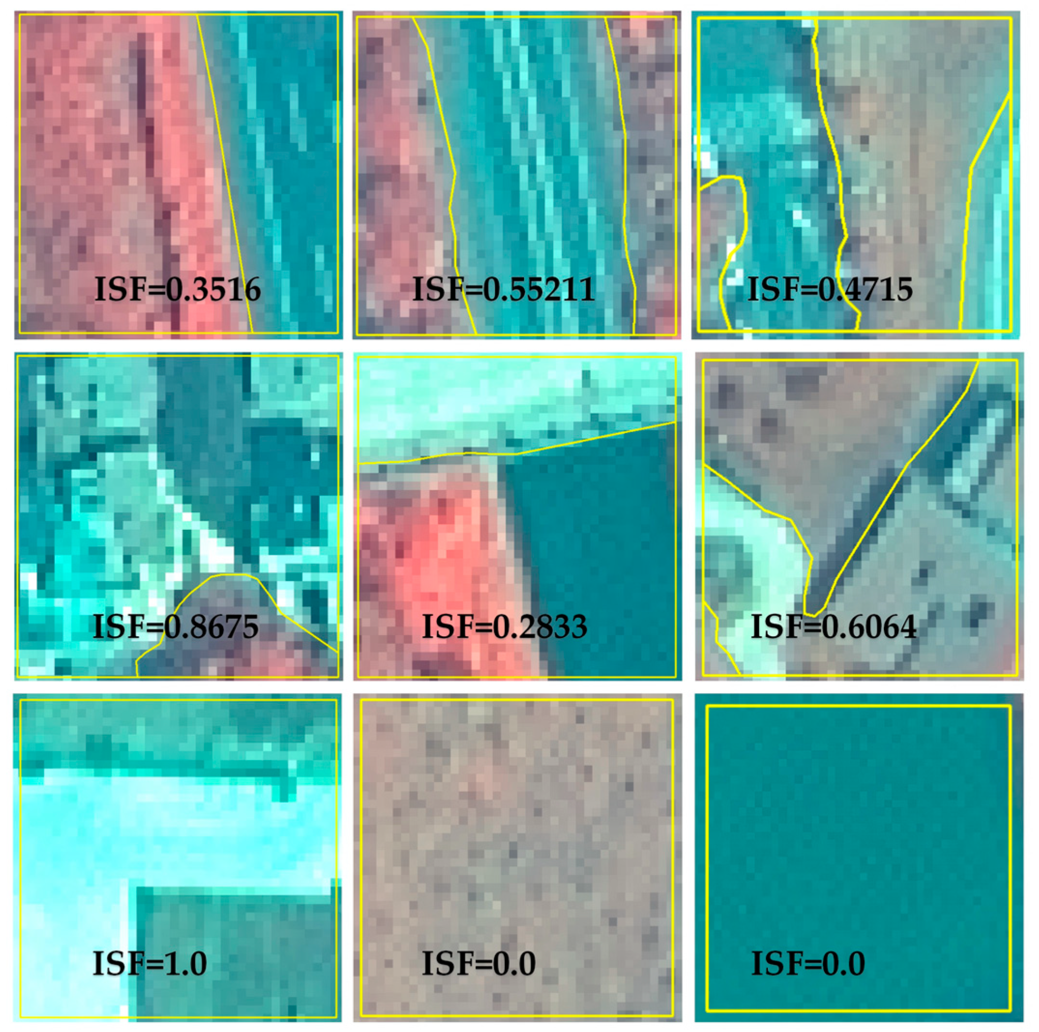
To evaluate the mode’s performance using real observations, an independent validation set containing 4259 samples was manually labeled from high-resolution GaoFen-2 (GF-2) imagery with a spatial resolution of 1 m. This external dataset is completely independent of the simulated training data. As shown in Figure 7, high-resolution impervious surface features were first vectorized from GF-2 images and then aggregated into 30 m grid cells to be consistent with the spatial resolution of Landsat 8. Each validation sample represents the actual Impervious Surface Fraction (ISF) within a 30 m pixel, providing reliable ground truth for evaluating inversion accuracy in real urban and rural scenarios.

4. Results

4.1. Quantitative Assessment

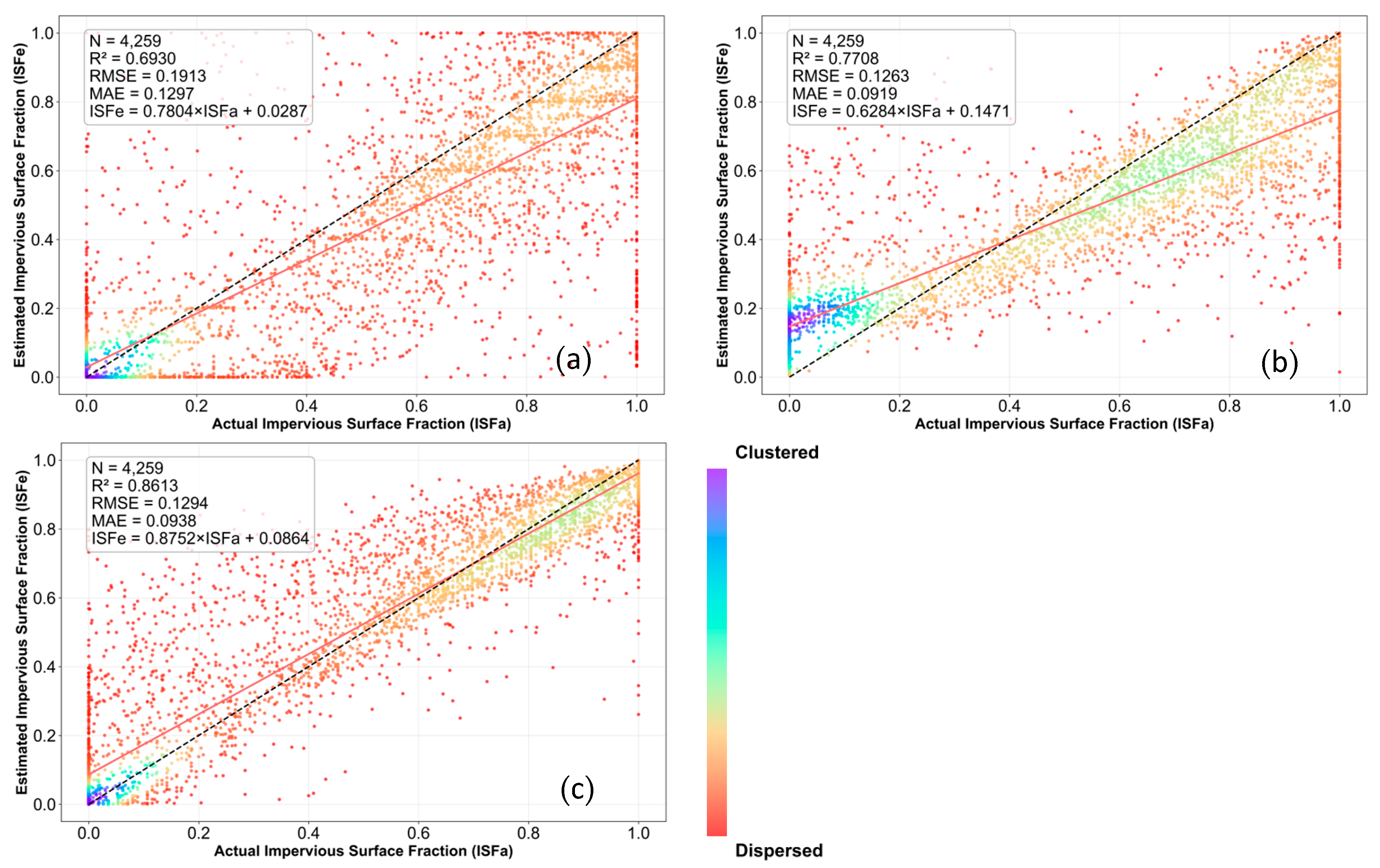
To systematically evaluate the proposed unmixing framework, three experimental schemes were compared using 4259 validation samples. As shown in

Table 3. Quantitative comparison of unmixing accuracy metrics among three experimental schemes across the overall study area and specific sub-regions (refer to Figure 1 for sub-region delineation).

Region	Method	${\mathbf{R}}^2$	RMSE	MAE	Slope	Intercept
Overall	Exp.1	0.6930	0.1913	0.1297	0.7804	0.0287
	Exp.2	0.7708	0.1263	0.0919	0.6284	0.1471
	Exp.3	0.8613	0.1294	0.0938	0.8752	0.0864
Rural (Site c)	Exp.1	0.7937	0.1526	0.0889	0.8289	0.0016
	Exp.2	0.8495	0.0872	0.0640	0.5737	0.1326
	Exp.3	0.9409	0.0811	0.0476	0.8953	0.0208
Urban (Site d)	Exp.1	0.6632	0.1796	0.1217	0.7535	0.0792
	Exp.2	0.7214	0.1356	0.1009	0.6524	0.1914
	Exp.3	0.7578	0.1189	0.0822	0.6286	0.3415
mountain-urban transition (Site e)	Exp.1	0.6982	0.1844	0.1260	0.7414	0.1097
	Exp.2	0.7193	0.1530	0.1134	0.6475	0.1561
	Exp.3	0.8649	0.1295	0.0996	0.8661	0.1160

and the corresponding scatterplots in Figure 8, accuracy improved step-wise from Exp.1 to Exp.3. Exp.1 (image-derived samples + RF) had the lowest accuracy (RMSE = 0.1913, ${\mathrm{R}}^2$ = 0.6930) with dispersed scatter points and outliers due to sample label noise. Exp.2 (hyperspectral-simulated samples + RF) significantly improved performance (RMSE = 0.1263, ${\mathrm{R}}^2$ = 0.7708), verifying the simulated library’s ability to reduce random errors, but a saturation effect remained (slope = 0.6284). Exp.3 (simulated samples + 1D-CNN) achieved the most robust performance: though RMSE (0.1294) was similar to Exp.2, it corrected systematic bias (slope = 0.8752, ${\mathrm{R}}^2$ = 0.8613), with scatter points converging along the 1:1 line. Regional analysis showed superiority across diverse zones in Exp.3: it suppressed noise in Site c (rural agriculture, ${\mathrm{R}}^2$ = 0.9409), achieved the lowest RMSE (0.1189) in Site d (urban core), and corrected saturation in Site e (mountain-urban transition, slope = 0.8661). Overall, combining the hyperspectral-simulated library and 1D-CNN provides a generalized, robust solution for regional ISF mapping.

4.2. Spatial Distribution and Visual Comparison

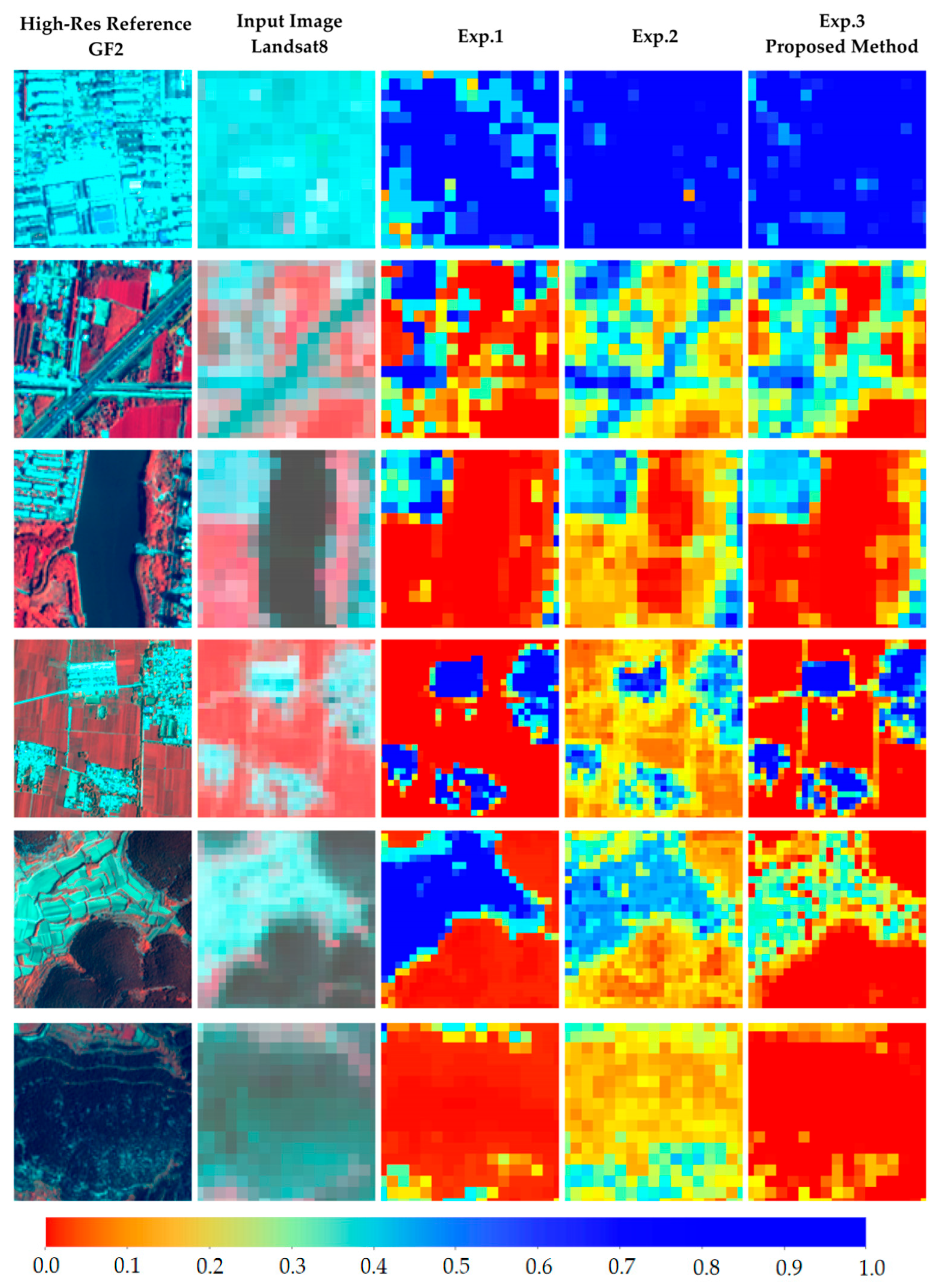
To qualitatively evaluate the spatial details and boundary preservation of the estimated impervious surface fraction (ISF), three methods were visually compared in six representative landscape subsets (Figure 9). The high-resolution GF-2 images are used as ground-truth references, while the low-resolution Landsat-8 images serve as the model inputs. The color bar indicates the ISF, ranging from 0 (red, representing pure pervious surfaces like vegetation, water, and bare soil) to 1 (blue, representing pure impervious surfaces like dense buildings).

As observed in Figure 9, the three experiments exhibit significant differences in spatial characterization. Exp.1 demonstrates a severe polarization effect, struggling significantly with false positives in non-urban regions. For instance, in complex backgrounds such as agricultural lands and mountainous areas (rows 4 and 5), Exp.1 erroneously generates large contiguous patches of high ISF values (dark blue), indicating its poor capability in distinguishing bare soil from impervious surfaces. Conversely, Exp.2 suffers from a pronounced over-smoothing phenomenon and a “regression-to-the-mean” tendency. It fails to capture extreme ISF values accurately, systematically overestimating low-abundance areas—yielding yellow or green pixels in completely natural terrains (rows 5 and 6)—while underestimating high-density urban cores (row 1). Consequently, the geometric boundaries of linear features, such as highways and riverbanks (rows 2 and 3), are severely blurred in the Exp.2 results. In contrast, the Proposed Method (Exp.3) achieves the highest visual fidelity and spatial consistency with the high-resolution reference imagery. It effectively suppresses background noise, successfully outputting pure pervious estimations (red) in mountainous areas and water bodies without interference. Furthermore, Exp.3 accurately preserves the fine spatial details and geometric boundaries of scattered rural settlements and narrow roads (rows 2 and 4), successfully mitigating both the severe false-positive issue of Exp.1 and the blurring effect of Exp.2. Overall, the visual assessment confirms that the proposed method possesses superior robustness against complex backgrounds and provides a more accurate and realistic spatial distribution of ISF.

5. Discussion

5.1. Effectiveness of the Simulation-Based Training Dataset

The proposed hyperspectral simulation-driven framework demonstrates superior efficacy in Impervious Surface Fraction (ISF) retrieval. By integrating high-resolution airborne hyperspectral data, spectral convolution, and spatial aggregation, this approach constructs a training dataset characterized by rigorous physical consistency. Unlike conventional methods that rely on manually interpreted samples—often subject to by geometric misregistration, temporal inconsistencies, and subjective labeling errors—our framework ensures a strict correspondence between spectral features and abundance labels. This simulation-based generation mitigates data uncertainty by deriving both reflectance and ground truth from a unified, high-fidelity hyperspectral source. Consequently, the model benefits from more reliable supervision, leading to enhanced retrieval accuracy, improved preservation of spatial boundaries, and a significant reduction in false alarms within non-urban regions. These findings confirm that our physically constrained training library effectively captures the spectral characteristics of impervious surfaces, thereby substantially improving the stability and robustness of ISF mapping.

5.2. Analysis of Underestimation and Overestimation in ISF Retrieval

Despite overall performance improvements, the quantitative results in dense urban cores (e.g., Site d, slope = 0.6286) indicate a pronounced “regression-to-the-mean” bias, characterized by the systematic underestimation of high ISF values and overestimation of low ISF values. This phenomenon is primarily driven by two complex factors.

First, there is an inherent training sample imbalance heavily skewed toward intermediate ISF values. During the spatial aggregation process from high-resolution imagery to the 30 m Landsat scale, pure pixels (i.e., near 100% or 0% imperviousness) become exceedingly rare due to the high fragmentation of urban landscapes. Consequently, the statistical distribution of the simulated training library assumes a bell shape. Without explicit balancing constraints, the 1D-CNN optimizes its overall loss by adopting conservative predictions biased toward this central tendency, inevitably suppressing extreme high values.

Second, the underperformance is exacerbated by nonlinear spectral mixing effects prevalent in dense built-up areas. The current simulation pipeline generates multi-spectral features based on a linear spatial aggregation assumption (Equation (3)). However, dense urban cores feature complex 3D geometric structures, including tall buildings and narrow street canyons, which induce severe multiple scattering and deep shadowing effects. The linear synthesis fails to fully replicate these complex 3D radiative transfer mechanisms, leading to a physical discrepancy between the simulated training spectra and the actual multispectral observations recorded by the satellite.

5.3. Theoretical Potential for Cross-Sensor Extension

A distinctive feature of the proposed simulation-driven framework is its independence from specific sensor configurations, as it relies on high-resolution airborne hyperspectral imagery as a unified spectral information source. In principle, the framework generates sensor-specific training datasets through spectral convolution with the Spectral Response Functions (SRFs) of the target platform. This mechanism suggests a high potential for extending the methodology to other medium-resolution satellites, such as Sentinel-2 or MODIS, simply by substituting the SRF profile of the target sensor.

While our current validation is focused on Landsat 8 imagery, the modular design of this simulation-based approach provides a flexible paradigm for future cross-sensor model migration, potentially bypassing the labor-intensive requirements of manual re-labeling for different platforms. We acknowledge that the empirical robustness of this adaptability remains to be fully verified. Future research will incorporate multi-source satellite datasets to validate the universality of this framework across diverse satellite constellations, thereby providing a more systematic solution for long-term, multi-sensor urban environmental monitoring.

5.4. Limitations and Future Work

Despite its promising performance, several limitations of the proposed framework should be acknowledged. First, the construction of the spectral library assumes that hyperspectral pixels represent relatively pure surface materials. This assumption is generally reasonable when the spatial resolution of hyperspectral imagery is sufficiently high (e.g., finer than approximately 5 m), but mixed pixels may still exist in complex urban environments, which could introduce uncertainty into the spectral library. Second, the proposed framework relies on the availability of high-quality hyperspectral data for sample generation. Although airborne hyperspectral datasets such as AVIRIS provide rich spectral information, their spatial coverage is often limited, which may restrict the large-scale application of the framework. Finally, the current implementation primarily assumes linear spectral mixing during the spatial aggregation process. Incorporating nonlinear spectral mixing models may further improve the realism of simulated spectra and enhance ISF retrieval accuracy in complex urban environments.

To mitigate these limitations in future research, concrete strategies must be implemented at both the data and model levels. To counteract sample imbalance, advanced loss functions—such as focal loss or inverse frequency weighting—should be employed to heavily penalize prediction errors on minority pure pixels during network training. Furthermore, to address nonlinear mixing, future simulation frameworks should incorporate 3D urban canopy models or nonlinear radiative transfer approximations to synthesize more physically realistic training spectra for high-density urban zones.

Future research will focus on expanding the hyperspectral spectral library using datasets from multiple geographic regions, exploring nonlinear spectral mixing mechanisms, and validating the framework across multiple satellite sensors. These efforts will further improve the robustness and scalability of the proposed approach for large-scale impervious surface monitoring.

6. Conclusions

This study addresses the challenge of generating reliable training samples for impervious surface fraction (ISF) mapping from medium-resolution imagery by developing a physically consistent framework based on high-spatial-resolution hyperspectral data. Conventional training samples derived often suffer from geometric misregistration, temporal inconsistencies, and radiometric discrepancies, which limit the accuracy and reliability of ISF inversion models.

Experimental results demonstrate that the proposed approach significantly improves ISF estimation accuracy compared with conventional sample construction strategies. The method effectively suppresses spectral confusion in non-urban areas, restores the natural bimodal distribution of ISF values, and preserves fine spatial boundaries, achieving the highest overall accuracy (R² = 0.8613).

Furthermore, the framework exhibits strong cross-sensor adaptability. By convolving hyperspectral data with the spectral response functions of different sensors, the method can generate sensor-consistent training datasets for platforms such as Landsat and MODIS. This capability significantly reduces the reliance on manual re-labeling when migrating models across sensors, thereby providing a scalable and systematic solution for multi-sensor urban monitoring and long-term impervious surface mapping.

References

1. Arnold, C.L., Jr.; Gibbons, C.J. Impervious Surface Coverage: The Emergence of a Key Environmental Indicator. J. Am. Plan. Assoc. 1996, 62, 243–258. [Google Scholar] [CrossRef]
2. Weng, Q.; Lu, D.; Schubring, J. Estimation of land surface temperature-vegetation abundance relationship for urban heat island studies. Remote Sens. Environ. 2004, 89, 467–483. [Google Scholar] [CrossRef]
3. Zheng, Z.; Pang, B.; Ren, H.; Chen, H.; Zhou, S. Impacts of impervious surface spatial patterns on surface heat island intensity in Chinese cities. J. Beijing Norm. Univ. 2024, 60, 641–650. [Google Scholar] [CrossRef]
4. Gong, P.; Li, X.; Wang, J.; Bai, Y.; Chen, B.; Hu, T.; Liu, X.; Xu, B.; Yang, J.; Zhang, W.; et al. Annual maps of global artificial impervious area (GAIA) between 1985 and 2018. Remote Sens. Environ. 2020, 236, 111510. [Google Scholar] [CrossRef]
5. Wulder, M.A.; White, J.C.; Loveland, T.R.; Woodcock, C.E.; Belward, A.S.; Cohen, W.B.; Fosnight, E.A.; Shaw, J.; Masek, J.G.; Roy, D.P. The global Landsat archive: Status, consolidation, and direction. Remote Sens. Environ. 2016, 185, 271–283. [Google Scholar] [CrossRef]
6. Deng, C.; Zhu, Z. Continuous subpixel monitoring of urban impervious surface using Landsat time series. Remote Sens. Environ. 2020, 238, 110929. [Google Scholar] [CrossRef]
7. Ridd, M.K. Exploring a V-I-S (Vegetation-Impervious Surface-Soil) Model for Urban Ecosystem Analysis Through Remote Sensing. Int. J. Remote Sens. 1995, 16, 2165–2185. [Google Scholar] [CrossRef]
8. Wu, C.; Murray, A.T. Estimating impervious surface distribution by spectral mixture analysis. Remote Sens. Environ. 2003, 84, 493–505. [Google Scholar] [CrossRef]
9. Schug, F.; Frantz, D.; Okujeni, A.; van der Linden, S.; Hostert, P. Mapping urban-rural gradients of settlements and vegetation at national scale using Sentinel-2 spectral-temporal metrics and regression-based unmixing with synthetic training data. Remote Sens. Environ. 2020, 246, 111810. [Google Scholar] [CrossRef]
10. Wu, C. Normalized spectral mixture analysis for monitoring urban composition using ETM+ imagery. Remote Sens. Environ. 2004, 93, 480–492. [Google Scholar] [CrossRef]
11. Roberts, D.A.; Gardner, M.; Church, R.; Ustin, S.; Scheer, G.; Green, R.O. Mapping Chaparral in the Santa Monica Mountains Using Multiple Endmember Spectral Mixture Models. Remote Sens. Environ. 1998, 65, 267–279. [Google Scholar] [CrossRef]
12. Somers, B.; Asner, G.P.; Tits, L.; Coppin, P. Endmember variability in Spectral Mixture Analysis: A review. Remote Sens. Environ. 2011, 115, 1603–1616. [Google Scholar] [CrossRef]
13. Wang, J.; Wu, Z.; Wu, C.; Cao, Z.; Fan, W.; Tarolli, P. Improving impervious surface estimation: An integrated method of classification and regression trees (CART) and linear spectral mixture analysis (LSMA) based on error analysis. GISci. Remote Sens. 2018, 55, 583–603. [Google Scholar] [CrossRef]
14. He, S.; Zhu, L.; Li, Y.; Xia, Q.; Zheng, Q.; Wang, Z.; Zou, X. A comparative analysis of machine learning-based methods for impervious surface mapping using SAR and optical data. Geocarto Int. 2025, 40, 2521833. [Google Scholar] [CrossRef]
15. Mountrakis, G.; Im, J.; Ogole, C. Support vector machines in remote sensing: A review. ISPRS J. Photogramm. Remote Sens. 2011, 66, 247–259. [Google Scholar] [CrossRef]
16. Perikamana, K.K.; Balakrishnan, K.; Tripathy, P. A CNN based method for Sub-pixel Urban Land Cover Classification using Landsat-5 TM and Resourcesat-1 LISS-IV Imagery. arXiv 2021, arXiv:2112.08841. [Google Scholar]
17. Rawat, A.; Gupta, P.; Persello, C. Deep Learning for Built-Up Fractional Mapping Using Sentinel-2 Images: A Case Study in Delhi, India. 2024. Available online: https://www.preprints.org/manuscript/202401.1879 (accessed on 10 March 2024).
18. Wang, J.; Jin, W.; Cao, Z.; Pan, Z.; Yang, G.; Zhao, Y. Improving subpixel impervious surface estimation based on point of interest (POI) data. Int. J. Appl. Earth Obs. Geoinf. 2025, 139, 104538. [Google Scholar] [CrossRef]
19. Maxwell, A.E.; Warner, T.A.; Fang, F. Implementation of machine-learning classification in remote sensing: An applied review. Int. J. Remote Sens. 2018, 39, 2784–2817. [Google Scholar] [CrossRef]
20. Foody, G.M.; Mathur, A. A relative evaluation of multiclass image classification by support vector machines. IEEE Trans. Geosci. Remote Sens. 2004, 42, 1335–1343. [Google Scholar] [CrossRef]
21. Liu, Y.; Wu, Y.; Chen, Z.; Huang, M.; Du, W.; Chen, N.; Xiao, C. A Novel Impervious Surface Extraction Method Based on Automatically Generating Training Samples From Multisource Remote Sensing Products: A Case Study of Wuhan City, China. IEEE J. Sel. Top. Appl. Earth Obs. Remote Sens. 2022, 15, 6766–6780. [Google Scholar] [CrossRef]
22. Tuia, D.; Marcos, D.; Camps-Valls, G. Multi-temporal and multi-source remote sensing image classification by nonlinear relative normalization. ISPRS J. Photogramm. Remote Sens. 2016, 120, 1–12. [Google Scholar] [CrossRef]
23. Schroeder, T.A.; Cohen, W.B.; Song, C.; Canty, M.J.; Yang, Z. Radiometric correction of multi-temporal Landsat data for characterization of early successional forest patterns in western Oregon. Remote Sens. Environ. 2006, 103, 16–26. [Google Scholar] [CrossRef]
24. Miao, J.; Li, S.; Bai, X.; Gan, W.; Wu, J.; Li, X. RS-NormGAN: Enhancing change detection of multi-temporal optical remote sensing images through effective radiometric normalization. ISPRS J. Photogramm. Remote Sens. 2025, 221, 324–346. [Google Scholar] [CrossRef]
25. Demir, B. Learning from Noisy Labels in Remote Sensing. In Proceedings of the AGU Fall Meeting Abstracts, Chicago, IL, USA, 1 December 2022; p. IN33A-02. [Google Scholar]
26. Okujeni, A.; Van der Linden, S.; Jakimow, B.; Rabe, A.; Verrelst, J.; Hostert, P. A Comparison of Advanced Regression Algorithms for Quantifying Urban Land Cover. Remote Sens. 2014, 6, 6324–6346. [Google Scholar] [CrossRef]
27. Bioucas-Dias, J.M.; Plaza, A.; Dobigeon, N.; Parente, M.; Du, Q.; Gader, P.; Chanussot, J. Hyperspectral Unmixing Overview: Geometrical, Statistical, and Sparse Regression-Based Approaches. IEEE J. Sel. Top. Appl. Earth Obs. Remote Sens. 2012, 5, 354–379. [Google Scholar] [CrossRef]
28. Heylen, R.; Parente, M.; Gader, P. A Review of Nonlinear Hyperspectral Unmixing Methods. IEEE J. Sel. Top. Appl. Earth Obs. Remote Sens. 2014, 7, 1844–1868. [Google Scholar] [CrossRef]
29. Hamlin, L.; Green, R.O.; Mouroulis, P.; Eastwood, M.; Wilson, D.; Dudik, M.; Paine, C. Imaging spectrometer science measurements for Terrestrial Ecology: AVIRIS and new developments. In Proceedings of the 2011 Aerospace Conference, Big Sky, MT, USA, 5–12 March 2011; pp. 1–7. [Google Scholar]
30. Chapman, J.W.; Thompson, D.R.; Helmlinger, M.C.; Bue, B.D.; Green, R.O.; Eastwood, M.L.; Geier, S.; Olson-Duvall, W.; Lundeen, S.R. Spectral and Radiometric Calibration of the Next Generation Airborne Visible Infrared Spectrometer (AVIRIS-NG). Remote Sens. 2019, 11, 2129. [Google Scholar] [CrossRef]
31. Thompson, D.R.; Natraj, V.; Green, R.O.; Helmlinger, M.C.; Gao, B.-C.; Eastwood, M.L. Optimal estimation for imaging spectrometer atmospheric correction. Remote Sens. Environ. 2018, 216, 355–373. [Google Scholar] [CrossRef]
32. Savitzky, A.; Golay, M. Smoothing and Differentiation of Data by Simplified Least Squares Procedures. Anal. Chem. 1964, 36, 1627–1639. [Google Scholar] [CrossRef]
33. Ibrahim, I.; AlRowaily, M.H.; Arof, H.; Abu Talip, M.S. Performance Comparison of Selected Filters in Fast Denoising of Oil Palm Hyperspectral Data. Appl. Sci. 2024, 14, 8895. [Google Scholar] [CrossRef]
34. Vermote, E.; Justice, C.; Claverie, M.; Franch, B. Preliminary analysis of the performance of the Landsat 8/OLI land surface reflectance product. Remote Sens. Environ. 2016, 185, 46–56. [Google Scholar] [CrossRef]
35. Lin, C.-H.; Wang, T.-Y. A novel convolutional neural network architecture of multispectral remote sensing images for automatic material classification. Signal Process. Image Commun. 2021, 97, 116329. [Google Scholar] [CrossRef]
36. Mou, L.; Bruzzone, L.; Zhu, X.X. Learning Spectral-Spatial-Temporal Features via a Recurrent Convolutional Neural Network for Change Detection in Multispectral Imagery. IEEE Trans. Geosci. Remote Sens. 2019, 57, 924–935. [Google Scholar] [CrossRef]
37. Melgani, F.; Bruzzone, L. Classification of hyperspectral remote sensing images with support vector machines. IEEE Trans. Geosci. Remote Sens. 2004, 42, 1778–1790. [Google Scholar] [CrossRef]
38. Huang, C.; Davis, L.S.; Townshend, J.R.G. An assessment of support vector machines for land cover classification. Int. J. Remote Sens. 2002, 23, 725–749. [Google Scholar] [CrossRef]
39. Green, R.O.; Shimada, M. On-orbit calibration of a multi-spectral satellite sensor using a high altitude airborne imaging spectrometer. Adv. Space Res. 1997, 19, 1387–1398. [Google Scholar] [CrossRef]
40. Blonksi, S.; Gasser, G.; Russell, J.; Ryan, R.E.; Terrie, G.E.; Zanoni, V.M. Synthesis of Multispectral Bands from Hyperspectral Data: Validation Based on Images Acquired by AVIRIS, Hyperion, ALI, and ETM+; NASA: Washington, DC, USA, 2001. [Google Scholar]
41. Barsi, J.A.; Lee, K.; Kvaran, G.; Markham, B.L.; Pedelty, J.A. The Spectral Response of the Landsat-8 Operational Land Imager. Remote Sens. 2014, 6, 10232–10251. [Google Scholar] [CrossRef]
42. Okujeni, A.; van der Linden, S.; Tits, L.; Somers, B.; Hostert, P. Support vector regression and synthetically mixed training data for quantifying urban land cover. Remote Sens. Environ. 2013, 137, 184–197. [Google Scholar] [CrossRef]
43. Plaza, A.; Martinez, P.; Perez, R.; Plaza, J. A quantitative and comparative analysis of endmember extraction algorithms from hyperspectral data. IEEE Trans. Geosci. Remote Sens. 2004, 42, 650–663. [Google Scholar] [CrossRef]
44. Hong, D.; Yokoya, N.; Chanussot, J.; Zhu, X.X. An Augmented Linear Mixing Model to Address Spectral Variability for Hyperspectral Unmixing. IEEE Trans. Image Process. 2019, 28, 1923–1938. [Google Scholar] [CrossRef]
Figure 1. The study area. (a) Location of the Landsat 8 image (Path 122/Row 35, acquired on 3 May 2024) in Shandong Province. (b) The standard false-color composite of the study area, displayed using the near-infrared (NIR, Band 5), red (Band 4), and green (Band 3) bands of Landsat 8, where vegetation appears in red, built-up areas(impervious surfaces) in cyan/blue, and water bodies in dark tones. (ce) Close-up views of three representative landscapes: (c) fragmented rural settlements in agricultural areas, (d) a dense urban center with complex road networks, and (e) a transition zone involving mountains, water bodies, and urban grids.
Remotesensing 18 01117 g001
Figure 2. Overview of the spatiotemporal distribution of the AVIRIS Images used in this study. (a) Global map with red insets indicating zoomed-in regions. (b) Monthly and annual temporal distribution shown as a stacked bar chart; different colors represent different years. (ce) Detailed views of (c) North America, (d) Central Europe, and (e) India. Marker colors in maps correspond to the year legend in panel B.
Remotesensing 18 01117 g002
Figure 3. The proposed end-to-end hyperspectral simulation-driven framework for sub-pixel impervious surface mapping. The pipeline consists of three systematic stages: (a) Sample Library Construction, where high-resolution AVIRIS imagery is transformed into a physically consistent “spectrum-abundance” library via synchronous spatial aggregation and spectral convolution (detailed in Section 3.1); (b) 1D-CNN Model Training, which extracts non-linear spectral-abundance relationships under the sum-to-one constraint ( a I S F + a P S F = 1 ) (detailed in Section 3.2); and (c) Inference Phase, where the trained model is applied to real-world Landsat 8 imagery to retrieve high-precision ISF maps.
Remotesensing 18 01117 g003
Figure 4. Qualitative assessment of the classification map. (a) True-color composite of the AVIRIS scene. (b) The generated hard classification map. Insets (cf) highlight the spatial agreement between the classification results and ground materials in complex transition zones. The white boxes in panels (a,b) indicate the locations of the close-up insets (cf).
Remotesensing 18 01117 g004
Figure 5. Visual and quantitative fidelity assessment of the simulated Landsat 8 imagery relative to actual satellite observations. (a) False-color composite of the original high-resolution AVIRIS hyperspectral imagery acquired on 2 July 2018 (R: Band 96, G: Band 56, B: Band 33). (b) High-spatial-resolution simulated Landsat 8 imagery generated via spectral convolution (R: NIR, G: Red, B: Green), sharing the same acquisition date as (a). (c) Spatially aggregated simulated Landsat 8 imagery at 30 m resolution (2 July 2018). (d) Actual Landsat 8 Operational Land Imager (OLI) observation acquired on 14 July 2018 (12 days later). Despite the temporal latency, note the high visual consistency in tone and texture between (c) and (d). (e) Distribution of pixel-wise reflectance residuals (Simulated [2 July] minus Observed [14 July]) across six spectral bands. The boxplots visualize the median (solid line), interquartile range (box), and outliers (scattered dots). The red dashed line at zero represents perfect agreement.
Remotesensing 18 01117 g005
Figure 6. Quantitative assessment of the 12-day temporal gap effect using the NIR band. Scatterplots compare the simulated (2 July) and observed (14 July) reflectance for (a) temporally invariant artificial surfaces and (b) phenology-sensitive vegetation samples.
Remotesensing 18 01117 g006
Figure 7. Validation Dataset for Landsat 8 Data Based on GaoFen-2 Imagery. Validation Dataset for Landsat 8 Data Based on GaoFen-2 Imagery. Each subplot presents a high-resolution GaoFen-2 image patch, with the labeled impervious surface fraction (ISF) value indicating the proportion of impervious surfaces in the corresponding 30 m Landsat pixel. The ISF values range from 0.0 (completely pervious, e.g., water/vegetation) to 1.0 (completely impervious, e.g., concrete buildings).
Remotesensing 18 01117 g007
Figure 8. Comparison of impervious surface fraction (ISF) retrieval accuracy for the three experimental schemes across all study areas. Panels (ac) show scatterplots between estimated and reference ISF for Exp.1, Exp.2, and Exp.3, respectively, with color indicating point density.
Remotesensing 18 01117 g008
Figure 9. Visual comparison of estimated impervious surface fraction (ISF) spatial distributions obtained by different methods across various typical landscapes. The color bar at the bottom represents the ISF value range from 0.0 (low impervious surface fraction) to 1.0 (high impervious surface fraction).
Remotesensing 18 01117 g009