Mining Scene Classification and Semantic Segmentation Using 3D Convolutional Neural Networks

Highlights

What are the main findings?

• 3DCNNs have proven to be viable for classification and segmentation of remote sensing images within a spatio-temporal perspective.
• As for semantic segmentation, U-Net3D was much better compared to other spatio-temporal approaches such as ConvLSTM+U-Net and TempCNN. However, a 2D U-Net proved to be better than U-Net3D.

What are the implications of the main findings?

• The near-infrared (NIR) band plays a decisive role in distinguishing mining areas.
• Spectral–temporal modeling is very relevant for environmental monitoring and analysis.

Abstract

High spatio-temporal resolution satellite imagery has become increasingly accessible thanks to advancements in the aerospace industry which, combined with a growing computational power, has enabled the spring of novel techniques regarding recognition in remote sensing (RS) images. However, there is still a lack of studies around 3D convolutions for spatio-temporal data applied to classification problems in RS. Hence, this study investigates the feasibility of 3D convolutional neural networks (3DCNNs) within a spatio-temporal perspective for scene classification and semantic segmentation in RS images, focusing on the identification of mining sites. We firstly developed a dataset covering several parts of Brazil based on MapBiomas products and Planet imagery, then we evaluated the effectiveness of 3DCNNs in capturing temporal information from a sequence of monthly captured images. Moreover, not only for scene classification but also for semantic segmentation, we compared 3D and 2D approaches. As for scene classification, a 3DCNN was better than the corresponding 2D model, while a 2D U-Net was better than a U-Net3D for semantic segmentation. The main explanation for this lies in the fact that a less costly annotation and training time strategy was adopted, but this may have harmed spatio-temporal approaches for semantic segmentation but not for scene classification. However, U-Net3D presented the highest Precision of all models, meaning that it is highly accurate when it predicts a positive. Moreover, 3DCNN (U-Net3D) presented significantly better performance with respect to semantic segmentation compared to other spatio-temporal approaches like ConvLSTM+U-Net and TempCNN. Sensitivity analysis revealed that the near-infrared (NIR) band played a decisive role in distinguishing mining areas, emphasizing its importance in highlighting subtle spectral variations associated with land-cover disturbances.

1. Introduction

Mining has played a significant role in the economic development of various regions, being a central activity in the extraction of essential natural resources for various industries. Mining, in general, can be divided into two categories: large-scale, carried out by large companies with industrial operations; and small-scale, generally carried out by local communities or small groups, with less use of technology and infrastructure [1,2].

Large-scale operations involve large investments, which boost the regional economy but also cause harmful environmental impacts, such as loss of ecosystems, pollution of natural resources and changes in the social dynamics of neighboring communities [1,3].

Small-scale mining, despite lower volume and technology, also generates impacts. Its disorderly expansion can cause environmental damage and is aggravated by informality, making environmental regulation and control difficult [2,4].

Faced with these challenges, the creation of effective methods to monitor and evaluate mining activities, regardless of their scale, has become imperative. In this context, the use of advanced image pattern recognition techniques is promising, as it allows for the accurate detection and monitoring of mined areas, contributing to more efficient environmental management and helping to formulate more assertive public policies.

More recently, for tasks such as clustering, classification, and regression, the most popular techniques belong to the field of machine learning [5]. When dealing with temporal data, recurrent neural networks (RNNs), e.g., long short-term memory (LSTM), are more suitable, while for spatial data, convolutional neural networks (CNNs) and derivatives top most benchmarks. In between the two, there are spatio-temporal approaches, which lead to hybrid methods such as ConvLSTM [6].

Recent studies on mining show a diverse landscape of strategies utilizing spatio-temporal patterns from satellite data [7,8]. In [9], the authors leveraged long-term Landsat NDVI series to characterize vegetation degradation and recovery trajectories across hundreds of mine sites. In [10], Sentinel-1 radar time-series data were employed to produce near-real-time alerts of alluvial gold mining activity in the Peruvian Amazon. In [11], supervised and semi-supervised deep learning models were trained on multispectral Sentinel-2 data to detect fine-scale changes in mining ponds. These works highlight the potential from integrating temporal dynamics with spatial information.

A drawback of both standard RNN and 2D CNN models is that, with the exception of 3D CNNs, they are inherently unable to process both the temporal and spatial dimensions concurrently in an integrated manner [8]. This limitation particularly restricts their effectiveness when high-resolution, patch-based per-pixel processing or semantic segmentation is desired. To overcome this, various architectures that combine recurrent and convolutional layers into one hybrid model (like the aforementioned ConvLSTM) have been proposed.

In a 3D Convolutional Neural Network (3DCNN) [12], convolutional layers apply three-dimensional filters to the input data cube. These filters capture information at different scales and levels of abstraction, allowing for the neural network to identify complex patterns and specific features. Moreover, within the spatio-temporal analysis, 3DCNNs have attracted some attention when they use the temporal dimension to learn patterns of change dynamics.

A 3DCNN method for automated crop classification was proposed in [13] using 3D kernels tailored to multispectral, multitemporal RS data to capture discriminative spatio-temporal features across full crop growth cycles. In [14], the authors presented another 3DCNN framework that fuses synthetic aperture radar (SAR) and optical time-series data to fully exploit 3D spatio-temporal information. 3DCNNs have several other applications, some of which are action recognition in videos [15], medical diagnosis [16] and object recognition in 3D images [17].

Despite numerous approaches already being proposed to assist in land use and land cover (LULC) mapping by means of spatio-temporal analysis, including machine and deep learning methods [18], there is still a lack of studies demonstrating the feasibility of 3DCNNs in the spatio-temporal context, not only for semantic segmentation, but also for the most basic scene classification task. We believe that such an investigation is highly relevant to the remote sensing (RS) community, as it can highlight potential directions for research supported by this technique.

In this article, we investigate the feasibility of 3DCNNs within a spatio-temporal perspective, addressing scene classification and semantic segmentation in RS images, focusing on the identification of mining sites for their high environmental and social impacts. We firstly developed a dataset covering several parts of Brazil based on MapBiomas [19] products and Planet imagery [20]; then we evaluated the effectiveness of 3DCNNs in capturing temporal information from a sequence of monthly captured images. Moreover, not only for scene classification but also for semantic segmentation, we compared 3D to 2D approaches. Within the experiments, we also performed a sensitivity analysis, aiming to identify the importance of bands to both tasks.

The main contributions of this study are as follows: (i) creation of a spatio-temporal dataset integrating PlanetScope imagery with MapBiomas mining masks covering several parts of Brazil, suitable for scene classification and semantic segmentation; (ii) evaluation of the performance of 3DCNNs for both scene classification and semantic segmentation tasks; (iii) comparison of them to 2D CNN baselines; and (iv) analysis of model sensitivity to different spectral band combinations. This article is an extension of a work presented at the XXI Brazilian Remote Sensing Symposium (SBSR) held in 2025.

The remainder of this article is organized as follows: Section 2 highlights related work. Section 3 describes the dataset and pre-processing steps, as well as the proposed evaluated models and experimental setup. Section 4 presents the results for scene classification and semantic segmentation, as well as for the sensitivity analysis. Section 5 discusses the results, and in Section 6, we conclude the study and suggest future research directions.

2. Related Work

Despite being a well-explored subject, the recognition and monitoring of mining sites using remote sensing have gained significant attention in recent years, mainly driven by an increasing availability of different sensors and DL techniques.

Synthetic Aperture Radar (SAR) data, such as Sentinel-1, has seen a surge in interest for mapping mining (or mining-related) activities, including illegal mining [10,21,22], soil deformation [23,24], and reclamation sites [25,26]. SAR is particularly well-suited for tropical regions where persistent cloud coverage restricts optical data availability. Its sensitivity to subtle variations in backscattering also makes it highly effective for detecting and monitoring land cover change [10,21]. Despite these advantages, radar data acquired during high-intensity rainfall events can introduce significant atmospheric distortions [22], potentially undermining any real gain in performance.

Some studies have employed temporal analysis to enhance mining site recognition. In [11], the authors employed a supervised (E-ReCNN) and a semi-supervised (SVM-STV) approach for detecting artisanal small-scale gold mining (ASGM) using bi-temporal Sentinel-2 imagery, reporting a Kappa of 0.92%, Jaccard of 0.88%, and F1-score of 0.88%. In [21], Sentinel-1 time-series radar data were utilized to map and monitor illegal small-scale mining in South-Western Ghana in an attempt to circumvent the excessive cloud cover usually present in the region, resulting in a user accuracy of 72.39% and producer accuracy of 84.89%. In [25], U-Net and ResNet models were implemented to track the annual changes in coal mining areas and reclamation from 2016 to 2021 using multi-temporal Sentinel 1 and 2 imagery, achieving an overall accuracy of 97.4% and Kappa value of 0.91.

Beyond classification, time-series data have also been used for monitoring mining-induced subsidence [23,24] and vegetation degradation. The authors of [24] implemented a VGG-UNet model enhanced by an attention mechanism module to learn and detect mining subsidence areas in the Huaibei–Yongcheng mining area, China, from June 2017 to July 2024 from time-series InSAR data. Their model achieved an Accuracy of 93.37%, Precision of 92.55%, Recall of 90.43%, and Intersection over Union of 84.25%. In [9], a method to characterize vegetation degradation and recovery trajectory for mining sites using time-series Landsat imagery was developed and applied to a number of mining sites scattered around Beijing, China, and reported an overall accuracy of 91.10%.

However, the use of time-series data introduces challenges regarding data completeness, computational complexity, and error propagation. To address the gaps caused by the scarcity of InSAR observations, a dataset simulation strategy was proposed in [24]. The practical and computational demands of hybrid CNN–Long Short-Term Memory models for Sentinel-2 change detection are highlighted in [11]. Additionally, Ref. [27] demonstrates that errors introduced at early classification stages may propagate over time, reducing overall accuracy if not mitigated by proper validation strategies.

As the demand for reliable and annotated data grows, a number of public datasets specifically tailored for mining sites recognition emerge to support robust benchmarking and transfer learning. MineNetCD, one of the largest datasets, is made of 70 k bi-temporal patches for open-pit mining sites, encompassing around 6756 km² across six continents [28]. It focuses on land use and land cover changes, such as deforestation and erosion, and counts with a manual-labeled mask for each sample pair. The CUG-MISDataset, on the other hand, focuses on a smaller region in China, but makes available with each sample a multi-class mask, featuring 150 different types of mining, from gold and silver to phosphorus and limestone mining sites [29]. Nevertheless, to our knowledge and until the publication of this work, there is still no publicly available dataset featuring time-series imagery of multi-scale mining sites.

Convolutional Neural Network (CNN) is still the main method for feature extraction. Ref. [30] emphasized that CNNs are currently the most widely adopted models for remote sensing scene classification due to their hierarchical learning and generalization capabilities. Similarly, Ref. [31] highlighted that CNNs are the backbone of most state-of-the-art models for complex feature extraction tasks in high-resolution satellite imagery. Given their importance, 2DCNNs have already been used for mining sites classification [32]. Besides site recognition, Ref. [11] utilized CNNs to infer mining-induced changes by comparing two different time points (bi-temporal) and found this method to be effective for rapid change detection but inherently limited in the capacity to model the full developmental trajectory of a mining site.

While 2DCNN-based models have demonstrated strong performance for spatial feature extraction, they are inherently limited in capturing temporal dependencies [18]. In contrast to 2D models, 3DCNNs process both spatial and temporal dimensions simultaneously, allowing for direct extraction of spatio-temporal features from image sequences or data cubes [12]. This architecture has achieved notable success in video recognition [33], as well as volumetric medical imaging [34] and other tasks where the third dimension is essential. It has also demonstrated high proficiency for the segmentation of time-sensitive land use and land cover classes, such as crop types, through satellite image time-series [35]. However, to date, there is no direct evidence of 3DCNNs being applied to mining site recognition.

3. Materials and Methods

The methodology developed for this study comprises three main phases: dataset generation, model training, and performance comparison in the inference phase. Figure 1 shows such a methodology in more detail.

As mentioned in the previous section, there is no freely available dataset suitable for this study’s objective considering the Brazilian territory, e.g., annotated datacubes of mining sites, so the creation of the dataset was indispensable. This phase consisted of three steps, frames generation, scenes generation, and masks generation, as detailed in Section 3.1.

After constructing the dataset, the next step involved developing/adapting the models not only for scene classification, but also for semantic semantic.

Finally, each model was evaluated, and a sensitivity analysis was carried out.

3.1. Dataset

The dataset construction began with the “frame generation” step, where the MapBiomas 2022 classification product [19] was used as a reference for identifying mining sites. As MapBiomas data are provided in raster format, an initial pre-processing stage involved raster-to-vector conversion followed by cleaning of misclassified polygons. Polygons smaller than 50,000 m² were discarded, and visual inspection confirmed that the remaining polygons correctly represented mining areas.

A custom QGIS plugin was developed to extract frames based on an input vector—in this case, the mining sites (see Figure 2). Later, these frames were filtered so that each one had at least 5% of overlap with a mining site, thus avoiding scenes with barely any mining site in them. The number of total frames generated was 600, with the frames having 2560 m of height and width. Subsequently, we generated another 600 frames of 2560 m of height and width, but this time randomly throughout the region of Brazil and ensuring that none overlapped with a mining site. In this way, we arranged labeled footprints necessary to clip the planet imagery into scenes and the cleaned Mapbiomas classification into masks.

The generated frames can be seen in Figure 3. Each frame constitutes a different surrounding, from urban to industrial settings, as well as different soil types, vegetation structures, and types of mining, ensuring a highly heterogeneous and multi-scale dataset.

For the next step, i.e., extracting the scenes themselves, we utilized Google Earth Engine (GEE) services, which offers access to various resources such as PlanetScope imagery, already pre-processed and ready to use, through the “NICFI Satellite Data Program Basemaps for Tropical Forest Monitoring” [20]. The NICFI program offers mosaics of tropical regions with 5 m spatial resolution with a monthly temporal resolution since September 2020. Here, we developed a script to run through every mosaic and every frame, generating the scenes in an iterative manner.

The masks were generated in a similar fashion: iterating every frame and using the cleaned MapBiomas classification as a reference. As each frame has an associated class, the generated dataset is suitable for both scene classification, which requires only that each datacube has an associated label, and semantic segmentation, which demands a single mask per datacube but considering the last time instant. It is important to highlight that, for scene classification, a single label describes the spatio-temporal patch (datacube), whereas for semantic segmentation, the mask is obtained only for the last time instant of the datacube. As for semantic segmentation from a spatio-temporal perspective, the pixel-by-pixel annotation process is extremely costly, where each pixel at each time instant needs to be identified in some way. If we consider a continental country like Brazil, this becomes even more costly. Within semantic segmentation, using annotation only at the last time instant is quite interesting because the cost is much lower than annotating at all time instants. It also reduces the total training time. This was the motivation for this strategy.

In total, the dataset comprises 1200 samples, each being a datacube of 36 monthly scenes (from January/2021 to January/2023) with dimensions of 512 × 512 × 4, accompanied by their corresponding annotations.

3.2. Models

All models investigated in this study are designed to process multi-temporal remote sensing data structured as datacubes. Formally, an input sample is defined as $\mathbf{X}\in {\mathbb{R}}^{C\times T\times H\times W}$, where C represents the number of spectral bands, T is the temporal sequence length, and $H\times W$ is the spatial dimensions. The primary objective of the proposed architecture is to learn a mapping function $f:\mathbf{X}\to \mathbf{Y}$, where the output $\mathbf{Y}$ corresponds to either a single categorical label (scene classification) or a pixel-wise class map (semantic segmentation). By utilizing this unified input structure, we can directly compare the efficiency of different feature extraction strategies, from 1D temporal convolutions to 3D volumetric kernels.

3.2.1. Scene Classification

To evaluate the impact of temporal feature learning, we implemented two architectures based on the C3D framework [12]. To ensure a fair comparison, the 2DCNN and 3DCNN models share an identical backbone structure, differing primarily in the dimensionality of their convolutional and pooling operations.

Figure 4 illustrates the base architecture for scene classification. It follows a standard CNN structure, with the convolution layers followed by pooling layers and, after the feature extraction phase, a fully connected network of neurons.

The model architecture included 8 layers dedicated to feature extraction, designed to capture and transform raw data into more abstract and discriminative representations. These layers were organized into 5 groups. Each group follows a consistent pattern: one or two convolutional layers followed by a batch normalization step, a ReLU activation, and a max-pooling operation. Groups 1 and 2 utilize a single convolutional layer with 64 and 128 filters, respectively. Groups 3, 4, and 5 employ dual convolutional layers to capture increasingly abstract features, with filter depths increasing from 256 to 512 in the final stages.

The difference between the 2D and 3D CNNs lies in the feature extraction phase. The 2DCNN processes the input using 3 × 3 kernels. This baseline treats the temporal dimension as static, collapsed into the channel dimension. The 3DCNN utilizes 3 × 3 × 3 kernels, so the time axis is treated separately and each t-instance is treated sequentially. This behavior is illustrated in Figure 5. Unlike the 2D version, the max-pooling layers in the 3D variant also operate along the temporal axis with varying strides (e.g., a stride of 1 in the first group to preserve early temporal resolution, followed by a stride of 2 in subsequent groups).

We included a (3D) batch normalization step between each convolution and pooling operation with a epsilon of ${10}^{-5}$ and momentum of 0.1, so as to avoid the vanishing/exploding gradients problem, given that a downside of 3DCNN is its higher number of parameters to train compared to a 2DCNN.

In the final step, 2 fully connected layers were used, responsible for connecting the extracted features to the output unit, which holds a sigmoid activation function so as to output the probability that the input scene contains a mining site. Each layer consists of two hidden layers with 4096 neurons each. To mitigate overfitting, especially due to the high parameter count of 3D kernels, we applied a dropout rate of 0.5 after each hidden FC layer.

The 2DCNN network presents 562,886,977 learnable parameters, while the 3DCNN 1,256,606,529, which is more than twice that of the 2D version. That is to be expected, as a 3 × 3 kernel has 9 trainable parameters (if the input has a single channel), while a 3 × 3 × 3 has 27 trainable parameters.

3.2.2. Semantic Segmentation

To evaluate how 3DCNNs handle the temporal information for semantic segmentation tasks, we compared two distinct modeling paradigms, as per the work of [8]: patch-level prediction, which leverages spatio-temporal context to classify entire regions, and pixel-level prediction, which focuses on the spectral-temporal evolution of individual pixels. As for the prediction at patch-level approach, we utilized the classic U-Net as a baseline and developed two variants to handle multi-temporal data.

The U-Net architecture (standard 2D model) is a widely used Fully Convolutional Network (FCN) for semantic segmentation in the Remote Sensing field [31], originally designed for biomedical image segmentation [36]. It follows an encoder–decoder architecture with skip connections, enabling precise localization while maintaining hierarchical feature extraction. The encoder is based on a ResNet-50 backbone with five downsampling stages and no pretrained weights. Each stage consists of residual convolutional blocks employing 3 × 3 kernels, batch normalization, and ReLU activation, in this order. The spatial resolution is progressively reduced by a factor of 2. The decoder mirrors the encoder structure and reconstructs the spatial resolution through five upsampling stages. Feature maps are upsampled using nearest-neighbor interpolation and concatenated with the corresponding encoder feature maps via skip connections. Each decoder stage applies convolutional blocks with batch normalization to refine the fused features. The number of decoder channels is progressively reduced following the sequence (256, 128, 64, 32, 16). The final segmentation head consists of a 1 × 1 convolution that maps the last decoder feature map to two output channels, each pertaining to a target class. No activation function is applied at the output layer.

Following the same logic for scene classification, the U-Net3D variant extends the standard encoder–decoder operations into the temporal domain by extending all 2D operations (convolution, pooling, and upsampling) into 3D, maintaining identical depth and layer count. The encoder architecture includes 5 downsampling stages. Each stage applies a 2 × 2 × 2 max-pooling operation to reduce spatial and temporal resolution, followed by a double convolution block composed of two consecutive 3 × 3 × 3 convolutions, each paired with batch normalization and ReLU activation. The number of feature channels increases progressively according to the sequence (16, 32, 64, 128, 256), like the baseline U-Net. The decoder mirrors the encoder structure with 5 upsampling stages. Feature maps are upsampled by a factor of two along all three dimensions using trilinear interpolation, followed by concatenation with the corresponding encoder feature maps via skip connections. Each concatenated feature map is refined using double convolution blocks identical to those used in the encoder. A 1 × 1 convolution is then applied pixel-wise to map the resulting feature maps to the target number of semantic classes. Unlike conventional 3D U-Net implementations that produce volumetric outputs, this architecture is adapted to generate 2D semantic segmentation maps. Note that all 36 time steps are considered in the training phase because of the 3D convolutional filters, which extract spatio-temporal features across the entire temporal depth. Also, the aforementioned 1D convolution (applied pixel-wise across the time dimension) is utilized in the last layer to fuse the 36 time steps into a single feature map, ensuring that the final predicted segmentation mask is a learned function of the entire sequence, drawing from other implementations [37,38,39].

To mitigate the high computational overhead typical of 3D architectures, we replaced standard transposed convolutions with trilinear interpolation and integrated depthwise separable convolutions. Trilinear interpolation performs upsampling of feature maps along the spatial and temporal dimensions without the need for large number of learnable weights introduced by transposed convolutions. Feature refinement is subsequently handled by convolutional layers, decoupling the upsampling operation from feature learning. In addition, standard 3D convolutions were replaced with depthwise-separable 3D convolutions. Depthwise separable convolutions were first introduced by [40], through which a standard convolution is decomposed into two simpler ones: a depthwise convolution, which applies a single filter independently to each input channel, and a pointwise convolution, which uses 1 × 1 × 1 kernels to combine the resulting feature maps across channels. Figure 6 illustrates the described architecture.

Using this method, the number of learnable parameters is substantially reduced, as the spatio-temporal filtering is decoupled from channel mixing.

Table 1. Impact of depthwise-separable convolutions and trilinear interpolation on the U-Net3D parameter count.

Model	Depthwise Separable	Trilinear Upsampling	Trainable Parameters
U-Net3D	No	No	22,585,603
U-Net3D	Yes	No	9,017,131
U-Net3D	No	Yes	12,951,171
U-Net3D	Yes	Yes	6,191,122

shows the difference in terms of learnable parameters when employing these changes. We can clearly see the advantage in terms of the “size” of the model by using both depthwise separable convolutions and trilinear upsampling.

To explicitly model temporal dependencies, we implemented a hybrid ConvLSTM+U-Net architecture adapted from the ConvLSTM-InceptionS1S2 framework [41]. Unlike the U-Net3D, which treats time as a third spatial dimension, this model processes the temporal sequence through a Convolutional Long Short-Term Memory (ConvLSTM) layer before being fed to a U-Net. Figure 7 illustrates the adapted architecture.

The ConvLSTM layer operates on 2D spatial feature maps at each time step using 3 × 3 kernels and produces a sequence of hidden states with 32 feature channels. The subsequent U-Net is identical to the one already explained above; it is illustrated in Figure 8.

We considered two other models suitable for semantic segmentation, but within a pixel-level prediction approach: TempCNN and HybridSN. TempCNN performs per-pixel classification using only the spectral-temporal signature of each pixel, without incorporating spatial context. HybridSN extends this formulation by additionally exploiting information from the surrounding pixels.

The Temporal Convolutional Neural Network (TempCNN) model applies a sequence of one-dimensional convolutions along the temporal axis, treating the spectral bands as input channels [42]. In our implementation, the network consists of three consecutive 1D convolutional layers, each using 64 filters with a kernel size of 5 and same padding to preserve the temporal resolution. Each convolution is followed by a ReLU activation and dropout regularization to mitigate overfitting. The resulting feature maps are flattened and passed through two fully connected layers, with an intermediate hidden layer of 256 units, to produce the final class logits. Figure 9 illustrates the architecture.

The Hybrid Spectral Network (HybridSN), originally proposed by [43] for hyperspectral image classification, combines 3D and 2D convolutions to jointly model spectral, temporal and spatial information. In this approach, each pixel is classified using a patch extracted around it. The network begins with a sequence of three 3D convolutional layers. These layers use kernel sizes of (7,3,3), (5,3,3), and (2,3,3), respectively, with progressively increasing numbers of feature channels (8, 16, and 32), and are followed by ReLU activations. The 3D convolution block is followed by a 2D convolutional layer with 64 filters and a 3 × 3 kernel by treating the temporal dimension as additional channels. The resulting feature maps are flattened and passed through a sequence of fully connected layers with 256 and 128 neurons, respectively, using ReLU activations and dropout regularization, before a final classification layer produces the class logits. Figure 10 illustrates this architecture.

Table 2. Number of trainable parameters for each model.

Model	N° of Parameters
U-Net	32,524,386
U-Net3D	6,191,122
ConvLSTM+U-Net	32,653,794
TempCNN	640,834
HybridSN	5,232,474

summarizes the number of trainable parameters for each model. It is interesting to realize that the U-Net (2D) has more than five times the trainable parameters that its 3D version has, since we relied on the U-Net3D with depthwise separable convolutions and trilinear upsampling.

3.3. Experiment Setup

The experiments were conducted using a subset of the generated dataset, consisting of 500 samples per class for training and 100 samples per class for testing, totaling 1200 samples.

Table 3. Dataset configuration.

Configuration	Details
Image size	512 × 512 pixels
Spatial Resolution	5 m
Bands	RGB-NIR
N° of samples (train)	1000
N° of samples (test)	200
Time frames	36 (01/2021–01/2023)
Reference masks	Extracted from MapBiomas
Classes	Mining/Others

summarizes the dataset configuration used in the experiments.

All models were trained for 110 epochs. The optimizer used was the AdamW with a learning rate of 0.001, epsilon equal 1 × 10⁻⁸, and weight decay of 0.01. The loss function utilized was the Binary Cross Entropy.

As for the scene classification approach, the threshold of 0.9 was adopted, such that outputs greater than 0.9 were labeled as mining and the remainder as non-mining.

The sensitivity analysis was carried out for both approaches and evaluated the impact of different spectral band combinations on model performance, namely, RGB-NIR, RGB, and GB-NIR. Figure 11 illustrates the differences between a scene represented only with RGB bands and the same scene represented with the NIR-GB combination.

3.4. Metrics

The performance of all models was assessed using Accuracy (Equation (1)), Precision (Equation (2)), Recall (Equation (3)), F1-score (Equation (4)), and mean Intersection over Union (mIoU) (pixel-wise for semantic segmentation), using a binary average.

$$\mathrm{Accuracy}={\displaystyle \frac{TP+TN}{TP+TN+FP+FN}},$$

(1)

$$\mathrm{Precision}={\displaystyle \frac{TP}{TP+FP}},$$

(2)

$$\mathrm{Recall}={\displaystyle \frac{TP}{TP+FN}},$$

(3)

$$\mathrm{F}1-\mathrm{score}=2·{\displaystyle \frac{\mathrm{Precision}·\mathrm{Recall}}{\mathrm{Precision}+\mathrm{Recall}}}.$$

(4)

$$\mathrm{mIoU}={\displaystyle \frac{1}{N}}\sum _{i=1}^N{\displaystyle \frac{T{P}_i}{T{P}_i+F{P}_i+F{N}_i}}.$$

(5)

Here, $TP$ denotes true positives (pixels correctly classified as positive), $TN$ denotes true negatives (pixels correctly classified as negative), $FP$ denotes false positives (pixels incorrectly classified as positive), and $FN$ denotes false negatives (pixels incorrectly classified as negative).

Regarding the semantic segmentation task, given the stochastic nature of deep learning training, we conducted the experiments three times for each model, reporting the mean and standard deviation of each metric. This avoids results prone to randomness.

Additionally, the latency of each model was calculated to assess inference time.

An analysis on how the model performance changed based on the size of the mining polygon was also carried out for the best performing models. For each sample, the area of the associated mining polygon was computed, and the sample organized into the category small, medium, or large. Each category has an associated minimum and maximum area extracted from the mining polygon size distribution. The bins utilized for this analysis are shown in

Table 4. Mining polygon size categories based on area.

Size	Quantile (%)	Min Area (m2)	Max Area (m2)
Small	0–33	1,297,900	2,118,700
Medium	33–66	2,164,100	4,174,500
Large	66–100	4,478,100	9,337,100

.

Figure 12 illustrates three different samples belonging to different categories given mining polygon size.

4. Results

This section presents the results obtained from the evaluation metrics of the scene classification and semantic segmentation approaches, including the spectral sensitivity analysis conducted on both 2D and 3D architectures, using the test set. The results highlight the models’ performance, the influence of temporal and spectral information, and the comparative advantages of each approach.

4.1. Scene Classification Task

Table 5. Performance comparison for scene classification. Best values are in bold.

Model	Bands	Accuracy	Precision	Recall	F1-Score
2DCNN	RGB-NIR	0.86	0.81	0.94	0.87
2DCNN	NIR-GB	0.79	0.78	0.80	0.79
2DCNN	RGB	0.85	0.85	0.84	0.84
3DCNN	RGB-NIR	0.85	0.90	0.78	0.84
3DCNN	NIR-GB	0.93	0.90	0.96	0.93
3DCNN	RGB	0.82	0.75	0.94	0.83

summarizes the performance of the 2DCNN and 3DCNN models across different spectral band combinations.

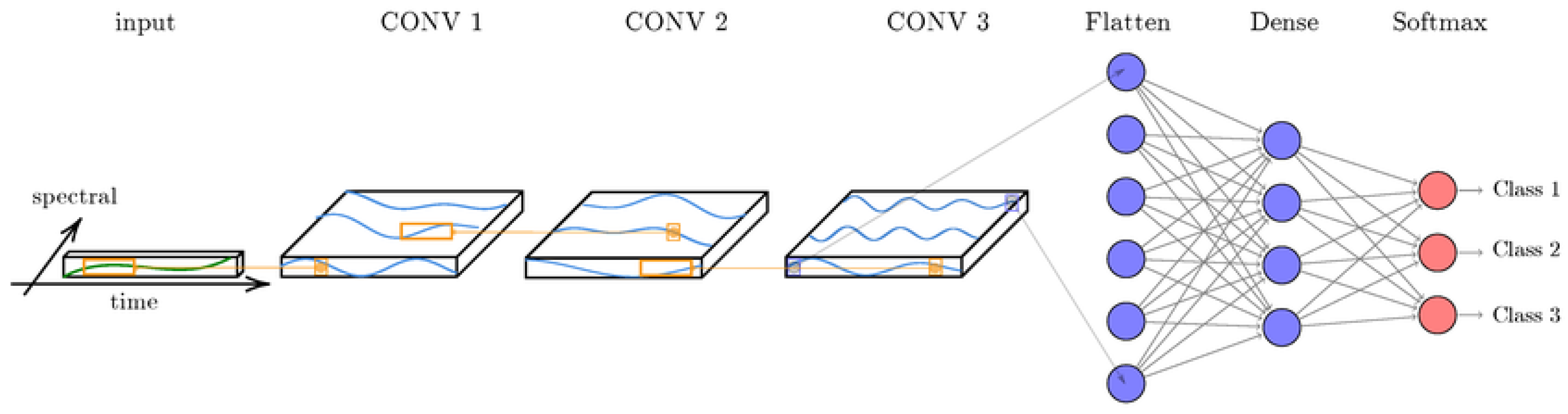
The 3DCNN consistently outperformed the 2DCNN across most configurations, underscoring the benefit of incorporating temporal information for feature extraction. The best performance was achieved with the NIR–GB combination, yielding an Accuracy of 0.93, Precision of 0.90, and Recall of 0.96, indicating the model’s strong ability to identify mining areas while maintaining few false negatives.

In contrast, the 2DCNN obtained its highest Accuracy (0.86) and Recall (0.94) with RGB–NIR bands, but showed lower Precision, suggesting that it tended to over-predict mining areas. These findings demonstrate that integrating temporal patterns via 3D convolutions enhances the model’s discriminative capacity and robustness for mining site recognition via scene classification.

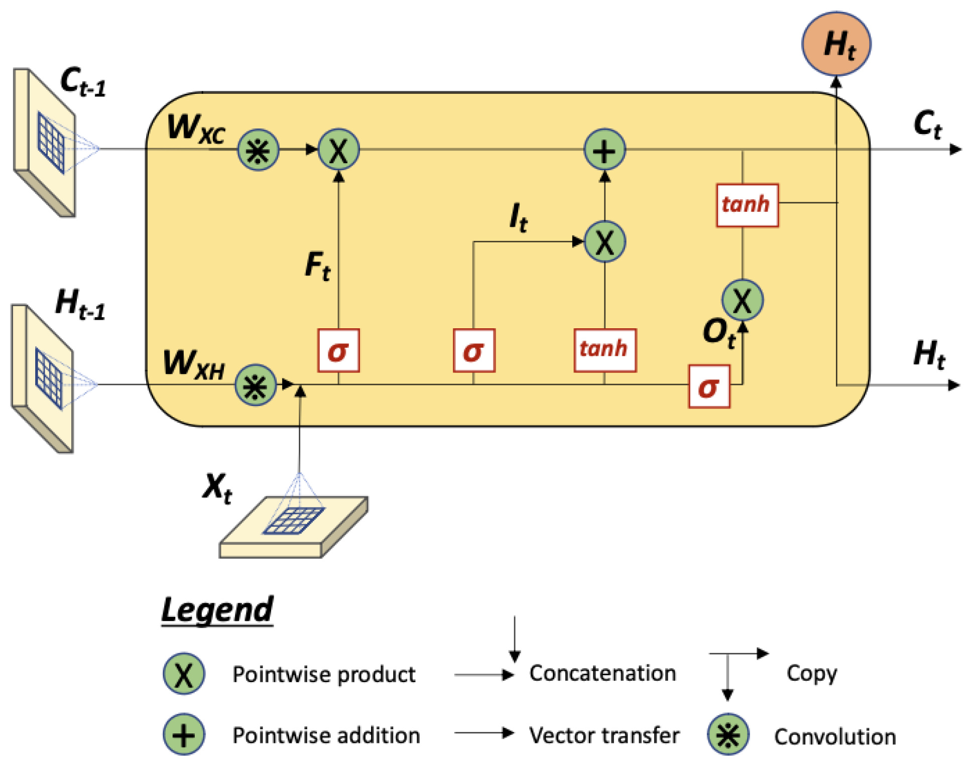
Regarding inference time, the 2DCNN presented a average latency of 0.0371 s, while the 3DCNN average latency was 0.248 s. As expected, the higher number of parameters of the 3DCNN translates into higher computational demand. However, the best performance in terms of benefit of the 3DCNN, particularly in the NIR-GB configuration where it achieved the highest F1-score (0.93) of all, mitigates this issue.

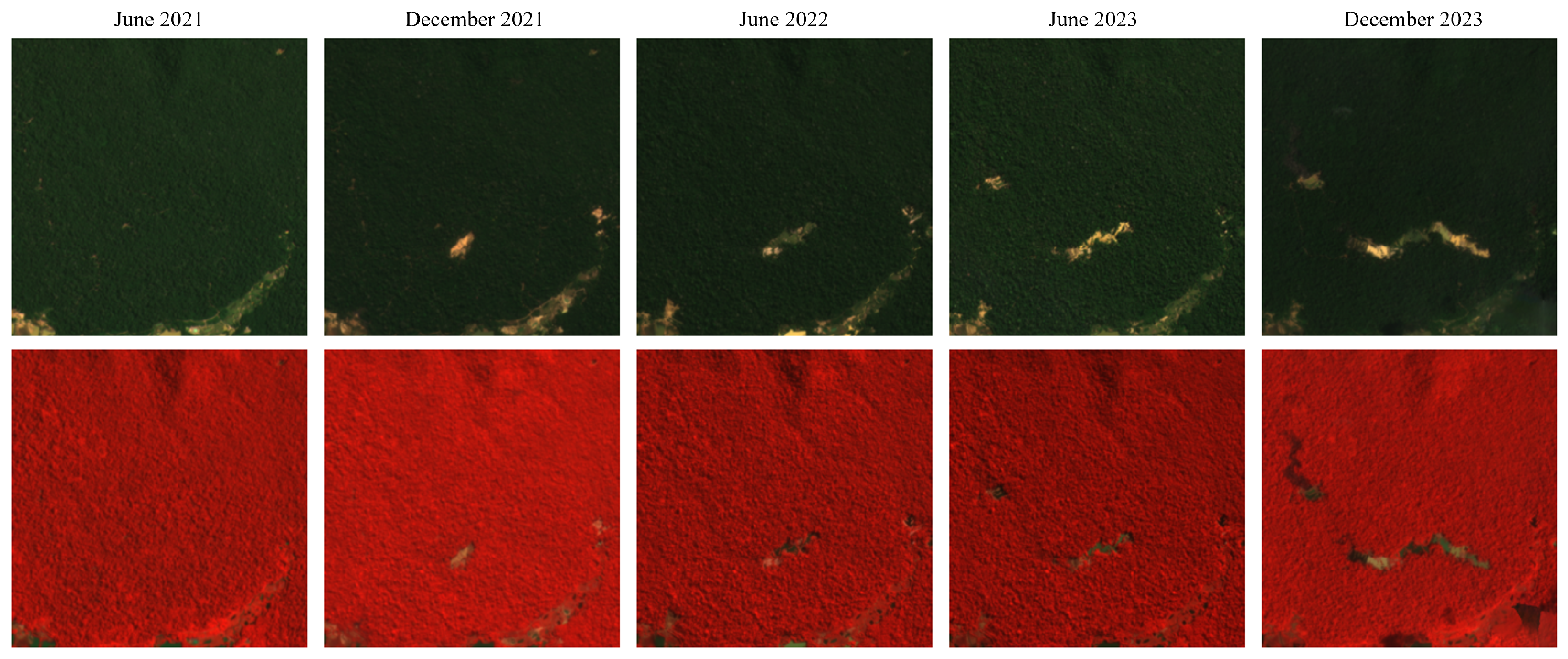
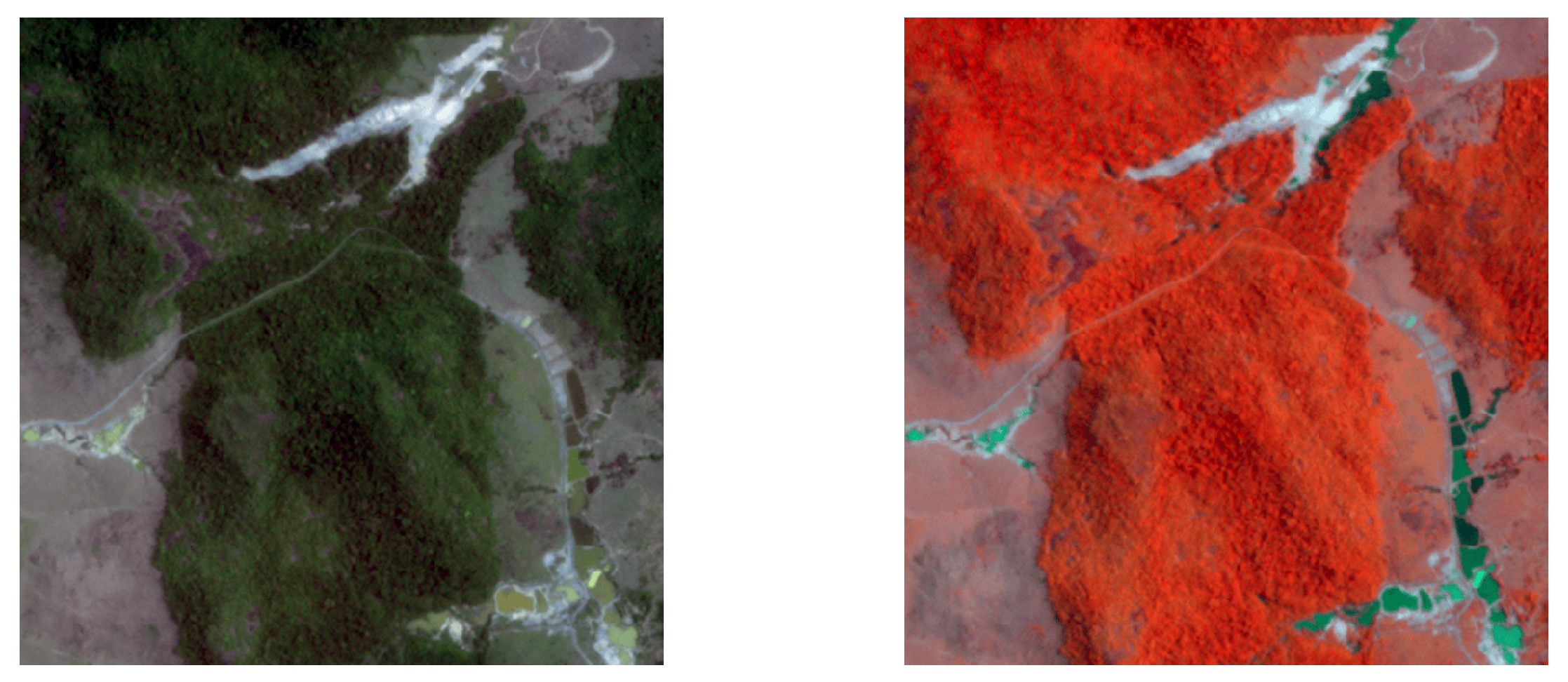
Next, we exemplify the inference from both models using the band combination that returned the highest F1-score for each, e.g., RGB-NIR for the 2DCNN and NIR-GB for the 3DCNN. Figure 13 illustrates a sample where both models correctly predicted the scene as belonging to the “Mining” class.

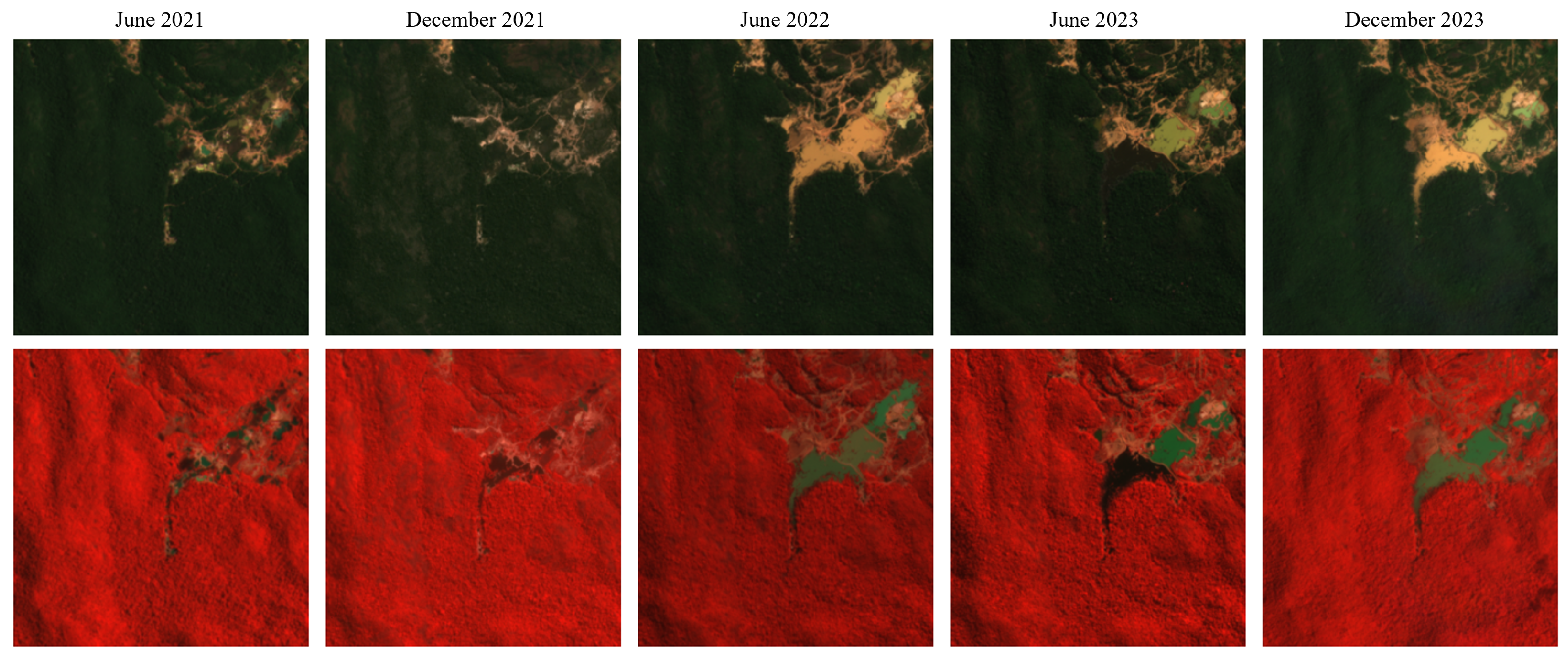
Meanwhile, Figure 14 illustrates a sample where the 3DCNN model correctly predicted as ‘Mining’ and the 2DCNN misclassified.

The sample presented in Figure 13 offers a straightforward case where the mining site exhibits distinctive spatial features like interchanging pools, allowing for both the 2DCNN and 3DCNN to correctly classify the scene as ‘Mining’. Although the sample illustrated in Figure 14 also exhibits distinctive spatial and spectral patterns, its class becomes significantly clearer when considering its evolution through time. The temporal sequence illustrates the site expansion and the progressive alteration of land cover across the five time instances.

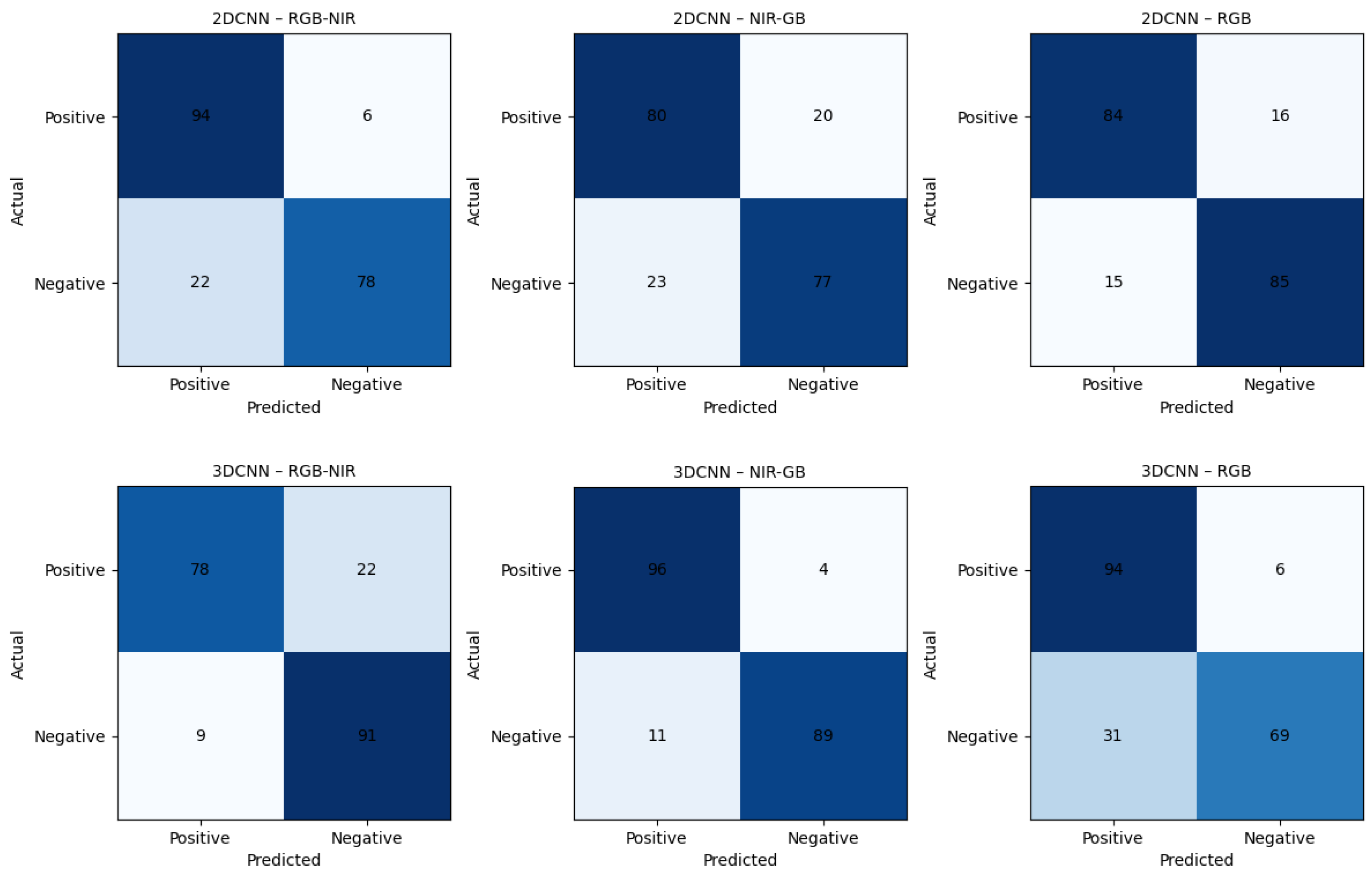
Figure 15 shows the confusion matrix for each model. Positive samples correspond to scenes containing mining sites, whereas negative samples correspond to scenes without mining activity.

The confusion matrices provided above confirm the findings in Table 5, specifically highlighting the superior ability of the 3DCNN with the NIR-GB combination to balance True Positives (TPs) and True Negatives (TNs) for the ‘Mining’ class (labeled as ‘Positive’).

4.2. Semantic Segmentation Task

Table 6. Performance comparison grouped by band configuration. In each band configuration, the best performance is shown in blue and the best overall performance considering all band configurations is shown in bold blue.

Bands	Model	Acc	Prec	Rec	F1	mIoU
RGB-NIR	U-Net	0.97 ± 0.00	0.81 ± 0.02	0.72 ± 0.00	0.77 ± 0.02	0.60 ± 0.01
	U-Net3D	0.96 ± 0.01	0.83 ± 0.01	0.49 ± 0.02	0.61 ± 0.03	0.44 ± 0.02
	CLSTM+U-Net	0.95 ± 0.00	0.70 ± 0.01	0.46 ± 0.02	0.56 ± 0.01	0.38 ± 0.01
	TempCNN	0.91 ± 0.01	0.31 ± 0.02	0.29 ± 0.05	0.34 ± 0.01	0.19 ± 0.01
	HybridSN	0.94 ± 0.01	0.57 ± 0.09	0.68 ± 0.07	0.57 ± 0.03	0.41 ± 0.02
RGB	U-Net	0.96 ± 0.00	0.80 ± 0.03	0.58 ± 0.02	0.68 ± 0.02	0.51 ± 0.02
	U-Net3D	0.96 ± 0.00	0.81 ± 0.00	0.48 ± 0.02	0.62 ± 0.02	0.45 ± 0.02
	CLSTM+U-Net	0.95 ± 0.00	0.74 ± 0.02	0.41 ± 0.04	0.53 ± 0.00	0.35 ± 0.03
	TempCNN	0.91 ± 0.01	0.40 ± 0.03	0.29 ± 0.02	0.37 ± 0.07	0.20 ± 0.01
	HybridSN	0.92 ± 0.01	0.52 ± 0.05	0.61 ± 0.08	0.54 ± 0.03	0.37 ± 0.07
NIRGB	U-Net	0.96 ± 0.01	0.70 ± 0.02	0.78 ± 0.01	0.73 ± 0.02	0.58 ± 0.01
	U-Net3D	0.95 ± 0.00	0.75 ± 0.01	0.54 ± 0.01	0.61 ± 0.01	0.47 ± 0.01
	CLSTM+U-Net	0.95 ± 0.00	0.78 ± 0.02	0.36 ± 0.01	0.51 ± 0.01	0.33 ± 0.01
	TempCNN	0.88 ± 0.02	0.35 ± 0.09	0.40 ± 0.02	0.30 ± 0.04	0.25 ± 0.04
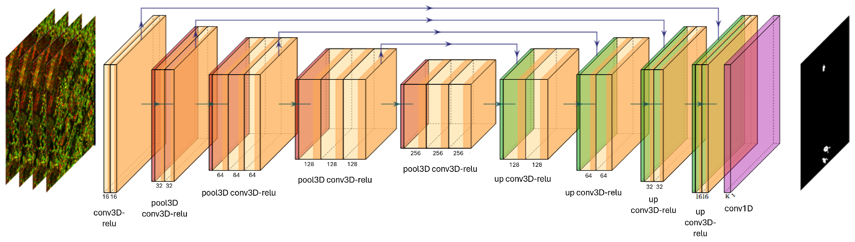
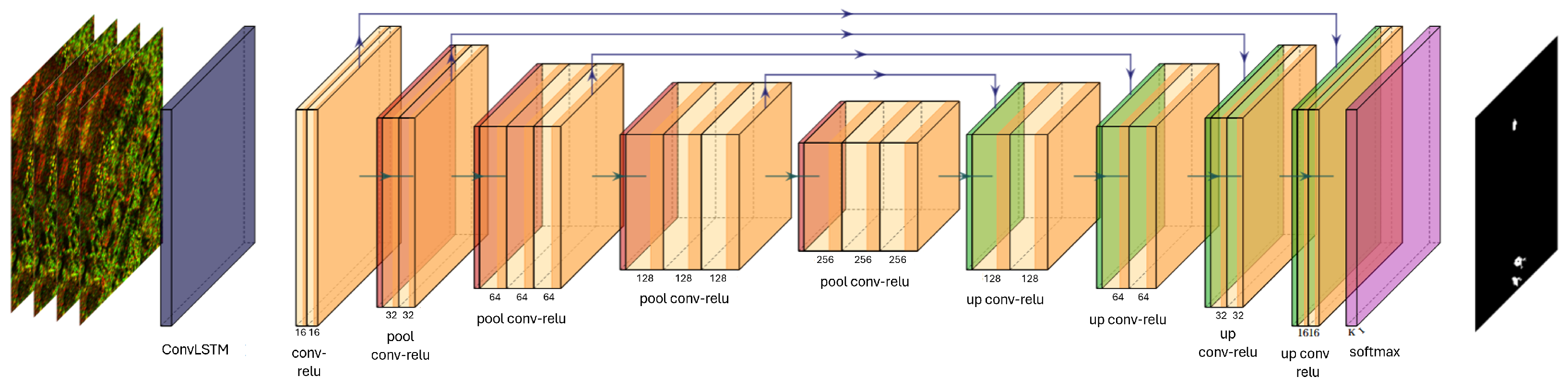
	HybridSN	0.95 ± 0.01	0.52 ± 0.06	0.63 ± 0.03	0.52 ± 0.05	0.43 ± 0.02

presents the quantitative results obtained by the U-Net, U-Net3D, ConvLSTM+U-Net, TempCNN, and HybridSN models under different spectral band configurations. We split Table 6 by band configuration for a better visualization. Each metric is the mean accompanied by its standard deviation, as explained in Section 3.4.

As shown in Table 6, the models achieved high Accuracy in all configurations, regardless of sensitivity analysis. U-Net applied to RGB-NIR bands showed the best overall performance, with an Accuracy of 0.97, F1-score of 0.77, and mIoU of 0.60. In addition, U-Net using NIR-GB bands obtained the highest Recall value (0.78).

Overall, the U-Net model showed the best performance in most band configurations. For RGB-NIR, it stood out as the best overall model, obtaining the highest Accuracy (0.97), F1-score (0.77), and mIoU (0.60) values, although U-Net3D showed greater Precision. In the RGB configuration, there was a more balanced performance, with a tie in Accuracy between U-Net and U-Net3D, but U-Net excelled in the combined metrics (F1-score and mIoU), being considered the best. In NIRGB, U-Net again showed the best overall performance, highlighting the highest Recall (0.78), F1-score (0.73), and mIoU (0.58), even with CLSTM+U-Net obtaining greater Precision. Considering all configurations, the best overall result was obtained by U-Net with RGB-NIR, highlighting the importance of the NIR band for the segmentation task. Regarding uncertainties, null values occur due to the limitation in the number of decimal places presented, in addition to the fact that the experiments were performed with only three runs due to the high computational cost of training, which may not capture small variations between the results.

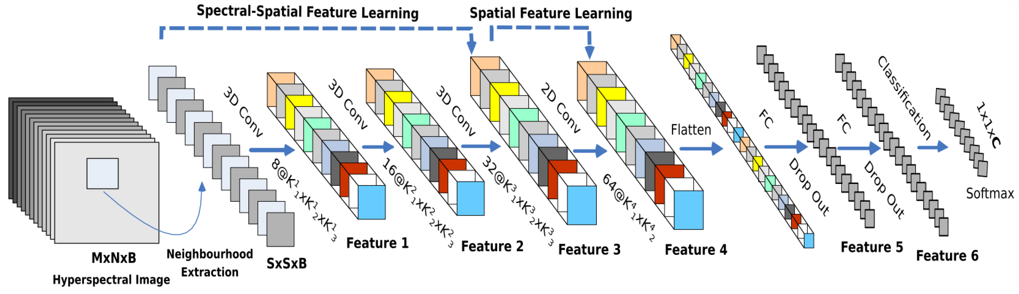
HybridSN exhibited intermediate performance, outperforming ConvLSTM+U-Net and TempCNN, but remaining below U-Net and U-Net3D. Its F1-scores ranged from 0.56 to 0.60, with mIoU values up to 0.42. These results indicate that the joint spectral–spatial modeling strategy of HybridSN provides some benefit, but is insufficient to match encoder–decoder architectures for dense segmentation tasks.

Both ConvLSTM+U-Net and TempCNN presented the weakest results. The TempCNN displayed the lowest overall performance, with an F1-score consistently around 0.33 across all band configurations. This result suggests that using the time variable alone is insufficient for effective pixel-wise mining classification. Similarly, ConvLSTM+U-Net exhibited low Recall (between 0.37 and 0.44) and F1-scores ranging from 0.50 to 0.55. This indicates that the hybrid approach struggled to effectively fuse spatial with temporal information for segmenting mining sites.

The standard deviation reveals that the U-Net(2D) and U-Net3D models demonstrate high consistency across training runs, with minimal variance in mIoU and F1-score. On the other hand, the TempCNN and HybridSN exhibit significant instability, with deviations reaching up to ±0.09 in Precision and ±0.07 in mIoU, indicating a higher sensitivity to weight initialization. That may also be because of the data shuffling, as each batch of pixels is randomly sampled from the input datacube.

Thus, the results indicate that, in this approach, the models demonstrated a greater ability to identify areas without mining activity than areas where mining is present, since the Recall and F1-score metrics, which are the most relevant for representing positive pixel hits in the predicted mask, presented lower values compared to the results of these same metrics obtained by traditional U-Net.

However, despite the U-Net achieving the highest F1-score, the U-Net3D demonstrated significantly better performance than both the TempCNN and the ConvLSTM+U-Net models. The U-Net3D achieved an F1-score of up to 0.62, which is significantly higher than the best F1-scores of 0.55 for ConvLSTM+U-Net and 0.33 for TempCNN. The U-Net3D’s high Precision (0.84) further corroborates with the scene classification results, which indicate a resilience against false positives when using the NIR band.

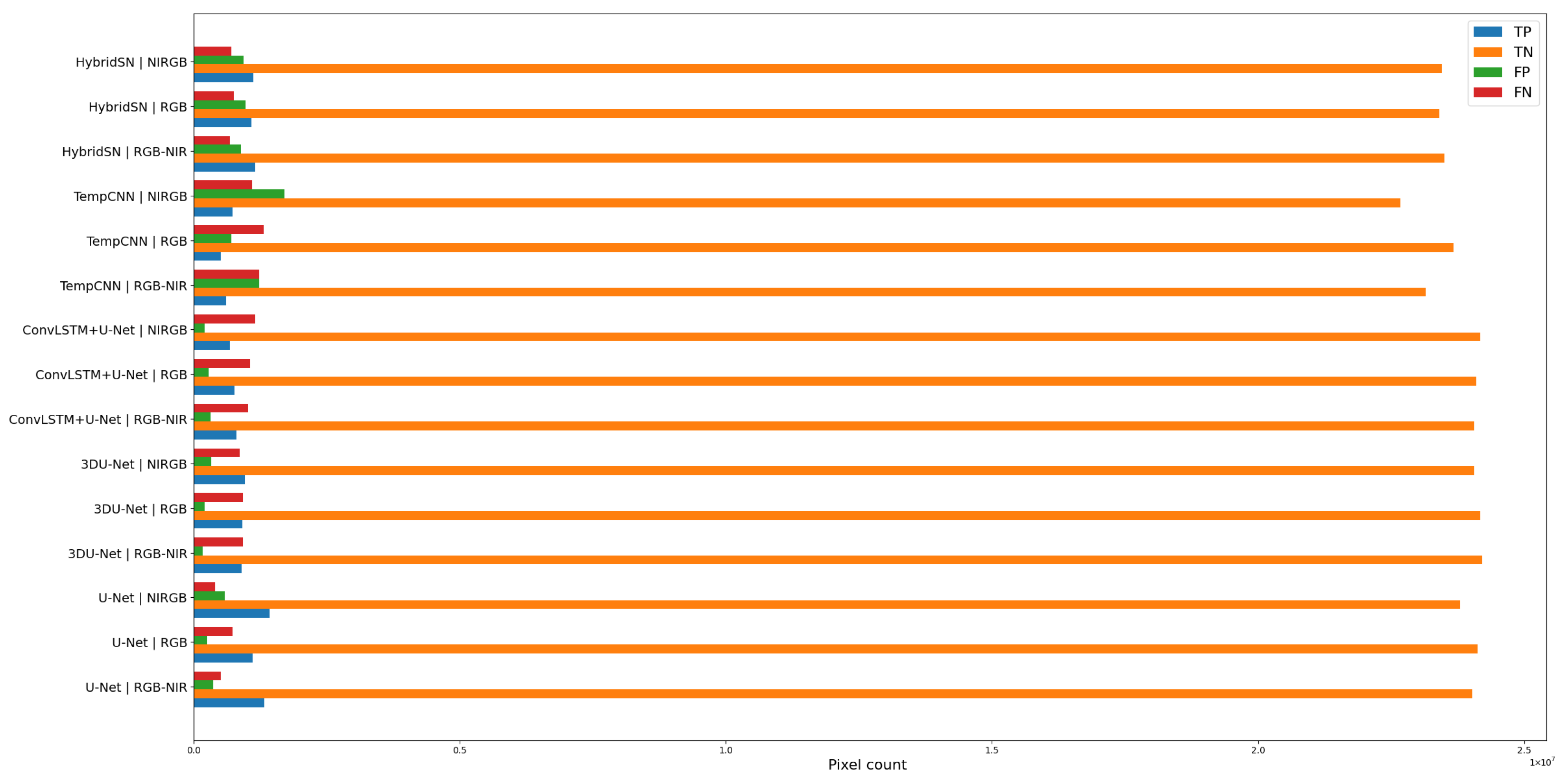
Figure 16 shows the proportion of true positives, false negatives, true negatives, and false positives from the test set due to the U-Net and U-Net3D models. As the ConvLST+U-Net and TempCNN presented poorer results, we did not include them. We can see that most pixels were classified as TN, indicating that both models have a high capacity to correctly identify areas without mining activity. In contrast, the proportion of TP is significantly lower, highlighting the difficulty the models have in detecting mined areas. This discrepancy helps us to understand why the Accuracy metric showed high values, while the other metrics, such as Precision, Recall, and F1-score, indicated less satisfactory performance.

Figure 17 provides visual examples of inference results for the two best-performing configurations (both 2D U-Nets). The predicted masks are shown alongside the corresponding reference masks for visual comparison.

Figure 17 corroborates with the metrics found. The U-Net with ResNet50 using RGB-NIR bands produces more a conservative segmentation, with fewer false positives but more omission of small mined patches, consistent with its moderate Recall. Conversely, the NIR-GB configuration yields more aggressive predictions, capturing a greater portion of mining pixels, but also introducing more commission error, in line with its higher Recall and lower Precision.

Figure 18 presents visual examples of the semantic segmentation masks generated by the U-Net3D model using the RGB-NIR and NIR-GB band combinations.

In Figure 18, we can see a similar behavior observed in the U-Net models regarding the influence of the spectral configuration. The U-Net3D using NIR-GB bands (Figure 18e) clearly shows an overestimation of the mining site area compared to when using all bands (Figure 18d). This tendency aligns with the performance metrics found for both band configuration, where the NIR-GB configuration shows a higher Recall (from 0.49 to 0.53) and lower Precision (from 0.84 to 0.75).

Table 7. Performance metrics stratified by mining polygon size for U-Net3D models. Best F1-score and mIoU per size category are highlighted in bold. These results originate from from the first training run.

Model	Bands	Size	Accuracy	Precision	Recall	F1-Score	mIoU
U-Net3D	RGB-NIR	Small	0.97	0.83	0.60	0.65	0.51
U-Net3D	RGB-NIR	Medium	0.93	0.79	0.46	0.52	0.40
U-Net3D	RGB-NIR	Large	0.86	0.89	0.50	0.58	0.46
U-Net3D	RGB	Small	0.96	0.77	0.59	0.63	0.49
U-Net3D	RGB	Medium	0.93	0.65	0.48	0.52	0.41
U-Net3D	RGB	Large	0.86	0.66	0.50	0.57	0.45
U-Net3D	NIRGB	Small	0.96	0.74	0.64	0.63	0.49
U-Net3D	NIRGB	Medium	0.93	0.72	0.52	0.56	0.44
U-Net3D	NIRGB	Large	0.86	0.76	0.56	0.59	0.49

presents the results for the performance analysis given mining polygon size. The results indicate a clear dependence of segmentation performance on mining polygon size. The U-Net3D consistently achieved the highest mIoU values for small polygons, with the best results obtained when incorporating the NIR band. Performance generally decreases for medium and large polygons, with medium-sized polygons being the most challenging.

Lastly,

Table 8. Average inference latency per sample for each model.

Model	Latency (s)
U-Net	0.039
U-Net3D	0.282
ConvLSTM+U-Net	1.862
TempCNN	0.182
HybridSN	0.014

shows the average inference latency per sample. HybridSN achieved the lowest latency (0.014 s), followed by U-Net (0.039 s). In contrast, U-Net3D, TempCNN, and especially ConvLSTM+U-Net showed substantially higher inference times. These results highlight a clear trade-off between complexity and efficiency, with U-Net offering the most favorable balance between Accuracy, segmentation quality, and latency for mining site mapping.

5. Discussion

The experiments demonstrate that the integration of temporal information via 3D convolutional operations improves the recognition of mining activities when the problem is treated as a scene classification task. Note that, for scene classification, the semantic interpretation occurs within the whole spatio-temporal volume where we assign one label per datacube. The superior performance of the 3DCNN relative to the 2DCNN indicates that temporal context enhances the model’s ability to capture subtle changes in reflectance and spatial configuration characteristic of mining sites. The temporal features likely encode vegetation loss, soil exposure, and infrastructure expansion—patterns difficult to identify from single-date imagery alone.

As shown in Figure 15, we can see that the 3DCNN models demonstrate a lower number of false positives than the 2DCNN models, especially when using the NIR band, suggesting that integrating the temporal dimension via 3D convolution helps the model to better discriminate between true mining signatures and spectrally similar land cover features.

However, this advantage did not translate into superior performance for the semantic segmentation task where a U-Net (2D) was the best approach. Note that for semantic segmentation, the goal is to have a precise spatial localization. A spatial-temporal model, like U-Net3D, usually learns spatio-temporal features jointly across all time instants. Within the U-Net3D, we have indeed considered all time instants, since a 1D convolutional serves as a temporal fusion mechanism that aggregates features from all (36) time steps: by collapsing the temporal dimension via learned weights, the model (U-Net3D) ensures that the final predicted mask is a function of the entire sequence. However, this should not be enough for semantic segmentation (pixel-based classification), requiring further investigation in the future.

The bottom line is this: while 3DCNNs are well suited for spatio-temporal modeling, their effectiveness depends strongly on the supervision strategy. As for semantic segmentation, where labels are available only for the final time step, 3D convolutions may introduce a supervision mismatch that degrades spatial localization. It is also very important to highlight that inaccurate reference annotations from the MapBiomas product may have impacted spatio-temporal models (e.g., U-Net3D) more than non-spatio-temporal models (e.g., U-Net (2D)). However, this is a point that requires further investigation. In contrast, for scene classification, where a single label describes the entire spatio-temporal patch (datacube), 3DCNNs are able to exploit temporal dynamics more effectively, leading to superior performance.

While the low-cost annotation strategy harmed all spatio-temporal approaches for semantic segmentation, U-Net3D was the best spatio-temporal approach, achieving an F1-score = 0.62 and mIoU = 0.46 (RGB configuration). Note that models like TempCNN have been used very much in practice in satellite image time-series (SITS) analysis [44]. Furthermore, U-Net3D presented the highest Precision of all models, meaning that it is highly accurate when it predicts a positive. Thus, this is an indication of the value of 3DCNNs for spatio-temporal modeling.

The spectral sensitivity analysis reinforces the importance of incorporating the near-infrared (NIR) band for mining detection. Across both tasks, combinations including NIR consistently improved Recall and mIoU. This can be attributed to NIR’s ability to discriminate vegetated and non-vegetated surfaces, making it particularly sensitive to vegetation removal and soil disturbance caused by extraction activities. However, higher Recall was often accompanied by reduced Precision, especially in NIR–GB configurations, reflecting a trade-off between omission and commission errors that was consistent across both 2D and 3D architectures.

From a computational perspective, the results reveal a clear trade-off between model complexity and inference time. While 3DCNNs improve scene classification performance, they incur substantially higher inference costs. For semantic segmentation, the U-Net offers the most favorable balance between Accuracy, mIoU, and latency, making it more suitable for large-scale and/or near-real-time mining monitoring applications. HybridSN achieves the lowest latency, but at the expense of segmentation quality.

Overall, the findings reveal a clear distinction between scene-level and pixel-level recognition of mining areas. Scene classification benefits from abstract spatial–temporal representations that capture general land-use transitions, while segmentation demands highly accurate spatial and spectral consistency.

6. Conclusions

The results obtained from this study demonstrate that, by treating mining recognition as a scene classification problem rather than a semantic segmentation one, models can get better results in terms of metrics. This is somehow expected since, in general, semantic segmentation is more challenging than scene classification, since the former demands far more detailed understanding, yields a much more complex output space, and models must balance global context and fine detail. On the other hand, scene classification usually needs only global features.

The use of 3D models, such as 3DCNN, showed the positive influence of the temporal dimension on feature extraction, contributing to a more precise identification of mined areas for scene classification. Specifically, the 3DCNN achieved the highest F1-score of 0.93 (using NIR-GB bands), demonstrating better discrimination between true mining sites and spectrally similar features compared to the 2DCNN.

For semantic segmentation, the U-Net achieved the highest scores (F1 = 0.77 and Recall = 0.72 with RGB-NIR and a ResNet50 backbone). The 3D U-Net variant followed with F1 = 0.61 and Recall = 0.549, while the hybrid ConvLSTM+U-Net and the TempCNN produced the lowest results (F1 = 0.56 and 0.34, respectively). These results indicate that, while a purely spatial approach demonstrate better performance, the U-Net3D still surpassed sequential (LSTM-based) and pure temporal (TempCNN) fusion strategies, suggesting that spatio-temporal convolution is a more effective integration mechanism, even if the added complexity limited spatial precision relative to 2D architectures.

The sensitivity analysis of the spectral bands confirmed the importance of the NIR band in both tasks, showing its importance in distinguishing between natural surfaces and areas impacted by mining activity. The NIR-GB combination proved optimal for the 3DCNN in scene classification, emphasizing the relevance of these bands for modeling temporal changes linked to mining activity.

Considering the results for both 2D and 3D CNN architectures across both tasks, the 2D CNN remain more accurate for detailed spatial delineation, leading to a superior performance in semantic segmentation with the highest F1-score. Meanwhile, the 3D CNN excelled when temporal discrimination drives class separability, resulting in the best performance for scene classification.

Future work should prioritize refining mask generation (for semantic segmentation) via spectral-index fusion and temporal composition, as well as exploring other 3D architectures. Moreover, we want to optimize model’s parameters via frameworks like Optuna [45], incorporate attention mechanisms to improve the extraction of relevant features, and adjust the temporal scale of the data to better capture the seasonal and dynamic variations associated with mining areas.