Shading and Geometric Constraint Neural Radiance Field for DSM Reconstruction from Multi-View Satellite Images

Highlights

What are the main findings?

• A general Shading and Geometric Constraint method is developed for NeRF, utilizing a spherical harmonics-based physical imaging model and a bilateral edge-aware mechanism to refine satellite image reconstruction.
• Experimental results confirm that this approach significantly outperforms existing methods, achieving up to a 57.93% reduction in elevation MAE relative to EO-NeRF, while also recovering finer structural details.

What are the implications of the main findings?

• This study provides an effective solution for handling illumination inconsistencies and shadows in satellite data, ensuring robust 3D modeling in complex scenes where traditional methods fail.
• The framework offers a practical tool for generating high-precision Digital Surface Models (DSMs), directly supporting advancements in urban digital twins, disaster monitoring, and geographic information systems.

Abstract

With the continued development of spatial information technologies, Digital Surface Models (DSMs) have become fundamental data products for urban planning, virtual reality, geographic information systems, and digital-earth applications. Neural Radiance Fields (NeRFs) have achieved remarkable success in multi-view 3D reconstruction in computer vision. Still, their application to DSM generation from satellite imagery remains challenging because of differences in imaging geometry, complex surface structure, and varying illumination conditions. To address these issues, this paper proposes a Shading and Geometric Constraint (SGC) method tailored to satellite photogrammetry and designed to integrate with existing NeRF-based frameworks such as Sat-NeRF and EO-NeRF. First, a physical imaging model based on Lambertian reflectance and spherical harmonics is introduced to represent the complex illumination variations in satellite images. Synthetic images generated by this model provide auxiliary supervision that improves robustness to illumination inconsistency. Second, inspired by classical shading-based refinement methods, we introduce a bilateral edge-preserving geometric constraint. Unlike standard smoothness terms, this constraint uses photometric discrepancies to weight geometric smoothing, thereby preserving sharp building boundaries while smoothing flat surfaces. We integrate the method into two state-of-the-art baselines, Sat-NeRF and EO-NeRF. EO-NeRF+SGC achieves up to a 57.93% reduction in elevation MAE relative to EO-NeRF, which is the largest relative MAE reduction reported in this study. The method also recovers finer structural details and sharper edges than recently published NeRF-based DSM reconstruction methods.

1. Introduction

With the rapid development of remote sensing technology, geographic information systems (GISs), and virtual reality, high-precision three-dimensional modeling of the Earth’s surface has become a critical foundation for spatial information services [1,2,3]. The DSM, as the core dataset describing the surface morphology and spatial structure, has been widely applied in urban planning, environmental simulation, disaster warning, and virtual simulation [4,5,6,7]. Compared to direct measurement using LiDAR [8], satellite imagery has become a key data source for DSM generation due to its broad coverage, rapid update cycles, and lower acquisition costs [9,10].

As a standard technique to reconstruct 3D surfaces from multi-view images, multi-view stereo has been studied for decades, yielding traditional [11,12,13] and learning-based [14,15,16,17] methods with or without the use of deep learning. However, both traditional and learning-based methods often struggle with blurred model contours and distorted geometric structures, making it difficult to meet the demands of high-precision modeling. Besides, most learning-based methods need labeled data for training, which hinders their applications.

In response to these limitations, neural implicit representation methods have recently emerged to reconstruct 3D shapes from multi-view images. Compared with traditional methods such as point clouds or voxel grids, neural implicit approaches model the color and density distributions in 3D space using neural networks, offering higher continuity and detail-preserving capability. Neural Radiance Fields (NeRFs), as one of the most representative models [18], maps spatial coordinates and viewing directions to color and density values, enabling high-fidelity reconstruction of complex geometry and illumination variations [19,20] without the need for labeled data.

Since its introduction, NeRF and its variants have driven breakthroughs in virtual reality and computer graphics. To extend its applicability, various improved models have been proposed: Deformable-NeRF [21] and NeRFies [22] handle non-rigid objects; D-NeRF [23] models dynamic scenes; and other works focus on high dynamic range [24], dark scenes [25], and computational efficiency [26,27,28,29]. These methods have significantly enhanced the practicality of NeRF in close-range and large-scale 3D modeling.

However, applying NeRF to satellite imagery presents unique challenges due to lower spatial resolution, wide-angle imaging, inconsistent acquisition times, and atmospheric scattering. To address these, researchers have tailored the NeRF framework for satellite photogrammetry. S-NeRF [30] incorporates solar illumination direction as a prior; LiDeNeRF [31] and recent depth-guided works [32] integrate LiDAR or depth priors to improve robustness. Sat-NeRF [33] and NeRF-MS [34] utilize multi-temporal images to reconstruct scene geometry and handle transient objects. More recently, CaLiSa-NeRF [35] and EO-NeRF [36] have further advanced this direction by incorporating separate streams for geometry and appearance or utilizing shadow-free albedo. Despite these progresses, current methods still face limitations in recovering geometric details in texture-less or shadowed areas and reconstructing sharp building contours, which restricts their scalability in high-precision urban modeling.

These remaining challenges highlight that 3D surface reconstruction from multi-view images is an ill-posed inverse problem. The quality of reconstructed surfaces is easy to decline when there are textureless, specular, or shadowed areas in the images. As a result, some researchers tried to model the imaging process with the Bidirectional Reflectance Distribution Function (BRDF) [37,38] into the reconstruction process, i.e., optimizing the illumination, surface albedo, and surface normal, and reconstructing 3D surfaces at the same time.

For texture-less areas, the shape from shading (SfS) technique is often used to refine the 3D surfaces. For example, Peng et al. [39] proposed a method utilizing shading information from a single-view high-resolution image to refine the low-resolution DSM, which achieves better detailed shape recovery than interpolation methods. However, the above method assumes that the direction of the incident light is known, which is hard to satisfy in a general imaging process. Thus, researchers tried to approximate the illumination with spherical harmonics to alleviate the need for the known direction of the incident light. Wu et al. [40] proposed a method utilizing spherical harmonics to refine the 3D surfaces reconstructed by MVS methods under uncalibrated illumination. Hu et al. [41] also combined the shading information and the edge information for better surface refinement in urban scenes.

To improve the physical realism and robustness of light modeling, researchers have increasingly incorporated more sophisticated BRDF models. For example, the SREVAS method [42] explicitly introduces a specular reflection component into the imaging model and employs spherical harmonics to simulate natural illumination. This approach enables accurate modeling of non-uniform albedo and non-Lambertian surfaces under complex lighting conditions, significantly enhancing the detail preservation in 3D reconstruction. However, most of the above shading-based 3D reconstruction methods did not take the imaging process into account in the reconstruction process from images, but rely on the initial surfaces recovered by MVS methods, which can cause non-optimal reconstruction results. Besides, how to better combine the shading information with the NeRF-based reconstruction process still needs further research.

Beyond pure shading cues, geometric constraints are also crucial for refining 3D surfaces. Traditional multi-view stereo methods often employ smoothness priors to reduce noise, but standard smoothness terms can blur sharp features. To address this, edge-preserving techniques, such as bilateral filtering or anisotropic diffusion, have been widely used in depth map refinement and mesh processing [43,44,45]. These methods utilize intensity gradients to guide the smoothing process, ensuring that geometric edges are preserved where photometric edges exist.

In the context of Neural Radiance Fields, integrating such physical shading models and edge-aware geometric constraints is a promising direction. By explicitly modeling the interaction between illumination and geometry and enforcing feature-preserving spatial regularity, we can potentially enhance the NeRF’s ability to recover fine structural details and reduce geometric ambiguity.

Although spherical harmonics and edge-aware priors are not new in themselves, their integration into satellite NeRF is not a direct transplantation of traditional SfS or MVS post-processing. Satellite imagery introduces wide viewing-angle changes, multi-date radiometric inconsistency, cast shadows, and complex surface materials, so illumination and geometry cannot be refined only after a stable surface has already been reconstructed. The present contribution, therefore, lies in coupling SH-based radiometric supervision and geometry-aware regularization with NeRF optimization itself, allowing density, albedo, shadow-aware shading, and normals to be adjusted jointly from multi-view satellite observations.

To address these challenges, this study proposes a general Shading and Geometric Constraint method that can be integrated into existing NeRF-based frameworks to improve DSM reconstruction.

Specifically, besides the rendering procedure of the neural radiance field, we add a physical rendering method based on the Lambertian reflectance model represented by spherical harmonics to handle the complex lighting conditions, including shadowed areas, i.e., the objective of the proposed method is to minimize the difference between the images rendered by neural radiance field and the observed images, and the difference between the images rendered by the Lambertian reflectance model and the observed images. In detail, to minimize the objective mentioned above at the same time, we estimate the surface normal from the neural radiance field.

In addition, to improve the fidelity of the reconstructed 3D surfaces, we design a geometric constraint method. Since most of the reconstructed scenes are continuous areas, we add a normal constraint to the neural radiance field, which constrains the near neighbour 3D points to have a close normal. Finally, to overcome the trade-off between noise reduction and edge preservation, we design a novel position constraint based on bilateral weights. This constraint utilizes the color similarity between neighboring rays to guide geometric smoothing. Specifically, it enforces strong position consistency in regions with similar colors while relaxing the constraint in regions with large color differences. This effectively preserves sharp building boundaries while smoothing valid surfaces.

In summary, the main contributions are as follows:

(1)

We introduced a Lambertian reflectance-based physical imaging model using spherical harmonics into the neural radiance field to tackle illumination inconsistency. The generated synthetic physical images serve as auxiliary supervision to improve the model’s robustness under complex lighting conditions.

(2)

We design a geometric feature constraint mechanism to overcome geometric distortion and blurred boundaries. The surface normals are constrained to guide model optimization and enhance the reconstruction accuracy of terrain structures and object edges. Simultaneously, we introduce a bilateral edge-aware constraint mechanism into the neural radiance field optimization. By dynamically weighting the geometric smoothness based on photometric clues, we achieve feature-preserving surface refinement, yielding sharper building edges and smoother terrains.

(3)

Qualitative experiments show that the proposed method can recover the fine detailed shapes of the ground surfaces while keeping the planar structures smooth. Quantitative experiments show that the proposed method achieves higher accuracy in terms of mean absolute error (MAE) compared with recently published NeRF-based DSM reconstruction methods. For example, when integrated into EO-NeRF, the proposed SGC reduces the elevation MAE on JAX_264 RGB from 3.064 m to 1.289 m, corresponding to a 57.93% reduction.

2. Materials and Methods

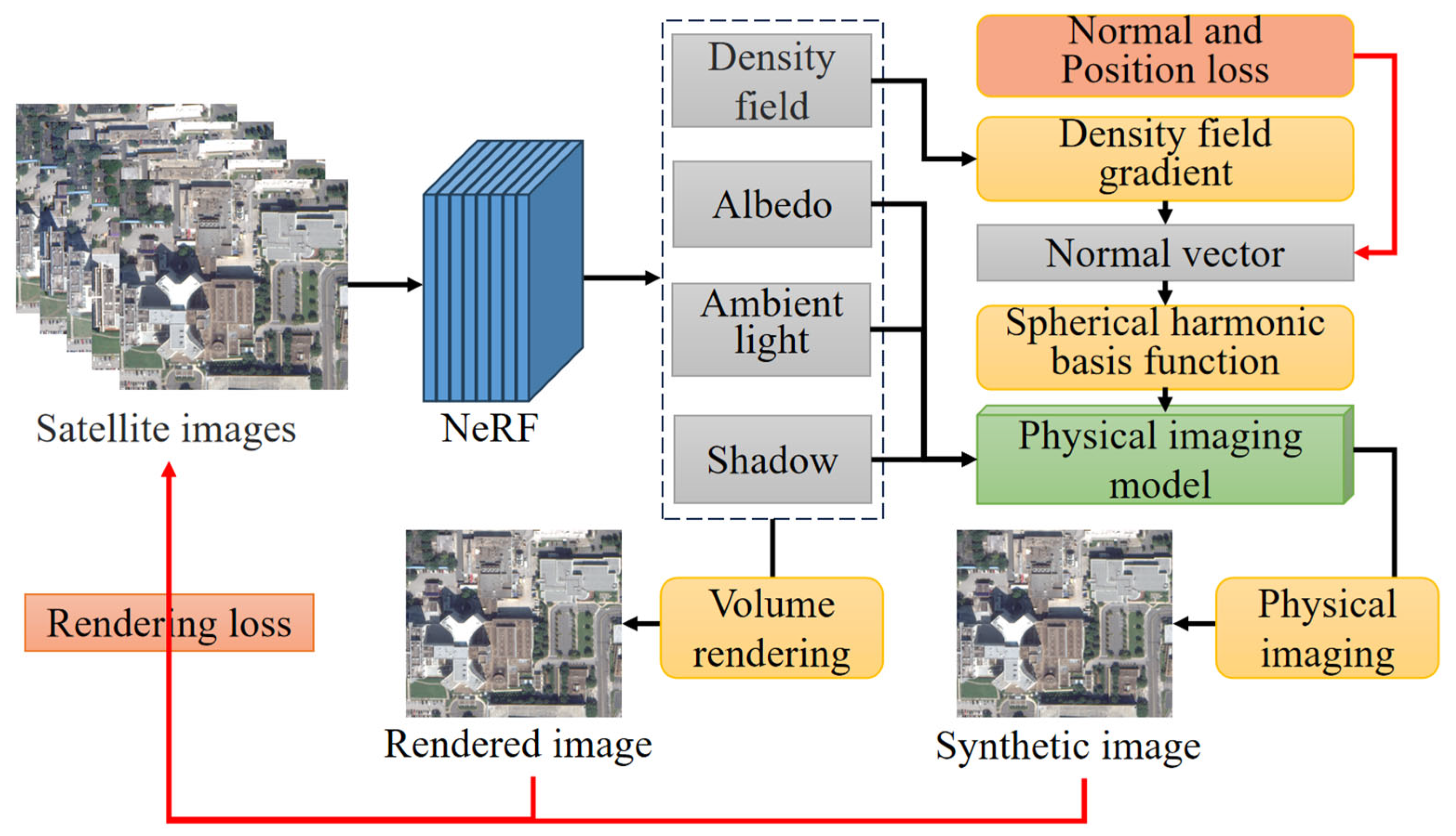
To enhance the geometric accuracy and illumination consistency of NeRF in remote sensing image-based 3D reconstruction, this paper proposes a general Shading and Geometric Constraint method that can be integrated into various satellite NeRF architectures (e.g., Sat-NeRF, EO-NeRF). The method leverages the interaction between surface geometry and incident lighting, combining a Lambertian reflectance model represented by spherical harmonic basis functions with edge-aware geometric constraints to form a unified constraint mechanism. The overall pipeline consists of two parts: the Base NeRF Backbone that predicts the scene attributes, and the proposed SGC method that imposes physical and geometric regularizations. During training, the SGC method generates synthetic images under modeled illumination and enforces structural consistency using bilateral weights derived from photometric cues. These combined losses guide the optimization of the backbone network, enabling improved reconstruction of both geometry and radiometry in complex remote sensing scenes. The overall pipeline is illustrated in Figure 1.

2.1. Shadow-Aware Irradiance Model

This study proposes a method for DSM generation by integrating NeRF with a physical imaging model. By fully leveraging the rich illumination information from multi-view satellite imagery and accurately modeling scene illumination characteristics, the proposed method enhances NeRF’s learning capability of scene density information, particularly achieving more stable predictions in shadowed regions, thus enabling the construction of more accurate three-dimensional ground models.

Vanilla NeRF samples and accumulates lighting rays to render colors by combining transmittance, opacity, and point color along the ray, as expressed in Equation (1):

$$C\left(r\right)={\sum }_{i=1}^N{T}_i{o}_i{sv}_i,$$

(1)

where ${sv}_i$ represents the shadow value at the i-th sampled point, the opacity $o_i$, and the transmittance $T_i$ are computed by Equations (2) and (3):

$$o_i=1-\exp \left(-{\mathrm{\sigma }}_i{\mathrm{\delta }}_i\right),$$

(2)

$$T_i={\prod }_{j=1}^{i-1}\left(1-o_j\right),$$

(3)

where represents the density value at the sampled point, indicating the probability that the point lies on a surface (higher implies higher opacity), and denotes the distance between adjacent sampled points along the ray.

Differently, following Sat-NeRF and EO-NeRF, we adopt the shadow-aware irradiance model to compute the NeRF-based rendering color in Equation (4):

$$I_{p1}=\mathrm{\rho }\left(P\right)\times \left(s\left(P,w\right)+\left(1-s\left(P,w\right)\right)\times a\left(w\right)\right),$$

(4)

where $\rho \left(P\right)$ is the albedo of the surface points, the shading scalar $s\left(P,w\right)$ takes values from 0 to 1, $a\left(w\right)$ is the ambient color indicating the shadowed areas.

2.2. Physical Imaging Model

To further improve model stability and accuracy under complex lighting environments, a physical imaging model is introduced. This model relies on scene attributes predicted by the NeRF and the estimated surface normals, and models illumination features using spherical harmonics. Spherical harmonics, due to their strong global representation and ability to capture low-frequency information, are widely applied in large-scale, complex illumination and spatially non-uniform 3D reconstruction tasks. Low-order spherical harmonic components are employed to model global illumination characteristics, while high-order components capture finer local illumination variations. Decomposing and reconstructing the scene illumination through spherical harmonics enables NeRF to learn radiative properties more accurately during training, thereby enhancing the geometric precision and illumination consistency of the 3D reconstruction.

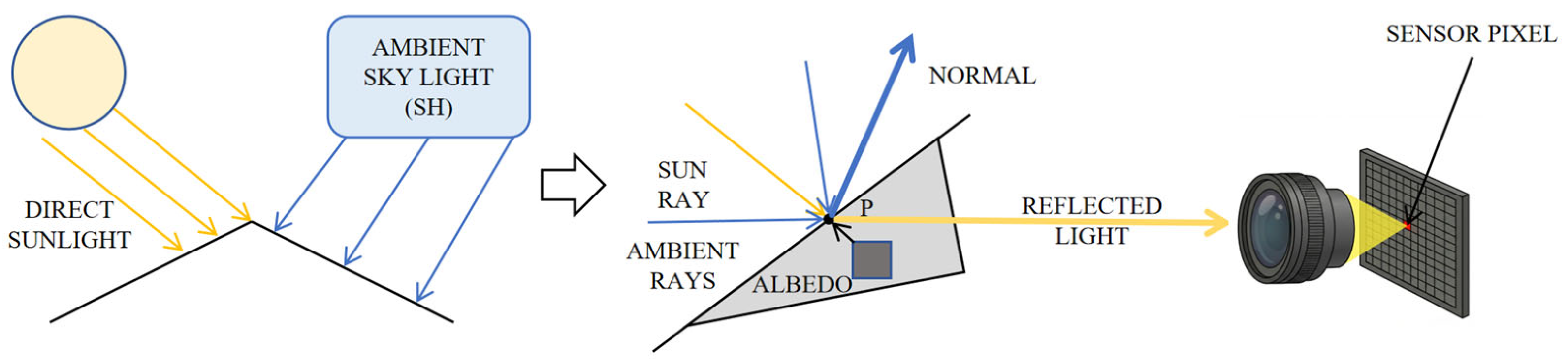
Applying the physical imaging process only as a post-processing step makes it difficult to achieve an optimal reconstruction result, because illumination and geometry would be refined only after the radiance field has already been estimated. Therefore, in this work, the physical imaging process is unified with the NeRF reconstruction procedure so that radiometric decomposition can participate directly in optimization, enabling more accurate and faithful 3D reconstruction under complex satellite imaging conditions. Specifically, we decompose illumination, albedo, and surface normals within the NeRF framework. Sunlight and ambient illumination are modeled separately rather than merged into a single term: the sunlight component is treated as a directional source associated with the solar illumination condition, whereas the spherical-harmonic coefficients are used to represent the ambient skylight field. Their combination forms the incident irradiance used by the physical imaging branch.

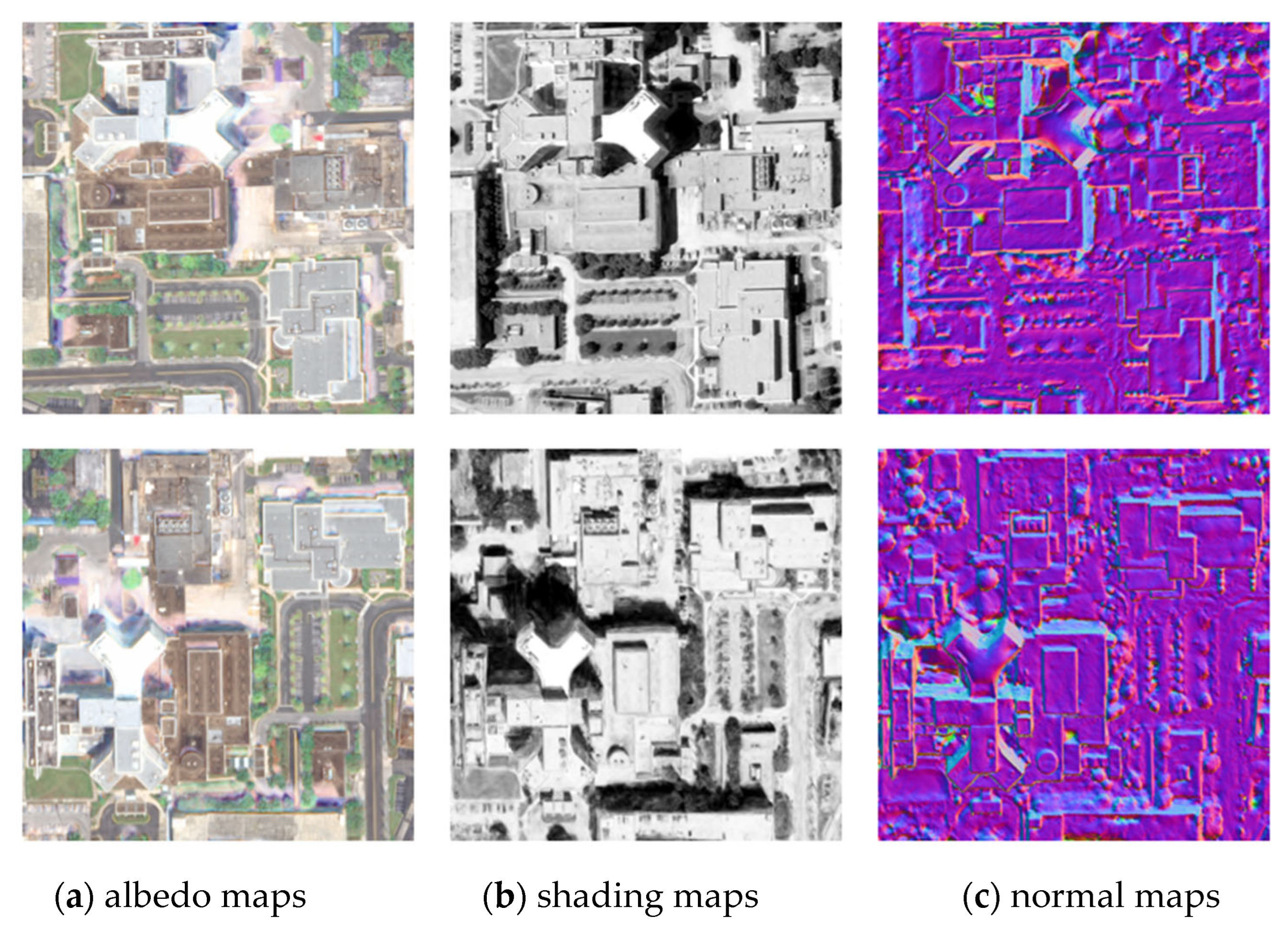
As illustrated in Figure 2, the physical imaging module is integrated into the NeRF optimization process rather than being applied only after reconstruction. Direct sunlight is modeled as a directional illumination term associated with the solar geometry, while the spherical-harmonic component represents the low-frequency ambient skylight field. These illumination terms interact with the albedo predicted by the NeRF branch and the normals extracted from the same density field to synthesize a physically constrained image. The shared shadow-aware state further modulates the balance between sunlight and ambient light, so that shadow-induced radiometric variation is explained by illumination rather than being absorbed into false reflectance changes. In this way, the module reduces lighting ambiguity and improves reconstruction fidelity in shadowed or radiometrically inconsistent regions.

In terms of detailed implementation, surface normals are extracted by calculating the gradient of the density field. The gradient of the density field $\sigma \left(P\right)$ at point P = (x, y, z) is defined in Equation (5):

$$\nabla \sigma (P)=\left(\begin{array}{c}{\displaystyle \frac{\partial \sigma }{\partial x}},{\displaystyle \frac{\partial \sigma }{\partial y}},{\displaystyle \frac{\partial \sigma }{\partial z}}\end{array}\right),$$

(5)

The unit normal vector is then obtained by normalization in Equation (6):

$$n(P)={\displaystyle \frac{\nabla \sigma \left(P\right)}{\parallel \nabla \sigma \left(P\right)\parallel }},$$

(6)

However, due to the randomness in the direction of the NeRF-predicted density gradients, the extracted normals may sometimes point in the opposite direction to the actual surface normals. Therefore, this study proposes a camera-view-based normal direction constraint strategy. Specifically, first, obtain the camera origin position op based on the camera parameters of the satellite image, and calculate the ray direction vector $d_{obs}$ = normalize (P − op) from the surface point to the camera origin in combination with the coordinates P of the sampling point. Then, the inner product between the unit normal $n\left(P\right)$ and the observation vector $d_{obs}$ is computed. If the inner product is negative, it indicates that the normal vector points away from the camera, and thus the normal vector is reversed; otherwise, the original normal is retained. This strategy ensures that all extracted normals face towards the camera, maintaining an angle less than 90°, providing stable and reliable geometric information support for subsequent physical imaging modeling.

In the physical imaging model, considering that sunlight and skylight can be approximated as distant illumination sources, this study models the lighting environment using second-order spherical harmonics. Specifically, the spherical harmonic basis functions are defined in Equation (7):

$$\begin{gathered} b_0={\displaystyle \frac{1}{\sqrt{4\pi }}},b_1=\sqrt{{\displaystyle \frac{3}{4\pi }}}{\mathrm{n}}_{\mathrm{z}},b_2=\sqrt{{\displaystyle \frac{3}{4\pi }}}{\mathrm{n}}_{\mathrm{x}}, \\ {b}_3={\displaystyle \frac{1}{\sqrt{4\pi }}}{\mathrm{n}}_{\mathrm{y}},b_4={\displaystyle \frac{1}{2}}\sqrt{{\displaystyle \frac{5}{4\pi }}}\left(3{\mathrm{n}}_{\mathrm{z}}^2-1\right),b_5=3\sqrt{{\displaystyle \frac{5}{12\pi }}}{\mathrm{n}}_{\mathrm{x}}{\mathrm{n}}_{\mathrm{z}}, \\ {b}_6=3\sqrt{{\displaystyle \frac{5}{12\pi }}}{\mathrm{n}}_{\mathrm{y}}{\mathrm{n}}_{\mathrm{z}},b_7={\displaystyle \frac{3}{2}}\sqrt{{\displaystyle \frac{5}{12\pi }}}\left({\mathrm{n}}_{\mathrm{x}}^2-{\mathrm{n}}_{\mathrm{y}}^2\right),b_8=3\sqrt{{\displaystyle \frac{5}{12\mathsf{\pi }}}}{\mathrm{n}}_{\mathrm{x}}{\mathrm{n}}_{\mathrm{y}}, \end{gathered}$$

(7)

where ${\mathrm{n}}_{\mathrm{x}}$, ${\mathrm{n}}_{\mathrm{y}}$, and ${\mathrm{n}}_{\mathrm{z}}$ denote the components of the unit surface normal $n\left(P\right)$ at the i-th surface point.

Using these basis functions, the physical imaging model can be formulated as Equation (8):

$$I_{p2}^i={\mathrm{\rho }}_i{\sum }_{k=0}^8{L}_k{b}_k,$$

(8)

where $I_{p2}^i$ represents the image intensity at the i-th surface point, ${\rho }_i$ denotes the surface albedo (including RGB channels) reflecting the material’s reflectance properties across different wavelengths, $L_k$ denotes the illumination coefficients corresponding to each spherical harmonic basis, and $b_k$ are the evaluated basis functions. The image intensity is modeled across three RGB channels, where each channel’s final illumination intensity is determined by the corresponding surface albedo ${\rho }_i$, spherical harmonic basis $b_k$, and illumination coefficient $L_k$.

Regarding loss function design, this study comprehensively considers the error between NeRF rendered images and ground truth images ($L_{rgb1}$), the error between synthetic images generated by the physical imaging model and ground truth images ($L_{rgb2}$), and the normal vector smoothness constraint ($L_{normalSM}$).

Following the uncertainty-aware training strategy, we model the photometric observations with a Gaussian distribution where the variance represents the aleatoric uncertainty. The loss $L_{rgb1}$ measuring the fitting error between the NeRF-rendered image and the ground truth is defined as the negative log-likelihood in Equation (9):

$$L_{rgb1}={\displaystyle \frac{1}{N}}{\sum }_{i=1}^N\left({\displaystyle \frac{{\left|I_{p1}^i-I_{gt}^i\right|}^2}{2{\mathrm{\beta }}_i^2}}+{\displaystyle \frac{1}{2}}log\left({{\mathrm{\beta }}_i}^2\right)\right),$$

(9)

where N denotes the total number of pixels, $I_{p1}^i$ denotes the pixel value of the NeRF-rendered image, and $I_{gt}^i$ denotes the corresponding ground truth pixel value.

Similarly, $L_{rgb2}$ measures the fitting error between the synthetic image generated by the physical imaging model and the ground truth, and is defined in Equation (10):

$$L_{rgb2}={\displaystyle \frac{1}{N}}{\sum }_{i=1}^N{\displaystyle \frac{{\left|I_{p2}^i-I_{gt}^i\right|}^2}{2{\mathrm{\beta }}_i^2}},$$

(10)

where $I_{p2}^i$ denotes the pixel value of the synthesized image, ${\beta }_i$ is the transient uncertainty predicted by the network for ray $i$.

The losses $L_{rgb1}$ and $L_{rgb2}$ in Equations (9) and (10) are both written in an uncertainty-aware form, so the predicted per-ray uncertainty downweights unreliable observations in both branches during optimization.

From a module perspective, the framework contains a NeRF rendering module and a physical imaging module that are optimized jointly rather than independently. The physical imaging module directly uses the albedo predicted by the NeRF branch, while its surface normals are extracted from the NeRF geometry represented by the same density field. In this way, the two modules share scene attributes and are coupled through a common latent representation during training.

In terms of functionality, the NeRF rendering module in Equation (4) explains the observed image through shadow-aware volume rendering, whereas the physical imaging module in Equation (8) synthesizes a physically constrained image under decomposed illumination using the shared albedo and geometry-derived normals. The same shadow state is maintained across the two modules: in Equation (4), it modulates the balance between direct illumination and the ambient component, while in Equation (8) it separates sunlight and ambient spherical-harmonic coefficients, preventing shadow-induced brightness variation from being absorbed into albedo.

2.3. Geometric Structure Constraint

To further enhance the quality of 3D reconstruction and the geometric accuracy of DSM using NeRF, we propose a geometry-aware structural optimization method consisting of two complementary terms: a Normal Smoothness Constraint and a novel Bilateral Edge-Aware Constraint. Building upon the fusion of NeRF and the physical imaging model, this approach introduces geometric features as external supervision signals. These features guide the network in accurately learning the density field distribution over the target area, thereby improving the accuracy of the elevation estimates derived from the density field.

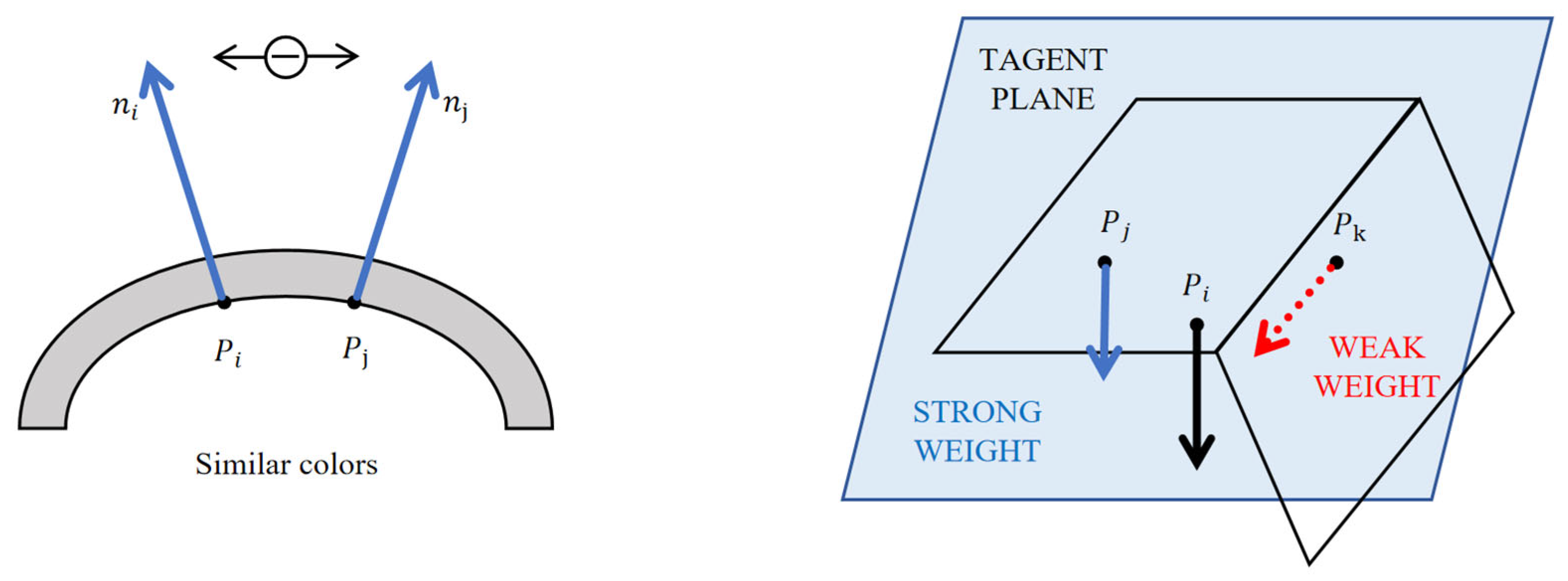
As illustrated in Figure 3, the two geometric branches play complementary roles. The normal-smoothing branch promotes local continuity in flat or homogeneous regions, but its effect is weakened when local albedo differences indicate a likely edge, thereby avoiding undesired smoothing across roofs, walls, or terrain breaks. The bilateral branch further uses the tangent plane of the center point to distinguish local noise from true structural change: neighbors that are close in both geometry and albedo receive strong regularization, whereas neighbors with inconsistent photometric cues receive weak weights and are preserved as possible discontinuities. This adaptive design is especially important for implicit NeRF geometry, because unlike explicit point-based or Gaussian-based representations, the radiance field does not provide fixed neighborhoods or surface connectivity a priori, and nearby image samples may still belong to different structures in the continuous field.

(1)

Normal Smoothness Constraint:

To ensure good continuity of the estimated surface normals in flat regions while preserving sharp features, an adaptive normal smoothness constraint $L_{normalSM}$ is introduced in Equation (11):

$$L_{normalSM}={\displaystyle \frac{1}{N}}{\sum }_{i=1}^N{M}_i\cdot {∥N_p^i-N_{near}^i∥}^2,$$

(11)

where $N_p^i$ denotes the surface normal at point $p$ and $N_{near}^i$ denotes the normal at a randomly perturbed neighboring point. In the implementation, the perturbed point is sampled by adding uniform noise in the normalized 3D space with magnitude 0.01. The edge-aware weight mask $M_i$ is computed from the albedo color difference ${\parallel c_i-c_j\parallel }_2$: $M_i=1.0$ if the difference is no larger than ${\tau }_n=0.15$, and $M_i=0.05$ otherwise.

By minimizing the discrepancy between adjacent normals, surface smoothness is maintained, thus improving the quality of subsequent 3D reconstructions. This term effectively reduces high-frequency noise on continuous surfaces.

(2)

Bilateral Edge-Aware Constraint:

Standard smoothness constraints often lead to over-smoothed results, blurring the distinct boundaries of buildings and terrain features. To address this, we introduce a Bilateral Edge-Aware Constraint $L_{bilateral}$. Inspired by edge-preserving filtering techniques, this constraint utilizes the photometric differences between neighboring rays to weight the geometric regularization dynamically.

The core idea is that significant changes in pixel color often correspond to geometric discontinuities, while similar colors imply a continuous surface. We define a bilateral weight $w_{i,j}$ for a ray $i$ and its neighbor $j$, considering both spatial proximity and photometric similarity, as shown in Equation (12):

$$w_{i,j}=\mathrm{e}\mathrm{x}\mathrm{p}(-{\displaystyle \frac{{|P_i-P_j|}^2}{2{{\sigma }_d}^2}})\cdot \mathrm{e}\mathrm{x}\mathrm{p}(-{\displaystyle \frac{{|c_i-c_j|}^2}{2{{\sigma }_w}^2}}),$$

(12)

where $P_i$ and $P_j$ denote the 3D coordinates of the center point and its j-th neighbor, and $c_i$ and $c_j$ denote their albedo features. Both constraints are guided by albedo-based photometric differences between the center point and its neighboring point(s), while the normal-smoothing branch uses a thresholded pairwise albedo difference and the bilateral branch uses continuous Gaussian weights derived from adaptive pairwise albedo differences. In the implementation, K = 4 neighbors are sampled per ray by drawing integer image-plane offsets uniformly from [−2, 2] × [−2, 2] while excluding the zero offset. The corresponding neighbor rays are rendered to recover their 3D positions. The adaptive spatial scale ${\sigma }_d$ is defined as the mean Euclidean neighborhood distance in Equation (13):

$${\sigma }_d=\sqrt{\left({\displaystyle \frac{1}{K}}\right){\sum }_j{\parallel P_i-P_j\parallel }_2^2},$$

(13)

And the photometric scale ${\sigma }_w$ is computed adaptively from local albedo differences in Equation (14), rather than being fixed as a global constant.

$${\sigma }_w=\sqrt{\left({\displaystyle \frac{1}{K}}\right){\sum }_j\parallel c_i-c_j{\parallel }_2^2},$$

(14)

Instead of directly smoothing depth values, we enforce a coplanarity constraint locally. We minimize the projected distance of neighboring points onto the tangent plane of the central point. The bilateral geometric loss is formulated in Equation (15):

$$L_{bilateral}={\displaystyle \frac{1}{N}}{\sum }_{i=1}^N{\displaystyle \frac{1}{{\overline{l}}_i}}{\sum }_{j\in {\mathcal{N}}_{\mathcal{i}}}{w}_{i,j}\cdot {\left|\left(P_i-P_j\right)\cdot n_i\right|}^2,$$

(15)

where $n_i$ is the unit normal vector at point $i$, and $\overline{l_i}$ is the average edge length used for normalization to ensure the loss is scale-invariant. This term encourages neighbors to lie on the same plane defined by the surface normal, weighted by their bilateral consistency.

The adaptive mask in Equation (11) weakens normal smoothing when local albedo differences indicate an edge, while the bilateral weights in Equation (12) jointly consider spatial proximity and photometric consistency to preserve discontinuities at roofs, walls, and shadow transitions. In this sense, the proposed masks and weights are specifically designed to make geometric regularization compatible with an implicit NeRF representation rather than assuming an already segmented explicit surface.

By minimizing this loss, the network is encouraged to smooth the geometry in texture-less or homogeneous regions while allowing for sharp depth transitions at object boundaries.

2.4. Optimization and DSM Generation

The final objective function integrates the rendering loss, physical shading loss, and the dual geometric constraints, as summarized in Equation (16):

$$L=L_{rgb1}+{\mathrm{\gamma }}_{sh}{L}_{rgb2}+{\mathrm{\gamma }}_{sm}{L}_{normalSM}+{\mathrm{\gamma }}_{bi}{L}_{bilateral},$$

(16)

where $L_{rgb1}$ is the standard NeRF rendering loss, $L_{rgb2}$ is the physical shading loss, and ${\mathrm{\gamma }}_{sh}$, ${\mathrm{\gamma }}_{sm}$, and ${\mathrm{\gamma }}_{bi}$ control the physical shading, adaptive normal smoothing, and bilateral edge-aware terms, respectively. In the implementation, ${\mathrm{\gamma }}_{sh}$ and ${\mathrm{\gamma }}_{sm}$ are selected from {0.001, 0.005, 0.01}, whereas ${\mathrm{\gamma }}_{bi}$ is selected from {0.1, 0.01, 0.001}; the final configuration for each scene is chosen according to validation performance.

Once the network is optimized, we generate the final Digital Surface Model. In this phase, this study adopts a ray integration-based depth estimation method to convert the continuous density field into discrete surface point clouds. By performing a weighted average of the sampled point depths $z_i$ along each ray, the final depth $D_f$ is computed by Equation (17):

$$D_f={\sum }_{i=1}^N{T}_i{\mathrm{\alpha }}_i{z}_i,$$

(17)

Then, combining the ray origin $o$ and the direction $d$, the 3D coordinates are obtained by Equation (18):

$$P=o+Dd,$$

(18)

Subsequently, the point cloud coordinates are transformed into geographic latitude and longitude using the RPC model, and further projected into a 2D planar coordinate system through Universal Transverse Mercator (UTM) projection, enabling the point cloud to be mapped directly into a gridded raster structure. Finally, based on the predefined spatial resolution and grid range, the elevation values of all points are mapped to their corresponding grid cells, thus completing the DSM generation process.

In summary, this section presents a comprehensive DSM optimization framework driven by the proposed Shading and Geometric Constraint method. Beyond standard surface normal computation and spatial binding, the approach introduces a novel bilateral edge-aware mechanism and physical shading supervision into the NeRF training process. This effectively addresses the limitations of traditional NeRF frameworks in elevation and structural recovery, ensuring both smoothness in flat areas and sharpness at building edges.

3. Results

3.1. Experimental Setup

To evaluate the effectiveness of the proposed method, we used the public US3D/DFC2019 Track 3 data released through the IEEE GRSS 2019 Data Fusion Contest and publicly hosted on IEEE DataPort (open access; non-IEEE members can also browse and download the released files at https://ieee-dataport.org/open-access/data-fusion-contest-2019-dfc2019 (accessed on 2 April 2026)). The source imagery consists of WorldView-3 panchromatic and 8-band visible and near-infrared (VNIR) satellite images courtesy of DigitalGlobe. According to the contest description, the native ground sampling distance is approximately 35 cm for the panchromatic band and 1.3 m for the VNIR bands, and the VNIR images released for the contest are pan-sharpened.

In this work, we follow the Sat-NeRF/EO-NeRF data preparation and use the RGB image products distributed from DFC2019: Track3-RGB-crops for the JAX_RGB setting and Track3-NEW-crops for the JAX_NEW setting. The former contains preprocessed uint8 RGB crops, whereas the latter contains float32 RGB crops pansharpened from the raw DFC2019 data. The NIR bands are not introduced as additional channels, so that the comparison remains aligned with the released Sat-NeRF/EO-NeRF RGB protocols rather than being confounded by a change in input modality. The selected areas are located in Jacksonville, Florida, USA (JAX_004, JAX_068, JAX_214, JAX_260, JAX_207, and JAX_264) and Omaha, Nebraska, USA (OMA_203 and OMA_212). At the city scale, the contest imagery was collected between 2014 and 2016 over Jacksonville and between 2014 and 2015 over Omaha.

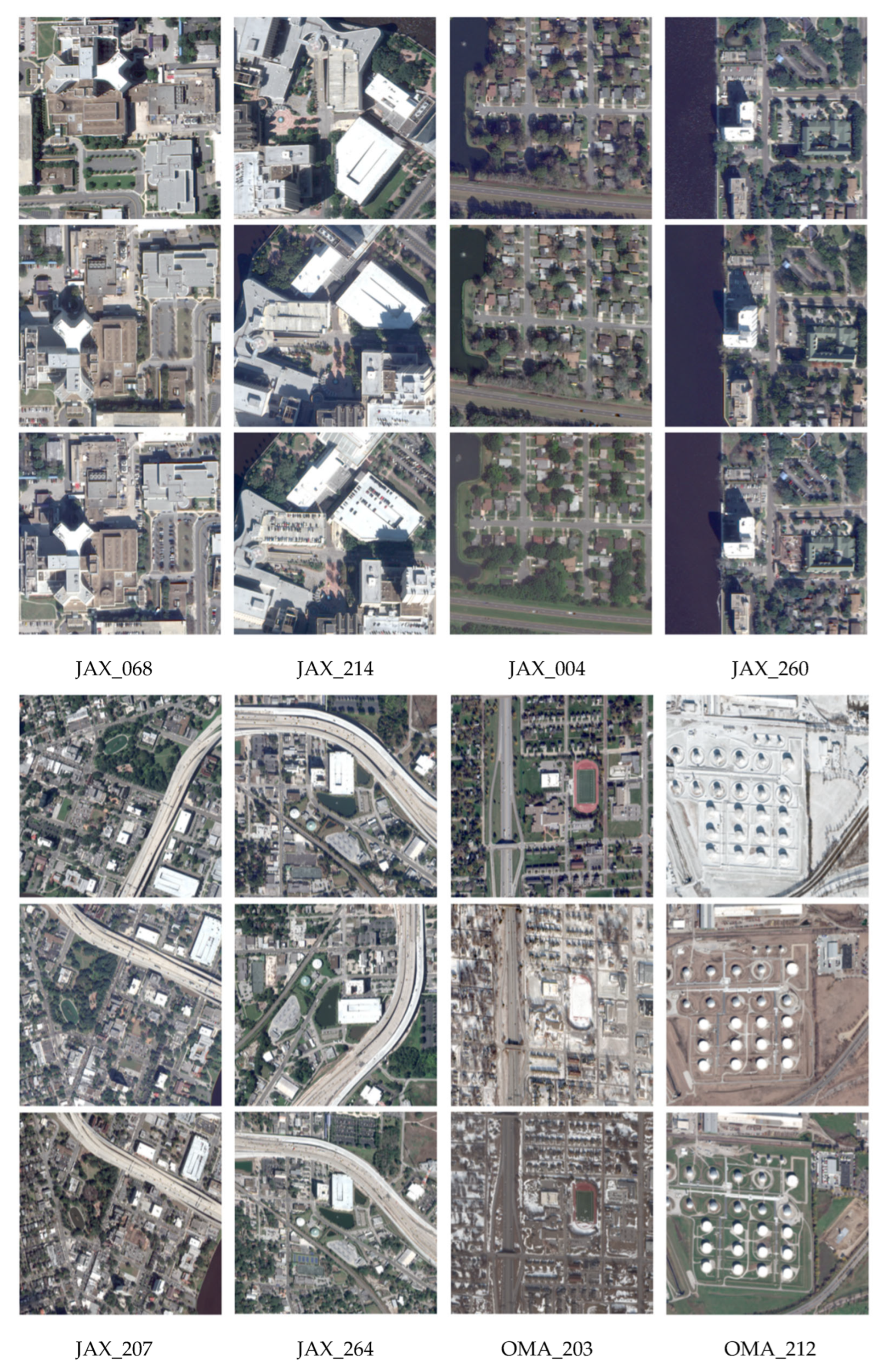
For the experimental setup used here, each target region is defined by a released Track 3 reference DSM tile of size 512 × 512 pixels at 0.5 m spacing, corresponding to an approximately 256 × 256 m ground footprint. The associated perspective RGB inputs are view-dependent image crops and therefore do not all have identical pixel dimensions after the contest preprocessing; for example, OMA_203 input views are not stored as 512 × 512 images but include sizes such as 821 × 786 and 854 × 854, even though they correspond to the same 512 × 512 reference DSM tile. As shown in Figure 4, JAX_068 and JAX_214 are dominated by dense and regular urban structures with clearly defined boundaries, whereas JAX_004 and JAX_260 contain more vegetation and irregular terrain, making 3D reconstruction more challenging. JAX_207 and JAX_264 contain larger contiguous urban layouts, while OMA_203 and OMA_212 exhibit evident radiance differences.

Table 1. Key scene information, including the number of training and test images, total sampled rays, and DSM elevation range (m).

Scene ID	Training Images	Testing Images	Total Rays Sampled	Height Range
JAX_068	17	2	613,480	[−27, 30]
JAX_214	21	3	601,292	[−29, 73]
JAX_260	15	2	612,412	[−30, 13]
JAX_004	9	2	596,276	[−24, 1]
JAX_207	21	3	569,973	[−26, 8]
JAX_264	21	3	640,306	[−29, 1]
OMA_203	37	6	590,536	[289, 328]
OMA_212	33	5	619,348	[268, 293]

summarizes the key scene information, including the number of training and test images, total sampled rays, and DSM elevation ranges in meters.

All SGC-enhanced models were trained using the Adam optimizer with an initial learning rate of 5 × 10⁻⁴. Each training batch included 1024 sampled rays, with 128 sampled 3D points per ray. The average training time required to reach convergence is discussed in Section 4.4.

To justify the choice of the edge threshold ${\tau }_n$ in the normal smoothness term, we additionally evaluated three values (0.10, 0.15, and 0.20) on four NEW scenes, namely JAX_004, JAX_068, JAX_214, and JAX_260. The average MAE values were 1.507, 1.495, and 1.521 m, respectively. The best result was obtained at ${\tau }_n$ = 0.15, indicating that an overly small threshold tends to weaken beneficial smoothing, whereas an overly large threshold may blur true geometric discontinuities. Therefore, ${\tau }_n$ = 0.15 was adopted in the reported experiments.

For evaluation, we used the airborne LiDAR-derived DSM TIFFs released in DFC2019 Track 3 as the reference geometry for all scenes. Elevation errors were computed directly between the predicted DSM and the corresponding reference DSM raster. The public Track 3 DSM files are provided as float32 TIFF products, and their GeoTIFF headers do not explicitly encode vertical-datum metadata; therefore, we follow the released benchmark convention and report elevation differences in meters with respect to the provided reference raster. Smaller errors indicate higher precision and better terrain generalization.

Accordingly, the present evaluation should be interpreted as benchmark-relative to the released DFC2019 reference raster rather than as a geodetically validated claim about orthometric or ellipsoidal height.

3.2. Method Comparison

To comprehensively evaluate the effectiveness and generalization capability of the proposed SGC method for DSM reconstruction, this section presents a series of comparative experiments. In addition to the standard NeRF-based methods (NeRF, S-NeRF, Sat-NeRF), we introduced two state-of-the-art baselines: EO-NeRF [36] and EOGS [46].

To ensure a fair and unified comparison, all methods were evaluated under the same scene-specific protocol for each available scene-format pair. Specifically, the same input images, camera metadata, reference LiDAR DSM raster, DSM grid definition, and error-computation procedure were used when comparing different methods on the same scene. MAE and RMSE were computed in the same manner for all methods. RGB and NEW results are reported separately and are compared only within the same input format rather than across formats. For the Sat-NeRF and EO-NeRF backbones, we followed the original backbone settings as closely as possible and introduced only the proposed SGC module in the enhanced variants. For scenes where the NEW-format data could not be generated because the corresponding preprocessing scripts are unavailable, the entries are marked as “/” and are excluded from comparisons requiring complete baseline coverage.

Crucially, to validate that our proposed method is a general enhancement unit, we applied it to both Sat-NeRF and EO-NeRF backbones. In

Table 2. Performance comparison of DSM reconstruction accuracy across scenes and backbones. The best results are highlighted in red, the second-best results are highlighted in blue, and the third-best results are highlighted in green. The symbol ‘↓’ indicates lower values are better. The symbol ‘/’ indicates that data were not available. Since the preprocessing scripts for the “NEW” dataset format have not been open-sourced for all regions, we were unable to generate the “NEW” dataset for scenes JAX_207, JAX_264, OMA_203, and OMA_212. In each table cell, the upper value is MAE and the lower value is RMSE.

Altitude MAE/RMSE [M] ↓
SCENE ID	JAX 068 RGB	JAX 214 RGB	JAX 260 RGB	JAX 004 RGB	JAX 207 RGB	JAX 264 RGB	OMA 203 RGB	OMA 212 RGB	JAX 068 NEW	JAX 214 NEW	JAX 260 NEW	JAX 004 NEW
NERF	2.591 3.586	2.691 4.280	3.257 4.262	3.327 4.529	2.378 3.622	2.139 3.132	5.269 6.817	1.599 3.115	/	/	/	/
S-NERF	1.496 2.490	3.687 6.008	3.245 4.312	1.830 2.634	2.233 3.436	2.307 3.658	3.855 4.807	1.759 2.500	/	/	/	/
SAT-NERF	1.276 2.389	2.126 4.124	2.429 3.638	1.417 2.273	1.909 3.228	2.107 3.749	2.966 3.978	1.605 2.365	/	/	/	/
SAT-NERF+SGC	1.243 2.399	1.922 3.806	2.181 3.522	1.329 2.221	1.890 3.191	1.442 2.176	2.518 3.302	1.209 2.274	/	/	/	/
EO-NERF	1.301 2.548	2.716 4.837	1.484 2.612	1.416 2.217	1.921 3.267	3.064 4.106	1.504 2.131	1.306 2.489	1.177 2.101	1.667 3.300	1.768 2.773	1.419 2.260
EO-NERF+SGC	1.283 2.543	2.447 4.143	1.448 2.491	1.352 2.191	1.908 3.297	1.289 2.425	1.362 1.936	1.111 1.758	1.087 2.163	1.553 3.251	1.452 2.439	1.387 2.209
EOGS	/	/	/	/	/	/	/	/	1.112 2.215	1.750 3.568	1.553 2.624	1.393 2.459

, ‘Sat-NeRF+SGC’ denotes the Sat-NeRF model integrated with our SGC method, while ‘EO-NeRF+SGC’ denotes the EO-NeRF model enhanced by the same method. MAE remains the primary elevation indicator, but for a more comprehensive assessment, Table 2 reports scene-wise MAE on the first line and RMSE on the second line, both in meters. Additional structure-aware metrics are further summarized and discussed in Section 4.1.

As shown in Table 2, the proposed method consistently improves the reconstruction accuracy across different backbones. The RMSE values follow the same overall trend as the MAE values, further confirming that the proposed SGC module improves both average elevation accuracy and robustness to larger errors.

Improvement on Sat-NeRF: When integrated with the Sat-NeRF backbone, our ‘Sat-NeRF+SGC’ model achieves a reduction in Mean Absolute Error (MAE) across all evaluated scenes compared to the baseline. This improvement is particularly notable in scenarios with complex surface structures. For instance, in JAX_260 and JAX_004, which feature irregular terrain, the method demonstrates enhanced adaptability. Furthermore, in the JAX_264 scene, the accuracy improves substantially from 2.107 m to 1.442 m, proving the method’s strong capability in correcting geometric distortions in challenging environments.

Improvement on EO-NeRF: The efficacy of our approach is even more pronounced when applied to the advanced EO-NeRF architecture. For the JAX_264 RGB scene, the EO-NeRF baseline yields an elevation MAE of 3.064 m, whereas EO-NeRF+SGC reduces this value to 1.289 m. On the NEW-format scenes, the method also improves the JAX_214 and JAX_260 areas from 1.667 m to 1.553 m and from 1.768 m to 1.452 m, respectively. These gains confirm that introducing explicit physical shading models and bilateral geometric constraints brings substantial benefits, even to state-of-the-art frameworks.

Comparison with State-of-the-art: Our enhanced model also demonstrates superior performance compared with the emerging 3D Gaussian Splatting baseline EOGS [46] on the scenes where NEW-format results are available. For example, on JAX_214 and JAX_260, EO-NeRF+SGC achieves lower elevation MAE values than EOGS (1.553 m vs. 1.750 m on JAX_214 and 1.452 m vs. 1.553 m on JAX_260). Additionally, on JAX_068, our method achieves an MAE of 1.087 m, slightly lower than the 1.112 m obtained by EOGS. This evidence establishes that NeRF-based methods, when equipped with our SGC module, remain a top-tier solution for high-precision satellite photogrammetry.

EOGS also shows that explicit and implicit representations have different strengths for this task. As an explicit Gaussian-based representation, EOGS can optimize local surface structure more directly and can therefore be highly competitive in scenes with stable radiometry and clear geometric support. By contrast, the implicit NeRF formulation remains attractive when radiometric decomposition and shadow-aware supervision are important, because density, albedo, shading, and geometry can be optimized within one continuous field. The results in Table 2, therefore, suggest a complementary picture rather than a one-sided dominance: EOGS is strong in some scenes, while EO-NeRF+SGC is particularly effective when shadow ambiguity and radiometric inconsistency become major error sources.

In summary, the quantitative results in Table 2 confirm that the proposed SGC method is not limited to a specific network but serves as a generalizable plug-in that universally enhances geometric fidelity and elevation accuracy in diverse remote sensing scenarios.

A scene-specific reading of Table 2 shows that the gains of EO-NeRF+SGC are not uniform across all regions. The largest MAE reductions appear in scenes where radiometric inconsistency, strong shadow effects, or more evident geometric ambiguity are present, such as JAX_264 RGB (3.064 m to 1.289 m), OMA_212 RGB (1.306 m to 1.111 m), OMA_203 RGB (1.504 m to 1.362 m), and JAX_260 NEW (1.768 m to 1.452 m). The NEW inputs are pansharpened from the DFC2019 raw data, so their radiometric characteristics are not identical to those of the original RGB imagery; in such cases, the added physical imaging and geometric constraints provide especially useful complementary guidance beyond the EO-NeRF baseline.

By contrast, the improvements are more modest in JAX_068 RGB (1.301 m to 1.283 m), JAX_260 RGB (1.484 m to 1.448 m), JAX_207 RGB (1.921 m to 1.908 m), and JAX_004 NEW (1.419 m to 1.387 m). These cases suggest that the EO-NeRF baseline already provides comparatively stable reconstruction when illumination inconsistency is less dominant, so the room for further global MAE reduction becomes smaller. In addition, some remaining errors in these scenes are still related to vegetation, fine irregular structures, and local boundary complexity, which are only partially addressed by the current SGC design. The three RGB scenes represent native observations with relatively limited shadow-driven ambiguity, whereas JAX_004 NEW is a pansharpened product derived from the DFC2019 raw data and is additionally affected by vegetation and non-rigid canopy structure. Overall, this scene-dependent behavior indicates that SGC is most beneficial when radiometric decomposition and edge-aware regularization directly target the dominant source of reconstruction error.

3.3. Three-Dimensional Model Visualization and Qualitative Performance Assessment

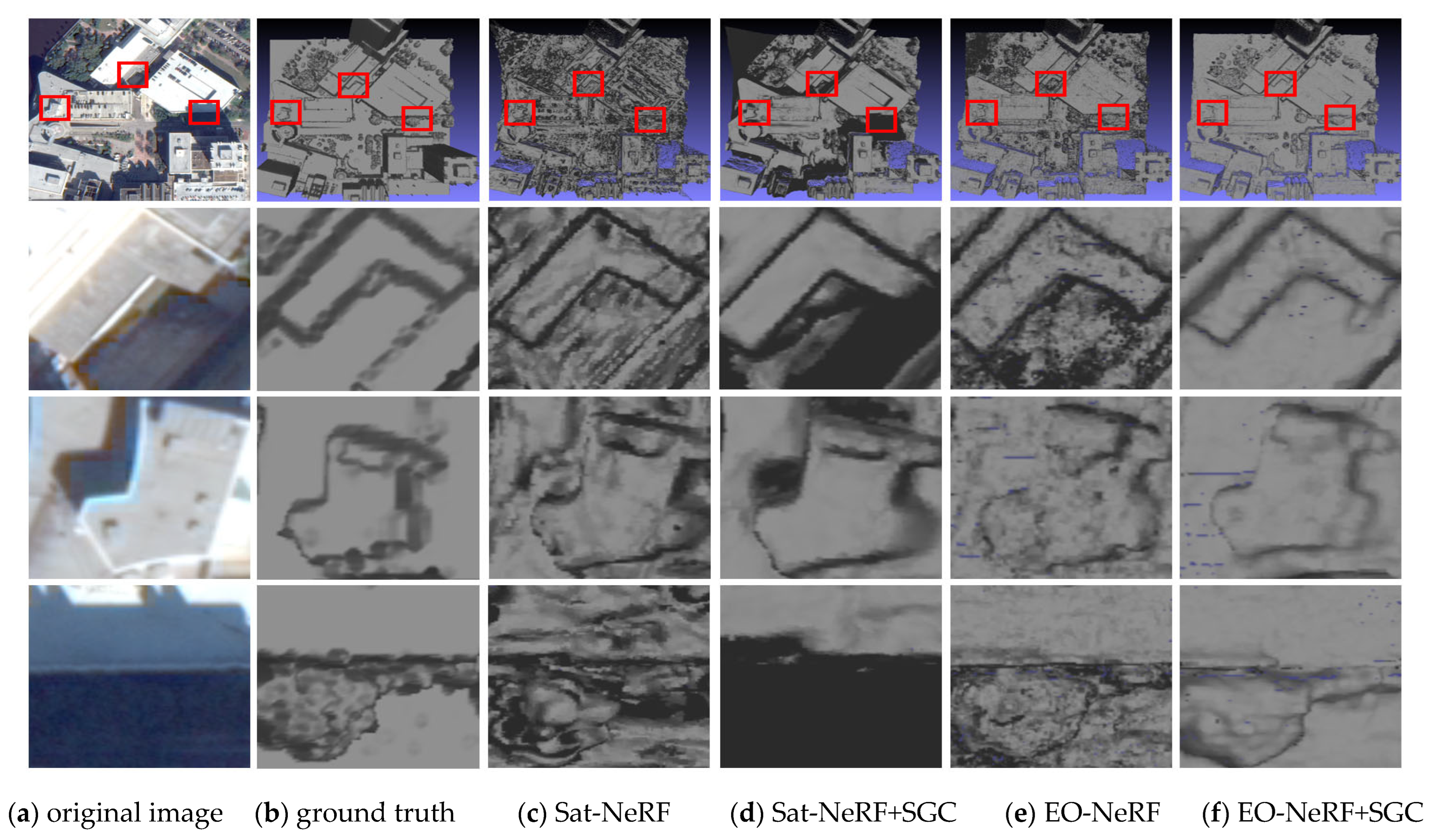
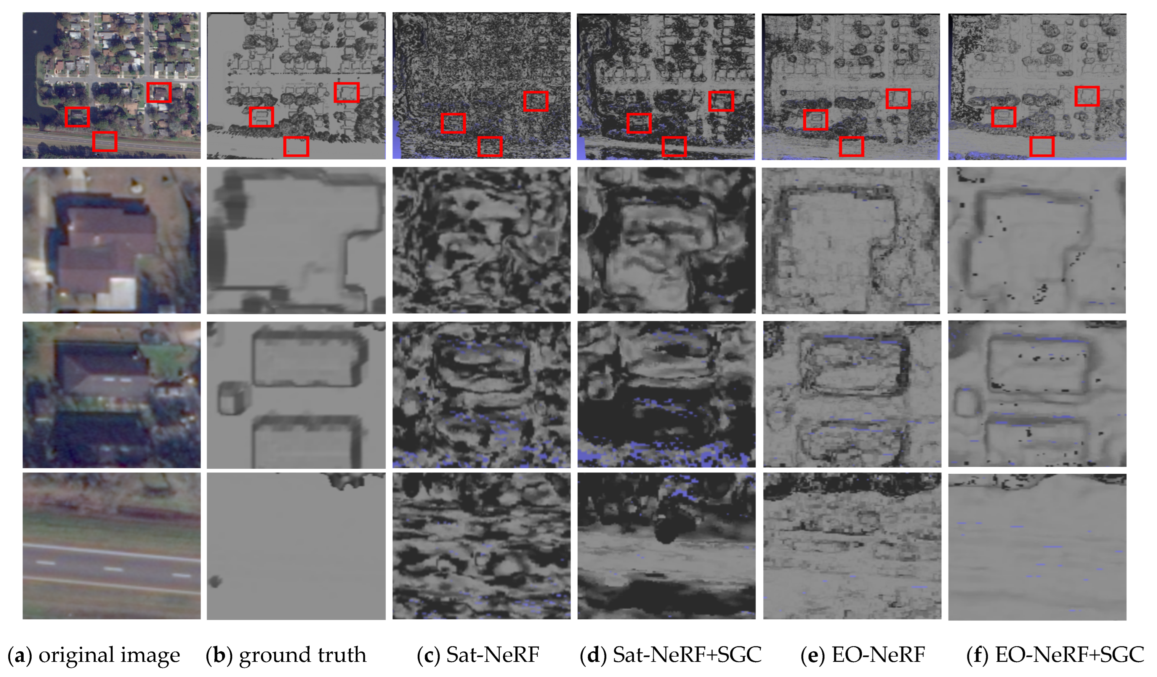
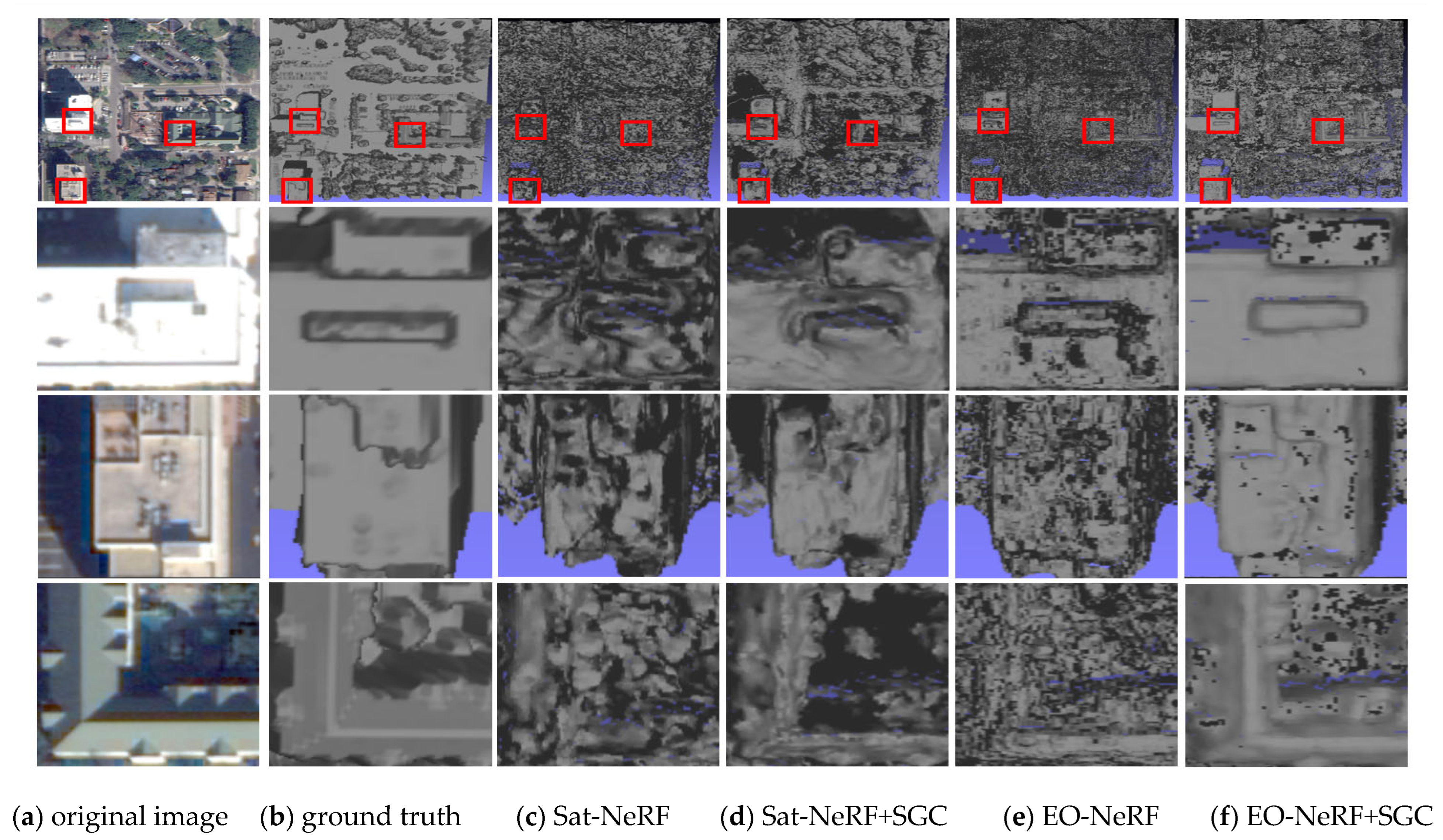
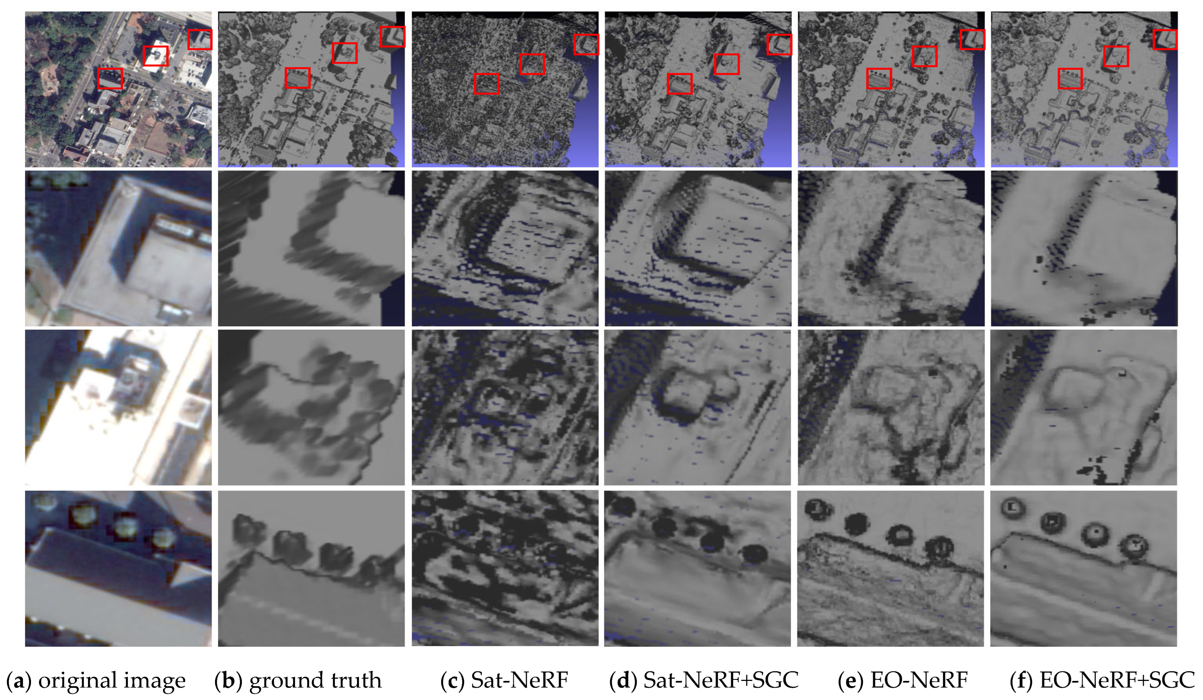
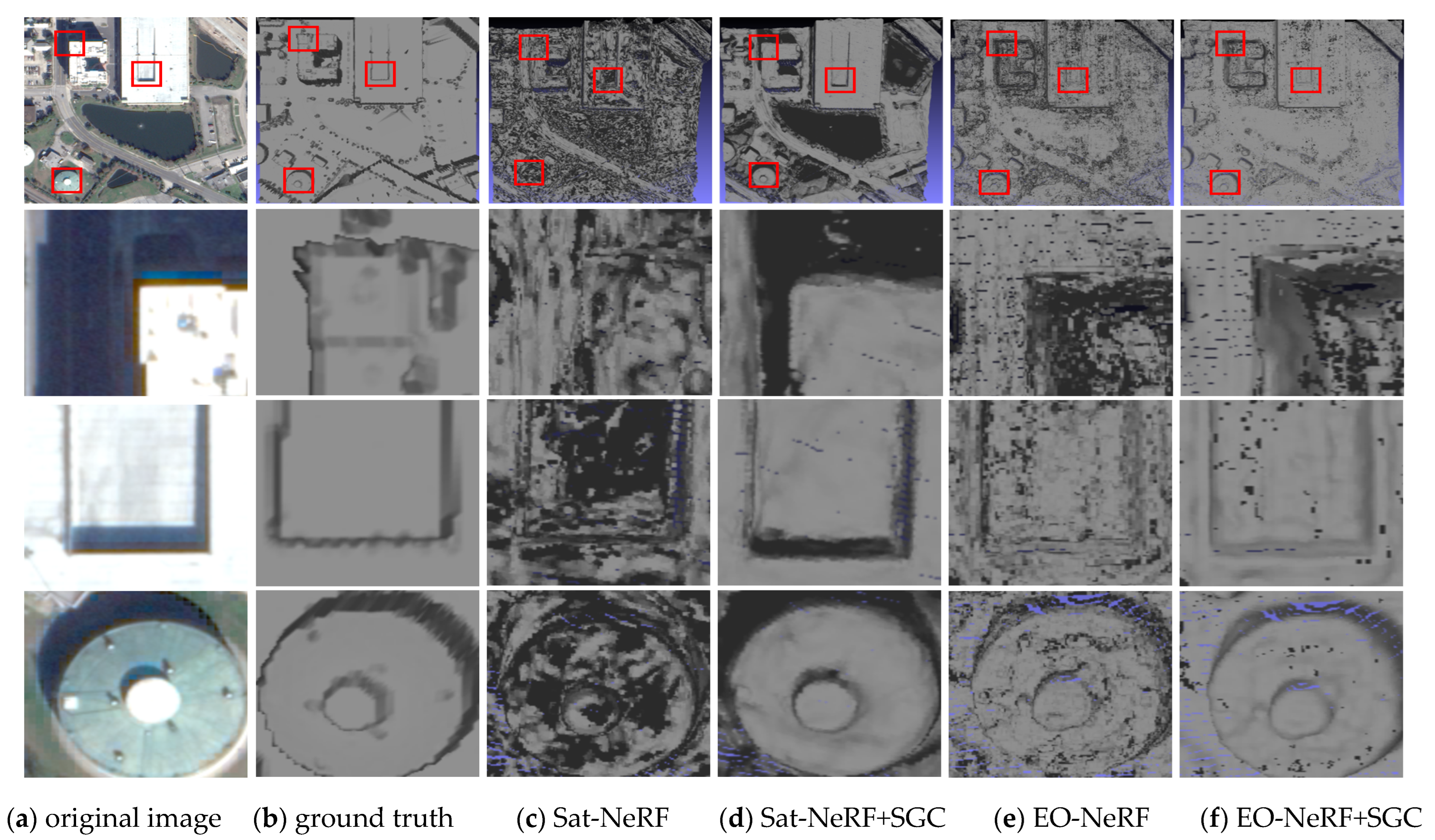
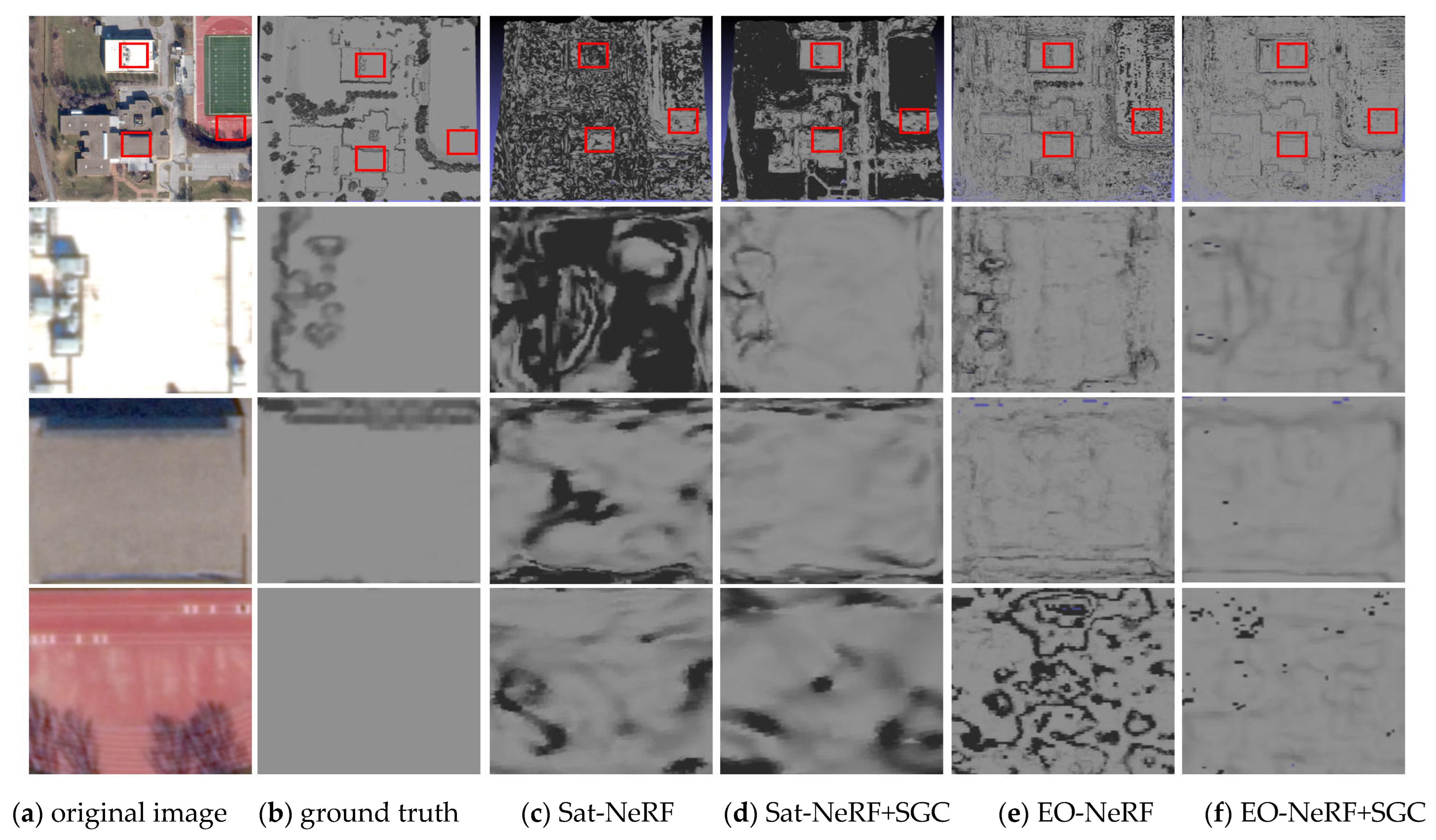
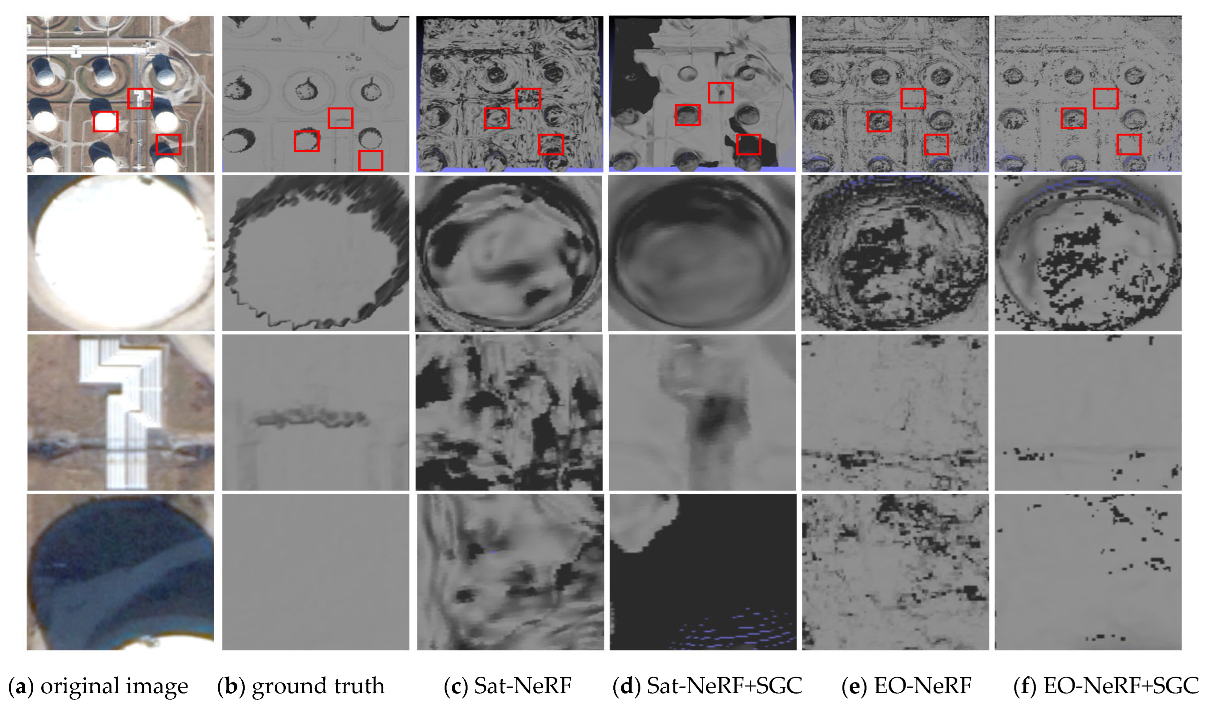
To further validate the effectiveness and robustness of the proposed method, this section presents a comparative 3D visualization analysis of DSM generated by the ground truth, baseline Sat-NeRF, Sat-NeRF+SGC, the baseline EO-NeRF, and EO-NeRF+SGC under mesh representation. Through direct visual inspection, the differences in reconstruction quality, geometric consistency, and model completeness can be clearly observed, providing deeper insight into the practical performance of each method. Figure 5, Figure 6, Figure 7, Figure 8, Figure 9, Figure 10, Figure 11 and Figure 12 present the visualized details of the 3D models reconstructed for the eight target regions in the experiments. By comparing the detailed areas highlighted with red rectangles, it can be verified that the proposed method demonstrates significant advantages across multiple aspects.

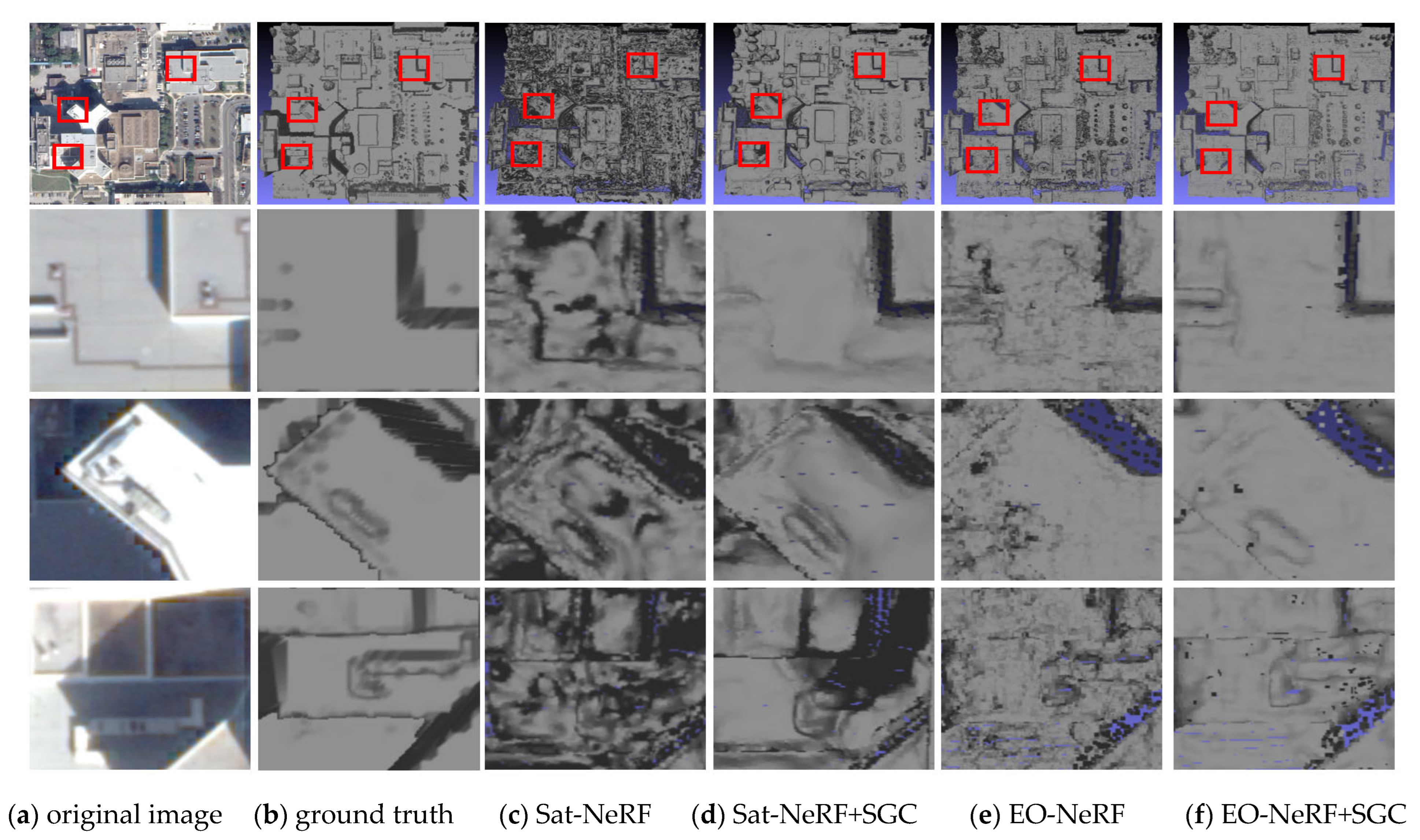
As highlighted by the red bounding boxes in Figure 5 and Figure 6, which are dominated by dense and regular urban structures with clearly defined boundaries, the SGC module improves geometric reconstruction across both backbones.

In these regions, the baseline Sat-NeRF exhibits severe planar distortion and noise, which blur edges and fragment the reconstructed structures. EO-NeRF improves the overall layout, but still shows noticeable surface roughness and jagged artifacts along building boundaries.

After SGC is introduced, both backbones improve visibly. Sat-NeRF+SGC reduces much of the distortion present in Sat-NeRF and produces smoother surfaces and clearer shapes, indicating that the module can correct substantial geometric errors. EO-NeRF+SGC yields the cleanest results overall, preserving the structural advantages of EO-NeRF while further suppressing residual noise and sharpening building transitions. As a result, EO-NeRF+SGC provides the most complete meshes and the clearest building facades among the compared methods.

As highlighted by the red bounding boxes in Figure 7 and Figure 8, which contain abundant vegetation and irregular terrain, the proposed SGC method improves the reconstruction of complex landscape details.

In these scenes, the baseline Sat-NeRF struggles to separate vegetation from terrain structure, producing noisy 3D outputs with limited local detail. EO-NeRF captures the overall layout more reliably, but still exhibits surface roughness and unstable texture-geometry separation, especially where dense vegetation covers the ground.

With SGC, reconstruction quality improves for both backbones. Sat-NeRF+SGC reduces noise and clarifies the shapes of buildings and terrain, showing that the module can recover part of the missing structure. EO-NeRF+SGC gives the best results overall, with clearer separation between vegetation and uneven terrain and fewer visible artifacts. By combining the stronger EO-NeRF backbone with the proposed radiometric and geometric constraints, it produces a more faithful reconstruction of these challenging scenes.

As highlighted by the red bounding boxes in Figure 9 and Figure 10, which contain larger contiguous urban layouts, the proposed SGC method improves geometric consistency while preserving local detail.

The baseline Sat-NeRF performs poorly in these larger contiguous urban scenes and fails to recover the overall layout reliably. EO-NeRF captures the global structure more successfully, but still lacks local refinement: building boundaries remain ragged, and the surfaces show noticeable noise and granularity.

The SGC-enhanced models improve both global completeness and local detail. Sat-NeRF+SGC restores much of the missing structural continuity relative to its baseline and yields a more coherent overall layout. EO-NeRF+SGC again provides the best reconstruction quality, preserving large-scale organization while producing sharper building boundaries and smoother transitions between urban zones.

As highlighted by the red bounding boxes in Figure 11 and Figure 12, where the input images exhibit pronounced radiance differences, the proposed SGC method improves geometric reconstruction under challenging illumination variation.

Under these conditions, the baseline Sat-NeRF is strongly affected by radiometric inconsistency, producing fragmented meshes with blurred edges and unstable geometry. EO-NeRF improves boundary definition, but still suffers from high-frequency surface noise and visible artifacts.

After SGC is added, both models better disentangle geometry from brightness variation. Sat-NeRF+SGC produces more coherent surfaces and preserves geometric boundaries more reliably than the baseline. EO-NeRF+SGC yields the best overall result, further reducing residual noise and recovering more faithful structural detail in these radiometrically inconsistent scenes.

Across the four scene categories—dense regular urban areas (JAX_068, JAX_214), vegetation-rich and irregular regions (JAX_004, JAX_260), larger contiguous urban layouts (JAX_207, JAX_264), and scenes with pronounced radiance variation (OMA_203, OMA_212)—the proposed SGC method consistently improves the baseline reconstructions.

When applied to either Sat-NeRF or EO-NeRF, the SGC module improves reconstruction quality. In regular urban scenes, it sharpens building boundaries and completes facades; in vegetation-rich and irregular scenes, it recovers finer terrain and object separation; in larger urban layouts, it better balances global structural consistency with local detail; and in radiometrically inconsistent scenes, it better separates geometry from brightness variation.

Overall, EO-NeRF+SGC provides the most robust performance by combining the strengths of EO-NeRF with the radiometric and geometric regularization introduced by SGC. These results support the effectiveness of the proposed method across diverse and challenging reconstruction scenarios.

3.4. Ablation Study

Table 3. Elevation MAE (m) of EO-NeRF ablations with BI, BI+SM, and the full GC+PIM configuration. Table 3 shows that the full EO-NeRF+SGC setting achieves the lowest MAE in all listed scenes, while the intermediate BI and BI+SM rows reveal how edge preservation and smoothing interact before the physical imaging model is added.

Scene ID	JAX_068 -NEW	JAX_214 -NEW	JAX_260 -NEW	JAX_004 -RGB	JAX_207 -RGB	JAX_264 -RGB	OMA_203 -RGB	OMA_212 -RGB
ORI	1.177	1.667	1.768	1.416	1.921	3.064	1.504	1.306
+BI	1.103	1.596	1.718	1.387	1.930	1.362	1.539	1.190
+BI+SM	1.126	1.604	1.640	1.378	1.909	1.307	1.395	1.216
+GC+PIM	1.087	1.553	1.452	1.352	1.908	1.289	1.362	1.111

and

Table 4. Elevation MAE (m) of Sat-NeRF ablations with GC and the full GC+PIM configuration. In Table 4, the full Sat-NeRF+SGC model consistently outperforms the Sat-NeRF baseline, indicating that the geometric constraints remain transferable to a different backbone and are further reinforced by the physical imaging model.

Scene ID	JAX_068 -RGB	JAX_214 -RGB	JAX_260 -RGB	JAX_004 -RGB	JAX_207 -RGB	JAX_264 -RGB	OMA_203 -RGB	OMA_212 -RGB
ORI	1.276	2.126	2.429	1.417	1.909	2.107	2.966	1.605
+GC	1.252	2.085	2.488	1.377	1.972	1.624	2.793	1.306
+GC+PIM	1.243	1.922	2.181	1.329	1.890	1.442	2.518	1.209

report the ablation results of the proposed components on EO-NeRF and Sat-NeRF, respectively. In Table 3, “+BI” denotes the bilateral edge-aware term alone, “+BI+SM” further adds the normal smoothing term, and “+GC+PIM” corresponds to the complete EO-NeRF+SGC model. In Table 4, “+GC” denotes the geometric-constraint branch added to Sat-NeRF, while “+GC+PIM” represents the full Sat-NeRF+SGC configuration. This design separates the effect of edge-aware geometric regularization from that of the physical imaging model.

The EO-NeRF ablation reveals that the contribution of individual modules is not necessarily monotonic in every scene. The bilateral term alone already brings clear gains in scenes with stable man-made boundaries, but its standalone effect can be mixed when vegetation, irregular objects, or radiometric inconsistency are dominant. After the smoothing term is added, the results become more stable, indicating that BI and SM are complementary: BI helps preserve meaningful edges, whereas SM suppresses local geometric noise. The full GC+PIM configuration then yields the lowest MAE in all listed scenes, showing that radiometric decomposition further strengthens the geometric optimization rather than simply duplicating the role of the geometric terms.

A similar trend can be observed for Sat-NeRF. The geometric constraint branch improves most scenes but not every case, which is expected for a strong regularizer applied to more challenging radiometric observations. Once PIM is jointly introduced, the full model again achieves the best overall results across all reported RGB scenes. Therefore, the ablation study supports a nuanced conclusion: the proposed components should be interpreted as complementary modules whose joint use is the most robust, rather than as isolated terms that must individually improve every scene.

3.5. Illumination Decomposition Analysis

To directly evaluate the role of the physical imaging model (PIM), we perform a consistency-based quantitative analysis on the illumination decomposition produced by EO-NeRF+SGC. Because the DFC2019 benchmark does not provide ground-truth albedo, shading, or normal maps, the goal here is not to construct a full intrinsic-image benchmark, but to verify whether the learned decomposition behaves in the intended physically meaningful way.

Specifically, we analyze four manually selected flat-roof ROIs in validation view JAX_068_011_RGB. Each ROI contains both sunlit and shadowed pixels on the same roof surface. For each ROI, we measure the mean sunlit-shadow intensity gap in the original RGB image, the estimated albedo, and the derived shading map. A successful decomposition is expected to reduce the sunlit-shadow gap in albedo while preserving or even enlarging the contrast in shading. We further report the coefficient of variation (CV) for RGB and albedo as a complementary indicator of illumination sensitivity within the same surface.

As shown in

Table 5. Consistency-based quantitative evaluation of PIM decomposition on four flat-roof ROIs in JAX_068_011_RGB. Lower albedo sunlit-shadow gap and lower albedo CV indicate more illumination-invariant reflectance estimation, while a larger shading gap indicates that illumination variation is effectively captured by the shading component.

View	ROI Type	No. ROIS	RGB Gap	Albedo Gap	Reduction	Shading Gap	RGB CV/Albedo CV
JAX_068_011_RGB	Flat roofs	4	0.1551	0.0627	60.36%	0.2841	0.6480/0.2928

, the mean sunlit-shadow gap decreases from 0.1551 in the original RGB image to 0.0627 in the estimated albedo, corresponding to a 60.36% reduction. In contrast, the derived shading map retains a mean gap of 0.2841, which indicates that the dominant illumination contrast is transferred to shading rather than remaining entangled with surface reflectance. The mean coefficient of variation also drops from 0.6480 in RGB to 0.2928 in albedo. Although this is not a benchmark-style intrinsic decomposition evaluation, these results provide direct quantitative support for the intended behavior of the PIM. Representative qualitative examples are discussed later in Section 4.3 together.

4. Discussion

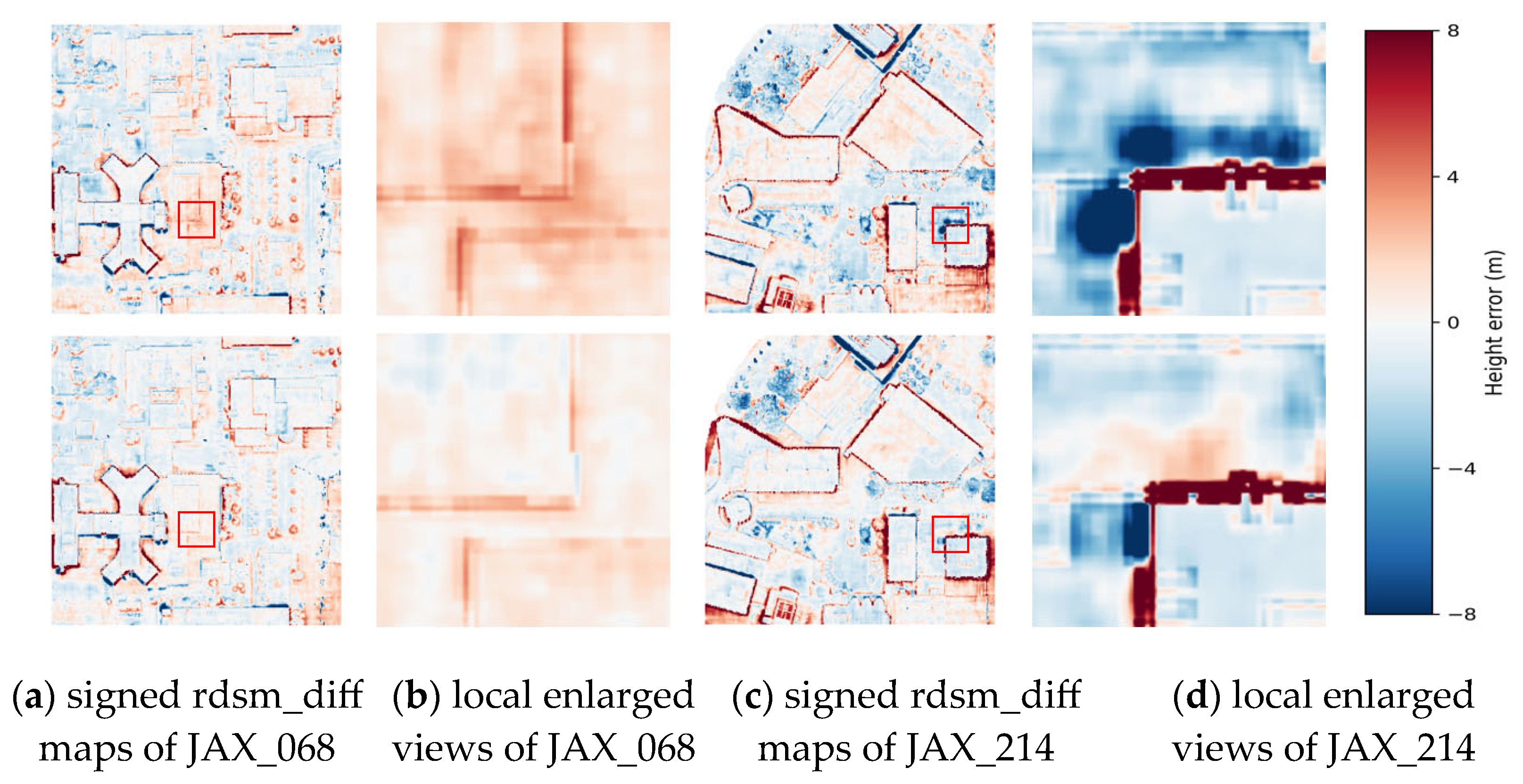
The results in Section 3 show consistent gains from SGC across backbones, but the mechanism is better understood when quantitative and qualitative evidence are read together. This section therefore interprets the supplementary metrics in

Table 6. Mean supplementary metrics over the eight RGB scenes for Sat-NeRF and EO-NeRF and their SGC-enhanced variants. Lower RE, Boundary-MAE, and Boundary-RMSE indicate better performance; higher completeness, correctness, and F1@$\tau$ indicate more reliable reconstruction within the specified error tolerance. The symbol ‘↑’ indicates higher values are better, while ‘↓’ indicates lower values are better.

Method	RE ↓	Completeness ↑	Correctness ↑	F1@τ ↑	Boundary-MAE ↓	Boundary-RMSE ↓
SAT-NERF	11.024	0.453	0.460	0.457	2.217	3.489
SAT-NERF+SGC	9.255	0.508	0.517	0.513	2.130	3.395
EO-NERF	9.956	0.412	0.489	0.436	2.422	3.699
EO-NERF+SGC	8.053	0.500	0.585	0.527	2.109	3.351

, analyzes spatial error patterns in Figure 13, and discusses the PIM decomposition evidence in Figure 14. The emphasis is not only on average improvement, but also on where gains are concentrated and where residual errors remain.

4.1. Interpretation of the Supplementary Metrics

Beyond the scene-wise MAE and RMSE in Table 2, Table 6 reports the mean supplementary metrics over the eight RGB scenes for Sat-NeRF and EO-NeRF, with and without SGC. These metrics complement global error: RE normalizes height error by scene relief, completeness, and correctness characterize tolerance-level consistency, F1@$\tau$ balances the two, and Boundary-MAE/Boundary-RMSE focus on edge-sensitive regions where urban DSM reconstruction is typically most difficult.

As shown in Table 6, SGC improves all supplementary metrics for both backbones. For Sat-NeRF, RE decreases from 11.024 to 9.255, and F1@$\tau$ increases from 0.457 to 0.513; for EO-NeRF, RE decreases from 9.956 to 8.053, and F1@$\tau$ increases from 0.436 to 0.527. Boundary-MAE and Boundary-RMSE also decrease for both models, indicating that the gain is not limited to global averages but extends to boundary-critical regions.

4.2. Spatial Error Analysis in Boundary and Vegetation Regions

Average metrics indicate overall improvement, but they do not reveal where residual errors are concentrated. We therefore analyze two complementary cases: boundary-dominant urban regions and vegetation-heavy regions. Figure 13 first compares signed rdsm_diff maps and local enlargements for EO-NeRF and EO-NeRF+SGC in two representative urban scenes, JAX_068 and JAX_214. To extend the analysis beyond building-boundary regions, we additionally evaluate vegetation and non-vegetation MAE in JAX_004 and JAX_260 using binary region masks. All heat maps are rendered with the same fixed color scale [−8, +8] m, enabling direct visual comparison of error intensity and spatial distribution. Under this fixed display range, a small number of localized boundary outliers can remain visually salient even when the scene-wide MAE decreases.

In JAX_068, the baseline already captures the main urban layout, but residual errors remain around roof boundaries, roof-to-ground transitions, and concave structural corners. After adding SGC, several roof and ground regions become less diffuse in the error map, and the enlarged views show tighter boundary-localized responses. This pattern agrees with the boundary-metric improvements reported in Table 6.

JAX_214 shows a complementary behavior: EO-NeRF+SGC regularizes broad planar regions and suppresses part of scattered high-error responses, while thin residual strips persist near sharp edges and complex transitions.

Whereas the JAX_068 and JAX_214 examples emphasize boundary-localized urban errors, vegetation-heavy scenes require a different diagnostic because their dominant errors are less confined to straight building boundaries. Using binary vegetation masks on JAX_004 and JAX_260, we separately computed MAE over vegetation and non-vegetation regions from the registered DSM outputs. EO-NeRF+SGC reduces the vegetation/non-vegetation MAE from 2.856/0.909 m to 2.795/0.842 m in JAX_004 and from 2.598/1.378 m to 2.166/1.097 m in JAX_260, corresponding to relative reductions of 2.13%/7.28% and 16.61%/20.39%, respectively. These results show that SGC improves not only rigid urban structures but also more irregular vegetated areas, although the residual errors remain larger over vegetation than over surrounding non-vegetated surfaces. This gap is consistent with the non-rigid canopy structure, weaker multi-view consistency on thin branches and crowns, and locally unstable depth support under self-occlusion. Therefore, the strongest and most localized gains still appear around regular urban boundaries, whereas in vegetation-heavy scenes, SGC delivers broader but less spatially concentrated error reduction.

4.3. Role of the Physical Imaging Model: Albedo and Shading Decomposition

Figure 14 provides mechanism-oriented evidence for the role of the physical imaging model in shadowed urban reconstruction. In JAX_068, the estimated albedo maps are more uniform across roofs and roads than the raw RGB observations, while the mean-ratio shading maps isolate the dominant illumination-loss pattern. This separation helps decouple reflectance from lighting and reduces shadow-driven ambiguity during geometry optimization.

The paired views show that corresponding structures retain similar albedo despite clear brightness changes in the original images, indicating that illumination variation is largely absorbed by the shading component rather than encoded as false reflectance change.

The normal maps offer a geometric consistency check: major roof planes and transition areas remain coherent after introducing PIM, which supports stable optimization near boundaries and shaded facades.

These qualitative results should be interpreted as explanatory evidence rather than a strict inverse-rendering benchmark, because this dataset provides no ground-truth albedo, shading, or normals. Accordingly, Figure 14 is used to explain why PIM helps geometric reconstruction under shadows, not to claim fully accurate physical decomposition for all materials and conditions.

4.4. Efficiency and Practical Applicability

To assess the engineering practicality of the proposed module, we report the average training time required to reach convergence over the four NEW scenes used in the main EO-NeRF comparison, namely JAX_004, JAX_068, JAX_214, and JAX_260. Based on these experiments, EO-NeRF requires about 2.6 h on average to converge, whereas EO-NeRF+SGC requires about 8.2 h.

Although SGC increases the convergence-time cost during training, the GPU memory overhead remains very small. In the profiled reference run, peak GPU memory stays nearly unchanged after introducing SGC, remaining at about 9.30–9.33 GiB. Therefore, the main computational cost of SGC lies in additional optimization time rather than in substantially higher memory usage.

The inference-stage overhead is much smaller. When rendering three validation images from JAX_068, the baseline requires 6.69 s per image on average (24,549 rays/s) with 0.69 GiB peak allocated GPU memory, while EO-NeRF+SGC requires 6.73 s per image (24,378 rays/s) with 0.68 GiB. This near-identical test-time behavior indicates that the additional cost of SGC is concentrated in training, whereas inference remains essentially unchanged. From an application perspective, such a trade-off is acceptable for offline DSM reconstruction, where improved geometric fidelity around boundaries, shadowed roofs, and complex urban transitions is often more important than minimizing training time.

To provide a first controlled check of image-count robustness, we additionally conducted a reduced-view experiment on OMA_203 RGB using the same rdsm_diff-based MAE criterion as in Table 2 and focusing on the near-nadir evaluation image OMA_203_010_RGB. With 15 training images, the MAE decreased from 1.840 m for EO-NeRF to 1.788 m for EO-NeRF+SGC. With 24 training images, the MAE decreased from 1.701 m for EO-NeRF to 1.654 m for EO-NeRF+SGC. These preliminary results indicate that SGC remains beneficial under reduced-image settings.

5. Conclusions

In this paper, we propose the Shading and Geometric Constraint (SGC), a general enhancement module for multi-view satellite NeRF-based DSM reconstruction.

The main theoretical contribution is a unified optimization formulation that couples a spherical-harmonics physical imaging model with edge-aware geometric regularization inside the NeRF training objective. This design links radiometric decomposition, shadow-robust supervision, and local surface-consistency priors, providing a physically grounded route to improve geometry rather than relying only on post-reconstruction refinement.

Across diverse scene types and two representative backbones, SGC consistently improves global elevation accuracy as well as boundary-sensitive quality. The results indicate that the radiometric component is especially helpful under radiance inconsistency and shadow, whereas the geometric component sharpens contours and stabilizes smooth structural regions.

The present study mainly evaluates DSM elevation accuracy and spatial error structure. A systematic benchmark of derived terrain parameters such as slope, roughness, curvature, and hillshade would also be valuable for downstream applications, but this lies beyond the current scope and remains an important direction for future work. To facilitate such follow-up analysis, the GeoTIFF elevation grids used in this study have been publicly released.

Remaining difficulties are concentrated in vegetation-dominated and highly non-Lambertian areas, where static-scene assumptions and appearance-guided regularization become less reliable. Future work will therefore focus on richer reflectance modeling, more efficient implementations, and stronger geometric priors for large-scale remote-sensing DSM reconstruction.

References

1. Mao, Y.; Chen, K.; Zhao, L.; Chen, W.; Tang, D.; Liu, W.; Wang, Z.; Diao, W.; Sun, X.; Fu, K. Elevation estimation-driven building 3-D reconstruction from single-view remote sensing imagery. IEEE Trans. Geosci. Remote Sens. 2023, 61, 5608718. [Google Scholar] [CrossRef]
2. Somanath, S.; Naserentin, V.; Eleftheriou, O.; Sjölie, D.; Wästberg, B.S.; Logg, A. Towards urban digital twins: A workflow for procedural visualization using geospatial data. Remote Sens. 2024, 16, 1939. [Google Scholar] [CrossRef]
3. Behari, N.; Dave, A.; Tiwary, K.; Yang, W.; Raskar, R. SUNDIAL: 3D Satellite Understanding through Direct Ambient and Complex Lighting Decomposition. In Proceedings of the IEEE/CVF CVPR, Seattle, WA, USA, 17–21 June 2024; pp. 522–532. [Google Scholar] [CrossRef]
4. Wang, Y.; Dong, P.; Liao, S.; Zhu, Y.; Zhang, D.; Yin, N. Urban Expansion Monitoring Based on the Digital Surface Model—A Case Study of the Beijing–Tianjin–Hebei Plain. Appl. Sci. 2022, 12, 5312. [Google Scholar] [CrossRef]
5. Zhou, S.; Mi, L.; Chen, H.; Geng, Y. Building detection in Digital Surface Model. In Proceedings of the IEEE International Conference on Imaging Systems and Techniques (IST), Beijing, China, 22–23 October 2013; pp. 194–199. [Google Scholar] [CrossRef]
6. Mei, G.; Tipper, J.C.; Xu, N. Discrete surface modeling based on Google Earth: A case study. In Proceedings of the IEEE International Conference on Computer Science and Network Technology (ICCSNT), Changchun, China, 29–31 December 2012; pp. 1137–1141. [Google Scholar] [CrossRef]
7. Jenkins, L.T.; Creed, M.J.; Tarbali, K.; Muthusamy, M.; Trogrlić, R.Š.; Phillips, J.C.; Watson, C.S.; Sinclair, H.D.; Galasso, C.; McCloskey, J. Physics-based simulations of multiple natural hazards for risk-sensitive planning and decision making in expanding urban regions. Int. J. Disaster Risk Reduct. 2023, 84, 103460. [Google Scholar] [CrossRef]
8. Chen, L.C.; Teo, T.A.; Shao, Y.C.; Lai, Y.-C.; Rau, J.-Y. Fusion of LIDAR data and optical imagery for building modeling. Int. Arch. Photogramm. Remote Sens. 2004, 35, 732–737. [Google Scholar]
9. Han, Y.; Wang, S.; Gong, D.; Wang, Y.; Ma, X. State of the art in digital surface modelling from multi-view high-resolution satellite images. ISPRS Ann. Photogramm. Remote Sens. Spat. Inf. Sci. 2020, 2, 351–356. [Google Scholar] [CrossRef]
10. Serati, G.; Sedaghat, A.; Mohammadi, N.; Li, J. Digital surface model generation from high-resolution satellite stereo imagery based on structural similarity. Geocarto Int. 2022, 37, 11390–11419. [Google Scholar] [CrossRef]
11. Hirschmuller, H. Stereo Processing by Semiglobal Matching and Mutual Information. IEEE Trans. Pattern Anal. Mach. Intell. 2008, 30, 328–341. [Google Scholar] [CrossRef]
12. Furukawa, Y.; Ponce, J. Accurate, Dense, and Robust Multiview Stereopsis. IEEE Trans. Pattern Anal. Mach. Intell. 2010, 32, 1362–1376. [Google Scholar] [CrossRef] [PubMed]
13. Vu, H.; Labatut, P.; Pons, J.; Keriven, R. High Accuracy and Visibility-Consistent Dense Multiview Stereo. IEEE Trans. Pattern Anal. Mach. Intell. 2011, 34, 889–901. [Google Scholar] [CrossRef]
14. Schönberger, J.; Hardmeier, H.; Sattler, T.; Pollefeys, M. Comparative Evaluation of Hand-Crafted and Learned Local Features. In Proceedings of the IEEE/CVF CVPR, Honolulu, HI, USA, 21–26 July 2017; pp. 6959–6968. [Google Scholar] [CrossRef]
15. Yao, Y.; Luo, Z.; Li, S.; Fang, T.; Quan, L. MVSNet: Depth Inference for Unstructured Multi-view Stereo. In Proceedings of the ECCV, Munich, Germany, 8–14 September 2018; pp. 767–783. [Google Scholar] [CrossRef]
16. Yi, H.; Wei, Z.; Ding, M.; Zhang, R.; Chen, Y.; Wang, G.; Tai, Y.-W. Pyramid Multi-view Stereo Net with Self-adaptive View Aggregation. In Proceedings of the ECCV, Glasgow, UK, 23–28 August 2020; pp. 766–782. [Google Scholar] [CrossRef]
17. Zhao, Y.; Liu, Y.; Gao, S.; Liu, G.; Wan, Z.; Hu, D. Deep learning-based digital surface model reconstruction of ZY-3 satellite imagery. Remote Sens. 2024, 16, 2567. [Google Scholar] [CrossRef]
18. Mildenhall, B.; Srinivasan, P.P.; Tancik, M.; Barron, J.T.; Ramamoorthi, R.; Ng, R. NeRF: Representing scenes as neural radiance fields for view synthesis. Commun. ACM 2021, 65, 99–106. [Google Scholar] [CrossRef]
19. Gao, K.; Gao, Y.; He, H.; Lu, D.; Xu, L.; Li, J. NeRF: Neural radiance field in 3d vision, a comprehensive review. arXiv 2022, arXiv:2210.00379. [Google Scholar]
20. Yao, M.; Huo, Y.; Ran, Y.; Tian, Q.; Wang, R.; Wang, H. Neural radiance field-based visual rendering: A comprehensive review. arXiv 2024, arXiv:2404.00714. [Google Scholar] [CrossRef]
21. Ma, Q.; Paudel, D.P.; Chhatkuli, A.; Gool, L.V. Deformable neural radiance fields using rgb and event cameras. In Proceedings of the IEEE ICCV, Paris, France, 2–6 October 2023; pp. 3590–3600. [Google Scholar] [CrossRef]
22. Park, K.; Sinha, U.; Barron, J.T.; Bouaziz, S.; Goldman, D.B.; Seitz, S.M.; Martin-Brualla, R. NeRFies: Deformable neural radiance fields. In Proceedings of the IEEE ICCV, Montreal, QC, Canada, 11–17 October 2021; pp. 5865–5874. [Google Scholar] [CrossRef]
23. Pumarola, A.; Corona, E.; Pons-Moll, G.; Moreno-Noguer, F. D-NeRF: Neural radiance fields for dynamic scenes. In Proceedings of the IEEE/CVF CVPR, Nashville, TN, USA, 20–25 June 2021; pp. 10318–10327. [Google Scholar] [CrossRef]
24. Huang, X.; Zhang, Q.; Feng, Y.; Li, H.; Wang, X.; Wang, Q. Hdr-nerf: High dynamic range neural radiance fields. In Proceedings of the IEEE/CVF CVPR, New Orleans, LA, USA, 18–24 June 2022; pp. 18398–18408. [Google Scholar] [CrossRef]
25. Mildenhall, B.; Hedman, P.; Martin-Brualla, R.; Srinivasan, P.; Barron, J.T. Nerf in the dark: High dynamic range view synthesis from noisy raw images. In Proceedings of the IEEE/CVF CVPR, New Orleans, LA, USA, 18–24 June 2022; pp. 16190–16199. [Google Scholar] [CrossRef]
26. Korhonen, J.; Rangu, G.; Tavakoli, H.R.; Kannala, J. Efficient NeRF Optimization-Not All Samples Remain Equally Hard. In Proceedings of the ECCV, Milan, Italy, 29 September–4 October 2024; pp. 198–213. [Google Scholar] [CrossRef]
27. Deng, C.L.; Tartaglione, E. Compressing explicit voxel grid representations: Fast NeRFs become also small. In Proceedings of the IEEE WACV, Waikoloa, HI, USA, 2–7 January 2023; pp. 1236–1245. [Google Scholar] [CrossRef]
28. Deng, K.; Liu, A.; Zhu, J.Y.; Deva, R. Depth-supervised NeRF: Fewer views and faster training for free. In Proceedings of the IEEE/CVF CVPR, New Orleans, LA, USA, 18–24 June 2022; pp. 12882–12891. [Google Scholar] [CrossRef]
29. Martin-Brualla, R.; Radwan, N.; Sajjadi, M.S.M.; Barron, J.T.; Dosovitskiy, A.; Duckworth, D. NeRF in the wild: Neural radiance fields for unconstrained photo collections. In Proceedings of the IEEE/CVF CVPR, Nashville, TN, USA, 20–25 June 2021; pp. 7210–7219. [Google Scholar] [CrossRef]
30. Derksen, D.; Izzo, D. Shadow neural radiance fields for multi-view satellite photogrammetry. In Proceedings of the IEEE/CVF CVPR, Nashville, TN, USA, 20–25 June 2021; pp. 1152–1161. [Google Scholar] [CrossRef]
31. Wei, P.; Yan, L.; Xie, H.; Qiu, D.; Qiu, C.; Wu, H.; Zhao, Y.; Hu, X.; Huang, M. LiDeNeRF: Neural radiance field reconstruction with depth prior provided by LiDAR point cloud. ISPRS J. Photogramm. Remote Sens. 2024, 208, 296–307. [Google Scholar] [CrossRef]
32. Guo, S.; Wang, Q.; Gao, Y.; Xie, R.; Li, L.; Zhu, F.; Song, L. Depth-guided robust point cloud fusion NeRF for sparse input views. IEEE Trans. Circuits Syst. Video Technol. 2024, 34, 8093–8106. [Google Scholar] [CrossRef]
33. Marí, R.; Facciolo, G.; Ehret, T. Sat-NeRF: Learning multi-view satellite photogrammetry with transient objects and shadow modeling using rpc cameras. In Proceedings of the IEEE/CVF CVPR, New Orleans, LA, USA, 18–24 June 2022; pp. 1311–1321. [Google Scholar] [CrossRef]
34. Li, P.; Wang, S.; Yang, C.; Liu, B.; Qiu, W.; Wang, H. NeRF-MS: Neural radiance fields with multi-sequence. In Proceedings of the IEEE/CVF ICCV, Paris, France, 2–6 October 2023; pp. 18591–18600. [Google Scholar] [CrossRef]
35. Han, J.; Cavalheiro, G.; Biberstein, J.; Alkabawi, E.; Alqhatni, S.; Alaskar, F.; Bin Khunayn, E.; Karaman, S. CaLiSa-NeRF: Neural Radiance Field with Pinhole Camera Images LiDAR point clouds and Satellite Imagery for Urban Scene Representation. In Proceedings of the WACV, Tucson, AZ, USA, 28 February–4 March 2025; pp. 442–450. [Google Scholar] [CrossRef]
36. Marí, R.; Facciolo, G.; Ehret, T. Multi-date earth observation NeRF: The detail is in the shadows. In Proceedings of the IEEE/CVF CVPR, Vancouver, BC, Canada, 17–24 June 2023; pp. 2035–2045. [Google Scholar] [CrossRef]
37. Horn, B.K.P. Shape from Shading: A Method for Obtaining the Shape of a Smooth Opaque Object from One View. Ph.D. Thesis, Massachusetts Institute of Technology, Cambridge, MA, USA, 1970; 232p. [Google Scholar]
38. Oren, M.; Nayar, S.K. Generalization of Lambert’s reflectance model. In Proceedings of the 21st Annual Conference on Computer Graphics and Interactive Technique, Orlando, FL, USA, 24–29 July 1994; pp. 239–246. [Google Scholar] [CrossRef]
39. Peng, J.; Zhang, Y.; Shan, J. Shading-based DEM refinement under a comprehensive imaging model. ISPRS J. Photogramm. Remote Sens. 2015, 110, 24–33. [Google Scholar] [CrossRef]
40. Wu, C.; Wilburn, B.; Matsushita, Y.; Theobalt, C. High-quality shape from multi-view stereo and shading under general illumination. In Proceedings of the IEEE/CVF CVPR, Colorado Springs, CO, USA, 20–25 June 2011; pp. 969–976. [Google Scholar] [CrossRef]
41. Hu, Z.; Zhang, K.; Liu, Y. Edge constrained DSM refinement based on shading from high resolution multi-view satellite images. IEEE J. Sel. Top. Appl. Earth Obs. Remote Sens. 2025, 18, 5244–5254. [Google Scholar] [CrossRef]
42. Hu, Z.; Hou, Y.; Tao, P.; Shan, J. SREVAS: Shading Based Surface Refinement under Varying Albedo and Specularity. Remote Sens. 2020, 12, 3488. [Google Scholar] [CrossRef]
43. He, K.; Sun, J.; Tang, X. Guided image filtering. IEEE Trans. Pattern Anal. Mach. Intell. 2013, 35, 1397–1409. [Google Scholar] [CrossRef]
44. Zhang, W.; Deng, B.; Zhang, J.; Bouaziz, S.; Liu, L. Guided mesh normal filtering. Comput. Graph. Forum 2015, 34, 23–34. [Google Scholar] [CrossRef]
45. Heise, P.; Jensen, B.; Klose, S.; Knoll, A. Variational patchmatch multiview reconstruction and refinement. In Proceedings of the IEEE ICCV, Santiago, Chile, 7–13 December 2015; pp. 882–890. [Google Scholar] [CrossRef]
46. Savant, A.L.; Facciolo, G.; Ehret, T. Gaussian Splatting for Efficient Satellite Image Photogrammetry. In Proceedings of the IEEE/CVF CVPR, Seattle, WA, USA, 17–21 June 2025; pp. 5959–5969. [Google Scholar] [CrossRef]
Figure 1. Overall process of the proposed method. Besides the Vanilla NeRF rendering pipeline, we additionally introduced a physical imaging process under the Lambertian reflectance model represented by spherical harmonics. Furthermore, a geometric constraint using normal vector smoothing loss is also introduced.
Remotesensing 18 01091 g001
Figure 2. Schematic of the physical imaging model based on spherical harmonics. Direct sunlight and ambient skylight jointly determine the incident irradiance. For a surface point P, the synthesized intensity is computed from illumination, normal, albedo, and shadow, and is used as auxiliary supervision during NeRF training.
Remotesensing 18 01091 g002
Figure 3. Illustration of the proposed geometric structure constraints. Left: adaptive normal smoothness guided by photometric similarity. Right: bilateral edge-aware geometric refinement on the tangent plane, which suppresses local noise while preserving structural discontinuities.
Remotesensing 18 01091 g003
Figure 4. Typical examples from the selected regions.
Remotesensing 18 01091 g004
Figure 5. Details of the reconstruction model in Area JAX_068. (a) The RGB image, (b) the ground truth, (c) the result of Sat-NeRF, (d) the result of Sat-NeRF+SGC, (e) the result of EO-NeRF, and (f) the result of EO-NeRF+SGC. The second to fourth rows are the magnified details corresponding to the red boxes in the first row.
Remotesensing 18 01091 g005
Figure 6. Details of the reconstruction model in Area JAX_214. (a) The RGB image, (b) the ground truth, (c) the result of Sat-NeRF, (d) the result of Sat-NeRF+SGC, (e) the result of EO-NeRF, and (f) the result of EO-NeRF+SGC. The second to fourth rows are the magnified details corresponding to the red boxes in the first row.
Remotesensing 18 01091 g006
Figure 7. Details of the reconstruction model in Area JAX_004. (a) The RGB image, (b) the ground truth, (c) the result of Sat-NeRF, (d) the result of Sat-NeRF+SGC, (e) the result of EO-NeRF, and (f) the result of EO-NeRF+SGC. The second to fourth rows are the magnified details corresponding to the red boxes in the first row.
Remotesensing 18 01091 g007
Figure 8. Details of the reconstruction model in Area JAX_260. (a) The RGB image, (b) the ground truth, (c) the result of Sat-NeRF, (d) the result of Sat-NeRF+SGC, (e) the result of EO-NeRF, and (f) the result of EO-NeRF+SGC. The second to fourth rows are the magnified details corresponding to the red boxes in the first row.
Remotesensing 18 01091 g008
Figure 9. Details of the reconstruction model in Area JAX_207. (a) The RGB image, (b) the ground truth, (c) the result of Sat-NeRF, (d) the result of Sat-NeRF+SGC, (e) the result of EO-NeRF, and (f) the result of EO-NeRF+SGC. The second to fourth rows are the magnified details corresponding to the red boxes in the first row.
Remotesensing 18 01091 g009
Figure 10. Details of the reconstruction model in Area JAX_264. (a) The RGB image, (b) the ground truth, (c) the result of Sat-NeRF, (d) the result of Sat-NeRF+SGC, (e) the result of EO-NeRF, and (f) the result of EO-NeRF+SGC. The second to fourth rows are the magnified details corresponding to the red boxes in the first row.
Remotesensing 18 01091 g010
Figure 11. Details of the reconstruction model in Area OMA_203. (a) The RGB image, (b) the ground truth, (c) the result of Sat-NeRF, (d) the result of Sat-NeRF+SGC, (e) the result of EO-NeRF, and (f) the result of EO-NeRF+SGC. The second to fourth rows are the magnified details corresponding to the red boxes in the first row.
Remotesensing 18 01091 g011
Figure 12. Details of the reconstruction model in Area OMA_212. (a) The RGB image, (b) the ground truth, (c) the result of Sat-NeRF, (d) the result of Sat-NeRF+SGC, (e) the result of EO-NeRF, and (f) the result of EO-NeRF+SGC. The second to fourth rows are the magnified details corresponding to the red boxes in the first row.
Remotesensing 18 01091 g012
Figure 13. (a) The signed rdsm_diff maps of JAX_068, (b) the local enlarged views of JAX_068, (c) the signed rdsm_diff maps of JAX_214, and (d) the local enlarged views of JAX_214. The first rows are the results of EO-NeRF, the second rows are the results of EO-NeRF+SGC. Red and blue denote positive and negative elevation errors relative to the LiDAR DSM. All maps use the same color range [−8 m, +8 m] for fair cross-scene and cross-method comparison, and values outside this interval are clipped to the display limits.
Remotesensing 18 01091 g013
Figure 14. Representative PIM decomposition results for three validation views in JAX_068. (a) The albedo maps, (b) the mean-ratio shading maps computed as mean (RGB)/mean (albedo), and (c) the normal maps. The decomposition suppresses shadow contrast in albedo, isolates illumination attenuation in shading, and preserves coherent geometry in normals.
Remotesensing 18 01091 g014