Figure 1.
The comparison of our method with some state-of-the-art methods. The x-axis represents mAP50, and the y-axis represents mAP. Both metrics are better when higher, and the size of the bubble is proportional to the mAP value. Our method achieves the best performance on both metrics.
Figure 1.
The comparison of our method with some state-of-the-art methods. The x-axis represents mAP50, and the y-axis represents mAP. Both metrics are better when higher, and the size of the bubble is proportional to the mAP value. Our method achieves the best performance on both metrics.
Figure 2.
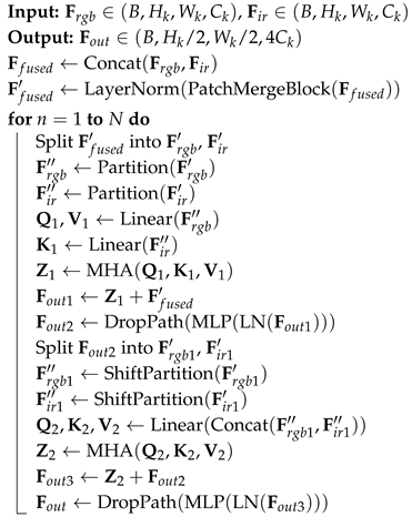
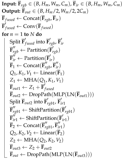
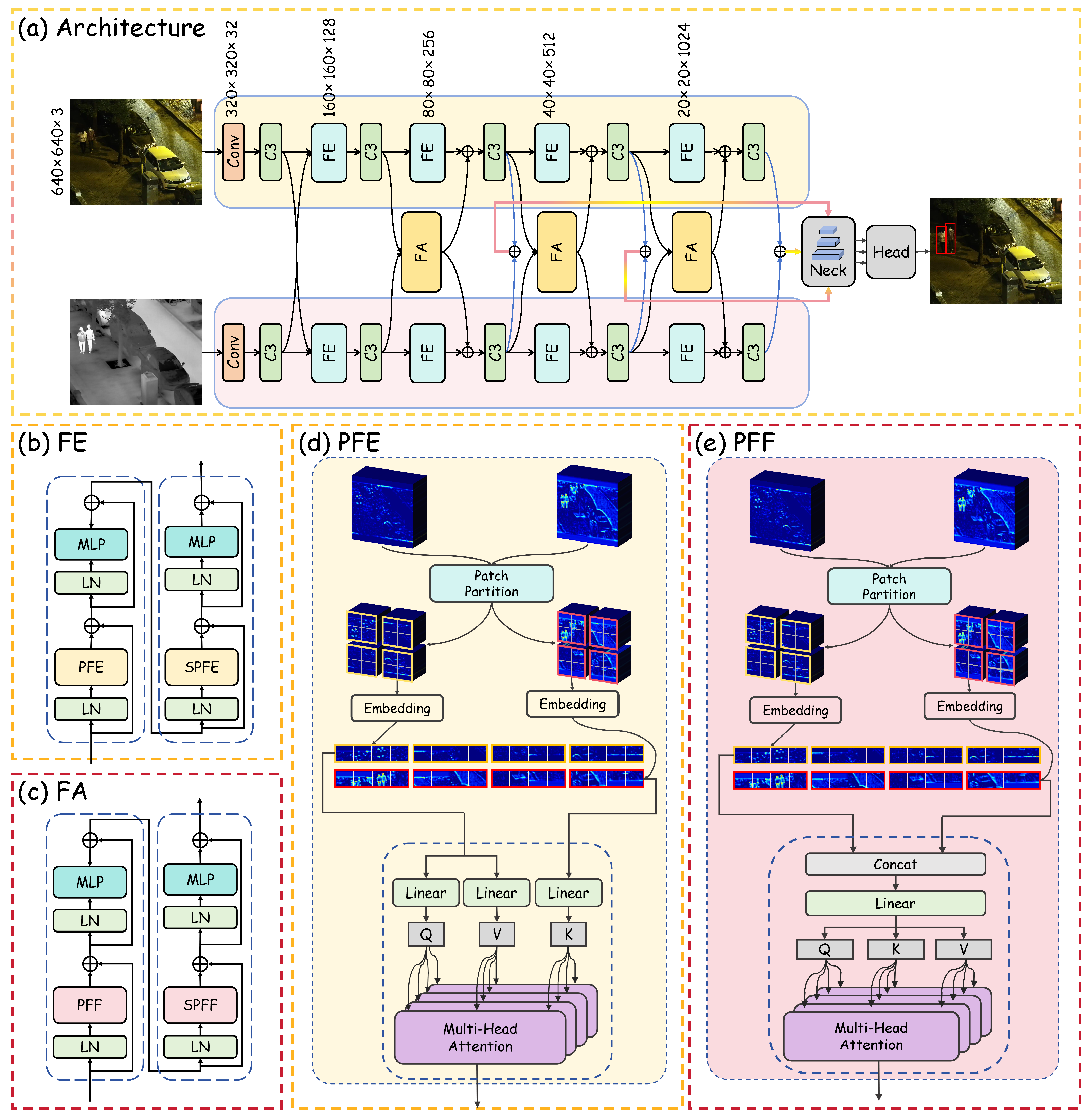
Overall architecture of the proposed multispectral object detection model. This end-to-end framework takes paired infrared and visible images as input and outputs object bounding boxes. The dual-stream backbone contains an infrared branch (structural cues) and a visible branch (texture cues). We introduce two Swin-style fusion modules: (a) architecture, the full dual-stream backbone with multi-scale feature extraction; (b) Feature Enhancer (FE) module, which achieves cross-modal feature alignment and enhancement through (d) patch-aware cross-modal feature enhancement (PFE) block and shifted-patch-aware cross-modal feature enhancement (SPFE) block; (c) Feature Aggregator (FA) module, which performs deep semantic fusion via (e) patch-aware unified fusion (PFF) block and shifted-patch-aware unified fusion (SPFF) block to integrate cross-modal information at the last three scales. Specifically, the shifted-patch strategy used in SPFE and SPFF is inherited from the Swin Transformer, facilitating efficient long-range dependency modeling.
Figure 2.
Overall architecture of the proposed multispectral object detection model. This end-to-end framework takes paired infrared and visible images as input and outputs object bounding boxes. The dual-stream backbone contains an infrared branch (structural cues) and a visible branch (texture cues). We introduce two Swin-style fusion modules: (a) architecture, the full dual-stream backbone with multi-scale feature extraction; (b) Feature Enhancer (FE) module, which achieves cross-modal feature alignment and enhancement through (d) patch-aware cross-modal feature enhancement (PFE) block and shifted-patch-aware cross-modal feature enhancement (SPFE) block; (c) Feature Aggregator (FA) module, which performs deep semantic fusion via (e) patch-aware unified fusion (PFF) block and shifted-patch-aware unified fusion (SPFF) block to integrate cross-modal information at the last three scales. Specifically, the shifted-patch strategy used in SPFE and SPFF is inherited from the Swin Transformer, facilitating efficient long-range dependency modeling.

Figure 3.
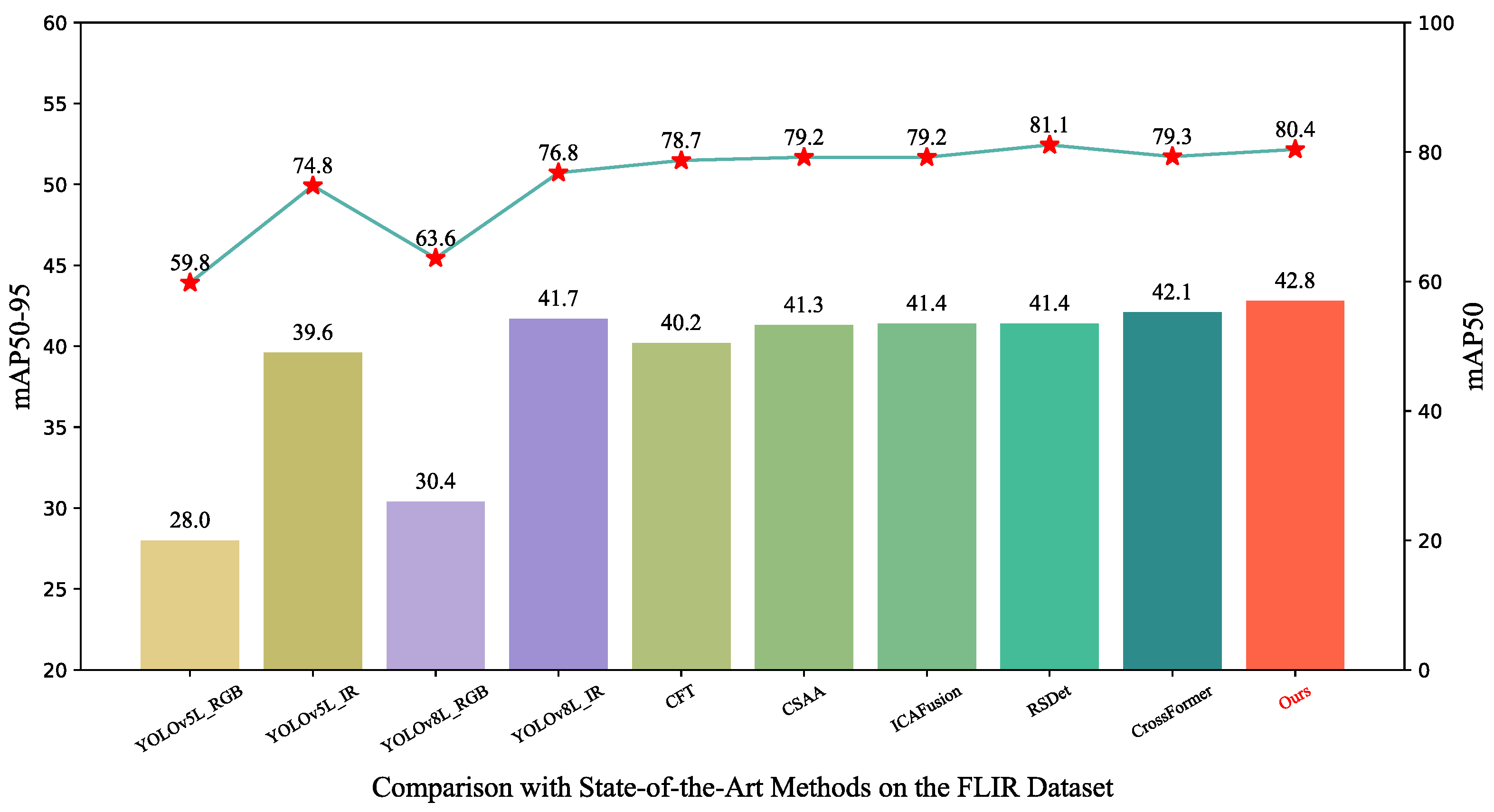
Performance comparison with state-of-the-art methods on the FLIR dataset. The bars represent mAP50-95 scores, while the red star markers indicate the corresponding mAP50 values for each method. Our method achieves the best performance with 42.8% mAP50-95 and 80.4% mAP50, demonstrating significant improvements over baseline methods, including single-modal (RGB/IR) and multi-modal fusion approaches.
Figure 3.
Performance comparison with state-of-the-art methods on the FLIR dataset. The bars represent mAP50-95 scores, while the red star markers indicate the corresponding mAP50 values for each method. Our method achieves the best performance with 42.8% mAP50-95 and 80.4% mAP50, demonstrating significant improvements over baseline methods, including single-modal (RGB/IR) and multi-modal fusion approaches.
Figure 4.
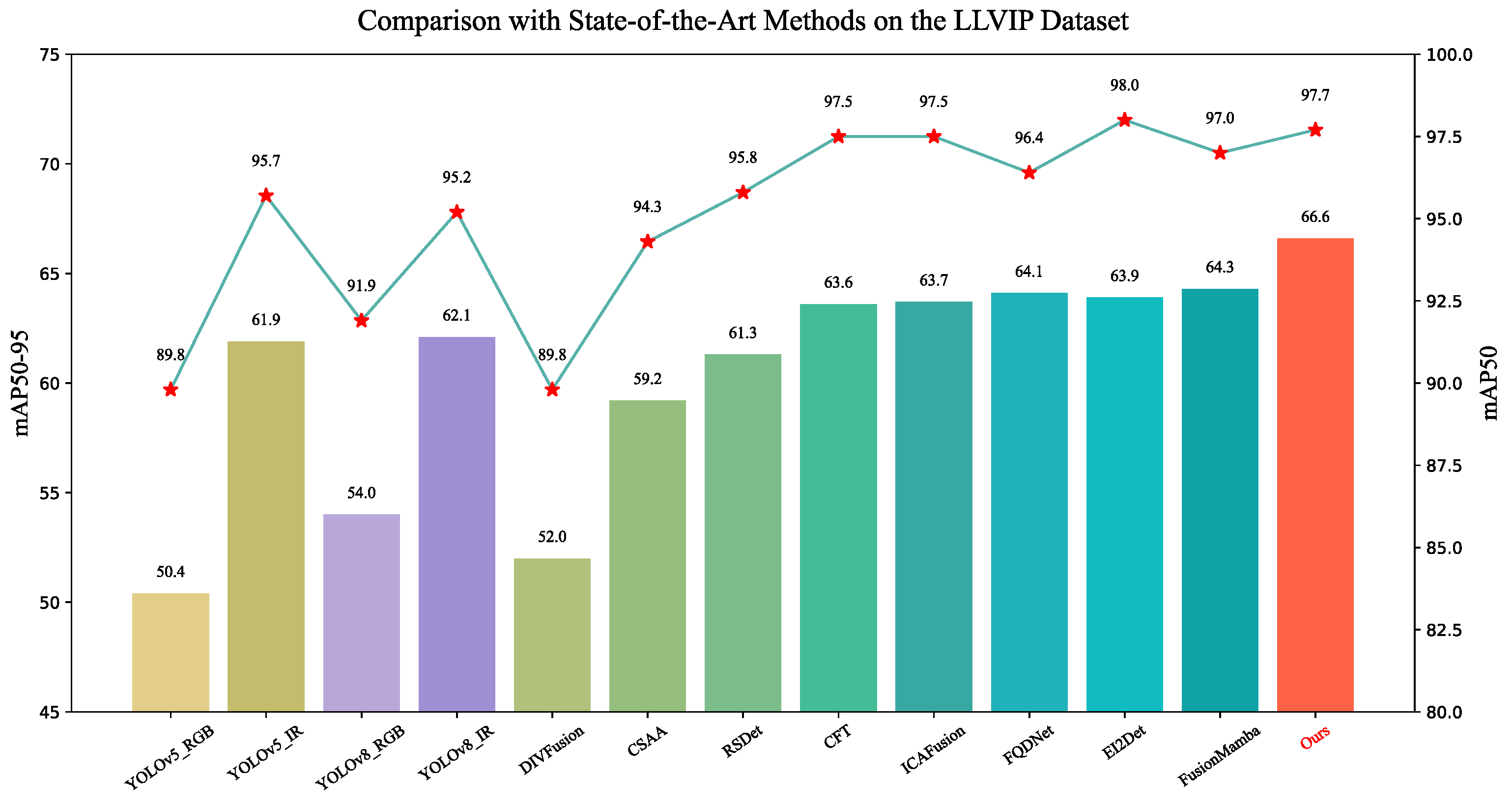
Performance comparison with state-of-the-art methods on the LLVIP dataset. The bars represent mAP50-95 scores, while the line with star markers indicates mAP50 scores. Our method achieves the highest performance on both metrics, demonstrating significant improvements over existing approaches.
Figure 4.
Performance comparison with state-of-the-art methods on the LLVIP dataset. The bars represent mAP50-95 scores, while the line with star markers indicates mAP50 scores. Our method achieves the highest performance on both metrics, demonstrating significant improvements over existing approaches.
Figure 5.
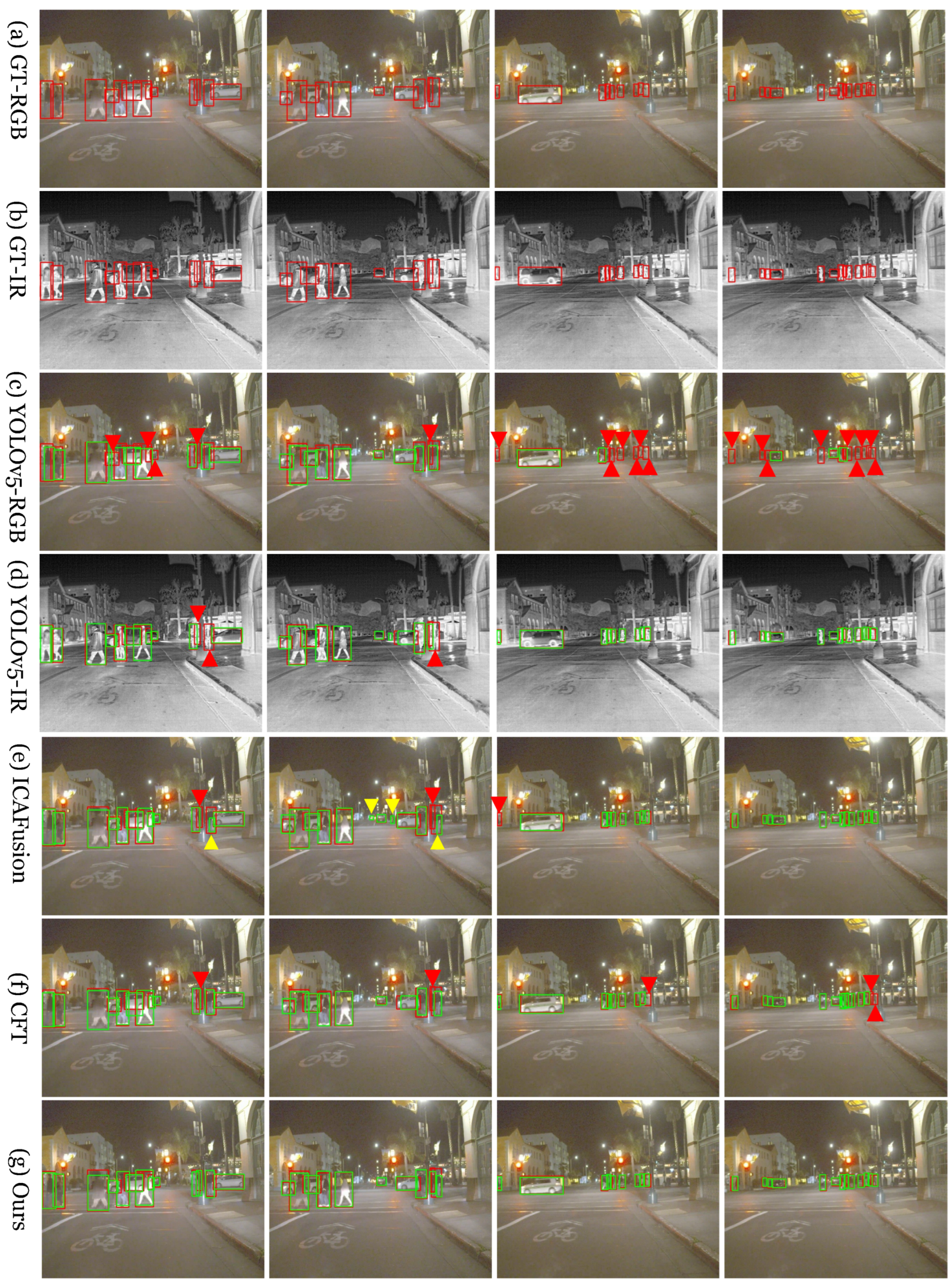
Qualitative comparison of our method with various benchmark methods on the FLIR dataset. The first and second rows show the RGB and infrared images annotated with GroundTruth. The third and fourth rows illustrate the detection results of the YOLOv5 method on RGB and IR images, respectively. The fifth and sixth rows represent the multispectral object detection results of the ICA and CFT methods. The last row shows the detection results of our method. Red bounding boxes indicate GroundTruth, while green boxes denote the detection results of each corresponding method. Red triangles indicate missed detections (miss), yellow triangles indicate false detections (false), and unmarked bounding boxes correspond to correct detections (true). Zoom in for more details.
Figure 5.
Qualitative comparison of our method with various benchmark methods on the FLIR dataset. The first and second rows show the RGB and infrared images annotated with GroundTruth. The third and fourth rows illustrate the detection results of the YOLOv5 method on RGB and IR images, respectively. The fifth and sixth rows represent the multispectral object detection results of the ICA and CFT methods. The last row shows the detection results of our method. Red bounding boxes indicate GroundTruth, while green boxes denote the detection results of each corresponding method. Red triangles indicate missed detections (miss), yellow triangles indicate false detections (false), and unmarked bounding boxes correspond to correct detections (true). Zoom in for more details.
Figure 6.
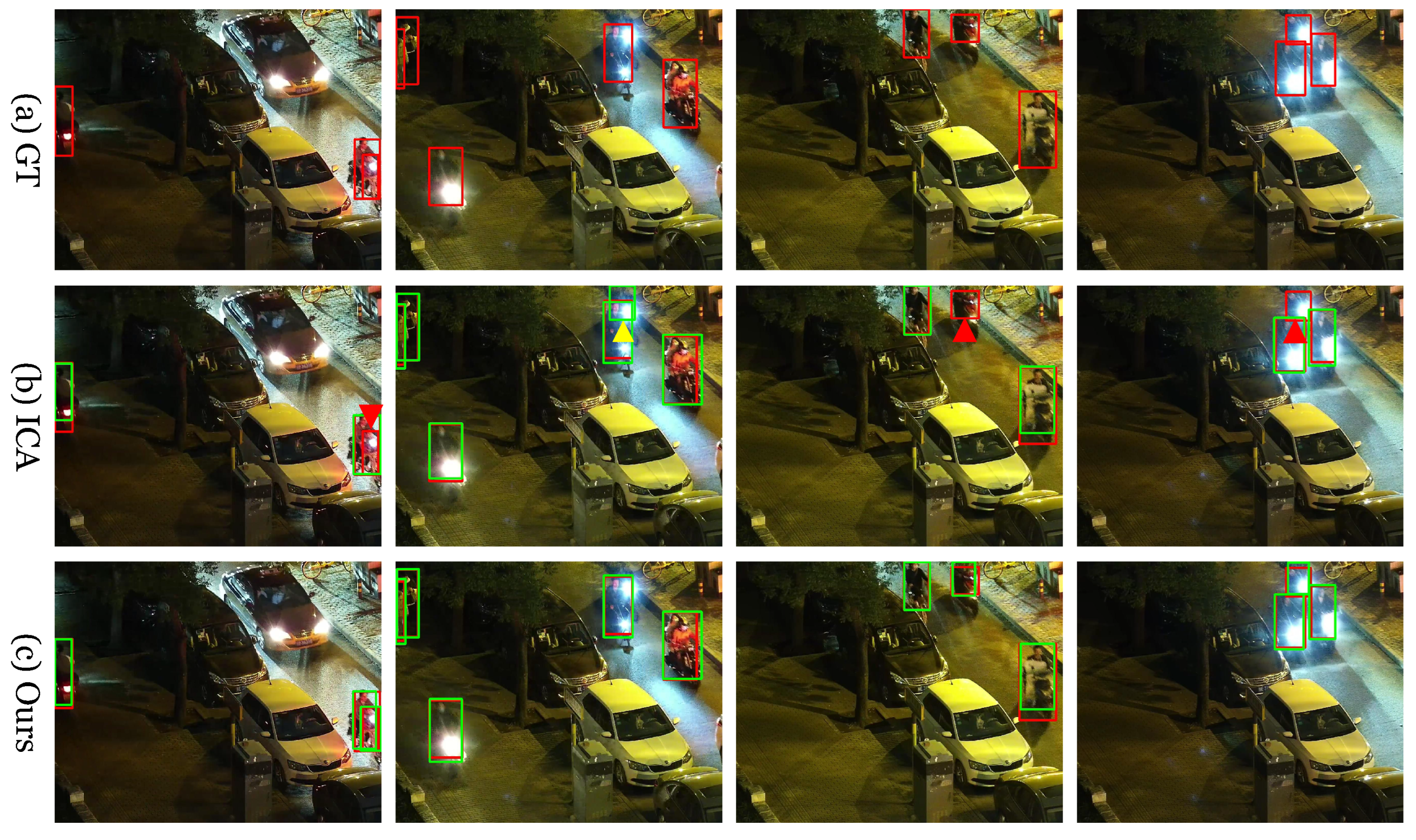
Qualitative comparison of our method with the ICA method on the LLVIP dataset. The first row shows the RGB images annotated with GroundTruth. The second row depicts the detection results of the ICA method, while the third row presents the detection results of our method. Red bounding boxes indicate GroundTruth, and green boxes denote the detection results of each corresponding method. Red triangles indicate missed detections (miss), yellow triangles indicate false detections (false), and unmarked bounding boxes correspond to correct detections (true).
Figure 6.
Qualitative comparison of our method with the ICA method on the LLVIP dataset. The first row shows the RGB images annotated with GroundTruth. The second row depicts the detection results of the ICA method, while the third row presents the detection results of our method. Red bounding boxes indicate GroundTruth, and green boxes denote the detection results of each corresponding method. Red triangles indicate missed detections (miss), yellow triangles indicate false detections (false), and unmarked bounding boxes correspond to correct detections (true).
Figure 7.
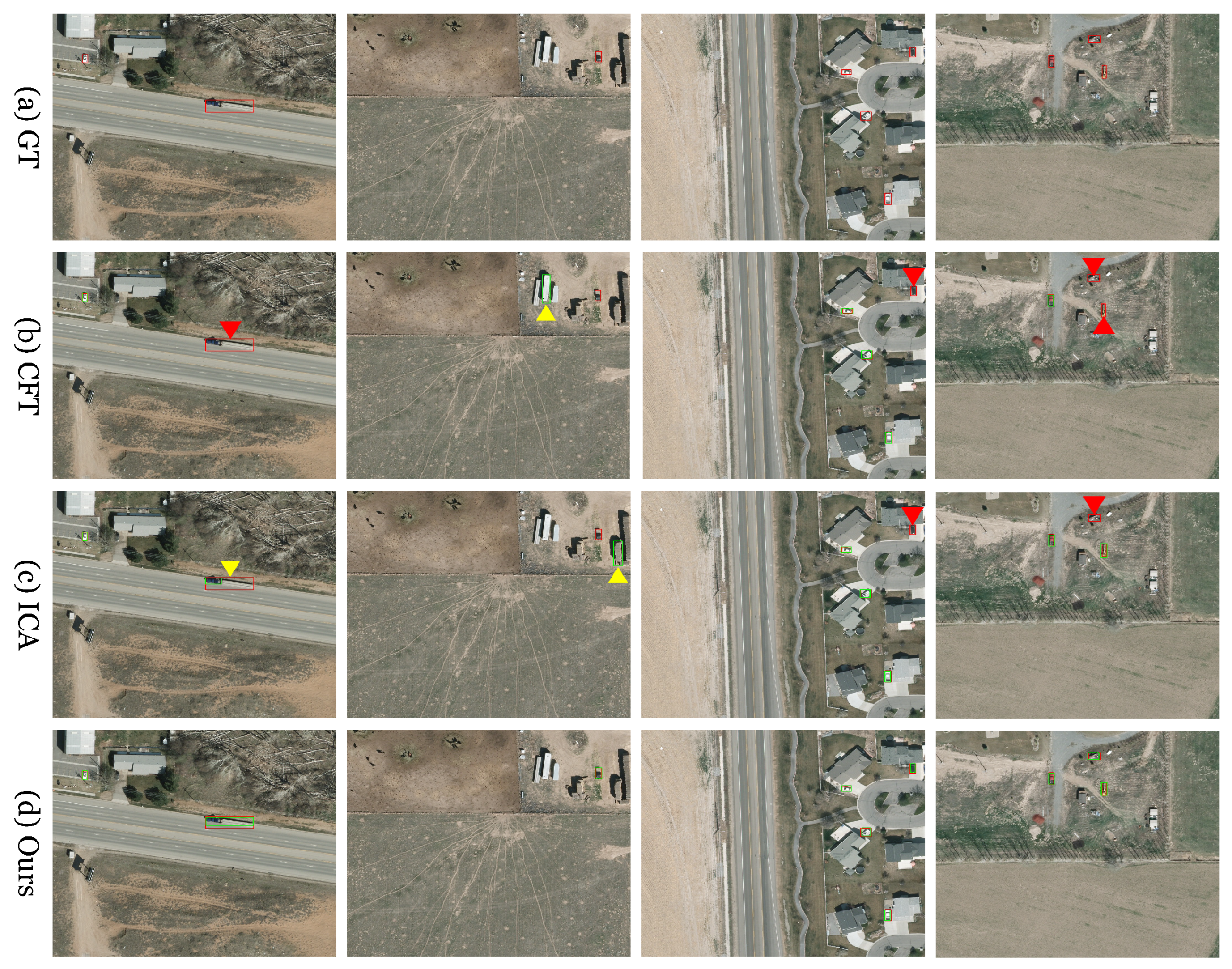
Qualitative comparison of our method with the CFT method on the LLVIP dataset. The first row shows the RGB images annotated with GroundTruth. The second row depicts the detection results of the CFT method, while the third row presents the detection results of our method. Red bounding boxes indicate GroundTruth, and green boxes denote the detection results of each corresponding method. Red triangles indicate missed detections (miss), and unmarked bounding boxes correspond to correct detections (true).
Figure 7.
Qualitative comparison of our method with the CFT method on the LLVIP dataset. The first row shows the RGB images annotated with GroundTruth. The second row depicts the detection results of the CFT method, while the third row presents the detection results of our method. Red bounding boxes indicate GroundTruth, and green boxes denote the detection results of each corresponding method. Red triangles indicate missed detections (miss), and unmarked bounding boxes correspond to correct detections (true).
Figure 8.
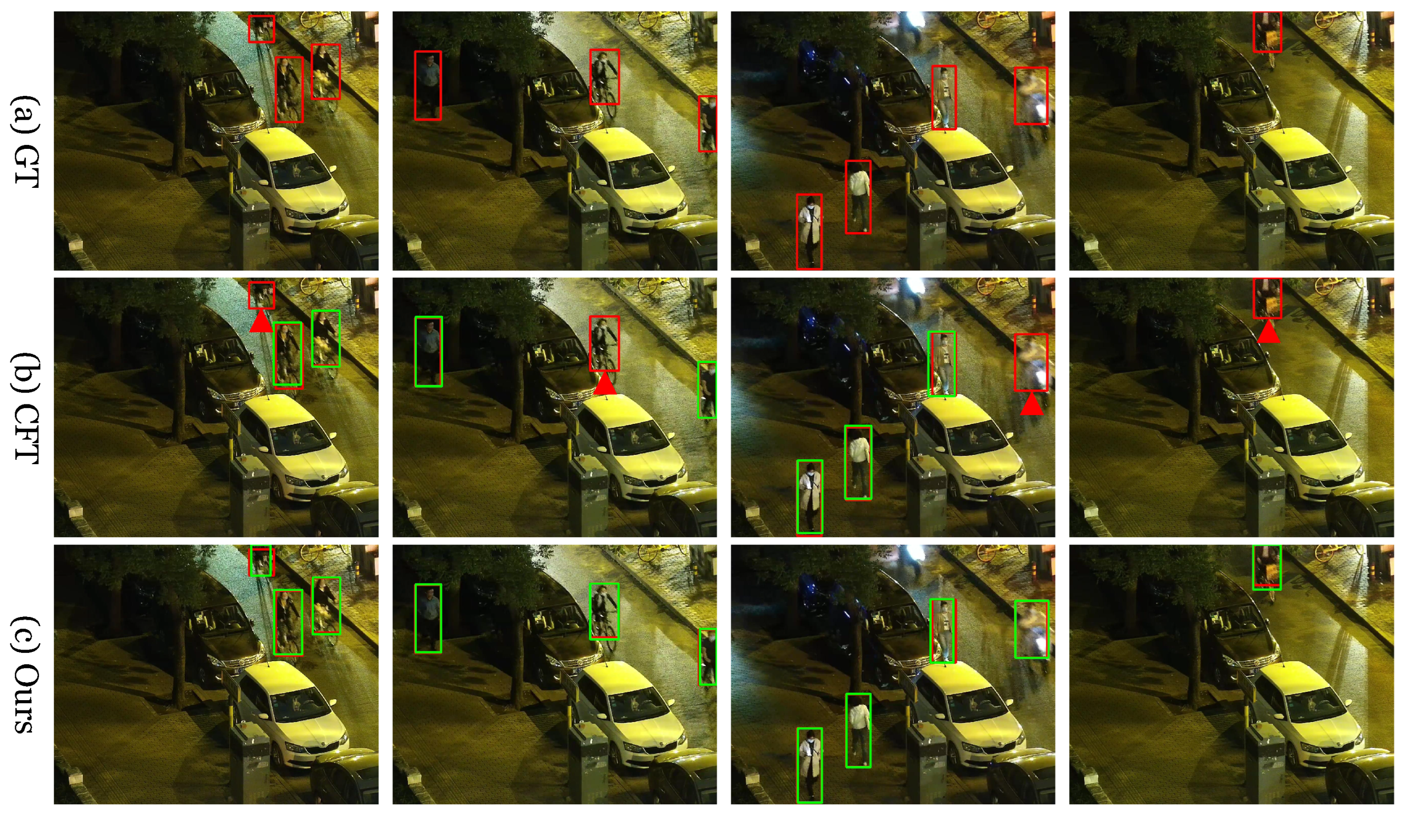
Qualitative comparison of multispectral object detection on the VEDAI dataset. The first row shows the RGB images annotated with GroundTruth. The second and third rows depict the detection results of the CFT and ICA methods, respectively, while the fourth row presents the detection results of our method. Red bounding boxes indicate GroundTruth, and green boxes denote the detection results of each corresponding method. Red triangles indicate missed detections (miss), yellow triangles indicate false detections (false), and unmarked bounding boxes correspond to correct detections (true).
Figure 8.
Qualitative comparison of multispectral object detection on the VEDAI dataset. The first row shows the RGB images annotated with GroundTruth. The second and third rows depict the detection results of the CFT and ICA methods, respectively, while the fourth row presents the detection results of our method. Red bounding boxes indicate GroundTruth, and green boxes denote the detection results of each corresponding method. Red triangles indicate missed detections (miss), yellow triangles indicate false detections (false), and unmarked bounding boxes correspond to correct detections (true).
Figure 9.
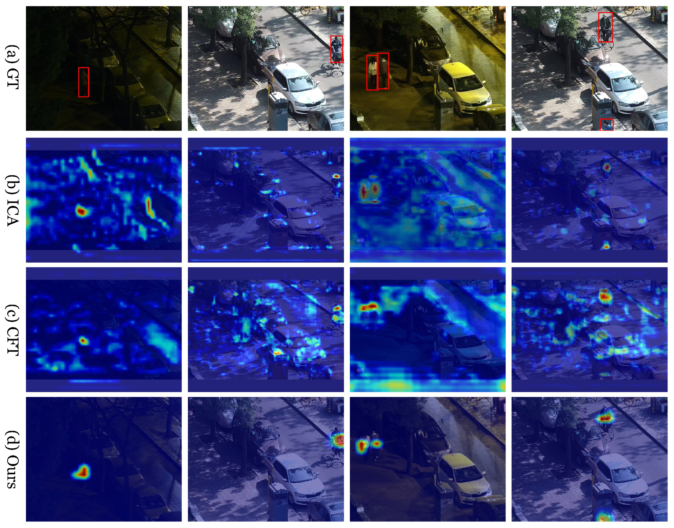
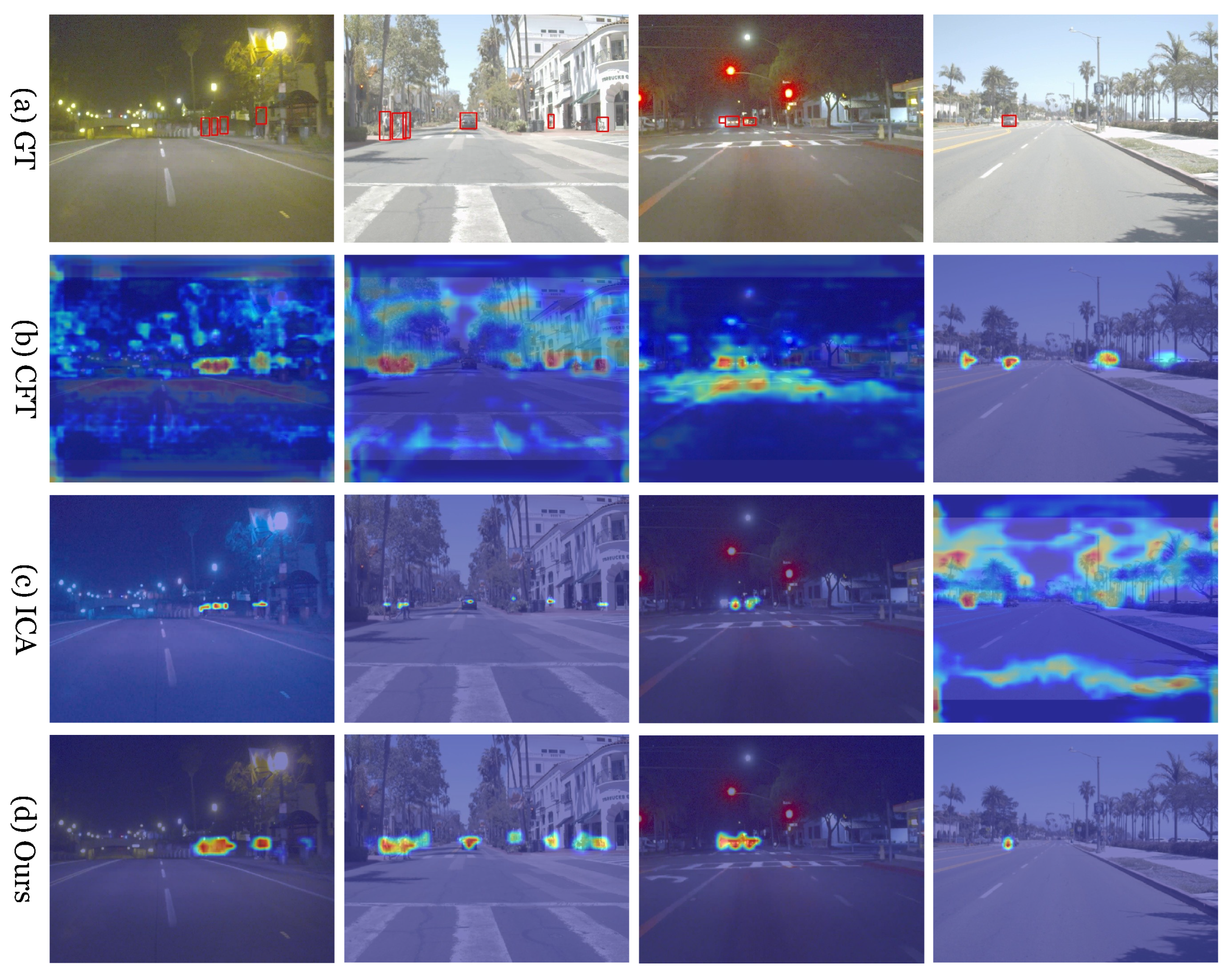
Heatmap visualization of various multimodal object detection methods on the FLIR dataset. The first row shows the RGB images annotated with GroundTruth. The second and third rows depict the heatmap visualization results of the CFT and ICA methods, respectively. The last row presents our heatmap visualization results. Red bounding boxes indicate GroundTruth. The color intensity in the heatmaps reflects the response strength, where warmer colors (e.g., red/yellow) denote higher responses and cooler colors (e.g., blue) indicate lower responses.
Figure 9.
Heatmap visualization of various multimodal object detection methods on the FLIR dataset. The first row shows the RGB images annotated with GroundTruth. The second and third rows depict the heatmap visualization results of the CFT and ICA methods, respectively. The last row presents our heatmap visualization results. Red bounding boxes indicate GroundTruth. The color intensity in the heatmaps reflects the response strength, where warmer colors (e.g., red/yellow) denote higher responses and cooler colors (e.g., blue) indicate lower responses.
Figure 10.
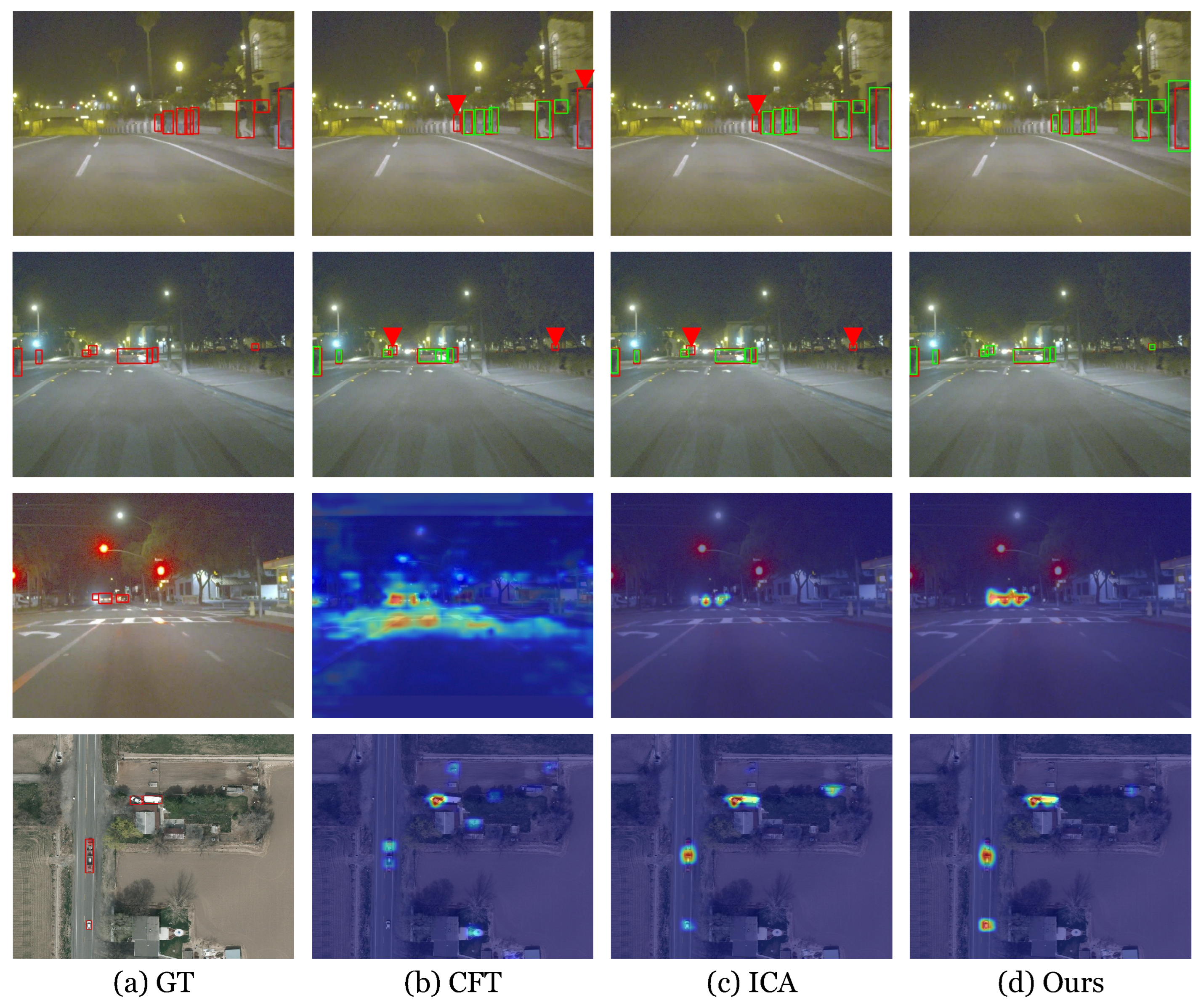
Heatmap visualization of various multimodal object detection methods on the LLVIP dataset. The first row shows the RGB images annotated with GroundTruth. The second and third rows depict the heatmap visualization results of the ICA and CFT methods, respectively. The last row presents our heatmap visualization results. Red bounding boxes indicate GroundTruth. The color intensity in the heatmaps reflects the response strength, where warmer colors (e.g., green/yellow) denote higher responses and cooler colors (e.g., blue) indicate lower responses.
Figure 10.
Heatmap visualization of various multimodal object detection methods on the LLVIP dataset. The first row shows the RGB images annotated with GroundTruth. The second and third rows depict the heatmap visualization results of the ICA and CFT methods, respectively. The last row presents our heatmap visualization results. Red bounding boxes indicate GroundTruth. The color intensity in the heatmaps reflects the response strength, where warmer colors (e.g., green/yellow) denote higher responses and cooler colors (e.g., blue) indicate lower responses.
Figure 11.
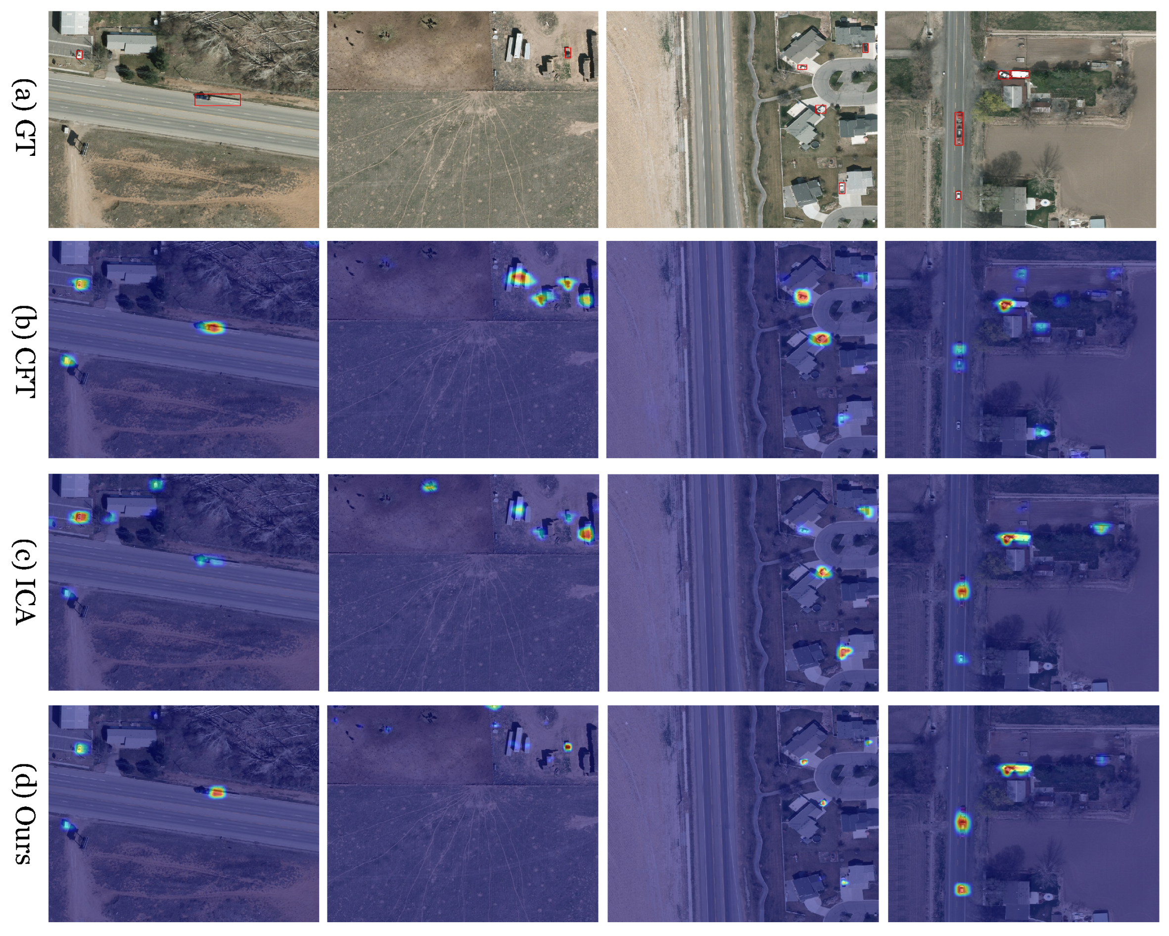
Heatmap visualization of various multimodal object detection methods on the VEDAI dataset. The first row shows the RGB images annotated with GroundTruth. The second and third rows depict the heatmap visualization results of the CFT and ICA methods, respectively. The last row presents our heatmap visualization results. Red bounding boxes indicate GroundTruth. The color intensity in the heatmaps reflects the response strength, where warmer colors (e.g., green/yellow) denote higher responses and cooler colors (e.g., blue) indicate lower responses.
Figure 11.
Heatmap visualization of various multimodal object detection methods on the VEDAI dataset. The first row shows the RGB images annotated with GroundTruth. The second and third rows depict the heatmap visualization results of the CFT and ICA methods, respectively. The last row presents our heatmap visualization results. Red bounding boxes indicate GroundTruth. The color intensity in the heatmaps reflects the response strength, where warmer colors (e.g., green/yellow) denote higher responses and cooler colors (e.g., blue) indicate lower responses.
Figure 12.
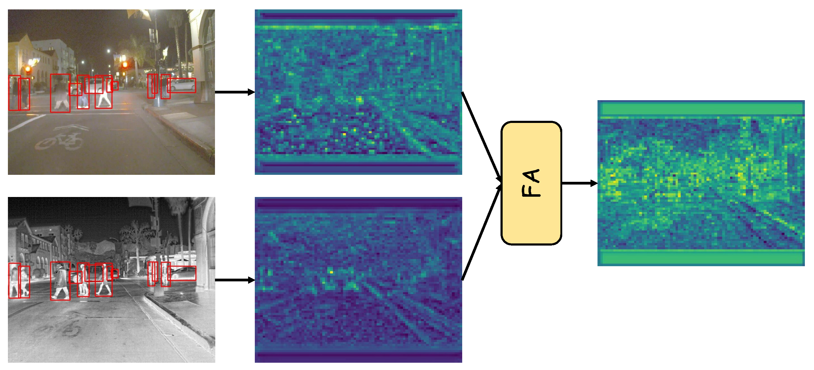
Visualization of module-specific feature evolution. From left to right: input RGB and infrared images, RGB and IR features before the Feature Aggregator (FA) module, and fused features after the FA module. Due to resizing to a uniform input size during training, some padding regions appear in the feature maps as areas with little or no activation. This illustrates how the FA module integrates cross-modal information and enhances semantic representations. Red bounding boxes indicate GroundTruth. The color intensity in the heatmaps reflects the response strength, where warmer colors (e.g., green/yellow) denote higher responses and cooler colors (e.g., blue) indicate lower responses.
Figure 12.
Visualization of module-specific feature evolution. From left to right: input RGB and infrared images, RGB and IR features before the Feature Aggregator (FA) module, and fused features after the FA module. Due to resizing to a uniform input size during training, some padding regions appear in the feature maps as areas with little or no activation. This illustrates how the FA module integrates cross-modal information and enhances semantic representations. Red bounding boxes indicate GroundTruth. The color intensity in the heatmaps reflects the response strength, where warmer colors (e.g., green/yellow) denote higher responses and cooler colors (e.g., blue) indicate lower responses.
Table 1.
Training hyperparameters for different datasets.
Table 1.
Training hyperparameters for different datasets.
| Dataset | lr0 | lrf | Momentum | Weight Decay |
|---|
| FLIR | 0.10 | 0.02 | 0.937 | 0.0005 |
| LLVIP | 0.05 | 0.10 | 0.937 | 0.0005 |
| VEDAI | 0.02 | 0.20 | 0.937 | 0.0005 |
Table 2.
Quantitative comparison with state-of-the-art methods on the FLIR dataset. The best results are highlighted in bold.
Table 2.
Quantitative comparison with state-of-the-art methods on the FLIR dataset. The best results are highlighted in bold.
| Methods | Backbone | Modality | mAP50 | mAP75 | mAP |
|---|
| YOLOv5-L [42] | YOLOv5 | RGB | 59.8 | 21.6 | 28.0 |
| YOLOv5-L [42] | YOLOv5 | IR | 74.8 | 35.3 | 39.6 |
| YOLOv8-L [48] | YOLOv8 | RGB | 63.6 | 25.0 | 30.4 |
| YOLOv8-L [48] | YOLOv8 | IR | 76.8 | 38.2 | 41.7 |
| (2021) CFT [39] | YOLOv5 | RGB + IR | 78.7 | 35.5 | 40.2 |
| (2023) CSAA [33] | ResNet50 | RGB + IR | 79.2 | 37.4 | 41.3 |
| (2023) ICAFusion [40] | YOLOv5 | RGB + IR | 79.2 | 36.9 | 41.4 |
| (2024) RSDet [34] | ResNet50 | RGB + IR | 81.1 | - | 41.4 |
| (2024) CrossFormer [38] | YOLOv5 | RGB + IR | 79.3 | - | 42.1 |
| Ours | Ours | RGB + IR | 80.4 | 38.8 | 42.8 |
Table 3.
Quantitative comparison with state-of-the-art methods on the LLVIP dataset. The best results are highlighted in bold.
Table 3.
Quantitative comparison with state-of-the-art methods on the LLVIP dataset. The best results are highlighted in bold.
| Methods | Modality | Backbone | mAP50 | mAP |
|---|
| YOLOv5-L [42] | RGB | YOLOv5 | 89.8 | 50.4 |
| YOLOv5-L [42] | IR | YOLOv5 | 95.7 | 61.9 |
| YOLOv8-L [48] | RGB | YOLOv8 | 91.9 | 54.0 |
| YOLOv8-L [48] | IR | YOLOv8 | 95.2 | 62.1 |
| (2019) Cascade R-CNN [49] | RGB | ResNet50 | 88.3 | 47.0 |
| (2019) Cascade R-CNN [49] | IR | ResNet50 | 95.0 | 56.8 |
| (2023) DIVFusion [19] | RGB + IR | YOLOv5 | 89.8 | 52.0 |
| (2023) CSAA [33] | RGB + IR | ResNet50 | 94.3 | 59.2 |
| (2024) RSDet [34] | RGB + IR | ResNet50 | 95.8 | 61.3 |
| (2021) CFT [39] | RGB + IR | YOLOv5 | 97.5 | 63.6 |
| (2024) ICAFusion [40] | RGB + IR | YOLOv5 | 97.5 | 63.7 |
| (2025) FQDNet [50] | RGB + IR | YOLOv8 | 96.4 | 64.1 |
| (2025) EI2Det [51] | RGB + IR | YOLOv8 | 98.0 | 63.9 |
| (2025) FusionMamba [52] | RGB + IR | YOLOv8 | 97.0 | 64.3 |
| Ours | RGB + IR | Ours | 97.7 | 66.6 |
Table 4.
Quantitative comparison with state-of-the-art methods on the VEDAI dataset. The best results are highlighted in bold.
Table 4.
Quantitative comparison with state-of-the-art methods on the VEDAI dataset. The best results are highlighted in bold.
| Methods | Backbone | Modality | mAP50 | mAP75 | mAP |
|---|
| YOLOv5-L [42] | YOLOv5 | RGB | 57.3 | 30.6 | 32.4 |
| YOLOv5-L [42] | YOLOv5 | IR | 58.4 | 32.9 | 33.2 |
| (2021) CFT [39] | YOLOv5 | RGB + IR | 67.8 | 43.3 | 39.6 |
| (2024) ICAFusion [40] | YOLOv5 | RGB + IR | 73.5 | 42.6 | 42.0 |
| (2025) EI2Det [51] | YOLOv8 | RGB + IR | 75.6 | 43.8 | 44.0 |
| Ours | Ours | RGB + IR | 74.7 | 53.0 | 45.5 |
Table 5.
Inference time and FPS comparison of different methods on the VEDAI dataset.
Table 5.
Inference time and FPS comparison of different methods on the VEDAI dataset.
| Methods | Time (ms) | FPS |
|---|
| YOLOv5-L [42] | 8.8 | 113.6 |
| (2024) ICAFusion [40] | 13.9 | 71.9 |
| (2021) CFT [39] | 15.6 | 64.1 |
| (2025) FusionMamba [52] | 89.9 | 11.1 |
| Ours | 77.9 | 12.8 |
Table 6.
Ablation study of FE and FA modules on the VEDAI dataset. The best results are highlighted in bold.
Table 6.
Ablation study of FE and FA modules on the VEDAI dataset. The best results are highlighted in bold.
| Model | mAP50 | mAP75 | mAP | Params |
|---|
| Baseline | 68.8 | 40.5 | 39.8 | 51.7 M |
| Baseline + FE | 66.8 | 46.2 | 42.0 | 145.2 M |
| Baseline + FE + FA | 74.7 | 53.0 | 45.5 | 277.1 M |
Table 7.
Ablation study of FE and FF modules on the FLIR dataset. The best results are highlighted in bold.
Table 7.
Ablation study of FE and FF modules on the FLIR dataset. The best results are highlighted in bold.
| Model | mAP50 | mAP75 | mAP | Params |
|---|
| Baseline | 79.6 | 37.0 | 41.3 | 51.7 M |
| Baseline + FE | 79.4 | 38.8 | 42.0 | 145.2 M |
| Baseline + FE + FA | 80.4 | 38.8 | 42.8 | 277.1 M |
Table 8.
Ablation study results on the number of FA modules. The best results are highlighted in bold.
Table 8.
Ablation study results on the number of FA modules. The best results are highlighted in bold.
| Number | mAP50 | mAP75 | mAP | Params |
|---|
| 1 | 81.1 | 36.6 | 41.8 | 178.3 M |
| 2 | 78.8 | 36.6 | 41.1 | 211.4 M |
| 3 | 79.0 | 37.3 | 41.4 | 244.5 M |
| 4 | 80.4 | 38.8 | 42.8 | 277.1 M |
Table 9.
Ablation study of the proposed Patch-based Feature Enhancer (PFE) and Patch-based Feature Aggregator (PFA) on the VEDAI dataset. The best results are highlighted in bold.
Table 9.
Ablation study of the proposed Patch-based Feature Enhancer (PFE) and Patch-based Feature Aggregator (PFA) on the VEDAI dataset. The best results are highlighted in bold.
| Model | mAP50 | mAP75 | mAP |
|---|
| Ours | 74.7 | 53.0 | 45.5 |
| w/o PFE | 74.5 | 50.4 | 44.2 |
| w/o PFA | 69.0 | 47.4 | 42.3 |