Evaluation of Seismo-Ionospheric and Seismological Parameters Within the Lithosphere–Atmosphere–Ionosphere Coupling Framework for the 2025 Mw 7.7 Myanmar Earthquake

Highlights

What are the main findings?

• Multi-parameter GNSS-TEC and b-value mapping reveal seismo-ionospheric coupling.
• Negative TEC anomaly (~30 TECU below threshold) was detected three days before the earthquake under geomagnetically quiet conditions.

What are the implications of the main findings?

• b-value drop (1.12 → 0.58) and high RSHI overlap indicate progressive stress accumulation.
• KDE shows a low-b, low-vTEC cluster, supporting stress–ionosphere coupling during the preparation phase.

Abstract

This study presents a comprehensive multi-parameter analysis of seismo-ionospheric responses to the Mw 7.7 Myanmar earthquake on 28 March 2025, using GNSS-based Total Electron Content (TEC) data, seismic b-value trends, and acoustic gravity wave (AGW) signatures. A significant negative TEC anomaly (~30 TECU below the statistical threshold) was detected on 25 March, three days before the mainshock under geomagnetically quiet conditions, indicating a lithospheric origin. Concurrent variations in the Ionospheric Disturbance Index (IDI) and Rate of TEC Index (ROTI) indicate pronounced background departures and enhanced short-term variability during the preparation phase. Temporal b-value analysis shows a consistent decline from 1.12 to 0.58 across the 30-year to 6-month windows, with the lowest values clustering near the epicenter, indicating progressive stress accumulation. Spatial b-value mapping further reveals a low b-value zone overlapping the region of TEC depletion, while the Relative Seismic Hazard Index (RSHI) highlights high-hazard zones aligned with the epicentral area. Kernel density estimation (KDE) supports this coupling by showing a dominant low-b, low-vTEC cluster, consistent with linked lithospheric stress and ionospheric depletion. Overall, the integrated GNSS and seismic analyses demonstrate the value of multi-domain observations for characterizing earthquake preparation processes, highlighting a coherent physical linkage between crustal stress accumulation and ionospheric depletion that can enhance short-term seismic hazard assessment.

1. Introduction

Earth’s lithosphere and ionosphere are closely linked by a complex cascade of physical processes, most importantly in the presence of seismic instability. Over the past few decades, advancements in space geodetic technologies, particularly Global Navigation Satellite Systems (GNSS), have enabled the hitherto impossible capacity to monitor ionospheric disturbances in near real time. Of prime interest is the Total Electron Content (TEC), a significant ionospheric parameter dynamically sensitive to space weather conditions and lithospheric activity, i.e., earthquakes. TEC represents the total number of electrons present along a one-meter-square column between a GNSS satellite and a ground-based receiver and is commonly used to quantify ionospheric charge density variations [1,2]. The two-way sensitivity of TEC renders it an excellent precursory signal in seismo-ionospheric coupling studies. On the other hand, statistically, by way of the b-value, derived from the Gutenberg–Richter law [3], and further refined by Aki’s maximum likelihood method [4], seismological characteristics such as b-value are an important criterion to determine the condition of crustal stress and earthquake potential. The b-value characterizes the relative proportion of small to large earthquakes in a region; a low b-value typically signifies high tectonic stress and potential rupture zones, while a higher b-value reflects a more stable or less stressed crust [5,6]. Although, TEC anomalies and b-value variations have been independently investigated as earthquake-related indicators, a quantitative framework capable of jointly assessing their spatial and statistical correspondence remains largely unexplored. This gap limits the ability to distinguish physically meaningful precursors from coincidental overlaps.

The first efforts to study the ionospheric response to seismic activity date to the late 1960s, during which unusual propagations of radio waves were recorded before major earthquakes. Only with the advent of GNSS during the 1990s did systematic studies of earthquake precursors based on TEC begin to gain momentum. Liu et al. [7,8] provided some of the earliest statistical evidence linking TEC disruptions with pre-earthquake states throughout Taiwan, finding reproducible anomalies that occurred prior to large events days ahead of time. Later case studies have come to further endorse the presence of ionospheric disturbances prior to great earthquakes [9,10,11,12,13,14,15,16]. These studies demonstrated that pre-seismic TEC anomalies will manifest in an explicitly well-defined spatial radius, typically estimated through Dobrovolsky’s empirical relation [17], and as positive or negative perturbations. This recent renewal of attention to the results spurred the development of other indexes to quantify the anomalies, such as the Ionospheric Disturbance Index (IDI) [18] and the Rate of TEC Index (ROTI) [19], which help to separate seismo-ionospheric signals from background noise.

Concurrently, seismic b-value has evolved as the most reliable statistical indicator of the likelihood of earthquake occurrence. According to Gutenberg–Richter law, the b-value quantifies the relative frequency of small and great earthquakes and is inversely related to the stress regime of the lithosphere. Numerous studies have shown that spatial and temporal variations in b-values are very useful for forecasting future seismicity [20,21,22]. In particular, decreasing b-value is routinely observed in regions of increasing tectonic stress and has been noted as a typical precursor to great earthquakes. Application of b-value mapping to seismic hazard analysis has been global, transgressing tectonic boundaries as well as intraplate regions [23,24,25].

Despite these concurrent advances, there are still some gaps in the integration of ionospheric and seismic hazard proxies. TEC and b-value each provide indicative indicators autonomously from earthquake-related processes, but interactions between ionospheric anomalies and seismogenic stress conditions have been relatively understudied. A few investigations [14,26] proposed the possibility that the spatial distribution of ionospheric TEC anomalies could coincide with high-stress areas delineated by low b-value regions. However, no quantitative approach to investigating the correlation in time and space is currently available. The theoretical background for merging TEC anomalies and b-value distributions is the lithosphere–atmosphere–ionosphere coupling (LAIC) model. This model suggests that tectonic stress accumulation before an earthquake could cause the release of radon and other gases, which in turn modify the atmospheric electric field and cause vertical plasma drift in the ionosphere, leading to TEC perturbations that are detectable [27,28]. At the same time, the same regions with increased stress are statistically defined by a low b-value signature. Thus, these two physically connected but contrasting observables, ionospheric anomalies and b-values, may be conveying the same preparatory process but in different domains. Their spatial congruence can be utilized to possibly uncover seismically responsive ionospheric areas and increase the confidence of earthquake precursors.

The catastrophic Mw 7.7 Myanmar earthquake that happened on 28 March 2025 provides an interesting case study to investigate this integrated method. Located in a general complicated tectonic setting brought about by the collision between the Indian and Eurasian plates, Myanmar is an actively seismic area that has experienced several significant earthquakes over the past hundred years [29]. However, with some exceptions, pre-seismic monitoring and seismic hazard evaluation efforts in this area are primarily grounded on seismically recorded data from the ground surface, with minimal utilization of atmospheric or ionospheric datasets. The 2025 Myanmar event, due to its high magnitude, shallow depth, and significant ionospheric footprint, offers a unique case for evaluating the potential of TEC–b-value coupling in pre-seismic monitoring. This study is motivated by two key considerations. First, previous research suggests that pre-seismic TEC perturbations, quantifiable through IDI and ROTI parameters, may occur several days before major earthquakes [30]. Second, b-value mapping of historical seismicity in tectonically active regions is hypothesized to reveal zones of low b-values that align with stress accumulation zones and known fault segments [31]. By combining these two perspectives, we aim to establish a methodological bridge between ionospheric monitoring and seismic hazard assessment. The central hypothesis is that regions showing strong pre-seismic TEC anomalies tend to align with zones of low b-values and higher relative seismic hazard, reflecting a coupled lithosphere–ionosphere system. The importance of this study lies in its potential to enhance short-term earthquake forecasting through multi-domain integration. By validating the spatial and temporal association between TEC anomalies and b-values, we can refine earthquake preparation zone identification, support early-warning system development, and reduce false positives caused by geomagnetic or space weather activity. Moreover, by applying this framework to a real case, the 28 March 2025 Myanmar earthquake, this research offers tangible insights into how GNSS-based ionospheric monitoring can complement seismic hazard metrics in a high-risk, data-sparse region.

Accordingly, the objectives of this study are fourfold: (1) to extract and characterize ionospheric TEC anomalies before the 28 March 2025 Myanmar earthquake using GNSS data; (2) to compute IDI and ROTI to quantify ionospheric perturbations and identify significant pre-seismic disturbances; (3) to analyze the spatial distribution of b-values and derive a relative seismic hazard map based on long-term earthquake catalogs; and (4) to correlate the spatial overlap between strong TEC anomalies and low b-value zones, thereby validating the theoretical coupling between the ionosphere and lithospheric stress. Through this integrated approach, this study aims to advance the frontier of seismo-ionospheric research by demonstrating the added value of TEC–b-value synergy in seismic hazard characterization. By drawing upon both atmospheric and solid Earth datasets, this work promotes a more comprehensive, cross-domain understanding of earthquake preparation processes and opens new pathways for multi-parametric earthquake monitoring in tectonically vulnerable regions.

2. Materials and Methods

2.1. Data Acquisition

Understanding the lithosphere–ionosphere coupling processes that precede large earthquakes requires the careful integration of multi-domain geophysical datasets. In this study, we assembled a diverse suite of data spanning ionospheric, geomagnetic, and seismic observations to investigate precursory signatures associated with the Mw 7.7 Myanmar earthquake that occurred near Mandalay, Myanmar, on 28 March 2025 at 06:20:52 (UTC), with an epicenter located at 22.001°N, 95.925°E and a focal depth of 15.0 km (USGS). Each dataset was selected not only for its scientific relevance but also for its spatial and temporal resolution to capture subtle signals preceding the mainshock.

2.1.1. Ionospheric TEC Data

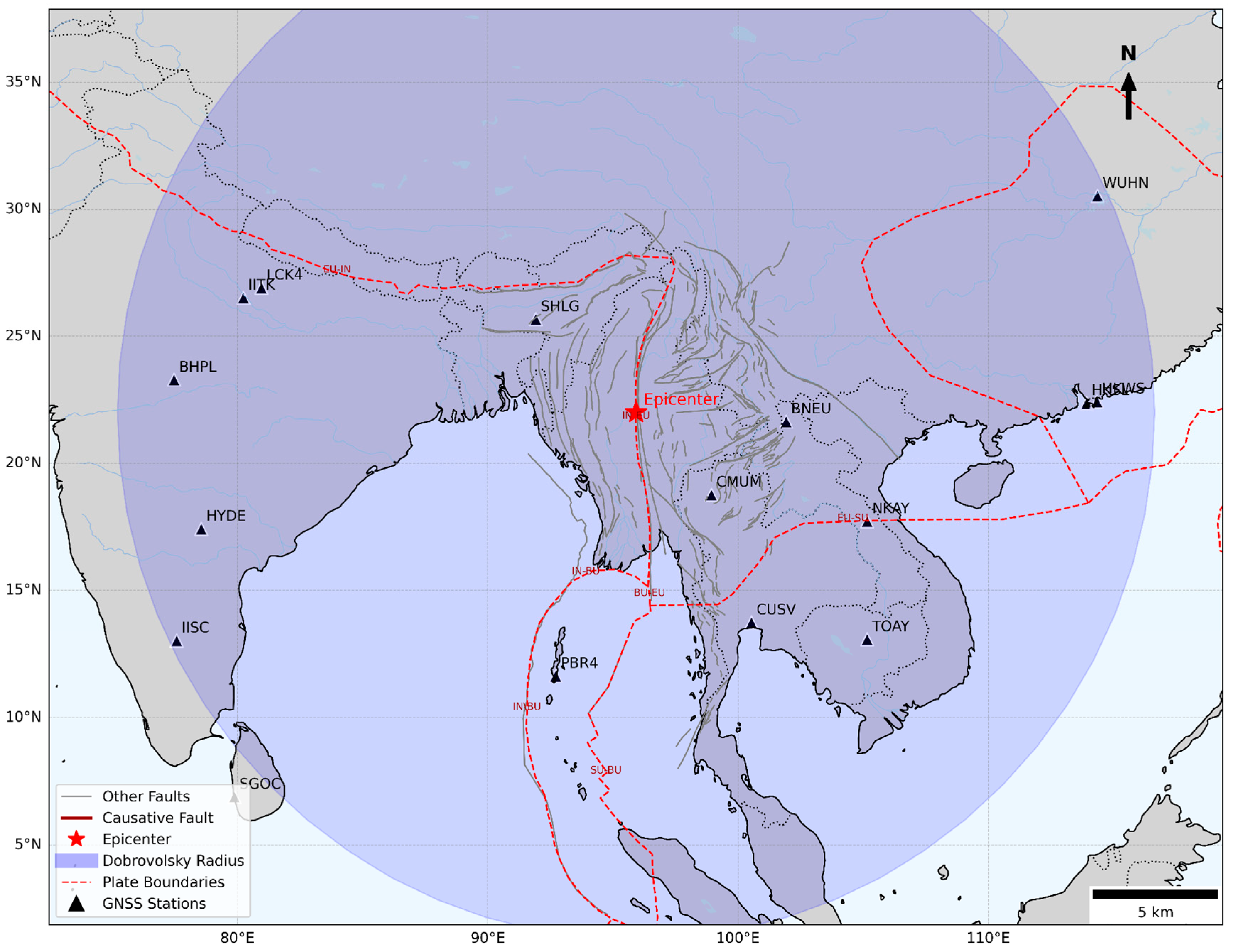
To investigate the ionospheric precursors associated with the Myanmar earthquake, GNSS-based TEC data were analyzed from a network of 16 strategically located GNSS stations surrounding the earthquake epicenter, covering a wide regional footprint across Myanmar and adjacent areas. The spatial configuration of these stations allowed for high-resolution spatial–temporal assessment of ionospheric variations potentially linked to pre-seismic lithospheric activity. Continuous GNSS observations from these stations were acquired for the period 15 February to 31 March 2025, encompassing a 30-day window leading up to and including the day of the earthquake. The data were recorded at a high temporal resolution (1 min intervals), enabling the identification of both gradual and abrupt ionospheric anomalies over time. A complete summary of the GNSS stations, including their station codes, geographic coordinates (latitude and longitude), and epicentral distances, is provided in

Table 1. List of GNSS stations used in this study, including their locations and distances from the epicenter.

Station	Lat (°N)	Long (°E)	Dist. (km)	Station	Lat (°N)	Long (°E)	Dist. (km)
BHPL	23.289	77.467	1898.03	IITK	26.521	80.232	1666.65
BNEU	21.644	101.917	620.08	LCK4	26.912	80.956	1608.84
CMUM	18.761	98.932	477.69	NKAY	17.719	105.153	1076.04
CUSV	13.736	100.534	1040.33	PBR4	11.637	92.712	1201.84
HKSL	22.372	113.928	1853.29	SGOC	6.892	79.874	2205.54
HKWS	22.434	114.335	1894.85	SHLG	25.674	91.913	577.03
HYDE	17.417	78.551	1887.08	TOAY	13.073	105.153	1393.11
IISC	13.021	77.57	1984.32	WUHN	30.532	114.357	1964.54

. Their distribution is also visualized in Figure 1, which displays all stations relative to the earthquake epicenter and the Dobrovolsky radius.

2.1.2. Seismicity Data

To investigate the lithospheric conditions preceding the 2025 Myanmar earthquake, earthquake data from the United States Geological Survey (USGS) catalog were retrieved. The focus was on regional seismicity spanning the active tectonic corridor along the Sagaing Fault system and its surrounding zones. Only earthquakes with magnitudes ≥ 2.5 and focal depths ≤ 100 km were retained. The magnitude threshold corresponds to the estimated magnitude of completeness (Mc ≈ 2.5), ensuring data reliability, while the depth constraint focuses on crustal events capable of generating surface-coupled processes that can influence the atmosphere and ionosphere within the LAIC framework.

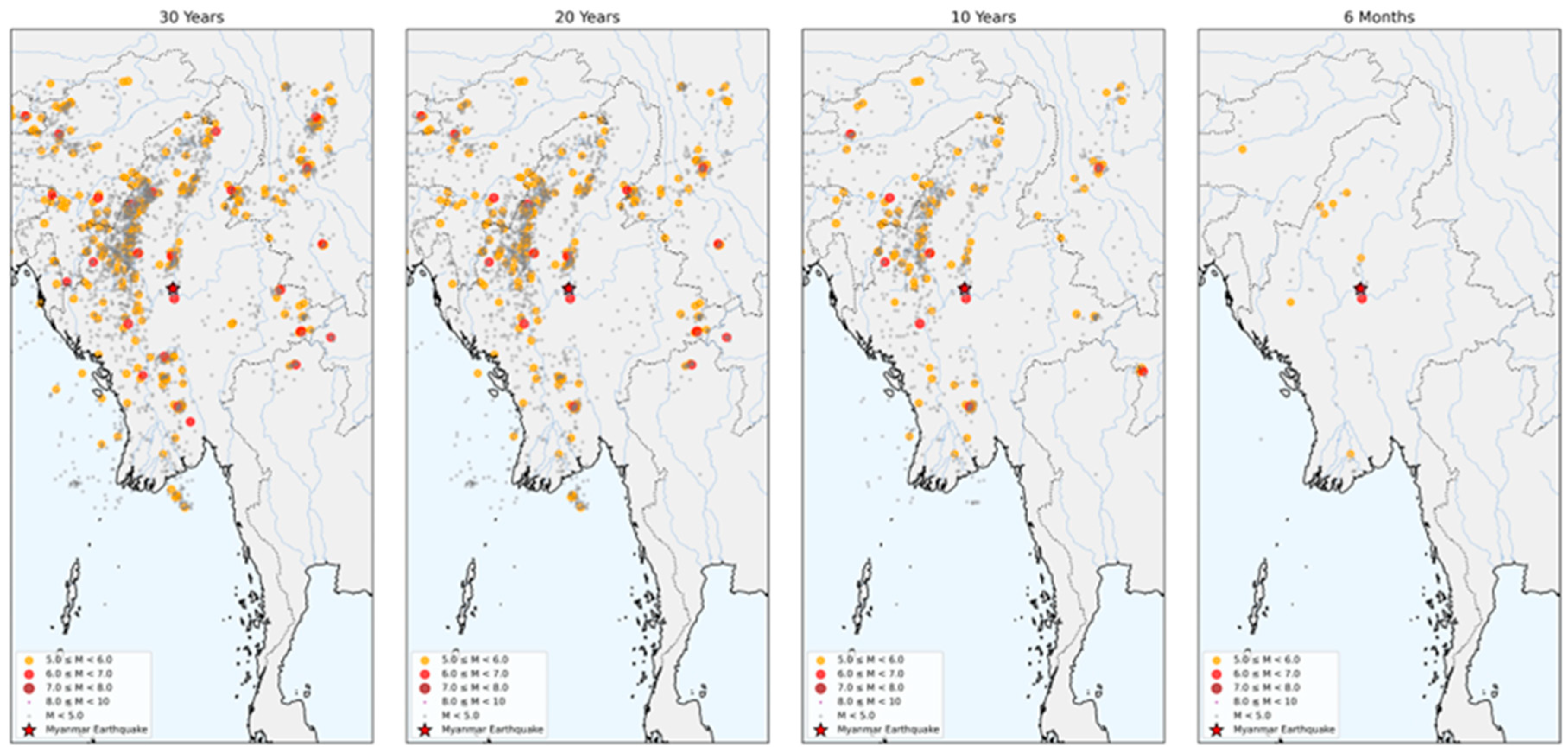
To capture the evolving state of seismicity over multiple timescales, four distinct seismic catalogs were constructed covering (i) the past 30 years (1995–2025), (ii) 20 years (2005–2025), (iii) 10 years (2015–2025), and (iv) the last 6 months leading up to the earthquake (28 March 2025). The rationale behind this multi-window approach lies in its ability to offer complementary temporal insights while the 30-year catalog establishes the long-term seismotectonic baseline; the shorter windows reveal progressive stress localization and foreshock activity, if any. The 6-month catalog, in particular, is essential for resolving potential immediate precursors in seismic behavior. Each catalog was subjected to a declustering process using the Gardner and Knopoff algorithm [32] to eliminate dependent events such as aftershocks and swarm sequences. This ensured the statistical independence of events used for further analysis. To visualize the spatial distribution of seismicity across all four catalogs, a composite map displaying the epicentral locations of earthquakes was generated within the defined region and timeframes, as shown in Figure 2.

2.2. TEC Calculation and Anomaly Detection Criteria

The RINEX observation files acquired from the 16 GNSS stations were processed to extract ionospheric TEC, enabling the identification of ionospheric anomalies preceding the 28 March 2025 Myanmar earthquake. These observations, originally recorded as dual-frequency carrier phase and pseudorange measurements, were essential for capturing the ionospheric state at minute-level temporal resolution [33]. Data processing was carried out using the GPS-TEC software Ver 3.5 developed by Gopi Seemala, which facilitates the derivation of sTEC from the L1 and L2 signal pairs [34,35], applying the standard formula as given in Equation (1):

$$sTEC={\displaystyle \frac{f_1^2\times f_2^2}{40.3\left(f_1^2-f_2^2\right)}} \left[\left(P_2-P_1\right)-\left(b_s-b_r\right)\right]$$

(1)

where sTEC is the slant TEC, f₁ and f₂ are the carrier frequencies, P₁ and P₂ are the pseudo ranges corresponding to the carrier frequencies, b_s is the satellite bias, and br is the receiver bias. To reduce the influence of satellite elevation angles on signal path lengths, the computed slant TEC was then converted into vertical TEC (vTEC) using a mapping function under the assumption of a thin-shell ionosphere fixed at 350 km altitude [33,36,37], as given in Equation (2):

$$vTEC=sTEC\times cos\left(arcsin\left({\displaystyle \frac{R_E\times cos\left(E\right)}{R_E+h}}\right)\right)$$

(2)

where R_E represents Earth’s radius (6371 km), E is the satellite elevation angle, and ℎ is the ionospheric shell height (350 km). The software implementation included built-in filters to exclude low-elevation satellite arcs (<15°) and to smooth short-term fluctuations likely caused by multipath or receiver noise.

Once vTEC time series were computed, the next objective was to identify potential ionospheric disturbances that could be interpreted as precursors to the earthquake. To this end, we applied a statistically grounded anomaly detection approach based on prior studies [13,16,38]. For every epoch across the observation window, 15-day rolling background mean (μ) and standard deviation (σ) were computed. These parameters formed the basis for constructing a dynamic anomaly envelope defined by Equation (3):

$$\mu \left(t\right)\pm 1.34\sigma \left(t\right)$$

(3)

This ±1.34σ threshold corresponds to a ~91% confidence level, offering a balanced trade-off between sensitivity and noise rejection, as stricter thresholds may suppress moderate but physically meaningful pre-seismic anomalies. Any TEC value breaching this envelope was flagged as an anomaly. Specifically, data points exceeding the upper bound (μ + 1.34σ) were classified as positive anomalies, while those falling below the lower bound (μ − 1.34σ) were categorized as negative anomalies. To quantify the extent of these perturbations, peak anomalies were calculated by identifying the highest and lowest departures from the rolling mean, as given by Equations (4) and (5):

$$Peak Positive Anomaly=max\left[vTEC\left(t\right)-\mu \left(t\right)\right] \mathrm{f}\mathrm{o}\mathrm{r} vTEC\left(t\right)>\mu \left(t\right)+1.34\sigma$$

(4)

$$Peak Negative Anomaly=min\left[vTEC\left(t\right)-\mu \left(t\right)\right] \mathrm{f}\mathrm{o}\mathrm{r} vTEC\left(t\right)<\mu \left(t\right)-1.34\sigma$$

(5)

To ensure that identified anomalies were not influenced by external space weather conditions, the methodology explicitly excluded days with elevated geomagnetic activity, defined by thresholds of Dst < −30 nT, Kp > 3, or Ap > 20 [39,40]. This geomagnetic filtering step was systematically applied to isolate seismogenic ionospheric perturbations and improve the reliability of anomaly detection linked to tectonic stress buildup.

2.3. Ionospheric Disturbance Index (IDI) and Rate of TEC Index (ROTI) Calculation

In addition to the statistical anomaly detection of TEC described previously, we applied two well-established ionospheric perturbation indices, IDI and ROTI, to further characterize both large-scale anomalies and small-scale irregularities during the earthquake preparation period.

The IDI serves as a station-wise metric for capturing the overall intensity of TEC deviations from its climatological behavior. It is particularly useful for summarizing cumulative TEC perturbations within a given day or time window. For each station, the IDI was computed by comparing the absolute TEC deviations against the rolling statistical baseline (mean and standard deviation) derived as in Section 2.2. The formula used is given in Equation (6):

$${IDI}_i={\displaystyle \frac{1}{N}}\sum _{j=i}^N\left({\displaystyle \frac{\left|{vTEC}_{i,j}-{\mu }_j\right|}{{\sigma }_j}}\right)$$

(6)

where ${vTEC}_{i,j}$ is the vertical TEC value at tile epoch j for station i, and ${\mu }_j$ and ${\sigma }_j$ represent the mean and standard deviation for that epoch calculated from the background period. The index is normalized across all epochs N, providing a daily disturbance score for each GNSS station. Higher IDI values indicate stronger strength of ionospheric deviations from background behavior.

In parallel, we computed the ROTI, which quantifies short-term ionospheric fluctuations associated with small-scale plasma irregularities. This index is especially sensitive to rapid, transient changes in TEC, which are often indicative of equatorial spread F, traveling ionospheric disturbances (TIDs), or earthquake-coupled electric field responses. ROTI is defined as the standard deviation of the Rate of TEC (ROT) over a sliding time window [41,42] and is given by Equations (7) and (8):

$${ROT}_i\left(t\right)={\displaystyle \frac{{vTEC}_i\left(t+∆t\right)-{vTEC}_i\left(t\right)}{∆t}}$$

(7)

$${ROTI}_i\left(t\right)=\sqrt{〈{\left({ROT}_i\left(t\right)-〈{ROT}_i\left(t\right)〉\right)}^2〉}$$

(8)

where ∆t corresponds to a 1 min sampling interval and $〈{ROT}_i\left(t\right)〉$ denotes averaging over a 5 min window. The resulting ROTI values reflect the standard deviation of TEC rate changes within that short window, revealing bursty irregularities that are otherwise undetected by statistical anomaly methods or IDI.

2.4. Acoustic Gravity Wave (AGW) Detection via Wavelet Analysis

To explore the presence of transient atmospheric disturbances preceding the 28 March 2025 Myanmar earthquake, ionospheric TEC oscillations associated with AGWs were investigated. AGWs are vertically propagating disturbances that originate from impulsive processes near the Earth’s surface such as fault rupture or ground shaking and transmit energy upward through the neutral atmosphere into the ionosphere [43,44,45]. When they reach F-region altitudes (~300–400 km), these waves induce oscillatory perturbations in electron density, which are reflected as periodic structures in TEC time series [46]. For this analysis, a wavelet-based spectral technique that isolates transient oscillatory waveforms in the time–frequency domain was employed. This approach is particularly well-suited for non-stationary geophysical signals and has been widely adopted in AGW detection studies [47,48]. The raw vTEC series, computed at 1 min intervals, was first detrended using a 60 min moving average to remove slow background variations. The residual component containing high-frequency ionospheric fluctuations was then subjected to Continuous Wavelet Transform (CWT) using the Morlet wavelet as the mother function [49]. The Morlet wavelet offers optimal resolution in both the time and frequency domains and is particularly effective for identifying quasi-harmonic features such as AGWs.

Mathematically, the CWT is defined as given in Equation (9) [47,50]:

$$W\left(s,\tau \right)={\displaystyle \frac{1}{\sqrt{\left|s\right|}}}{\int }_{-\propto }^{\propto }\int TEC\left(t\right){\psi }^{*}\left({\displaystyle \frac{t-\tau }{s}}\right)dt$$

(9)

where W(s,τ) represents the wavelet coefficients, s is the scale parameter corresponding inversely to frequency (i.e., larger s captures lower-frequency waves), τ is the transition parameter, ${\psi }^{*}$ is the complex conjugate of the Morlet wavelet function, and TEC(t) is the detrended TEC time series.

The square magnitude of the wavelet coefficients, ${\left|W\left(s,\tau \right)\right|}^2$, represents the wavelet power spectrum, which reveals how oscillation energy is distributed over time and across frequency bands. Power-Frequency Distribution (PFD) graphs were generated for every station showing dominant periodic components of AGW signatures. To quantify AGW strength, the total wavelet power within the AGW-sensitive frequency band for each day was extracted, averaged across time using Equation (10):

$${AGW}_{power}\left(d\right)={\displaystyle \frac{1}{T}}\sum _{t=1}^T{\int }_{f_1}^{f_2}{\left|W\left(f,t\right)\right|}^{2}df$$

(10)

where ${AGW}_{power}\left(d\right)$ denotes the daily averaged AGW power, T is the total number of time steps in the day, and f1 and f2 represent the lower and upper limits of the AGW-relevant frequency range.

2.5. Spatial Interpolation of TEC

To analyze the spatial characteristics of ionospheric perturbations, we performed spatial interpolation of vTEC using the Ordinary Kriging method. This geostatistical approach is well-suited for reconstructing spatially continuous TEC fields from irregularly distributed GNSS stations, enabling the visualization of ionospheric morphology during quiet and anomalous conditions. The rationale for using Kriging stems from its ability to incorporate both spatial autocorrelation and localized station measurements into an optimal interpolation framework [51,52]. Unlike simple deterministic methods such as inverse distance weighting, Kriging generates statistically unbiased estimates with minimized error variance, making it ideal for ionospheric mapping with sparse-to-moderate GNSS coverage. The Ordinary Kriging estimator used in this study is defined as Equation (11):

$$Z\left(x_0\right)= \sum _{i=1}^n{\lambda }_{i}Z\left(x_i\right)$$

(11)

where $Z\left(x_i\right)$ are observed values and ${\lambda }_i$ are weights derived from a fitted spherical semivariogram model. Kriging provides best linear unbiased estimates, making it suitable for resolving subtle TEC gradients across sparse station networks.

2.6. b-Value Estimation and Seismic Hazard Mapping

To characterize crustal stress heterogeneity and estimate the relative seismic hazard potential of the Myanmar region, we first computed the b-value across a spatial grid using a 30-year earthquake catalog (1995–2025). Events with magnitudes ≥ 2.5 and depths ≤ 100 km were retained and declustered to ensure statistical independence. The region was divided into 0.2° × 0.2° grid cells, and b-values were calculated for each cell containing at least 10 events, using the maximum likelihood method proposed by [4]:

$$b= {\displaystyle \frac{{log}_{10}e}{\overline{M}-M_c}}$$

(12)

where $\overline{M}$ is the average magnitude of events in the cell and $M_c$ is the local magnitude of completeness, estimated from the peak of the magnitude histogram.

To integrate these seismicity metrics into a coherent spatial hazard framework, we developed a Relative Seismic Hazard Index (RSHI). This index synthesizes both the b-value and the local seismicity rate (event density) into a dimensionless hazard index. First, the b-values were inverted and normalized to emphasize low-b (high-stress) zones, while event densities were min–max normalized, given by Equations (13) and (14):

$$b^{*}={\displaystyle \frac{1.5-b}{1.0}}$$

(13)

$${\rho }^{*}={\displaystyle \frac{\rho -{\rho }_{min}}{{\rho }_{max}-{\rho }_{min}}}$$

(14)

where $b^{*}$ and ${\rho }^{*}$ are the normalized b-value and event density, respectively. The final hazard score H was computed as the weighted average given by Equation (15):

$$H= 0.5·b^{*}+0.5·{\rho }^{*}$$

(15)

This formulation ensures equal contribution from both stress indicators and occurrence frequency. The hazard scores were then spatially interpolated using Ordinary Kriging, employing a spherical variogram model to generate a continuous hazard field over the region. The resulting Relative Seismic Hazard Map delineates areas of high and low seismic potential. Hazard scores range from 0 (low hazard) to 1 (high hazard). This mapping framework not only highlights seismically active zones but also enables correlation with ionospheric anomaly locations, offering a powerful tool for integrating lithospheric stress and ionospheric response into a unified earthquake precursor framework.

2.7. Correlation Analysis Using Kernel Density Estimation

To quantitatively assess the coupling between lithospheric stress and ionospheric anomalies, we conducted a joint statistical analysis of seismic b-values and interpolated vTEC using kernel density estimation (KDE) [53] and quadrant-based classification [54]. This allowed us to explore whether regions of high ionospheric perturbation coincide with low b-value zones, thereby supporting the hypothesis of pre-earthquake lithosphere–ionosphere interaction. The analysis was performed on a merged dataset containing spatially matched b-values and interpolated vTEC values. KDE was selected for its ability to generate a smooth, continuous approximation of the joint probability distribution P(b,vTEC) without assuming any underlying distributional form [55,56]. The bivariate kernel density estimate (Equation (16)) was computed following the seminal works by Silverman [57] and Scott [58]:

$$\widehat{f}(b,v)= {\displaystyle \frac{1}{n{h}_b{h}_v}}\sum _{i=1}^{n}K\left({\displaystyle \frac{b-b_i}{h_b}}\right)K\left({\displaystyle \frac{v-v_i}{v_b}}\right)$$

(16)

where $\widehat{f}(b,v)$ is the joint KDE over b-value and vTEC, $n$ is the number of observations, $h_b$ and $h_v$ are the bandwidths for b and vTEC, and $K\left(·\right)$ is the Gaussian kernel function.

To further formalize this relationship, we applied a quadrant-based classification scheme, dividing the joint b–TEC anomaly space into four domains using the median values of b-value (b_0.5) and vTEC anomaly (ΔTEC_0.5), as provided in Equation (17):

$$Quadrant \left(i\right)=\left\{\begin{array}{c}\begin{array}{c}Q1 if b_i\le b_{0.5} \wedge {\mathsf{\Delta }TEC}_i\le {\mathsf{\Delta }TEC}_{0.5}\\ Q2 if b_i>b_{0.5} \wedge {\mathsf{\Delta }TEC}_i\le {\mathsf{\Delta }TEC}_{0.5}\\ Q3 if b_i\le b_{0.5} \wedge {\mathsf{\Delta }TEC}_i>{\mathsf{\Delta }TEC}_{0.5}\end{array}\\ Q4 if b_i>b_{0.5} \wedge {\mathsf{\Delta }TEC}_i>{\mathsf{\Delta }TEC}_{0.5}\end{array}\right\}$$

(17)

Each spatial point was assigned to one of the four quadrants, and the frequency of points in each class was computed. Particular focus was placed on quadrant Q1 (low-b, negative ΔTEC), which is hypothesized to represent zones of enhanced lithospheric stress accumulation associated with pre-seismic ionospheric depletion. An overrepresentation of this quadrant would indicate a statistically significant association between mechanically unstable crustal regions and anomalous ionospheric depletion, providing quantitative support for seismo-ionospheric coupling during the earthquake preparation phase.

3. Results and Analysis

3.1. Temporal Evolution of TEC Anomalies

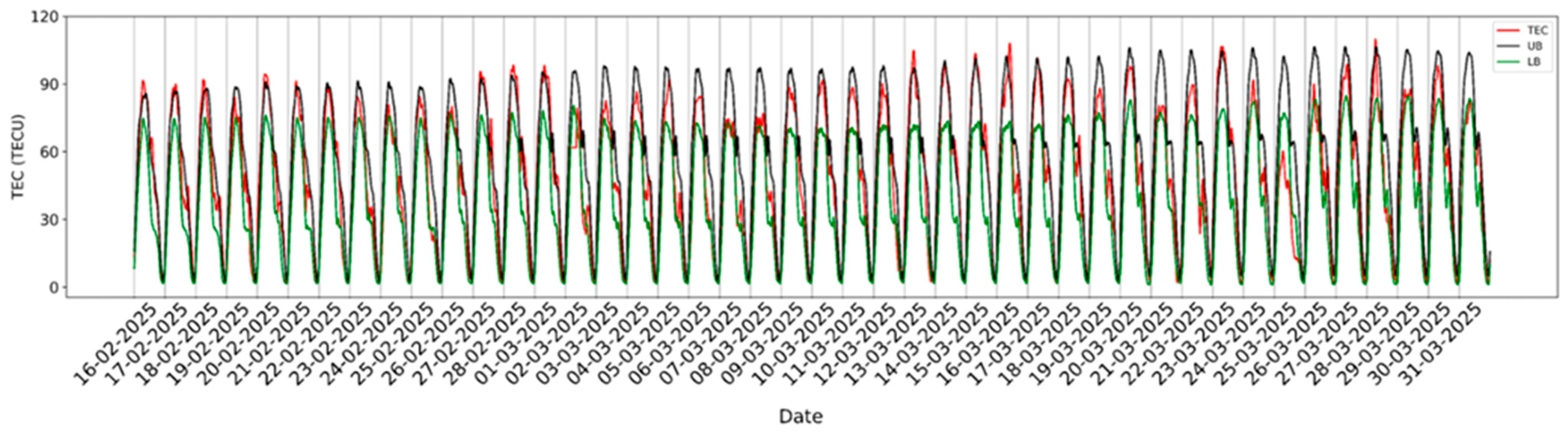
The temporal evolution of vTEC anomalies prior to the Mw 7.7 Myanmar earthquake on 28 March 2025, reveals a distinct and statistically significant pattern of pre-seismic ionospheric perturbations. Figure 3 presents the continuous TEC time series from 16 February to 31 March 2025, recorded at the nearest GNSS station, CMUM, to the earthquake epicenter. This time series is plotted alongside the computed dynamic upper and lower bounds (μ ± 1.34σ), derived from a rolling 15-day window. A clear negative TEC anomaly is observed beginning on 25 March, approximately three days prior to the mainshock, characterized by sustained TEC values falling well below the lower statistical threshold. The magnitude of this depletion reaches approximately 25–30 TECU below the background mean, persisting for nearly 16–18 h before gradually recovering toward background levels by the day of the earthquake. The prolonged and coherent exceedance of the lower statistical envelope indicates that this depletion represents a significant ionospheric disturbance, distinct from normal background variability.

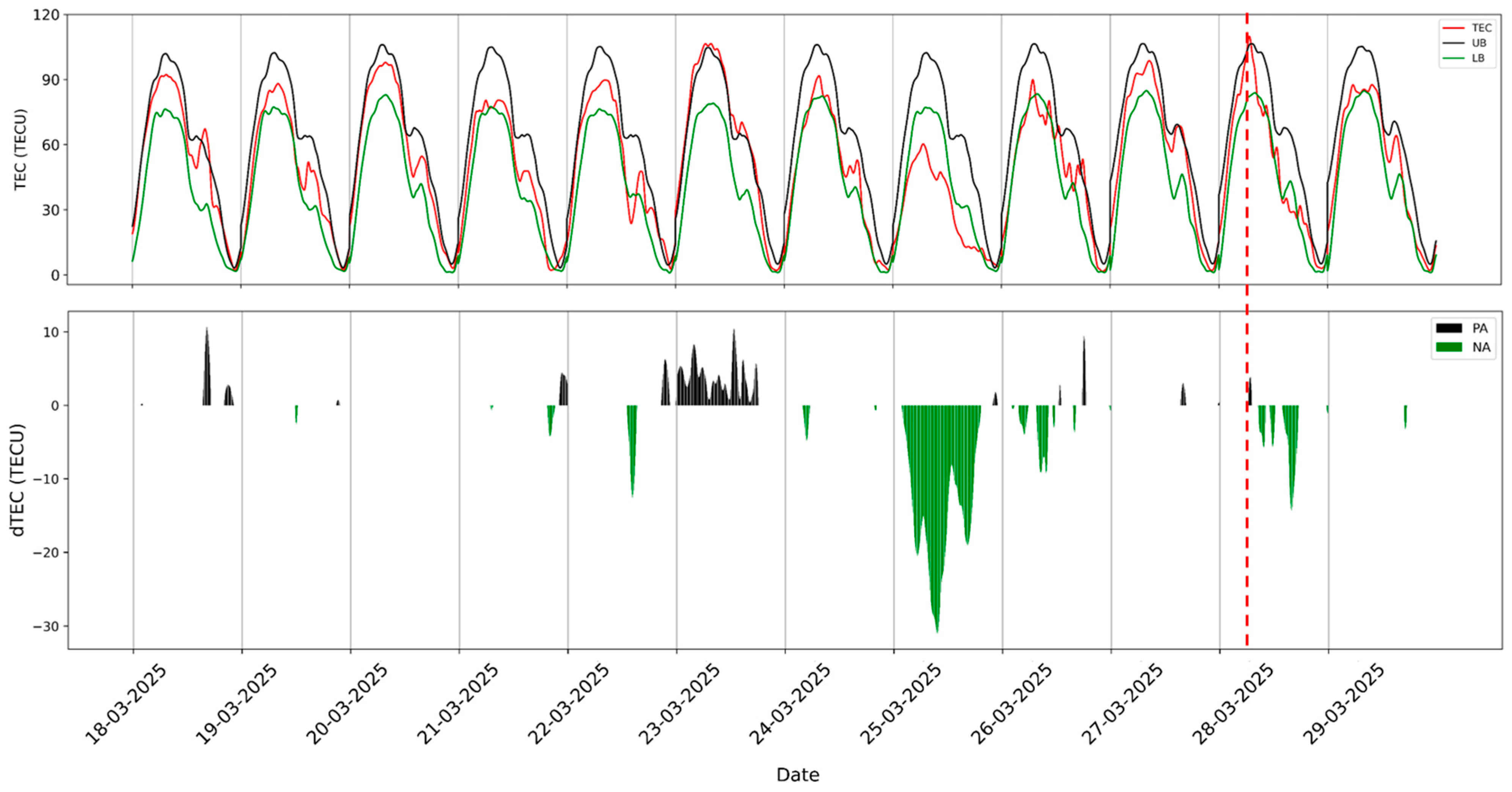
To facilitate an even clearer visualization of the short-term ionospheric dynamics in the immediate lead-up to the earthquake, we focused on a 12-day window from 18 March to 29 March 2025. This subset allowed us to capture fine-scale temporal variations and identify any short-lived disturbances that might be lost in a longer-term view. As shown in Figure 4, the TEC time series (upper panels) exhibits a marked and persistent negative anomaly on 25 March, coincident with the largest departure from background conditions during the study period. The corresponding dTEC plots (lower panels) confirm this behavior, with pronounced negative excursions dominating the period, reaching values close to −30 TECU, while positive deviations remain comparatively weak and sporadic. The spatial and temporal coherence of these negative anomalies across the analyzed stations suggests a regionally organized ionospheric depletion, temporally aligned with the earthquake preparation phase. This behavior supports the interpretation that sustained TEC reductions, rather than enhancements, may serve as a reliable ionospheric manifestation of pre-seismic processes in this event.

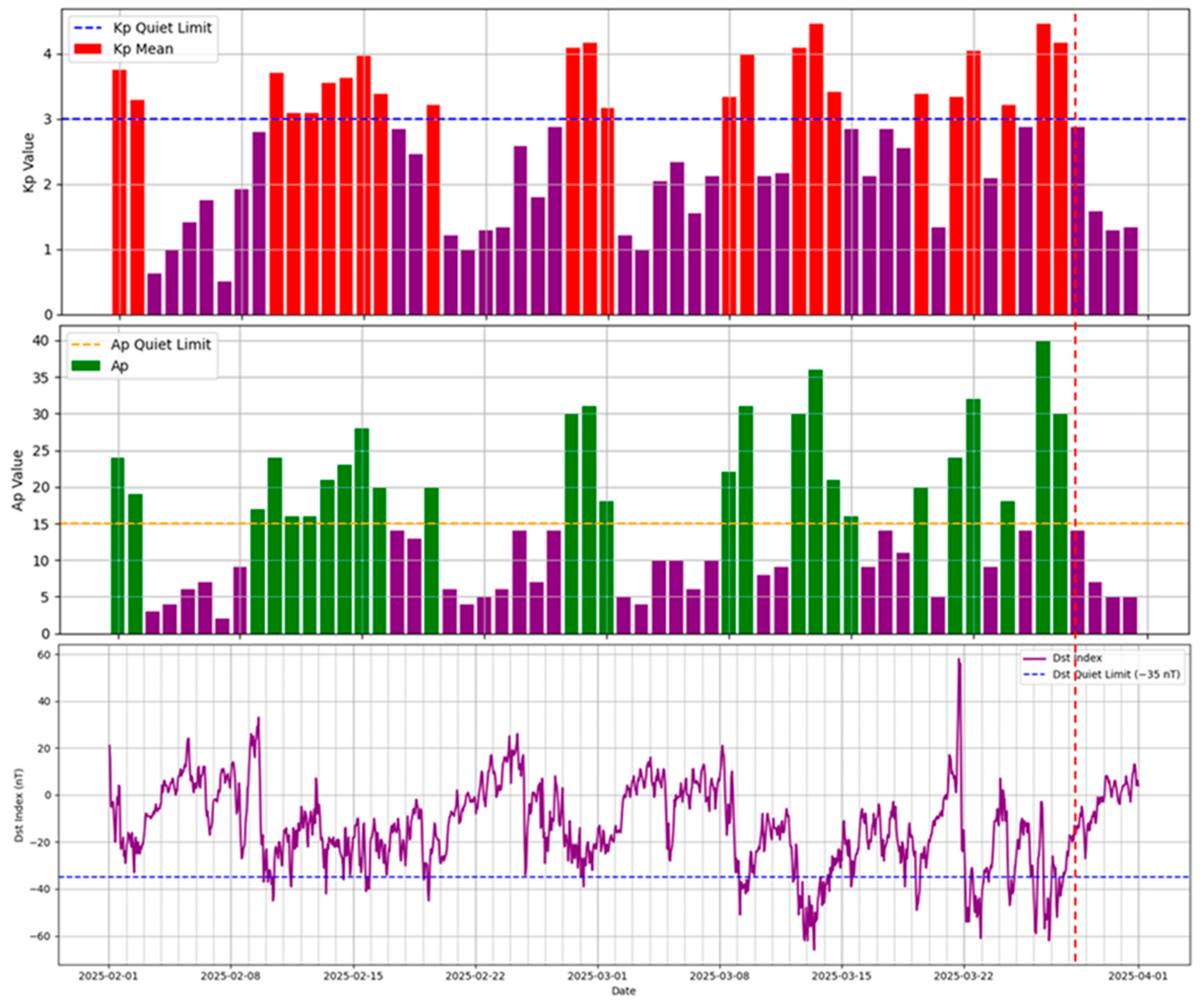
To critically assess whether the observed TEC anomalies could have been influenced by space weather forcing, we examined the planetary geomagnetic indices Kp, Ap, and Dst over the full analysis period from 1 February to 31 March 2025 (Figure 5). Particular attention was given to 25 March, the day on which the strongest TEC anomaly was identified. On 25 March, geomagnetic conditions were distinctly quiet, with Kp values remaining below 3, Ap below 20, and Dst above −35 nT, thresholds that are widely adopted to define magnetically quiet periods. This confirms that the pronounced negative TEC anomaly observed on this day was not driven by external geomagnetic disturbances, thereby excluding space weather activity as the primary cause. In contrast, 26 and 27 March exhibited moderate geomagnetic activity, with Kp values approaching 3.5–4 and Ap increasing to approximately 25–30. Such fluctuations are not uncommon in low- to mid-latitude regions, particularly within or near the equatorial ionospheric anomaly (EIA) belt, where background ionospheric variability can be moderately amplified [59]. Additionally, several days within the study window (19, 21, 22, 24, 26, and 27 March) recorded Ap > 20, Kp > 3, and Dst < −35 nT, reflecting transient geomagnetic perturbations consistent with seasonal ionospheric variability at the latitude of Myanmar (~22° N). However, these geomagnetic disturbances were short-lived and episodic, lacking the temporal persistence and magnitude required to generate the sustained and statistically significant TEC depletion observed on 25 March. Importantly, no comparable TEC anomaly was detected on days with higher geomagnetic activity, further supporting the interpretation that the 25 March event is independent of space weather forcing. Overall, the geomagnetic analysis demonstrates that the prominent TEC depletion on 25 March occurred under magnetically quiet conditions and is therefore more plausibly attributed to lithospheric processes associated with earthquake preparation, reinforcing its significance as a potential seismo-ionospheric precursor.

3.2. IDI and ROTI Variability

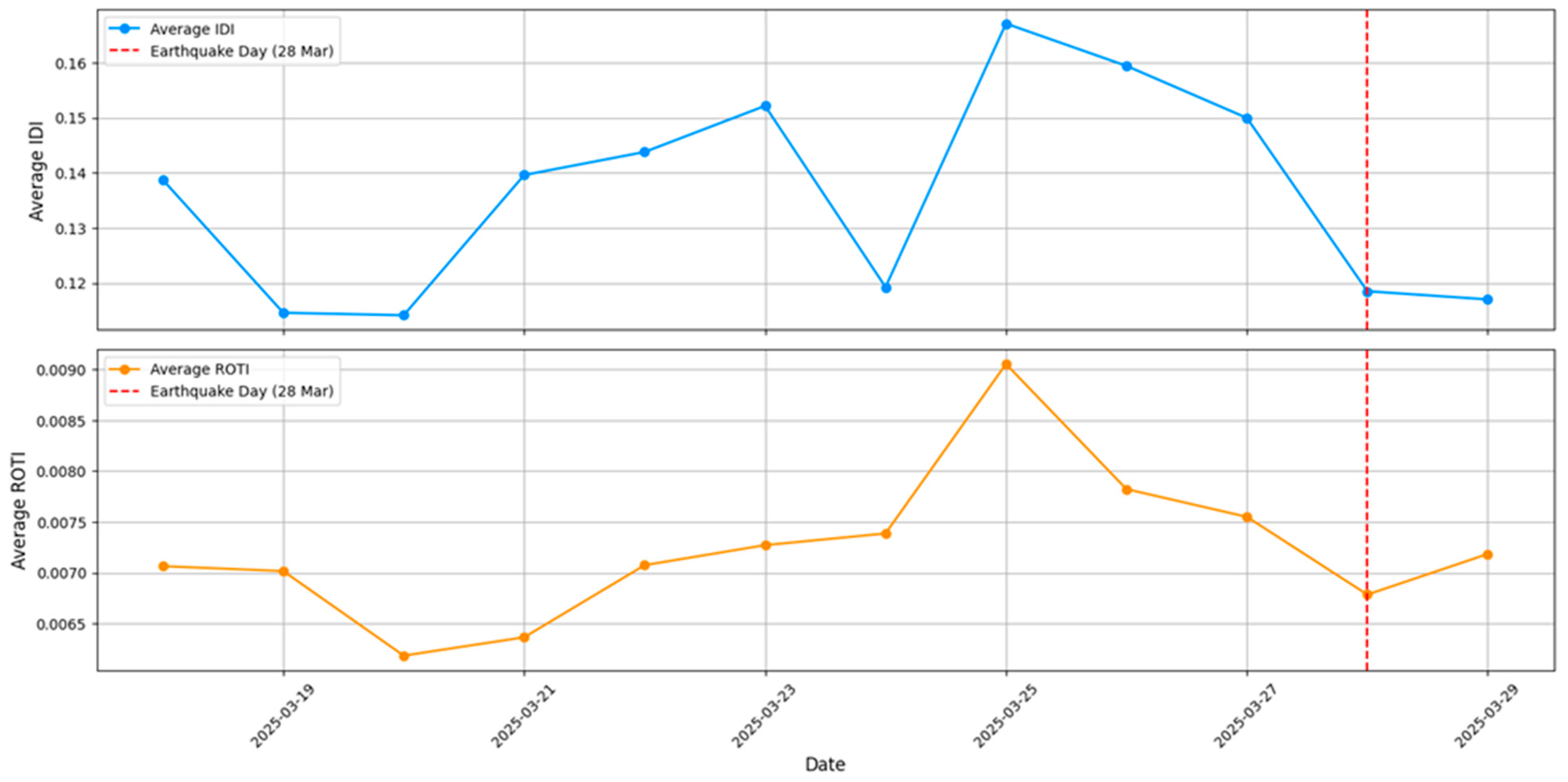
Following the identification of a pronounced negative TEC anomaly on 25 March 2025, the Ionospheric Disturbance Index (IDI) and the Rate of TEC Index (ROTI) were compared to better characterize ionospheric perturbations. These indices were obtained from all 16 GNSS stations used within the study area, enabling us to capture the regional extent of the ionospheric response.

Figure 6 illustrates the daily averaged IDI and ROTI values for the period 18–29 March 2025. A pronounced enhancement in both indices was observed on 25 March, with IDI reaching a maximum value of approximately 0.16, accompanied by a concurrent increase in ROTI to about 0.0090 TECU min⁻¹. The simultaneous elevation of these indices indicates the presence of strong large-scale deviations from the background ionospheric state, together with enhanced short-term TEC variability on this day. Physically, elevated IDI values reflect the magnitude of ionospheric departure from climatological conditions, independent of anomaly polarity, and therefore signify a strongly disturbed ionosphere during the depletion phase. Similarly, increased ROTI values indicate intensified short-term TEC fluctuations, consistent with enhanced ionospheric variability during the same period. Notably, although secondary increases in IDI and ROTI are observed on 21, 22, 26, and 27 March, these days coincide with periods of moderate geomagnetic activity, as shown by the space weather analysis. In contrast, the pronounced IDI–ROTI enhancement on 25 March occurred under geomagnetically quiet conditions, reinforcing its interpretation as a genuine pre-seismic ionospheric disturbance rather than a space weather-driven effect. The concurrence of strong TEC depletion with elevated IDI and ROTI values further supports the presence of a coherent seismo-ionospheric response during the earthquake preparation phase.

3.3. AGW Power-Frequency Distribution

Building upon the observed negative TEC anomaly and the associated IDI–ROTI variability, a dedicated analysis of acoustic–gravity wave (AGW) signatures embedded within the TEC time series was carried out to characterize neutral–ionospheric perturbations during the earthquake preparation phase. AGWs represent upward-propagating atmospheric disturbances capable of modulating ionospheric plasma through ion–neutral coupling and altered transport processes. 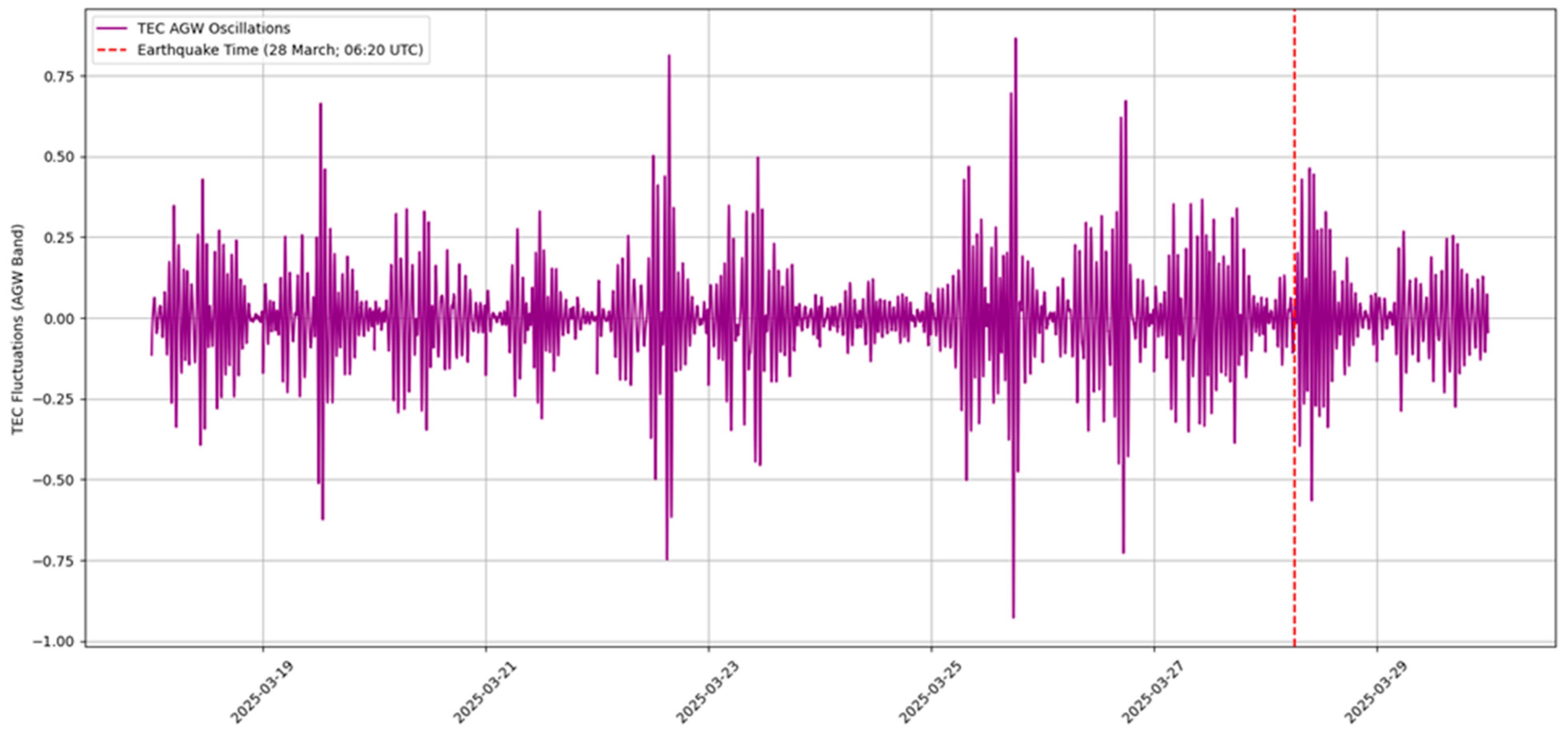Figure 7 shows the AGW-band TEC oscillations, obtained by band-pass filtering the TEC residuals and averaged across all 16 GNSS stations for the period 18–29 March 2025. The time series reveals a clear intensification of AGW activity on 25 March, with oscillation amplitudes reaching approximately 0.7–0.8 TECU, representing the strongest AGW signal observed during the study interval. Enhanced oscillatory activity persisted into 26 March before gradually weakening on 27–28 March, indicating a temporally sustained atmospheric–ionospheric disturbance preceding the mainshock.

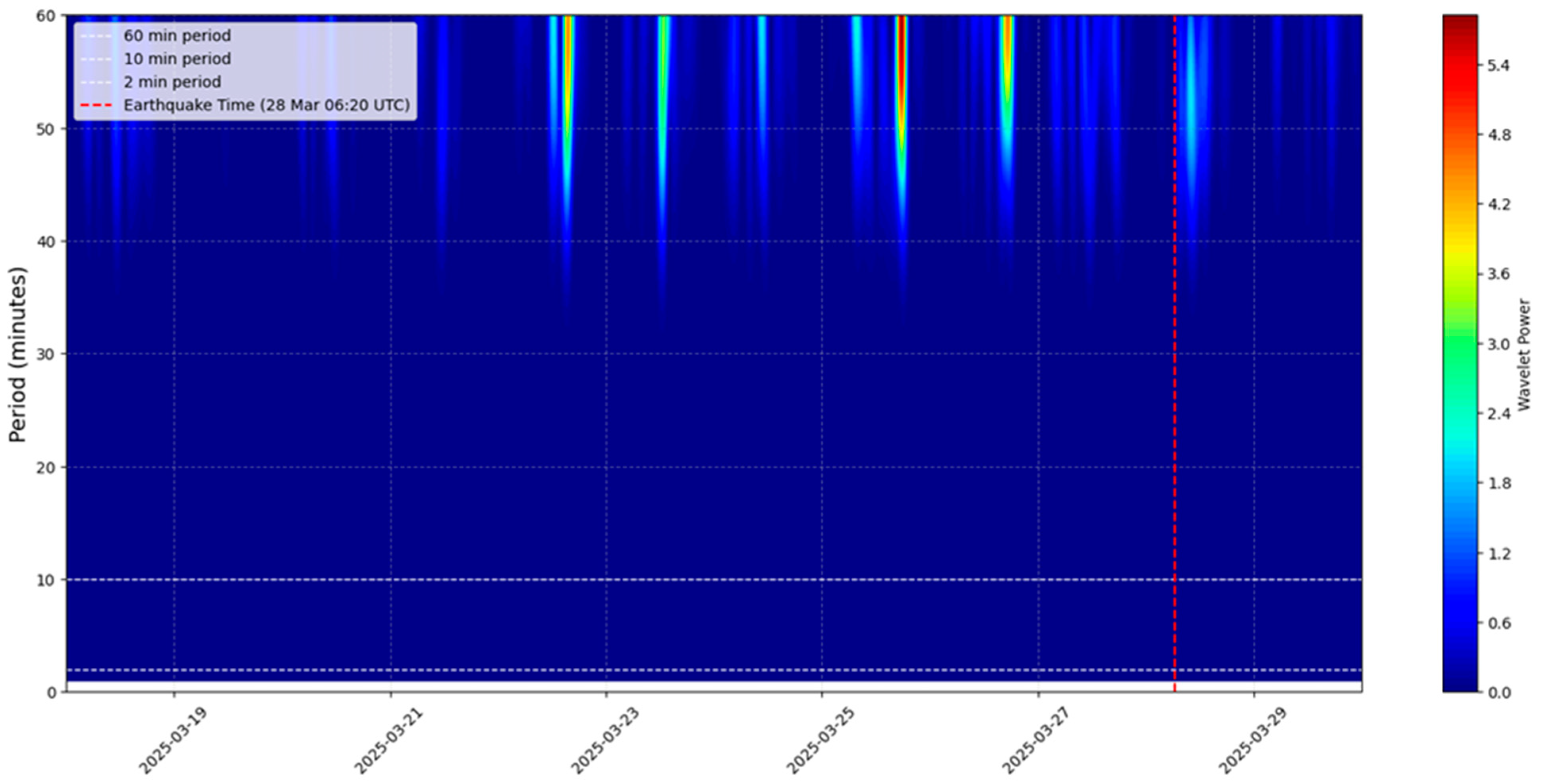
To further examine the frequency characteristics of these oscillations, a continuous wavelet power spectrum analysis was performed (Figure 8). The spectrum reveals dominant energy concentrations within the 40–60 min period band, which is characteristic of AGW activity in the ionospheric F-region. Notably, the strongest and most persistent wavelet power is observed on 25 March, coincident with the maximum TEC depletion and elevated IDI and ROTI values. The presence of sustained power within this longer-period band suggests enhanced upward propagation of AGWs during the pre-seismic phase. Additional, more sporadic AGW power enhancements are visible on 19–22 March and 26–27 March; however, these intervals coincide with periods of moderate geomagnetic activity, as indicated by planetary indices. In contrast, the pronounced AGW intensification on 25 March occurred under geomagnetically quiet conditions, strengthening the interpretation that the observed AGW activity is associated with lithospheric processes rather than externally driven space weather disturbances.

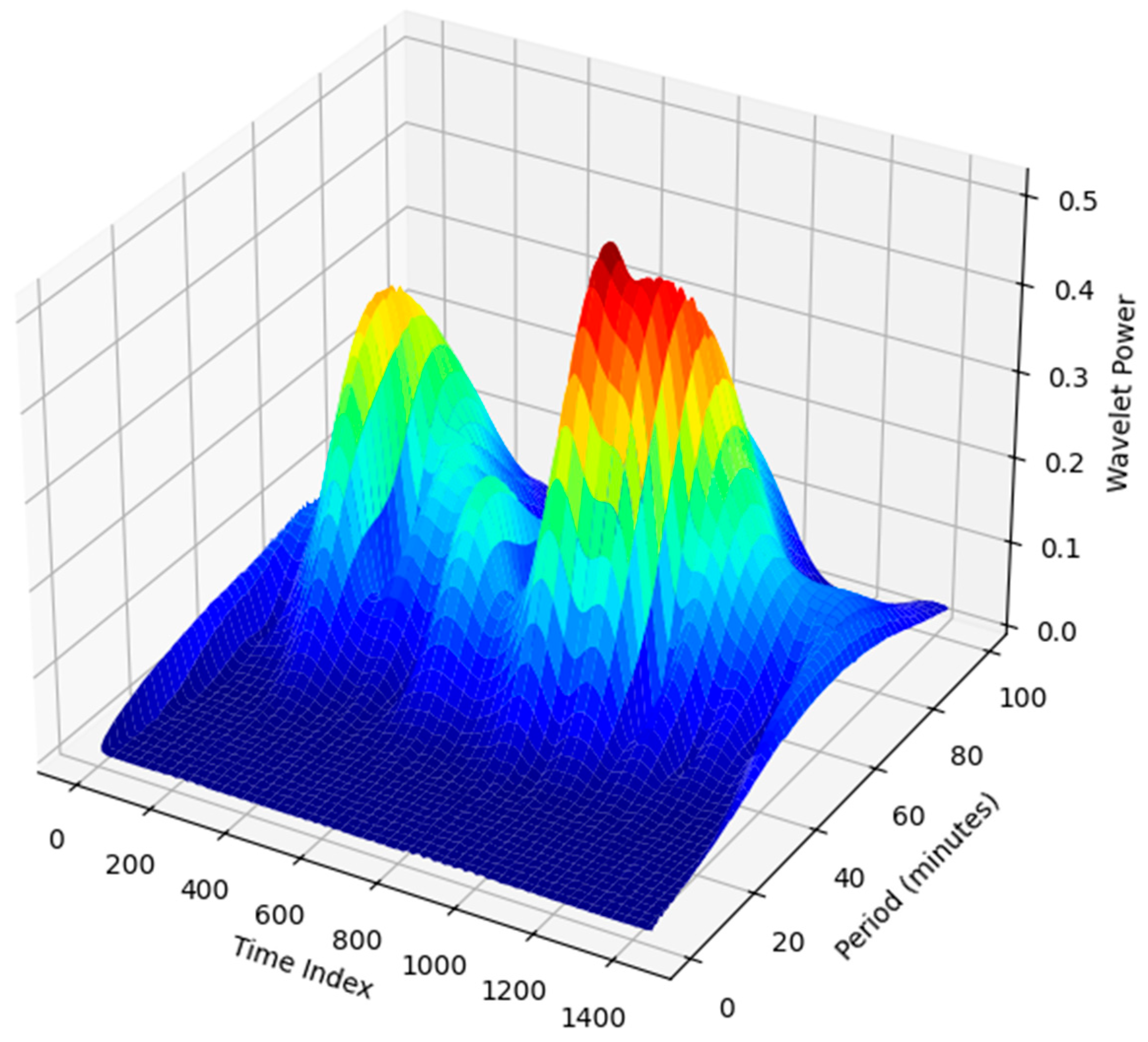
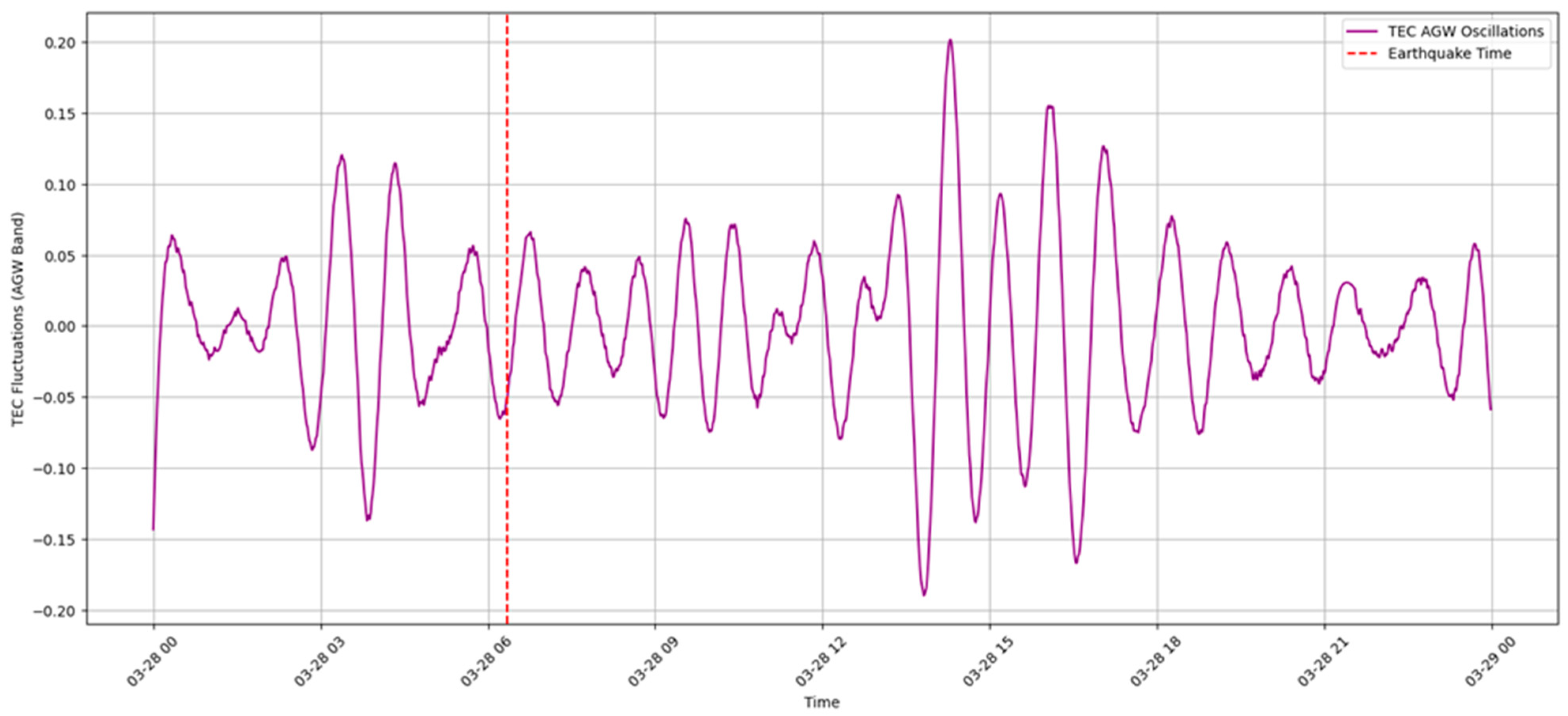
To understand the co-seismic ionospheric response, a three-dimensional wavelet power spectrum analysis was performed for 28 March 2025, the day of the Mw 7.7 Myanmar earthquake. Figure 9 presents the 3D wavelet spectrum derived from TEC residuals, revealing distinct multi-modal enhancements in wavelet power, with dominant periodicities clustering in the 40–80 min band, characteristic of acoustic–gravity wave (AGW) activity in the ionosphere. The earthquake mainshock occurred at 06:20 UTC, and a pronounced enhancement in wavelet power was observed immediately following the rupture time. This post-event intensification indicates the rapid onset of AGW activity triggered by the earthquake, clearly distinguishing the co-seismic response from the pre-seismic AGW signatures identified earlier in the analysis. The concentration of wavelet energy at longer AGW periods suggests efficient upward propagation of atmospheric disturbances during the co-seismic phase. This behavior is further corroborated by the AGW-band TEC oscillation time series shown in Figure 10, which exhibits a sharp increase in oscillation amplitude immediately after 06:20 UTC. The post-mainshock signal is characterized by high-amplitude, coherent oscillations, in contrast to the more gradual pre-seismic variations observed on preceding days. The abrupt onset and temporal alignment with the earthquake origin time provide strong evidence for a direct co-seismic AGW excitation. Such co-seismic AGW signatures are commonly associated with rapid lithospheric energy release during fault rupture, generating pressure perturbations and elastic strain waves that propagate vertically through the neutral atmosphere and couple with ionospheric plasma. The observed oscillations therefore reflect vertical energy transmission from the lithosphere to the ionosphere, resulting in short-term TEC fluctuations immediately following the earthquake.

Overall, the AGW observations reveal a clear temporal distinction between pre-seismic and co-seismic ionospheric responses. While sustained AGW activity on 25 March coincides with the strongest pre-seismic TEC depletion and elevated IDI–ROTI values, the abrupt, high-amplitude oscillations on 28 March represent a distinct co-seismic signature directly linked to earthquake rupture. Together, these results demonstrate that AGWs act as an effective carrier of lithospheric energy into the ionosphere during both the preparation and rupture phases, supporting lithosphere–atmosphere–ionosphere coupling within the studied event.

3.4. Spatial Distribution of TEC Perturbations

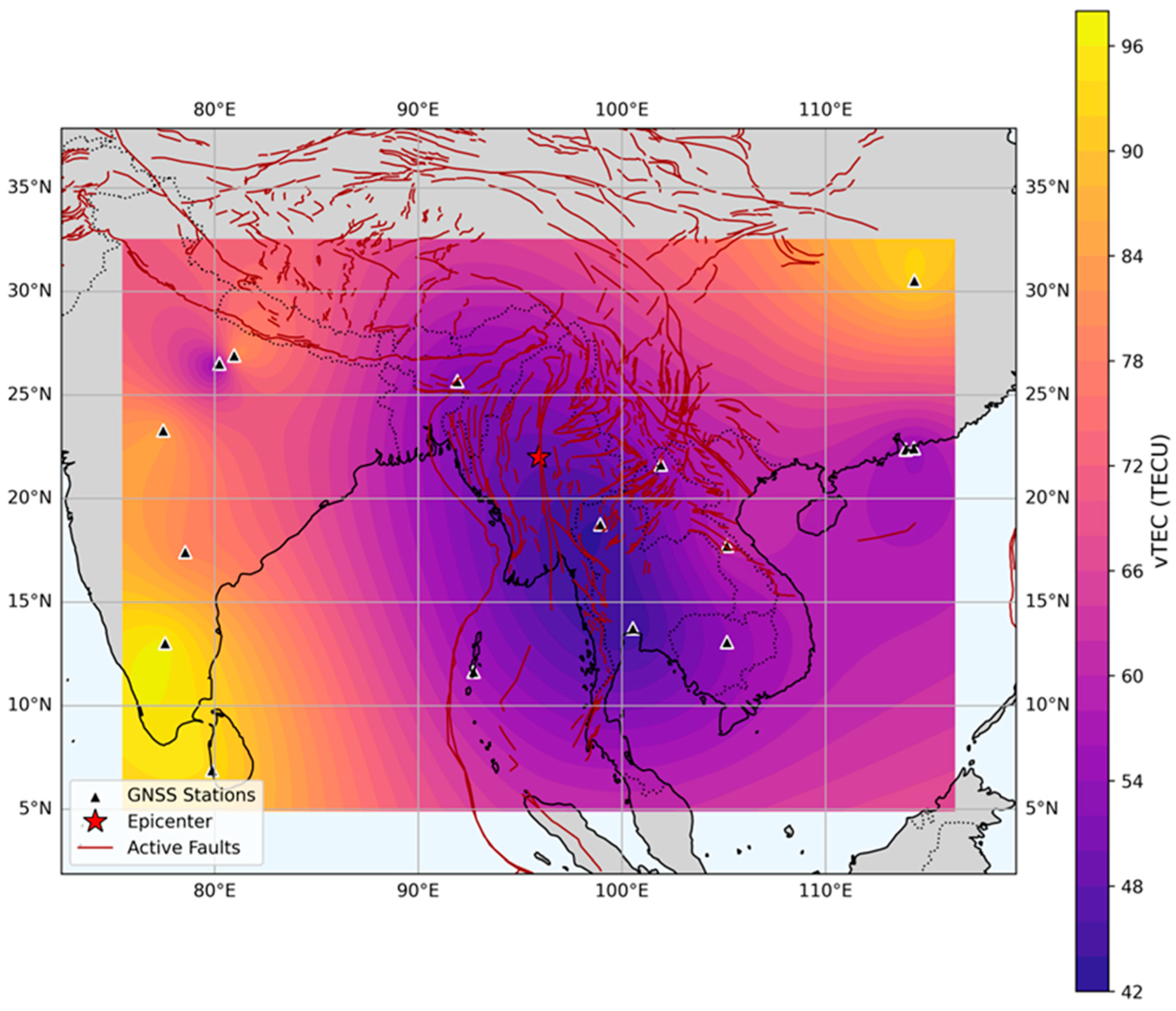
High-resolution spatial maps were generated to elucidate the regional morphology of ionospheric disturbances during the anomaly day (25 March 2025), following the temporal and spectral analyses of TEC anomalies. Ordinary Kriging interpolation was applied to GNSS-derived TEC anomalies to produce continuous spatial distributions across the study region. Particular emphasis was placed on the optimal anomaly time at ~09:60 UTC, corresponding to the epoch when the maximum TEC deviation was observed. At this time, the TEC anomaly reached a magnitude of approximately −31.04 TECU relative to background conditions. The interpolated spatial distribution of TEC anomalies, constructed using data from all 16 GNSS stations, is shown in Figure 11. The map reveals a pronounced region of reduced TEC values centered over Myanmar, with the strongest depletion spatially coincident with the earthquake epicenter (indicated by the red star). Rather than a localized point anomaly, the disturbance manifests as a coherent, laterally extensive depletion zone, spanning several hundred kilometers around the epicentral region. The most intense TEC reductions are concentrated over central Myanmar, while surrounding areas show a gradual transition toward background levels. This spatial structure indicates a coherent ionospheric response consistent with localized lithospheric energy release.

From a physical perspective, the presence of a negative TEC anomaly indicates a substantial reduction in ionospheric electron density relative to the statistical background state. Such depletion is consistent with modified lithosphere–atmosphere–ionosphere coupling processes operating during the earthquake preparation phase. Progressive stress accumulation in the crust can perturb near-surface electrical and atmospheric conditions through mechanisms such as electro-kinetic effects, stress-activated charge carriers, and enhanced gas emission, which collectively influence atmospheric conductivity and electrodynamic coupling. These processes may alter ion–neutral interactions and plasma transport within the lower thermosphere, leading to suppressed upward plasma drift or effective downward redistribution of ionospheric plasma. As plasma is transported to lower altitudes where recombination rates are higher, a net decrease in TEC can result. The spatial coherence of the TEC depletion, extending several hundred kilometers around the epicentral region, reflects the regional scale of the underlying stress field rather than localized ionospheric noise. This spatial pattern temporally coincides with the negative excursions in the TEC time series, elevated IDI values, enhanced ROTI, and intensified AGW activity identified in the temporal and spectral analyses. The concurrence of these independent parameters supports a physically consistent interpretation of the observed ionospheric response. In contrast, regions outside the affected zone exhibit TEC values close to background levels, providing a reference that highlights the localized nature of the disturbance. The strongest TEC gradients are concentrated near the epicenter, where stress accumulation and associated coupling processes are expected to be most pronounced, supporting the interpretation of the 25 March TEC depletion as a seismo-ionospheric precursor to the earthquake. The spatial coherence and epicentral alignment of the TEC depletion zone argue against localized ionospheric noise and instead point to a regional-scale response to stress accumulation within the underlying lithosphere.

3.5. b-Value and Seismic Hazard Mapping

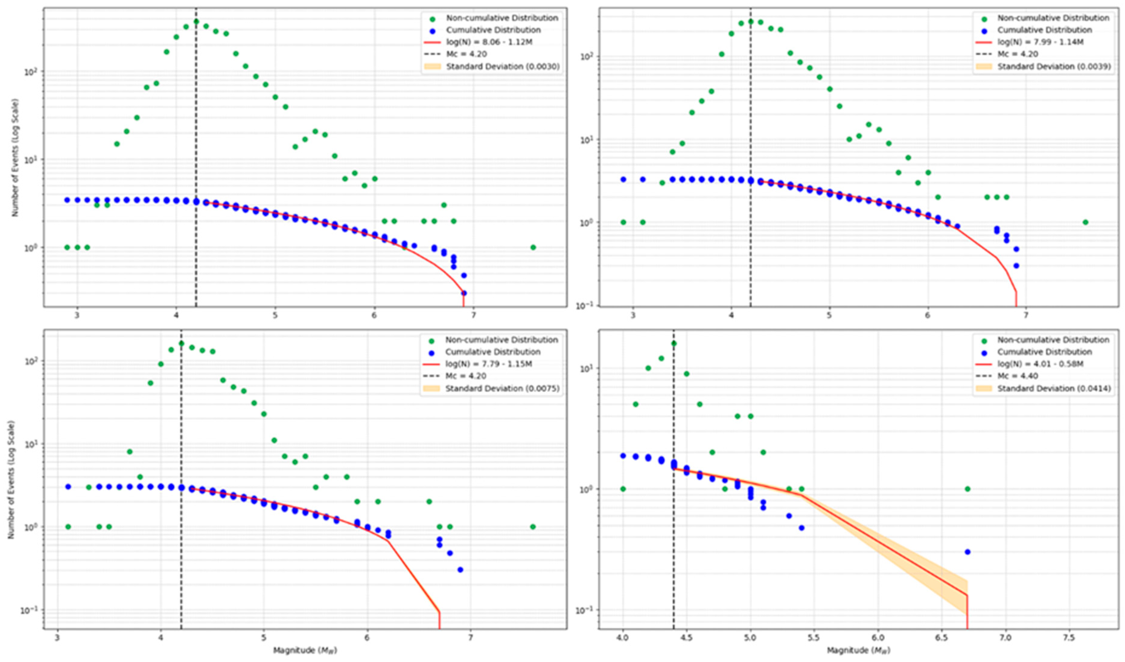
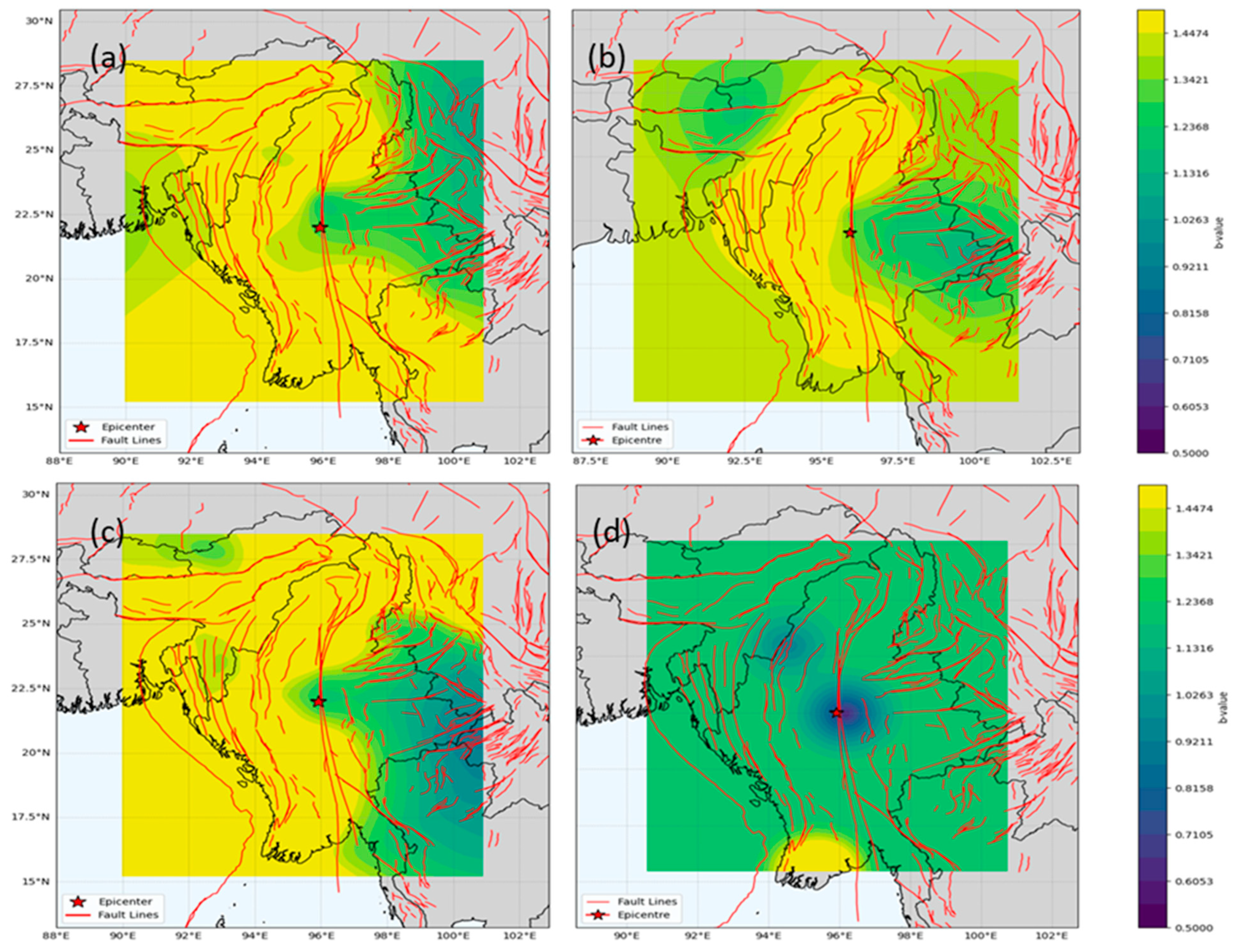
The comprehensive analysis of b-values derived from seismic event distributions provides crucial insights into seismic hazard conditions preceding significant earthquakes in the Myanmar region. The temporal analysis conducted across periods of 30 years, 20 years, 10 years, and the recent 6-month interval highlights distinct and significant patterns. The b-value calculations (Figure 12) reveal a consistent decline in b-value leading up to the mainshock, with the lowest values observed in the 6-month window preceding the earthquake. Specifically, b-values decreased from approximately 1.12 (30-year window) to 0.58 (6-month window), highlighting a potential period of stress accumulation in the crust. This trend is consistent with seismo-tectonic studies, where lower b-values are often indicative of increased stress heterogeneity and elevated earthquake potential.

Spatial analysis of seismic b-values across varying temporal intervals (Figure 13) reveals a clear progression in stress accumulation patterns in the Myanmar region. Over the 30-year interval (panel a), a broadly homogeneous and moderately high b-value distribution was observed, indicating generally balanced seismicity and moderate levels of tectonic stress accumulation. During the subsequent 20-year interval (panel b), subtle variations emerged, with slightly decreased b-values appearing near the eventual epicenter, suggesting the initial stages of localized stress concentration. As the analysis interval narrowed to the past 10 years (panel c), the low b-value region became increasingly prominent around the epicentral zone, signaling a notable increase in tectonic stress accumulation and heightened seismic potential. In the immediate 6-month interval leading to the earthquake (panel d), the b-value map displayed a distinct, sharply delineated region of extremely low values surrounding the March 2025 epicenter. This pronounced anomaly signifies intense and highly localized tectonic stress, clearly indicating imminent seismic activity.

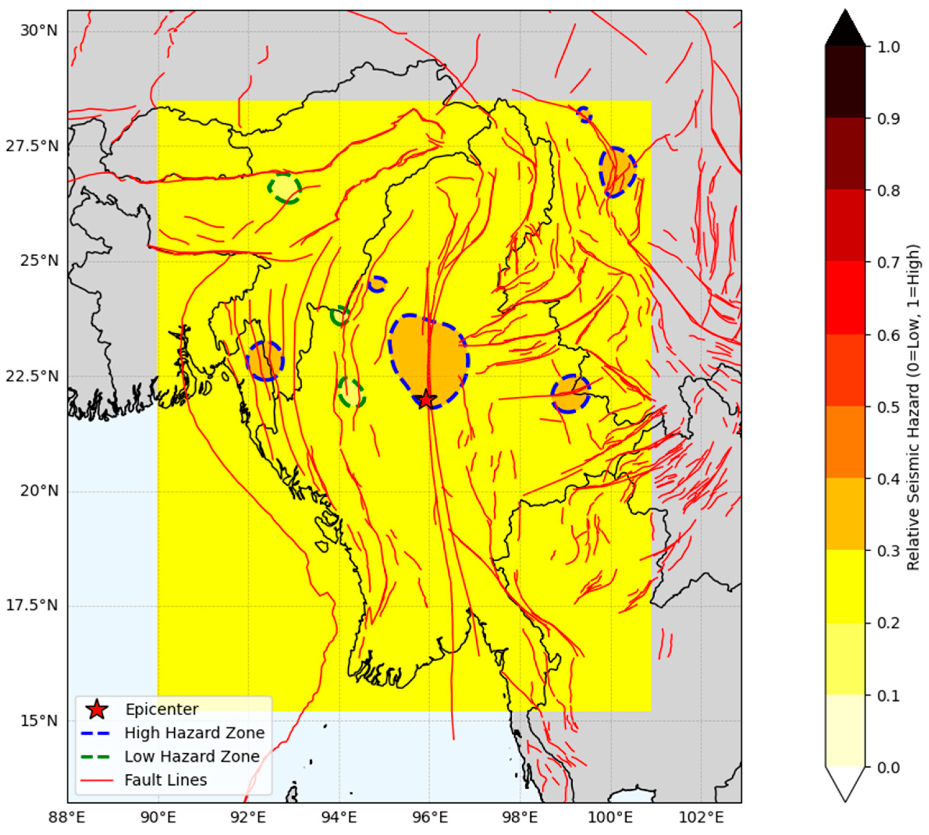
The RSHI spatial analysis, as shown in Figure 14, provides a robust quantitative assessment of seismic risk, effectively complementing the b-value insights. Notably, the high-hazard zones coincide closely with areas of significantly reduced b-values in the short-term (6-month) assessment. This strong spatial correlation underscores the reliability of integrated seismic risk evaluations combining b-value and RSHI methodologies. Further enhancement of this analysis is achieved through integration with previously identified ionospheric TEC depletion. Significantly, the zones marked by prominent pre-seismic TEC depletion overlap consistently with the identified low b-value and high seismic hazard regions, especially pronounced in the immediate vicinity of the earthquake epicenter during the 6-month analysis window. Such overlaps validate the hypothesis that simultaneous ionospheric and crustal anomalies are reliable indicators of impending seismic activities.

The strong correlation among low b-values, TEC depletion, and elevated seismic hazard index zones reflects a physically coherent scenario of progressive tectonic stress accumulation and crustal deformation. Geologically, these identified zones align with major fault structures known for historical seismic activities, further reinforcing the credibility of these observations. These consistent results advocate for the adoption of integrated seismo-ionospheric methodologies in regional seismic hazard assessment and predictive modeling.

3.6. Joint Distribution and Correlation Analysis

The joint distribution of seismic b-values and interpolated vTEC reveals important insights into the coupling between lithospheric stress accumulation and ionospheric disturbances during the earthquake preparation phase. To examine this relationship comprehensively, three complementary visualization approaches were employed: kernel density estimation (KDE), two-dimensional histogram analysis, and quadrant-based classification. Together, these methods allow both continuous and discrete characterization of stress–ionosphere coupling within the study region.

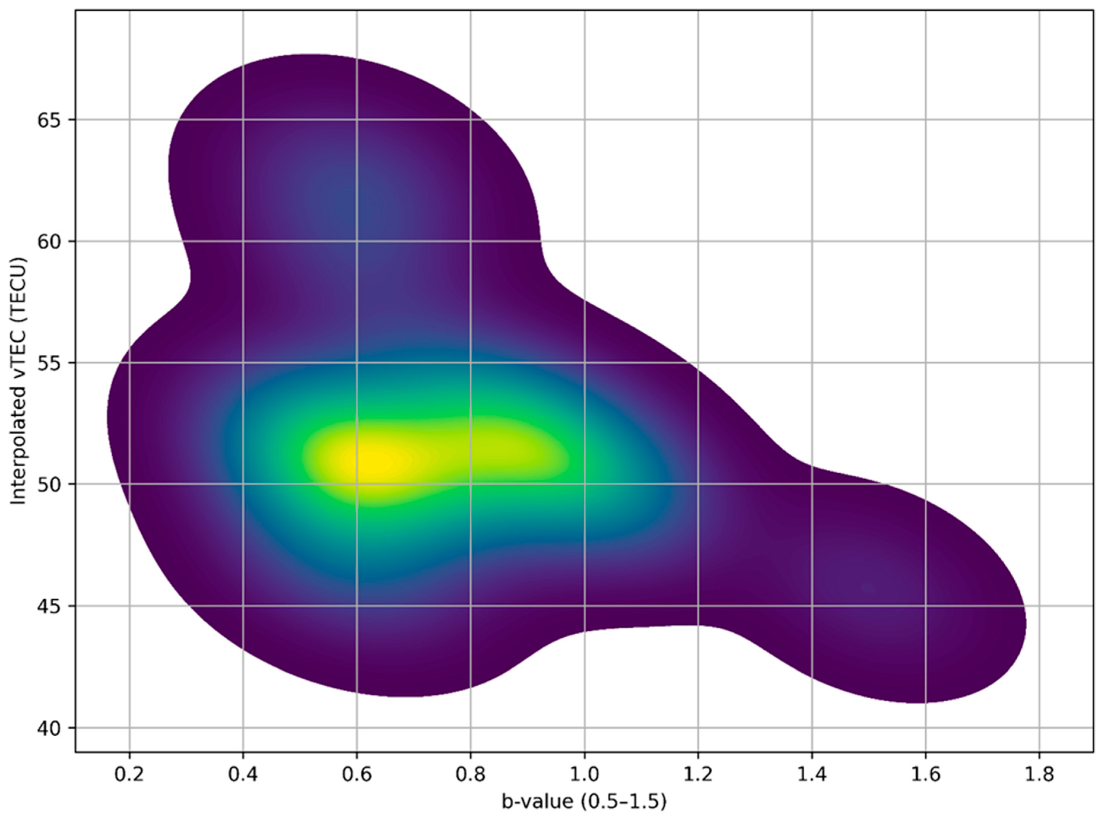
The KDE plot (Figure 15) reveals a pronounced density maximum concentrated within the low b-value range (~0.55–0.75) and lower vTEC values (~48–52 TECU). This dominant density core indicates that the most frequent joint occurrence corresponds to regions characterized by elevated crustal stress, as inferred from reduced b-values, accompanied by ionospheric electron density depletion. The density smoothly decays toward higher b-values and higher vTEC, suggesting that as seismic conditions become more stable, ionospheric perturbations occur less frequently. The asymmetric structure of the KDE distribution reveals a preferential coupling between zones of stress concentration and suppressed ionospheric electron content, a relationship first systematically identified by Nayak et al. [14]. Their study demonstrated that negative TEC anomalies are closely associated with regions characterized by low b-values, indicating enhanced stress accumulation prior to seismic rupture.

The two-dimensional histogram analysis (Supplementary Figure S1) further corroborates the KDE results by discretizing the joint parameter space into frequency bins. The highest-density bins are located predominantly in the low b-value–low vTEC domain, confirming that this regime represents the most statistically significant coupling between seismic and ionospheric parameters. In contrast, bins corresponding to higher b-values show substantially lower population densities, indicating that relatively stable crustal conditions are less commonly associated with marked ionospheric variability. This distribution pattern supports the interpretation that stress localization plays a primary role in modulating ionospheric conditions prior to an earthquake.

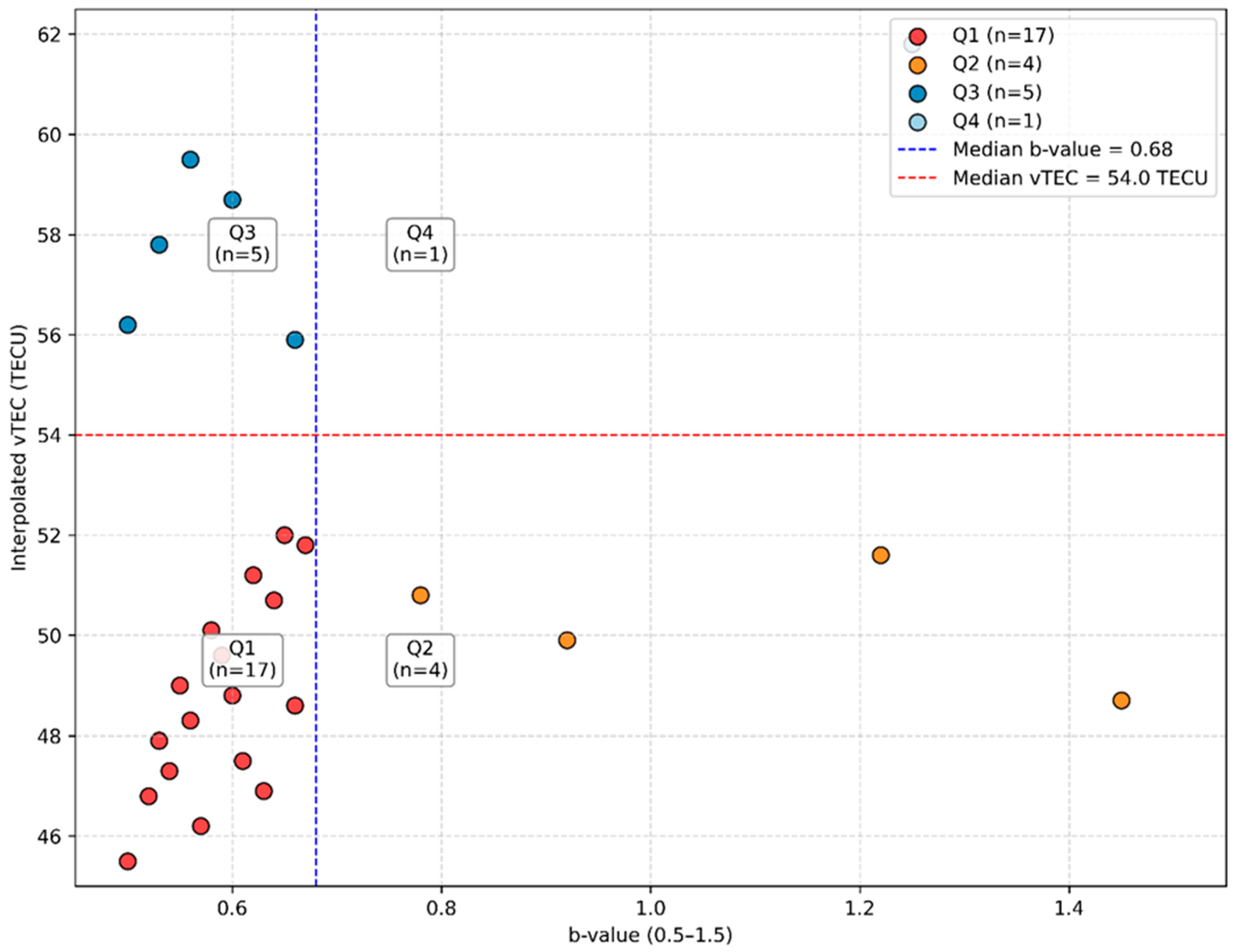
To formalize the joint distribution interpretation, a quadrant-based classification was applied, dividing the b–vTEC parameter space into four distinct domains using the median values of both parameters as thresholds. The resulting scatter plot (Figure 16) partitions the b–vTEC parameter space into four distinct domains that reflect different stress-controlled ionospheric response regimes. Quadrant Q1, defined by low b-values and low vTEC, contains the highest concentration of observations (n = 17), indicating that this regime most consistently characterizes the coupled lithospheric–ionospheric state during the earthquake preparation phase. Low b-values imply elevated stress concentration and increased heterogeneity within the crust, while the simultaneous reduction in vTEC reflects a net depletion of ionospheric plasma. The dominance of Q1 therefore suggests that regions undergoing intensified stress accumulation are preferentially associated with modified plasma transport and enhanced recombination processes, resulting in reduced ionospheric electron content. Quadrant Q2 (high b-value, low vTEC) contains a limited number of points, indicating that ionospheric depletion can occur even under relatively distributed or lower stress conditions, but with substantially reduced occurrence. This regime may reflect background ionospheric variability or secondary coupling effects not directly driven by strong stress localization. Quadrant Q3 (low b-value, high vTEC) represents regions where stress accumulation is present but has not manifested as ionospheric depletion, potentially due to spatial variations in lithospheric structure, stress orientation, or inefficiencies in vertical atmosphere–ionosphere coupling. Quadrant Q4 (high b-value, high vTEC) is sparsely populated, suggesting that areas characterized by both stable seismic conditions and enhanced ionospheric electron content are least representative of the physical processes governing earthquake preparation.

Overall, the integration of KDE, 2D histogram analysis, and quadrant-based classification provides a comprehensive understanding of the stress–ionosphere relationship during the earthquake preparation phase. The consistent clustering of points in low b-value and reduced vTEC regions across all three visualization methods underscores the significance of stress accumulation as a driver of pre-earthquake ionospheric anomalies. These findings highlight the importance of adopting a multi-parametric approach to earthquake precursor research, combining seismological and ionospheric observations to improve detection and monitoring of earthquake preparation processes.

4. Discussion

This study integrates multiple geophysical parameters to investigate the seismo-ionospheric response associated with the Mw 7.7 Myanmar earthquake on 28 March 2025, including GNSS-based TEC anomalies, IDI and ROTI, AGW signatures, b-value temporal and spatial variations, RSHI mapping, and KDE-based coupling analysis. The results reveal a robust lithosphere–ionosphere coupling process unfolding during the earthquake preparation phase.

Table 2. Chronological summary of key observations during the earthquake preparation and co-seismic phases (Myanmar Mw 7.7 earthquake).

Phase	Parameter	Observation Period	Key Findings	Interpretation
1. Long-Term Stress Accumulation	b-value (Temporal)	30 years to 6 months	Progressive decline from ~1.12 to ~0.58	Indicates increasing stress concentration and crustal heterogeneity associated with earthquake preparation
2. Spatial Stress Localization	b-value (Spatial)	6-month window	Low near epicenter	Highlights localized stress accumulation spatially coincident with ionospheric disturbance region
3. Lithosphere–Ionosphere Coupling Initiation	TEC Anomaly (vTEC)	25 March 2025	Strong negative TEC anomaly (dTEC ≈ −31 TECU)	Regional ionospheric depletion linked to stress accumulation; precursor emergence
4. Ionospheric Plasma Irregularities	IDI and ROTI	25 March 2025	IDI ≈ 0.16; ROTI ≈ 0.0090 TECU/min	Enhanced large-scale ionospheric disturbance and small-scale plasma irregularities consistent with stress-related ionospheric modulation
5. Pre-Seismic AGWs	AGW (Pre-Seismic)	25 March 2025	~0.75 TECU amplitude	Upward-propagating AGWs indicating vertical energy transfer from lithospheric stress
6. Co-Seismic Response	AGW (Co-Seismic)	28 March 2025, ~06:20 UTC	Immediate post-mainshock AGW intensification	Direct ionospheric response to seismic rupture and rapid energy release
7. Seismic Hazard Confirmation	RSHI	6-month window	Peaks near the epicenter	Confirms elevated seismic hazard aligning with low b-value and TEC depletion zones
8. Statistical Coupling Validation	KDE and Quadrant-based Classification	25 March 2025	Dominant clustering in Q1 (low b, low vTEC)	Statistically confirms lithosphere–ionosphere coupling through stress-associated ionospheric depletion

, presented below, summarizes the sequential evolution of key ionospheric and seismic parameters, organized chronologically to reflect the physical progression of earthquake preparation.

The earthquake preparation process initiates deep within the lithosphere through long-term stress accumulation, manifested as a temporal decrease in the seismic b-value from 1.12 to 0.58. This decline reflects a growing dominance of large-magnitude seismic events as the crust becomes increasingly brittle, a physical process consistent with the asperity model and stress corrosion mechanisms [60,61]. As stress localizes near the epicenter, spatial b-value mapping reveals the emergence of low b-value zones overlapping the future rupture area, marking regions of heightened stress heterogeneity. This stress accumulation triggers electromagnetic emissions (piezoelectric and electro-kinetic effects) and mechanical energy release, including the generation of AGWs, that propagate vertically through the neutral atmosphere. These AGWs modulate atmospheric density and ionospheric plasma transport, leading to observable perturbations in the TEC. On 25 March, three days before the mainshock, a significant negative TEC anomaly (dTEC ≈ −31 TECU) emerged under geomagnetically quiet conditions, consistent with observations from other major earthquakes [7,45,62,63]. Simultaneous peaks in IDI and ROTI indicate the presence of both enhanced large-scale ionospheric disturbances and intensified small-scale plasma irregularities, reflecting disturbed plasma dynamics rather than electron density enhancement, and are consistent with AGW-driven ionospheric modulation [64,65,66]. The pre-seismic AGW activity observed on 25 March, with amplitudes reaching ~0.75 TECU, highlights the dynamic energy transfer from the crust to the ionosphere, aligning with the findings by Rolland et al. [67] and Astafyeva et al. [68]. The subsequent co-seismic AGW burst immediately following the earthquake at 06:20 UTC on 28 March reinforces the dual role of AGWs as both precursors and immediate responses to seismic rupture. Co-seismic ionospheric disturbances are often short-lived and directionally dependent, which may limit their detectability in TEC-based observations despite their physical occurrence. Spatially, the TEC depletion zone coincides with the low b-value and high RSHI regions, underscoring the physical connection between stress accumulation in the crust and ionospheric disturbances above. Although moderate geomagnetic disturbances were observed on several days (19, 21, 22, 24, 26, and 27 March), these were transient and did not produce sustained TEC anomalies comparable to the pronounced depletion observed on 25 March. Notably, the 25 March anomaly occurred under geomagnetically quiet conditions and exhibited strong temporal persistence along with consistent enhancements in IDI, ROTI, and AGW activity. This multi-parameter coherence distinguishes it from background ionospheric variability and supports a seismogenic origin. Nevertheless, background ionospheric conditions may influence anomaly detection in some cases, and careful geomagnetic filtering remains essential. Furthermore, while the proposed multi-parameter framework demonstrates strong potential, its broader applicability should be validated across multiple earthquake events and diverse ionospheric conditions. This overlap supports the LAIC hypothesis and reinforces the importance of monitoring both seismic and ionospheric parameters. The KDE-based coupling analysis further validates this relationship by revealing a dominant cluster in the low-b, low-vTEC quadrant, statistically confirming the physical link between lithospheric stress accumulation and pre-seismic ionospheric depletion.

Physically, this progression from deep crustal stress accumulation, through stress localization, to atmospheric–ionospheric coupling supports a multi-scale vertical energy transfer mechanism. Crustal deformation generates both mechanical (AGWs) and electromagnetic emissions that propagate upward, modulating the ionosphere’s electron density and creating observable TEC precursors. This dynamic process aligns with the LAIC framework [27] and highlights the interconnected nature of earthquake preparation across multiple geophysical domains. While this study integrates a robust suite of parameters, limitations remain, including GNSS station density, temporal resolution, and potential unmodeled lower atmospheric or anthropogenic factors. Future studies should integrate multi-GNSS constellations [69], ionosonde measurements [70], and InSAR data [71] to improve spatial resolution and cross-validate ionospheric precursors. Thus, this study demonstrates that a physics-based, multi-parameter approach linking seismic b-values, AGWs, TEC anomalies, and hazard mapping provides a powerful tool for earthquake precursor detection. This integrated methodology enhances our understanding of earthquake preparation processes and underscores the potential of real-time ionospheric monitoring as part of operational early warning systems.

5. Conclusions

The results demonstrate a consistent multi-parameter seismo-ionospheric response to the Mw 7.7 Myanmar earthquake, highlighted by the integration of TEC anomalies, IDI and ROTI variability, AGW signatures, b-value temporal and spatial trends, RSHI mapping, and KDE-based coupling analysis, underscoring the importance of LAIC processes during the earthquake preparation phase. The key conclusions are as follows:

• Significant TEC anomalies were observed approximately three days prior to the earthquake, characterized by a pronounced negative TEC anomaly (dTEC ≈ −31 TECU). This depletion occurred under geomagnetically quiet conditions, reinforcing its lithospheric origin and its association with the earthquake preparation phase.
• IDI and ROTI analyses revealed simultaneous peaks on 25 March, indicating enhanced large-scale ionospheric disturbances and intensified small-scale plasma irregularities. These signatures reflect disturbed plasma transport and ion–neutral coupling processes rather than electron density enhancement, highlighting the role of AGWs and pre-seismic plasma instabilities in ionospheric precursor detection.
• AGW analysis demonstrated strong pre-seismic oscillations on 25 March, with amplitudes reaching ~0.75 TECU, followed by a sharp co-seismic AGW intensification immediately after the mainshock at 06:20 UTC on 28 March. These results confirm the dual role of AGWs as indicators of both pre-seismic energy transfer and co-seismic lithospheric rupture.
• b-value analysis revealed a consistent decline from ~1.12 to ~0.58 across the 30-year to 6-month time windows, indicating progressive crustal stress accumulation. Spatial b-value mapping identified well-defined low b-value zones tightly clustered around the earthquake epicenter, consistent with localized stress concentration.
• RSHI mapping identified high seismic hazard zones overlapping both the low b-value regions and the TEC depletion area, confirming the convergence of independent lithospheric and ionospheric indicators as reliable markers of earthquake preparation.
• KDE-based coupling analysis demonstrated a dominant clustering in the low-b, low-vTEC quadrant (Q1), statistically validating the physical linkage between intensified crustal stress accumulation and pre-seismic ionospheric depletion.

Collectively, these findings demonstrate the effectiveness of integrating seismic, ionospheric, and atmospheric parameters into a unified earthquake precursor detection framework. The strong temporal and spatial coherence among TEC depletion, IDI/ROTI variability, AGW activity, b-value evolution, RSHI mapping, and KDE-based statistical coupling highlights the potential of real-time, multi-parameter monitoring for improving short-term earthquake forecasting. This integrated approach establishes the Myanmar Mw 7.7 earthquake as a benchmark case for validating LAIC-driven precursor mechanisms. Future research should focus on operational implementation using real-time GNSS networks, multi-constellation observations, and atmospheric monitoring systems, as well as extending this framework to other tectonically active regions to enhance regional and global earthquake hazard assessment.