Author Contributions
Conceptualization, X.Z. and C.Z.; Methodology, X.Z., C.Z. and H.C.; Validation, X.Z., G.Z. and H.C.; Formal Analysis, X.Z., G.Z. and H.C.; Investigation, H.C. and G.G.; Data Curation, X.Z., G.Z., C.Z., H.C. and G.G.; Writing—Original Draft Preparation, X.Z.; Writing—Review and Editing, G.Z., C.Z. and H.C.; Visualization, X.Z. and H.C.; Supervision, G.Z. and C.Z.; Project Administration, C.Z.; Funding Acquisition, G.Z. and C.Z. All authors have read and agreed to the published version of the manuscript.
Figure 1.
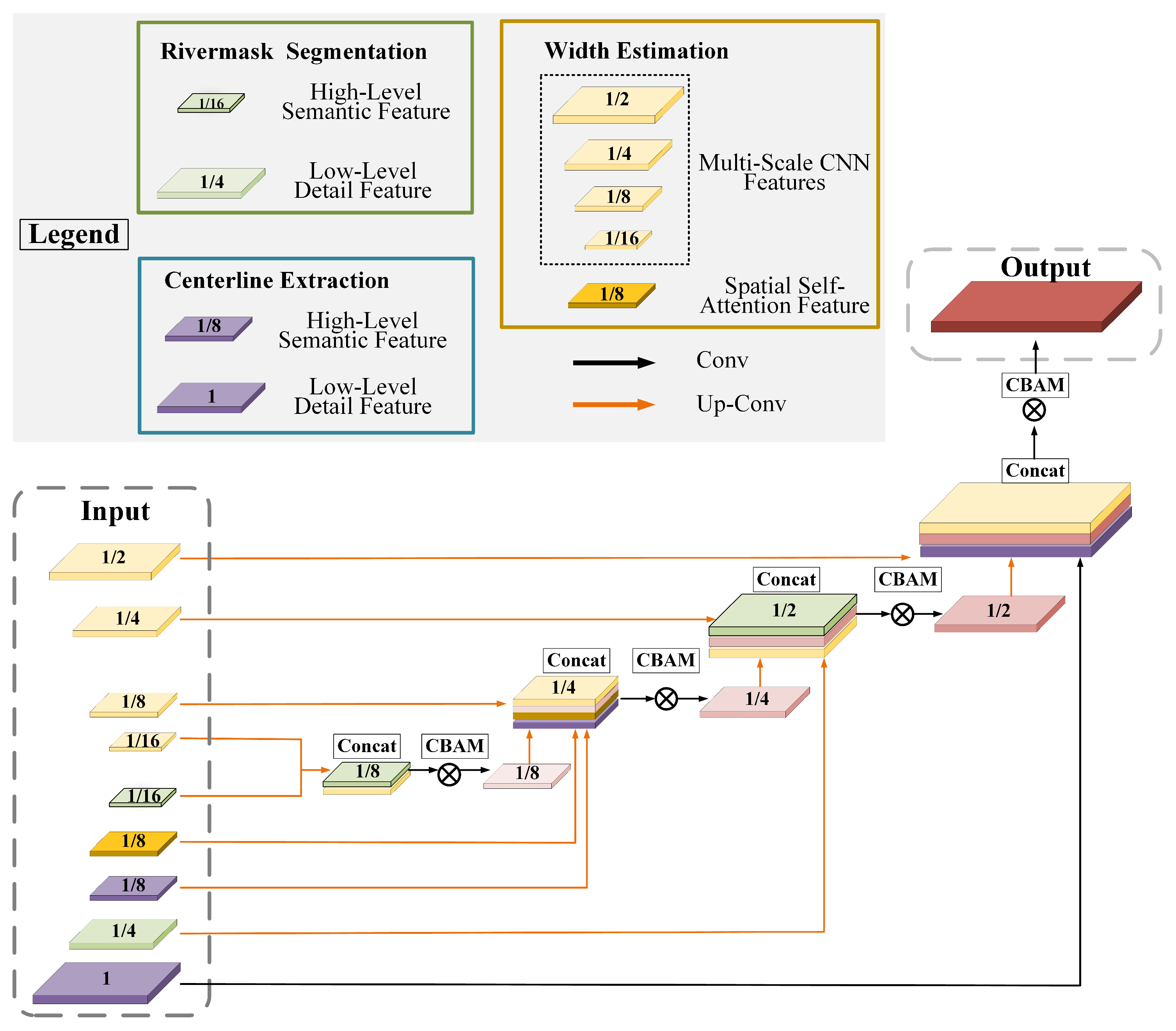
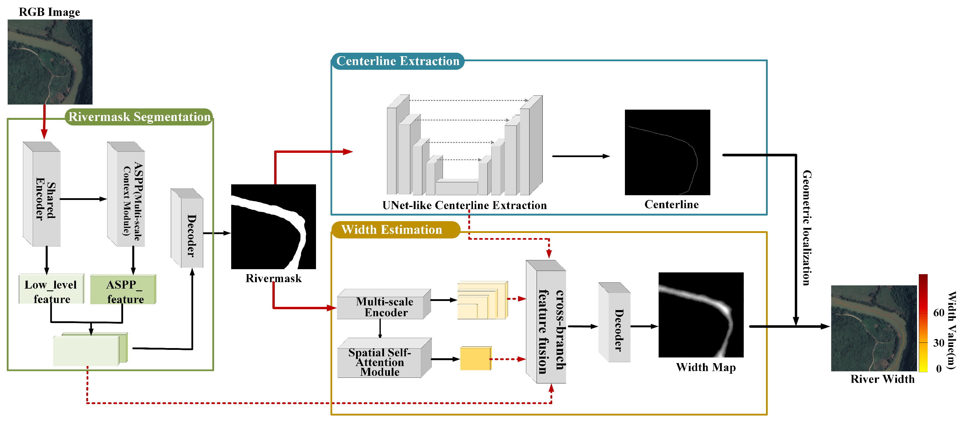
Overview of the proposed E2E-SGRWNet architecture. The network takes high-resolution optical remote sensing imagery as input and adopts a stage-guided multi-task framework composed of river-mask segmentation, centerline extraction, and river-width regression, enabling end-to-end river-width estimation.
Figure 1.
Overview of the proposed E2E-SGRWNet architecture. The network takes high-resolution optical remote sensing imagery as input and adopts a stage-guided multi-task framework composed of river-mask segmentation, centerline extraction, and river-width regression, enabling end-to-end river-width estimation.
Figure 2.
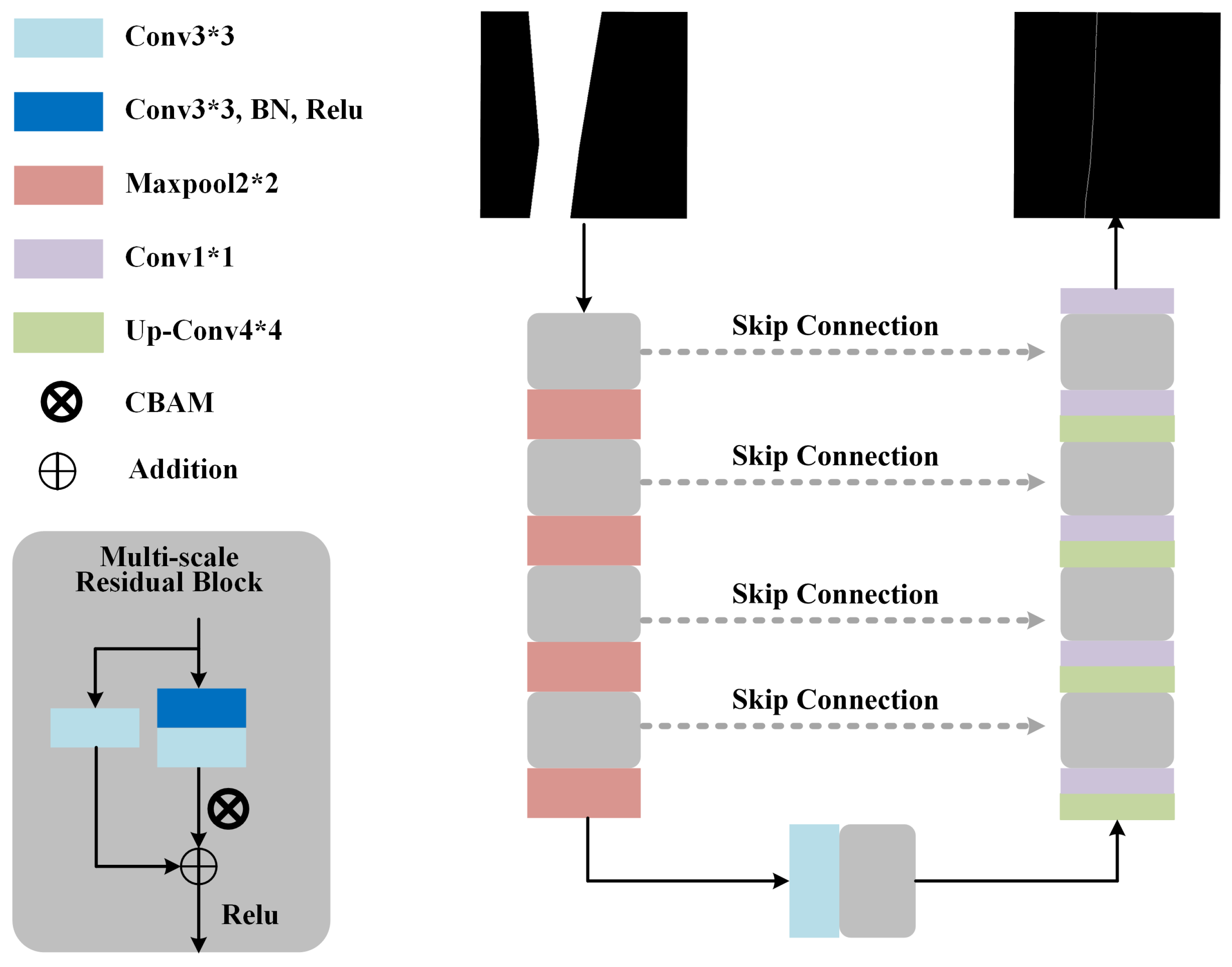
Detailed architecture of the structure-oriented river centerline extraction task. The network follows a U-Net-style encoder–decoder paradigm built upon multi-scale residual convolutional blocks and integrates complementary feature representations across different semantic levels through skip connections between corresponding encoder and decoder stages.
Figure 2.
Detailed architecture of the structure-oriented river centerline extraction task. The network follows a U-Net-style encoder–decoder paradigm built upon multi-scale residual convolutional blocks and integrates complementary feature representations across different semantic levels through skip connections between corresponding encoder and decoder stages.
Figure 3.
Architecture of the cross-branch feature fusion module. This module progressively integrates spatial semantic features from the river-mask segmentation branch and structural features from the river centerline extraction branch, using the multi-scale features and the spatial attention feature from the river-width regression branch as the backbone, thereby enabling collaborative modeling of multi-branch features.
Figure 3.
Architecture of the cross-branch feature fusion module. This module progressively integrates spatial semantic features from the river-mask segmentation branch and structural features from the river centerline extraction branch, using the multi-scale features and the spatial attention feature from the river-width regression branch as the backbone, thereby enabling collaborative modeling of multi-branch features.
Figure 4.
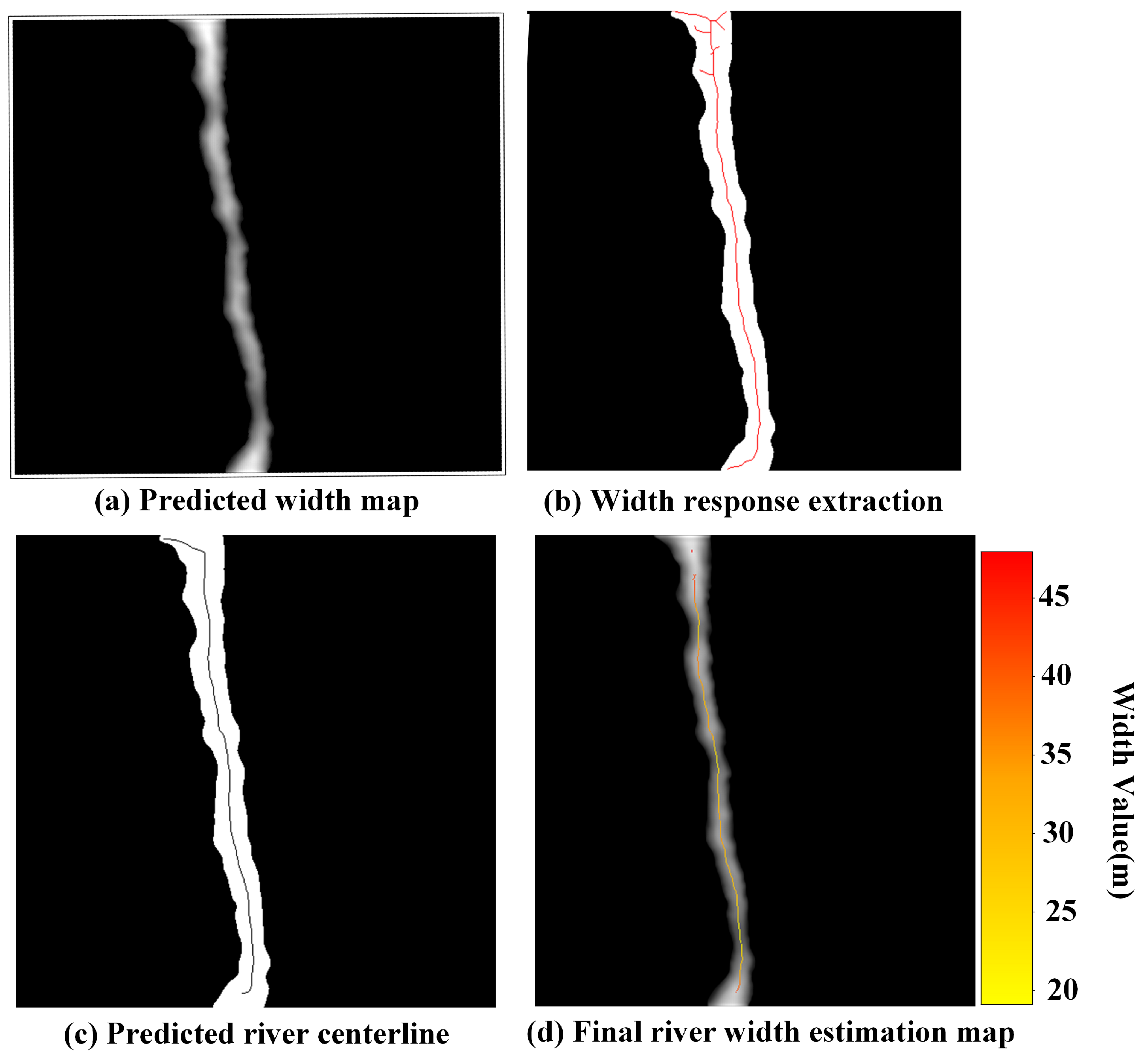
River-width extraction from width-response distribution with structural constraints. (a) Predicted river-width map produced by the width-regression branch; (b) Initial response ridges extracted from the width-response distribution. (c) Predicted river centerline overlaid on the river mask, where black pixels within the river region indicate the centerline locations. (d) Final river-width results extracted from width-response distribution with structural constraints.
Figure 4.
River-width extraction from width-response distribution with structural constraints. (a) Predicted river-width map produced by the width-regression branch; (b) Initial response ridges extracted from the width-response distribution. (c) Predicted river centerline overlaid on the river mask, where black pixels within the river region indicate the centerline locations. (d) Final river-width results extracted from width-response distribution with structural constraints.
Figure 5.
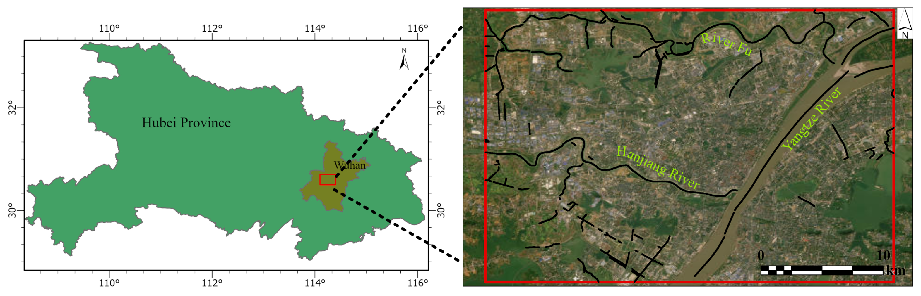
Overview of the Wuhan study area.
Figure 5.
Overview of the Wuhan study area.
Figure 6.
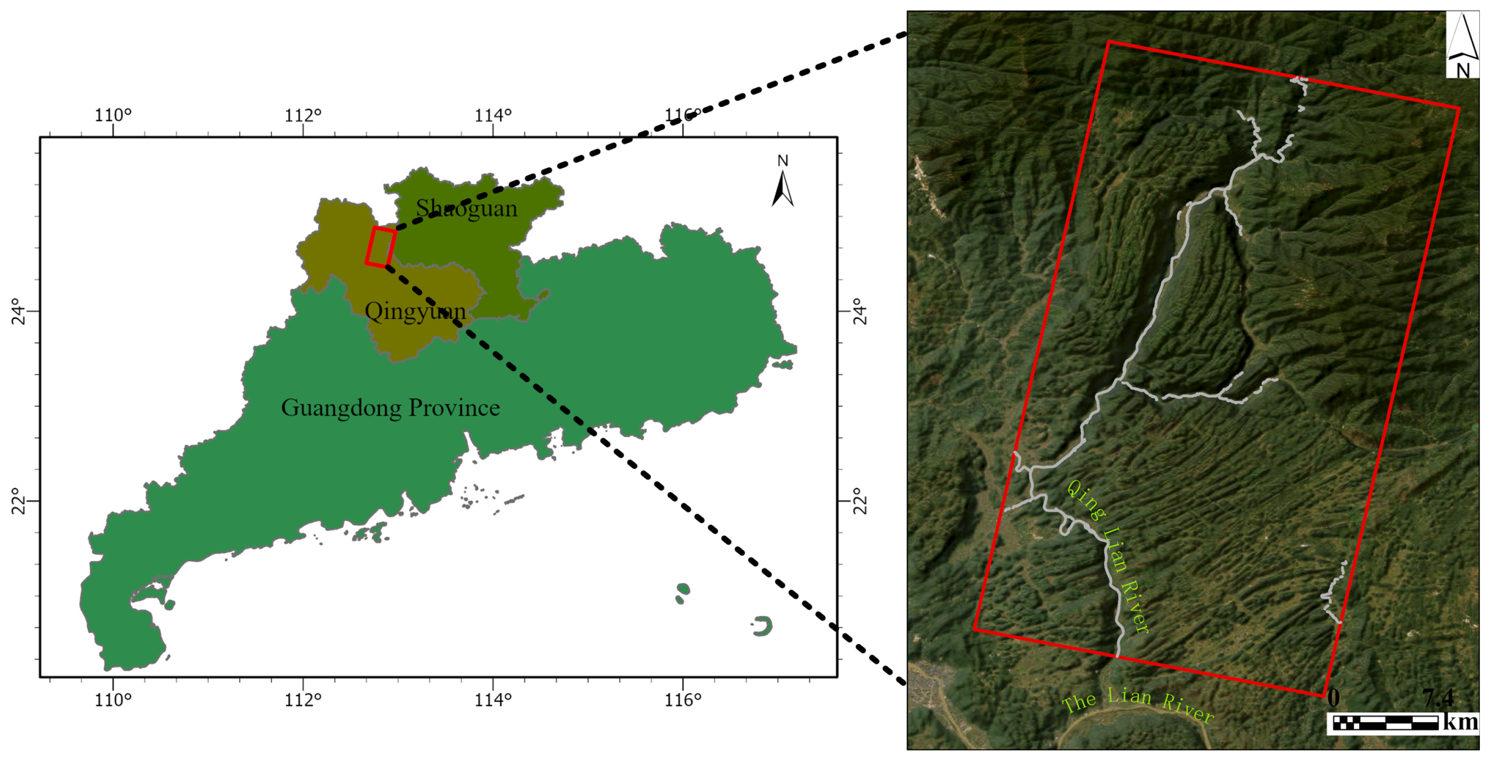
Overview of the Qingyuan study area.
Figure 6.
Overview of the Qingyuan study area.
Figure 7.
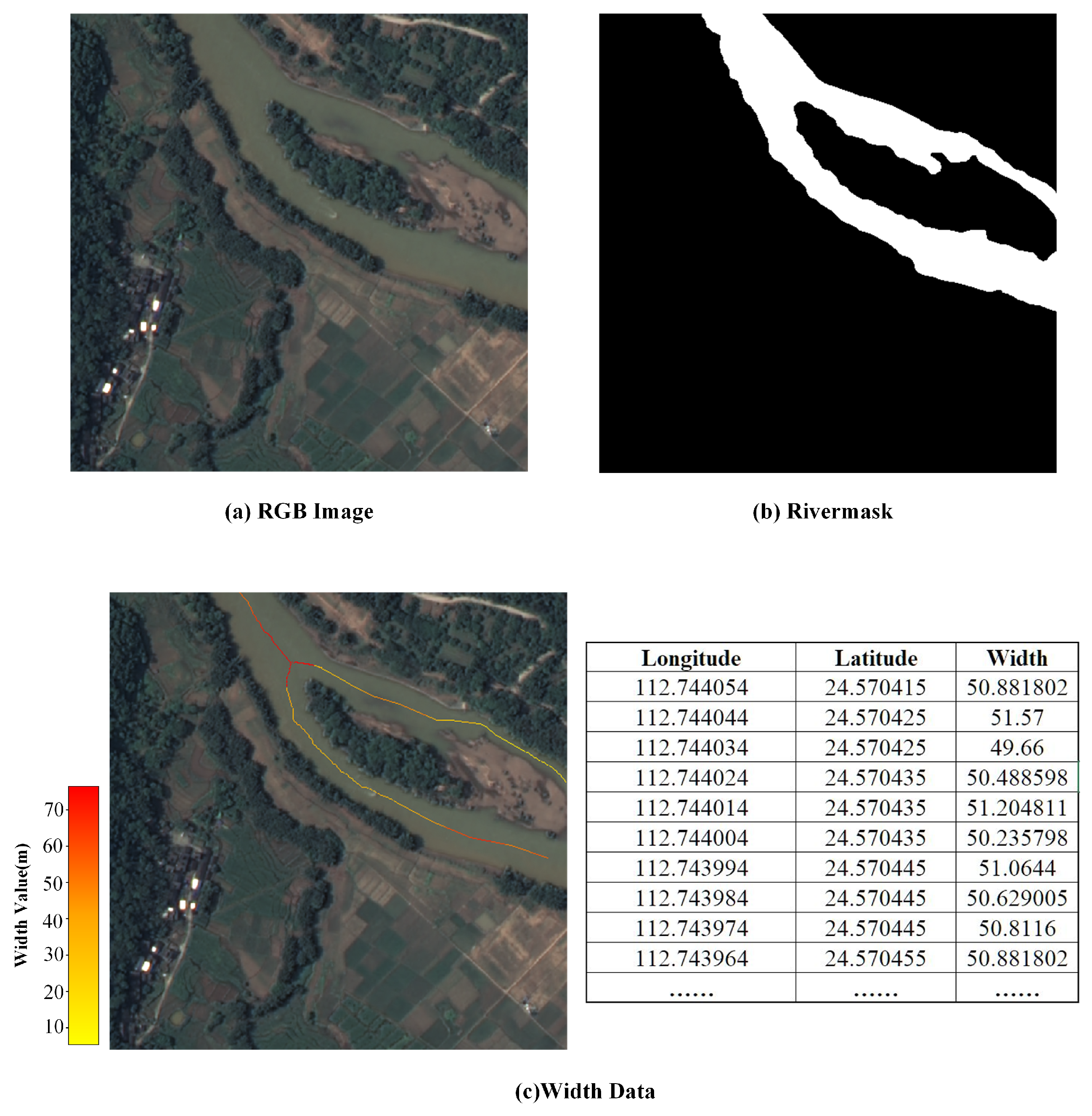
Schematic illustration of the data organization for a river-width sample unit. (a) resolution GF-2 optical remote sensing imagery; (b) the corresponding river-mask; (c) river-width annotations referenced to the centerline for the corresponding river segment.
Figure 7.
Schematic illustration of the data organization for a river-width sample unit. (a) resolution GF-2 optical remote sensing imagery; (b) the corresponding river-mask; (c) river-width annotations referenced to the centerline for the corresponding river segment.
Figure 8.
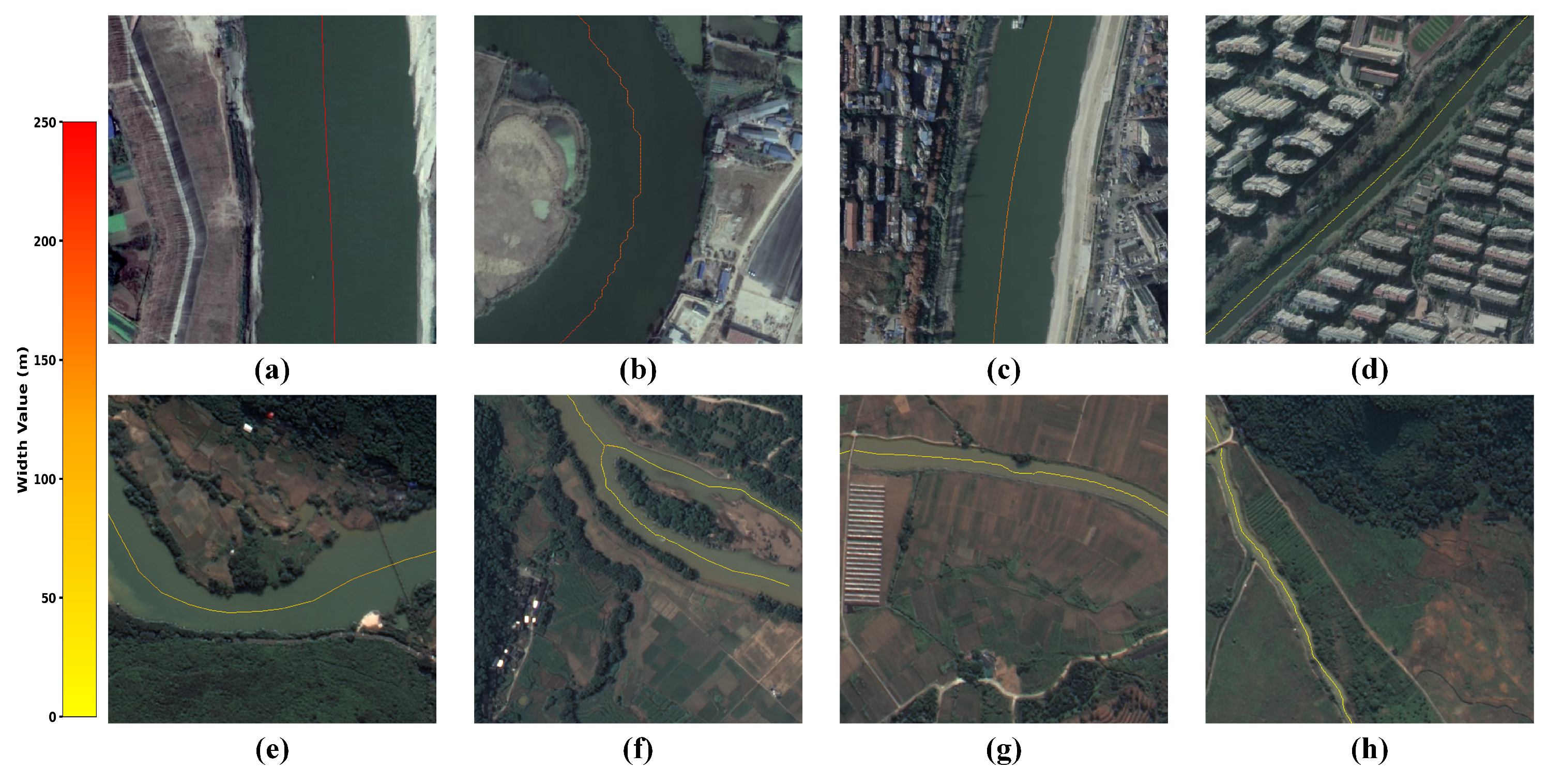
Representative samples from the RiverWidth-HR Dataset. River-width information is overlaid on GF-2 optical remote sensing imagery, covering diverse geographic settings, multiple river-width scales, and a wide range of river morphologies. (a) A wide-river scene with relatively regular riverbanks; (b) a wide-river scene with pronounced channel meandering; (c) a wide-river scene located in an urban built-up area with dense surrounding buildings; (d) a small-river scene in a high-density urban built-up area; (e) a natural wide-river scene with strong background vegetation coverage; (f) a natural medium-width river with multiple branches and complex channel structures; (g) a natural medium-width river in an agricultural landscape with relatively homogeneous surrounding land cover; (h) a natural small-river scene with narrow channel width and evident surrounding vegetation.
Figure 8.
Representative samples from the RiverWidth-HR Dataset. River-width information is overlaid on GF-2 optical remote sensing imagery, covering diverse geographic settings, multiple river-width scales, and a wide range of river morphologies. (a) A wide-river scene with relatively regular riverbanks; (b) a wide-river scene with pronounced channel meandering; (c) a wide-river scene located in an urban built-up area with dense surrounding buildings; (d) a small-river scene in a high-density urban built-up area; (e) a natural wide-river scene with strong background vegetation coverage; (f) a natural medium-width river with multiple branches and complex channel structures; (g) a natural medium-width river in an agricultural landscape with relatively homogeneous surrounding land cover; (h) a natural small-river scene with narrow channel width and evident surrounding vegetation.
Figure 9.
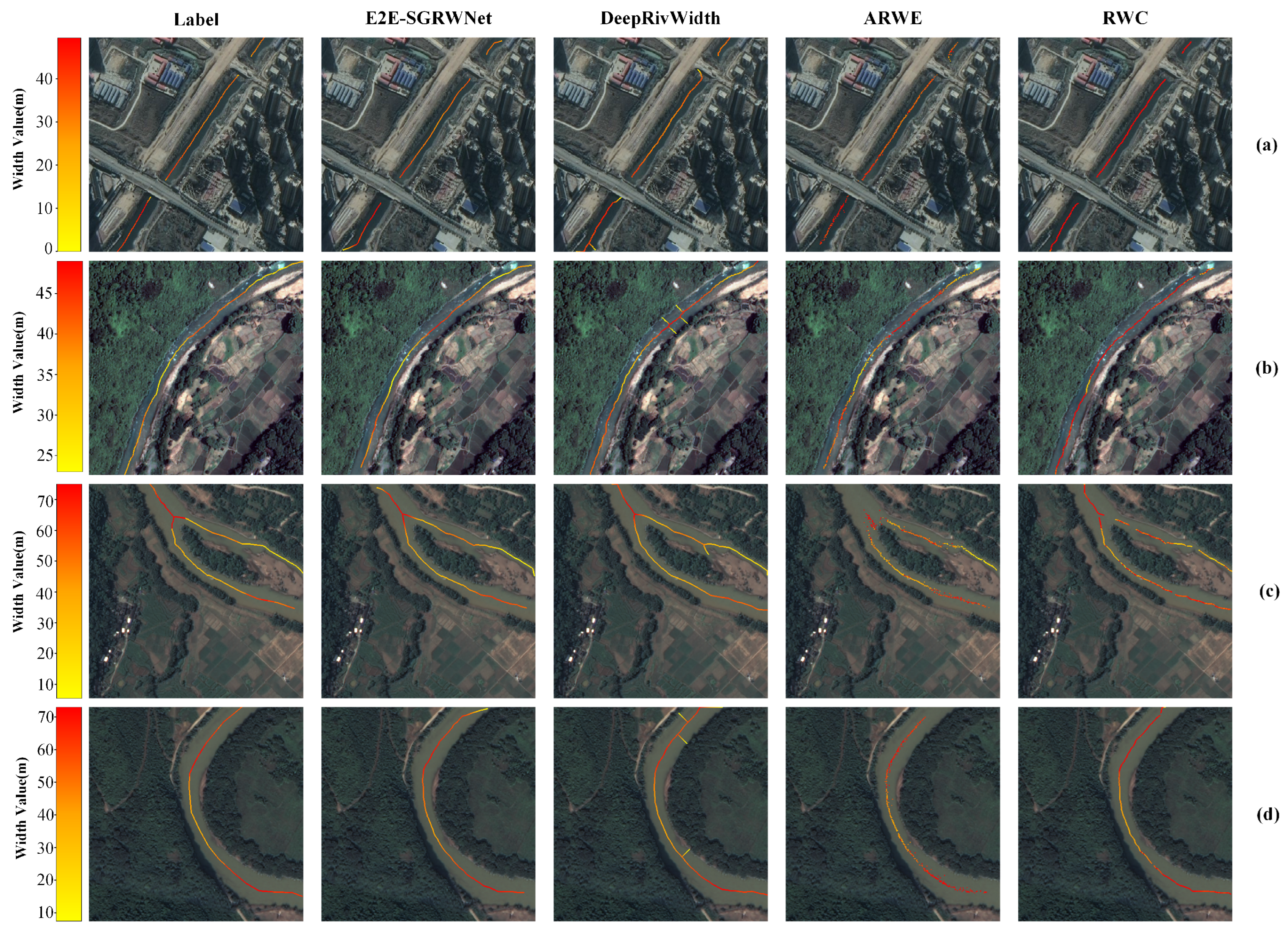
Qualitative comparison of river-width estimation results in representative scenes from the high-precision river-width dataset. (a) A typical urban scene; (b–d) representative natural scenes. The examples cover different river-width classes and diverse channel morphologies. For each scene, the ground-truth width annotations and the results produced by the four methods are shown in sequence. Each scene is equipped with an independent color legend that maps river-width values to corresponding colors.
Figure 9.
Qualitative comparison of river-width estimation results in representative scenes from the high-precision river-width dataset. (a) A typical urban scene; (b–d) representative natural scenes. The examples cover different river-width classes and diverse channel morphologies. For each scene, the ground-truth width annotations and the results produced by the four methods are shown in sequence. Each scene is equipped with an independent color legend that maps river-width values to corresponding colors.
Figure 10.
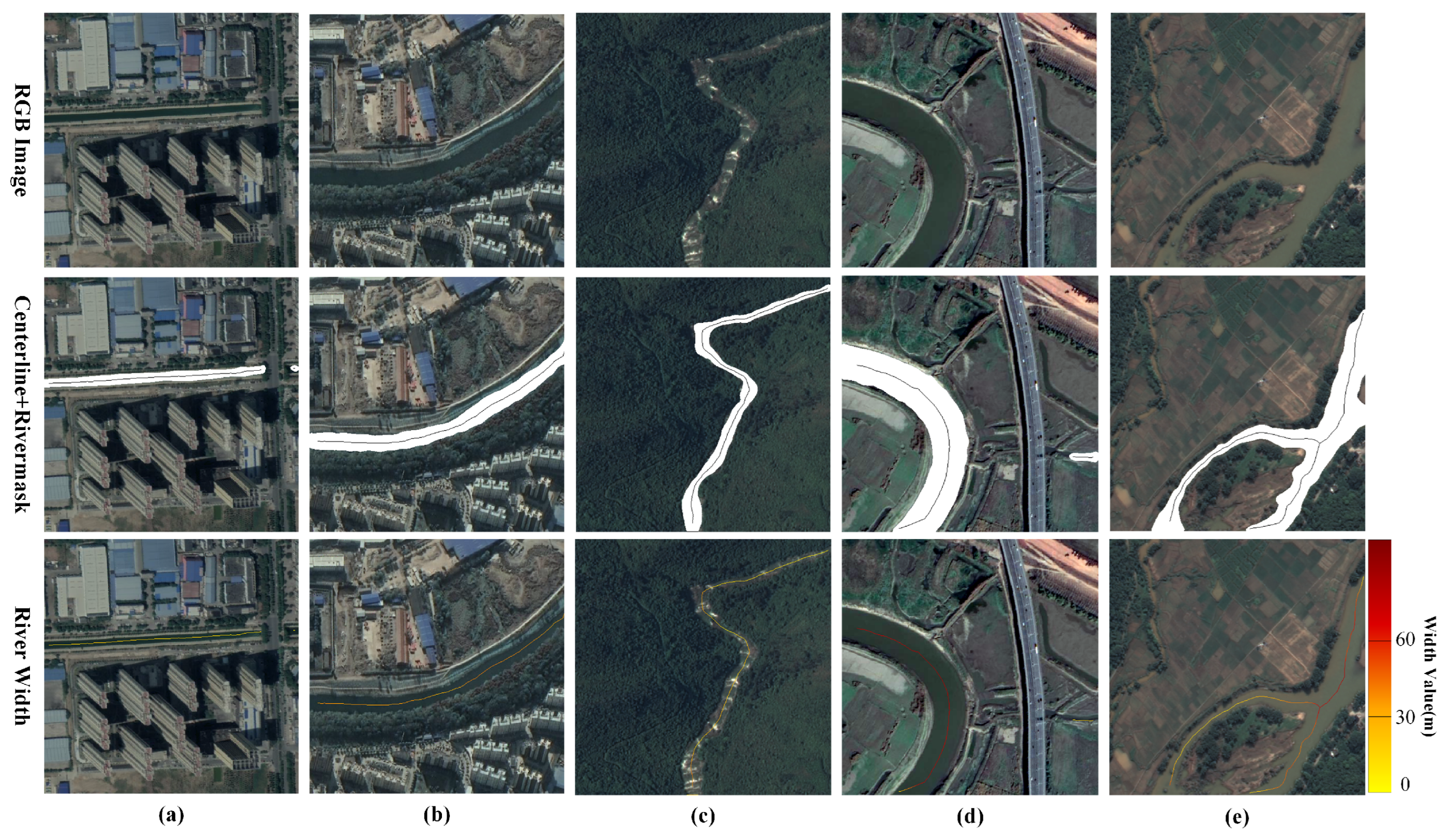
Qualitative analysis results. Five representative river samples are selected from the test set for segmentation and width estimation. The first row shows the corresponding resolution GF-2 optical remote sensing imagery. The second row visualizes the river-mask segmentation and centerline segmentation results overlaid on the imagery, where white regions denote river areas and black pixels indicate centerline locations. The third row presents the river-width prediction results overlaid on the original imagery, where width values are mapped to colors according to a shared color legend. (a) An urban scene with a narrow river channel surrounded by dense buildings; (b) An urban scene with a medium-width river channel within a densely built environment; (c) A mountainous scene featuring a narrow stream with extensive forest vegetation; (d) A natural river reach exhibiting abrupt changes in flow direction; (e) An agricultural landscape with a highly branched river network and complex channel morphology.
Figure 10.
Qualitative analysis results. Five representative river samples are selected from the test set for segmentation and width estimation. The first row shows the corresponding resolution GF-2 optical remote sensing imagery. The second row visualizes the river-mask segmentation and centerline segmentation results overlaid on the imagery, where white regions denote river areas and black pixels indicate centerline locations. The third row presents the river-width prediction results overlaid on the original imagery, where width values are mapped to colors according to a shared color legend. (a) An urban scene with a narrow river channel surrounded by dense buildings; (b) An urban scene with a medium-width river channel within a densely built environment; (c) A mountainous scene featuring a narrow stream with extensive forest vegetation; (d) A natural river reach exhibiting abrupt changes in flow direction; (e) An agricultural landscape with a highly branched river network and complex channel morphology.

Figure 11.
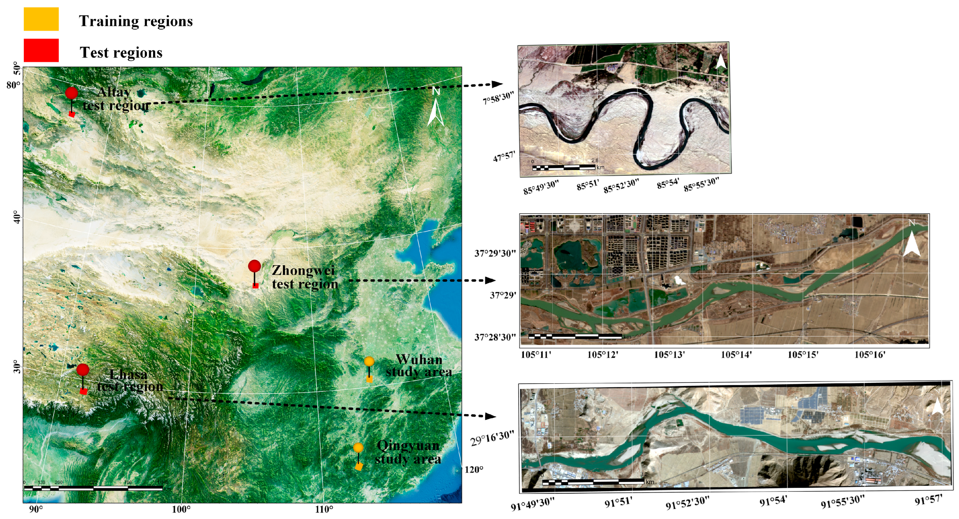
Locations of the training regions and cross-region test sites. Yellow boxes indicate the training regions used to construct the RiverWidth-HR dataset and train the E2E-SGRWNet, while red boxes represent the cross-region test sites.
Figure 11.
Locations of the training regions and cross-region test sites. Yellow boxes indicate the training regions used to construct the RiverWidth-HR dataset and train the E2E-SGRWNet, while red boxes represent the cross-region test sites.
Figure 12.
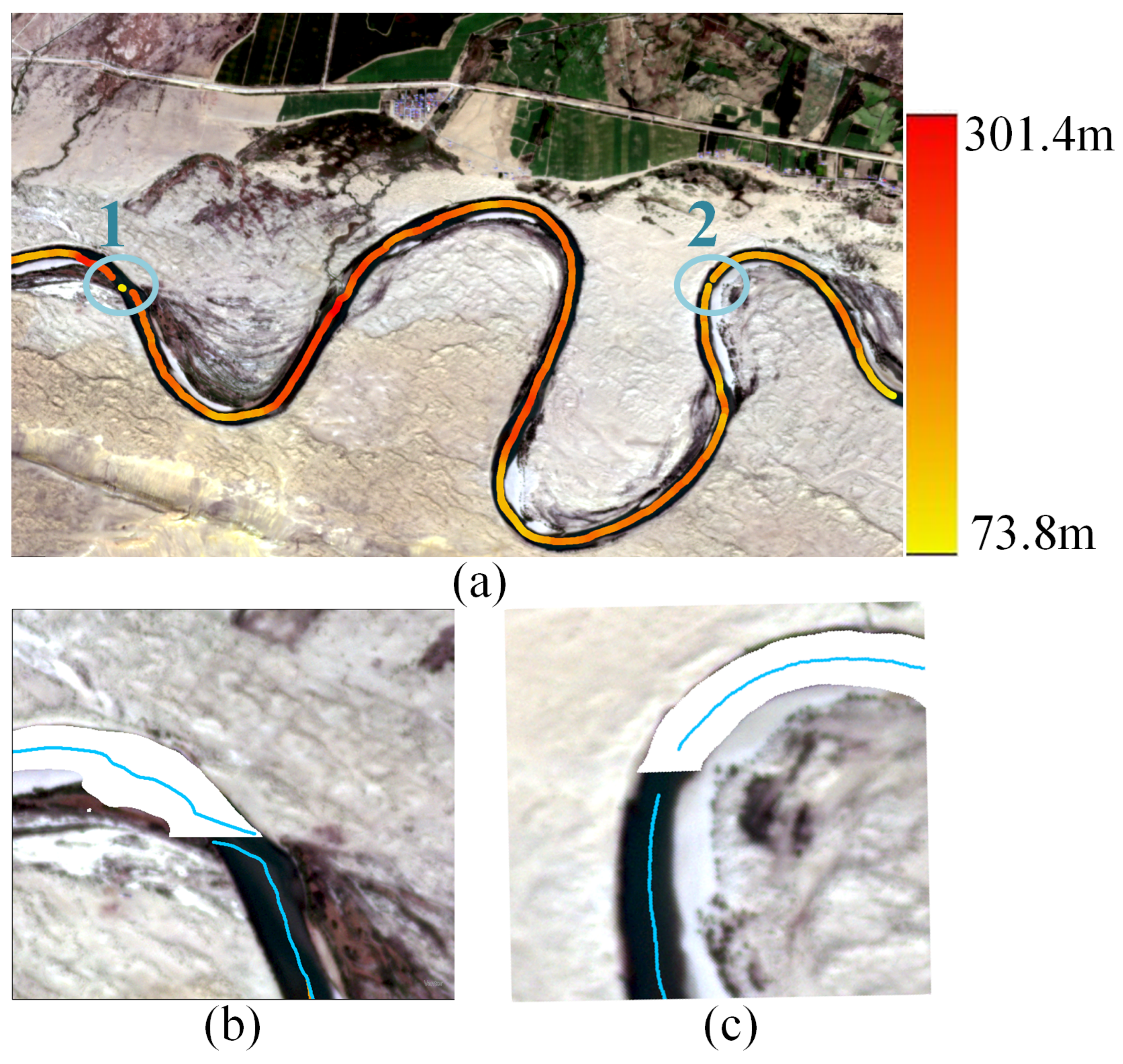
River-width prediction results of E2E-SGRWNet in the Altay test region. (a) Overall river-width classification results for the test area, where the marked points 1 and 2 indicate two typical locations with prediction errors. (b,c) Local details corresponding to points 1 and 2 in (a), respectively. White pixels represent the river-mask segmentation results, and blue pixels indicate the predicted river centerlines. To illustrate the boundary between adjacent image tiles, only the river-mask results from the upper tile are displayed within the local region, while the adjacent tile retains only the centerline results.
Figure 12.
River-width prediction results of E2E-SGRWNet in the Altay test region. (a) Overall river-width classification results for the test area, where the marked points 1 and 2 indicate two typical locations with prediction errors. (b,c) Local details corresponding to points 1 and 2 in (a), respectively. White pixels represent the river-mask segmentation results, and blue pixels indicate the predicted river centerlines. To illustrate the boundary between adjacent image tiles, only the river-mask results from the upper tile are displayed within the local region, while the adjacent tile retains only the centerline results.
Figure 13.
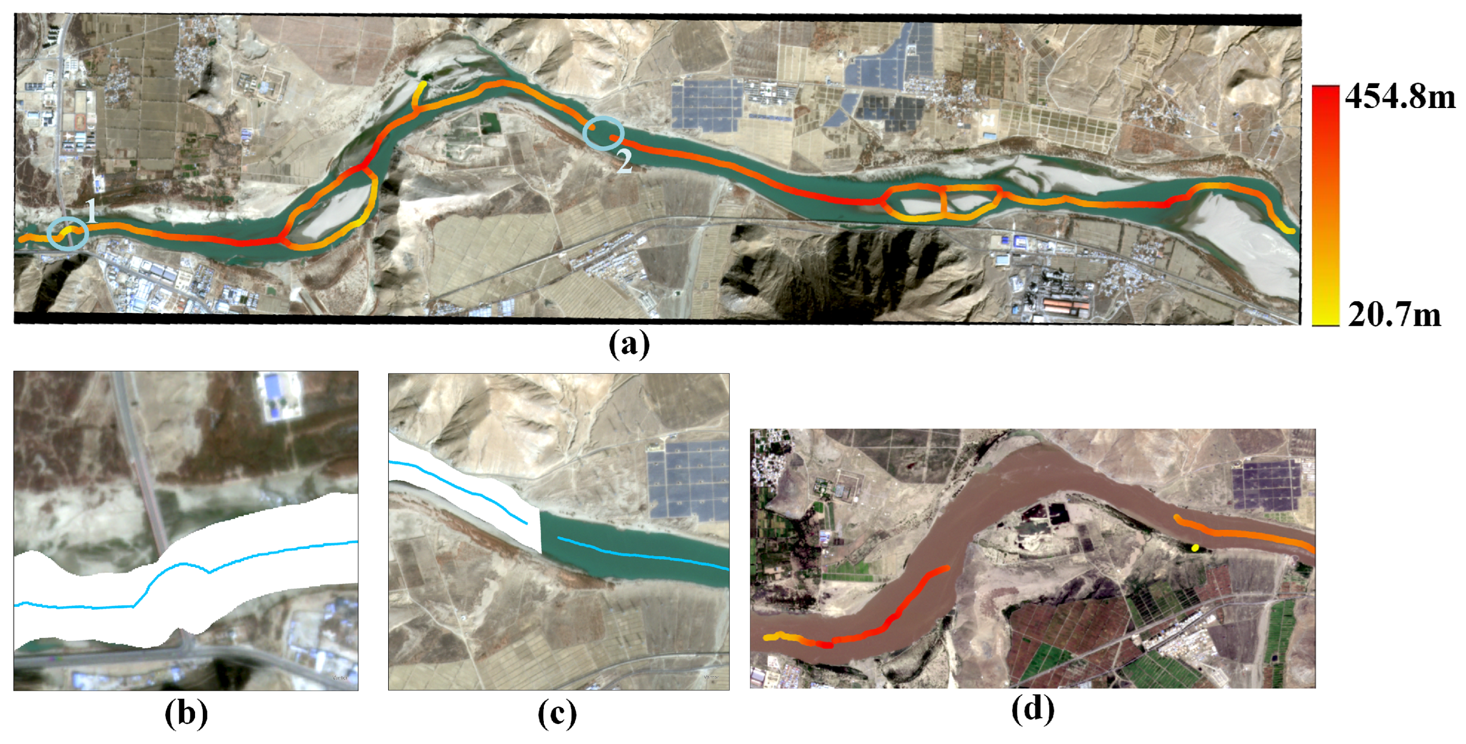
River-width prediction results of E2E-SGRWNet in the Lhasa test region. (a) Overall river-width classification results for the test area, where the marked points 1 and 2 indicate two typical locations with prediction errors. (b,c) Local details corresponding to points 1 and 2 in (a), respectively. White pixels represent the predicted river-mask results, and blue pixels indicate the predicted river centerlines. In (c), to illustrate the boundary between adjacent image tiles, only the river-mask results from the left tile are displayed within the local region, while the adjacent tile retains only the centerline results. (d) River-width prediction results for a local area of the test region imagery under summer conditions.
Figure 13.
River-width prediction results of E2E-SGRWNet in the Lhasa test region. (a) Overall river-width classification results for the test area, where the marked points 1 and 2 indicate two typical locations with prediction errors. (b,c) Local details corresponding to points 1 and 2 in (a), respectively. White pixels represent the predicted river-mask results, and blue pixels indicate the predicted river centerlines. In (c), to illustrate the boundary between adjacent image tiles, only the river-mask results from the left tile are displayed within the local region, while the adjacent tile retains only the centerline results. (d) River-width prediction results for a local area of the test region imagery under summer conditions.
Figure 14.
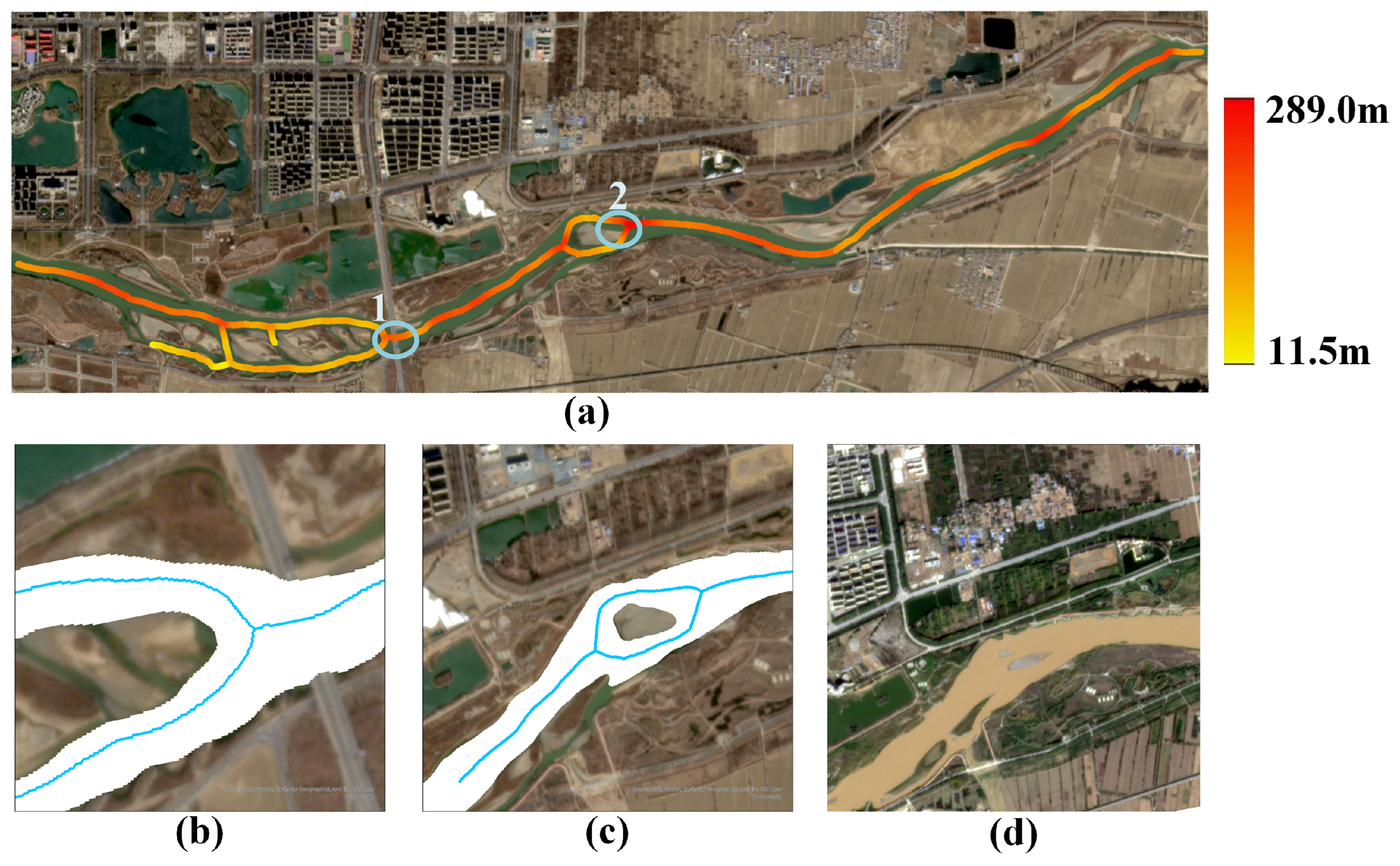
River-width prediction results of E2E-SGRWNet in the Zhongwei test region. (a) Overall river-width classification results for the test area, where the marked points 1 and 2 indicate two typical locations with prediction errors. (b,c) Local details corresponding to points 1 and 2 in (a), respectively. White pixels represent the predicted river-mask results, and blue pixels indicate the predicted river centerlines. (d) Original remote sensing imagery of a local area in the test region under summer conditions.
Figure 14.
River-width prediction results of E2E-SGRWNet in the Zhongwei test region. (a) Overall river-width classification results for the test area, where the marked points 1 and 2 indicate two typical locations with prediction errors. (b,c) Local details corresponding to points 1 and 2 in (a), respectively. White pixels represent the predicted river-mask results, and blue pixels indicate the predicted river centerlines. (d) Original remote sensing imagery of a local area in the test region under summer conditions.
Table 1.
Distribution of river-width classes in the study areas.
Table 1.
Distribution of river-width classes in the study areas.
| River Class | Width Range (m) | Total Length (km) |
|---|
| Wuhan Study Area | Qingyuan Study Area |
|---|
| Small | <30 | 27.38 | 35.77 |
| Medium | 30–60 | 28.83 | 26.46 |
| Large | >60 | 77.78 | 18.55 |
Table 2.
Quantitative evaluation results of river-width estimation for different methods on the test set.
Table 2.
Quantitative evaluation results of river-width estimation for different methods on the test set.
| Method | MAE ↓ | RMSE ↓ | MRE ↓ | PPUR ↑ | GTCR ↑ |
|---|
| RWC | 24.800 | 61.842 | 74.0% | 67.6% | 80.9% |
| ARWE | 5.700 | 18.272 | 19.2% | 64.3% | 80.8% |
| DeepRivWidth | 3.466 | 4.536 | 15.6% | 56.9% | 85.9% |
| E2E-SGRWNet | 3.428 | 4.362 | 13.6% | 61.8% | 80.3% |
Table 3.
Width prediction errors across different river-width categories in the test set (small: <30 m; medium-sized: 30–; large: >60 m).
Table 3.
Width prediction errors across different river-width categories in the test set (small: <30 m; medium-sized: 30–; large: >60 m).
| Method | MAE ↓ | RMSE ↓ | MRE ↓ |
|---|
| Small | Medium | Large | Small | Medium | Large | Small | Medium | Large |
|---|
| RWC | 13.483 | 30.716 | 45.194 | 36.979 | 71.597 | 88.771 | 75.5% | 69.9% | 63.3% |
| ARWE | 4.806 | 7.143 | 10.991 | 14.540 | 22.439 | 26.692 | 35.3% | 16.9% | 15.8% |
| DeepRivWidth | 2.805 | 3.520 | 6.217 | 4.041 | 5.212 | 8.688 | 25.3% | 8.0% | 8.7% |
| E2E-SGRWNet | 3.143 | 3.225 | 5.076 | 4.053 | 4.353 | 6.890 | 19.8% | 7.5% | 7.3% |
Table 4.
Width prediction errors for subdivided river-width intervals (<30 m) in the test set.
Table 4.
Width prediction errors for subdivided river-width intervals (<30 m) in the test set.
| Method | MAE ↓ | RMSE ↓ | MRE ↓ |
|---|
| <10 m | 10–20 m | 20–30 m | <10 m | 10–20 m | 20–30 m | <10 m | 10–20 m | 20–30 m |
|---|
| RWC | 5.946 | 11.486 | 14.583 | 16.039 | 32.039 | 39.780 | 104.5% | 69.9% | 61.8% |
| ARWE | 5.818 | 4.608 | 4.810 | 11.153 | 13.812 | 15.604 | 90.5% | 30.5% | 20.0% |
| DeepRivWidth | 3.430 | 2.570 | 2.634 | 4.723 | 3.884 | 3.893 | 68.3% | 17.2% | 11.1% |
| E2E-SGRWNet | 3.065 | 2.687 | 3.531 | 4.153 | 3.504 | 4.434 | 43.4% | 17.7% | 15.1% |
Table 5.
Evaluation of river-mask segmentation maps and centerline segmentation maps on the test set at spatial resolution. All metrics are computed only over foreground pixels.
Table 5.
Evaluation of river-mask segmentation maps and centerline segmentation maps on the test set at spatial resolution. All metrics are computed only over foreground pixels.
| Task | IoU | Precision | Recall | F1 |
|---|
| River mask | 0.908 | 0.983 | 0.922 | 0.952 |
| River centerline | 0.519 | 0.687 | 0.680 | 0.684 |
Table 6.
River-width prediction errors for the three test regions. All results were obtained from resolution PlanetScope imagery.
Table 6.
River-width prediction errors for the three test regions. All results were obtained from resolution PlanetScope imagery.
| Region | MAE (m) | RMSE (m) | MRE |
|---|
| Altay | | | |
| Lhasa | | | |
| Zhongwei | | | |
Table 7.
Ablation results of E2E-SGRWNet under different stage-wise guidance configurations on the spatial resolution test set.
Table 7.
Ablation results of E2E-SGRWNet under different stage-wise guidance configurations on the spatial resolution test set.
| Model | MAE ↓ | RMSE ↓ | MRE ↓ | PPUR ↑ | GTCR ↑ |
|---|
| Model_1 | 9.830 | 12.196 | 29.2% | 37.8% | 54.1% |
| Model_2 | 3.897 | 5.114 | 15.8% | 61.2% | 79.0% |
| Model_3 | 3.396 | 4.582 | 13.4% | 58.5% | 78.5% |
| E2E-SGRWNet | 3.428 | 4.362 | 13.6% | 61.8% | 80.3% |