Article

A Deformable Dual-Branch Visual State-Space Network for Landslide Identification with Multi-Scale Recognition and Irregular Boundary Enhancement

1
School of Transportation Science and Engineering, Beihang University, Beijing 100191, China
2
China Institute of Geo-Environment Monitoring (Guide Center of Prevention Technology for Geo-Hazards, MNR), Beijing 100081, China
*
Author to whom correspondence should be addressed.
Remote Sens. 2026, 18(5), 707; https://doi.org/10.3390/rs18050707
Submission received: 28 January 2026 / Revised: 22 February 2026 / Accepted: 25 February 2026 / Published: 27 February 2026

Highlights

What are the main findings?
  • A deformable dual-branch visual state-space network (DFmamba) effectively improves landslide segmentation accuracy.
  • The proposed architecture shows strong robustness across multi-scale, complex-boundary, and cross-domain scenarios, significantly reducing boundary fragmentation, missed detections of large landslide bodies, and detail loss in small-scale landslides.
What are the implications of the main findings?
  • This study demonstrates that selective state-space modeling combined with deformable boundary refinement is a practical solution for large-area, high-resolution landslide mapping, enabling globally consistent interpretation without the heavy computational cost of attention-based models.
  • DFmamba provides a transferable and deployable framework for operational landslide monitoring and emergency response, supporting reliable delineation of landslide extents under varying geomorphological conditions and imaging domains.

Abstract

In recent years, rapid and reliable interpretation for emergency response to landslides and other geological hazards has become increasingly important. This paper presents DFmamba, an improved deformable dual-branch visual state-space network, to address engineering challenges such as missed large landslide bodies, boundary shifts, and loss of small-scale details. DFmamba mitigates the limited effective receptive field and window-partition constraints that often prevent existing methods from balancing large-area semantic consistency, multi-scale detection, precise boundary delineation, and computational efficiency. It employs a parallel encoder with a convolutional branch and a Visual State-Space Model (VSSM) branch to jointly capture local textures and global context. In the decoder, deformable residual blocks (DRB) enhance geometric modeling of irregular boundaries, while multi-scale feature alignment and a shallow high-frequency injection (MFP) mechanism strengthen boundary responses and preserve fine details. Experiments on the public CAS dataset against representative CNN-, Transformer-, and SSM-based baselines show that DFmamba achieves improved Precision, Recall, F1-score, and IoU, with stable performance across multi-scale scenarios, demonstrating strong robustness for landslide segmentation.

1. Introduction

Landslides occur frequently worldwide and rank among the most common geological hazards [1]. They not only inflict severe damage on regional ecosystems and infrastructure but also often trigger secondary disasters such as flash floods and debris flows [2], leading to significant casualties and economic losses and, in some cases, catastrophic consequences [3]. Consequently, rapid and accurate landslide identification and mapping have become key issues in disaster prevention and risk assessment [4]. Remote-sensing monitoring of landslide-prone areas and the establishment of landslide inventories are essential components for building landslide identification, monitoring, and early warning systems, forming the foundation of proactive disaster mitigation [5].
In recent years, deep learning has gradually become the mainstream technical route for landslide identification and segmentation [6]. In this work, we focus on pixel-level landslide segmentation from high-resolution optical remote-sensing imagery, where a model predicts a binary mask that delineates landslide regions for a given large-scene image. In practical post-disaster mapping, images often span broad areas with dense pixels, so training and inference commonly rely on tiled or sliding-window processing. This setting simultaneously requires (i) cross-tile semantic consistency for large landslide bodies and (ii) fine-grained delineation for small landslides and irregular boundaries under strong background interference [4]. The existing approaches can be broadly categorized into two types: (i) pixel-wise classification or encoder–decoder frameworks based on convolutional neural networks (CNNs) [7], such as U-Net and its variants, which are effective at capturing local textures and boundary cues; and (ii) Transformer frameworks that introduce self-attention to model long-range dependencies over larger contexts, thereby enhancing semantic representation [8]. Despite their respective advantages, both face limitations in landslide mapping scenarios [9]. CNNs have limited effective receptive fields and often rely on patch-wise convolutions, dilated convolutions, or pyramid-style local aggregation to enlarge the apparent receptive field [10] yet may still struggle to maintain continuous and consistent semantic representations beyond local neighborhoods [11]. Transformers typically depend on patching or windowed modeling, where cross-window interactions are restricted and computational costs are substantial [12]. Various CNN + Transformer hybrids attempt to strike a balance between local and global modeling [13], but in real-world large-scene applications, they may still exhibit insufficient global context utilization, reduced efficiency, and unstable fine-detail depiction during multi-scale fusion and decoding [14].
Comprehensive landslide segmentation under the setting described above remains challenging and reveals several gaps that are insufficiently addressed in existing pipelines [14]. First, pronounced scale variation: small landslides and large expansive ones often coexist within the same area, leading to wide differences in spatial extent [12]. When confronted with large instances under tiled processing, the existing methods may produce globally incoherent semantics, incomplete coverage, or fragmented masks [15,16]. Second, complex boundaries and shapes: landslide margins are often jagged, tortuous, branched, and irregular, with fragmented blocks coexisting alongside elongated tongue-like structures [17]. Convolution kernels with fixed sampling positions or patches of fixed size are not always adequate to adaptively align with such geometric variation [15], which can intensify contour mismatches and errors near boundaries [18]. Third, loss of low-level details: low-level features carry rich textures and high-frequency cues, such as fissures on rock–soil surfaces, slip traces, and fine collapse edges, that are crucial for identifying small-scale landslides and transitional boundary zones [19]. Yet current pipelines, during multi-scale fusion and upsampling, tend to emphasize high-level semantics [20]; shallow details may be weakened or averaged out and thus contribute less to the final decision, degrading small-object recall and boundary precision [21]. Fourth, whole-image scale and operational constraints: high-resolution scenes contain a large number of pixels and strong background interference, imposing significant computational and memory burdens for training and inference [4]. Models must balance accuracy with throughput and latency to meet the timeliness requirements of batch mapping and emergency applications [22].
Recently, Selective State Space Models (Selective SSMs), exemplified by Mamba, have opened new opportunities for global modeling with favorable computational characteristics [23]. Such models establish long-range dependencies via linear-time state updates to sequences and, through content-selection mechanisms, dynamically filter and retain key information during propagation [24]. For vision tasks, two-dimensional images can be serialized (e.g., by rows, columns, or snake-like paths) for selective scanning [25], enabling distant pixels to interact without explicitly constructing dense attention matrices among all tokens [26,27]. This property motivates exploring selective SSMs to mitigate semantic discontinuity across large scenes under tiled processing. However, effectively integrating selective scanning and state recursion into the landslide segmentation paradigm still requires structured designs that jointly account for scale variation, boundary irregularity, detail preservation, and whole-image inference constraints [28,29].
Motivated by the gaps outlined above, we propose DFmamba, a deformable dual-branch visual state-space network for landslide segmentation. DFmamba is designed to jointly model local texture/boundary cues and large-scene semantic propagation within a unified framework, while incorporating boundary-aware refinement and explicit detail-preservation mechanisms to better fit the irregular geometry and multi-scale characteristics of landslides under practical tiled inference.
The main contributions are as follows.
(1)
We design a dual-branch visual state-space framework that enables complementary modeling of local details and global semantic propagation for high-resolution landslide segmentation and supports large-scene semantic consistency under tiled processing.
(2)
We develop a geometry-adaptive refinement mechanism in the decoder to enhance contour alignment for irregular boundaries and slender structures.
(3)
We design an explicit detail-preservation strategy to retain shallow high-frequency cues during multi-scale fusion and upsampling, benefiting small-object and boundary-transition delineation.
Moreover, the proposed framework leverages selective state recursion for global modeling rather than heavyweight global attention, aiming to keep training and inference costs controllable for large-area landslide mapping.

2. Method and Dataset

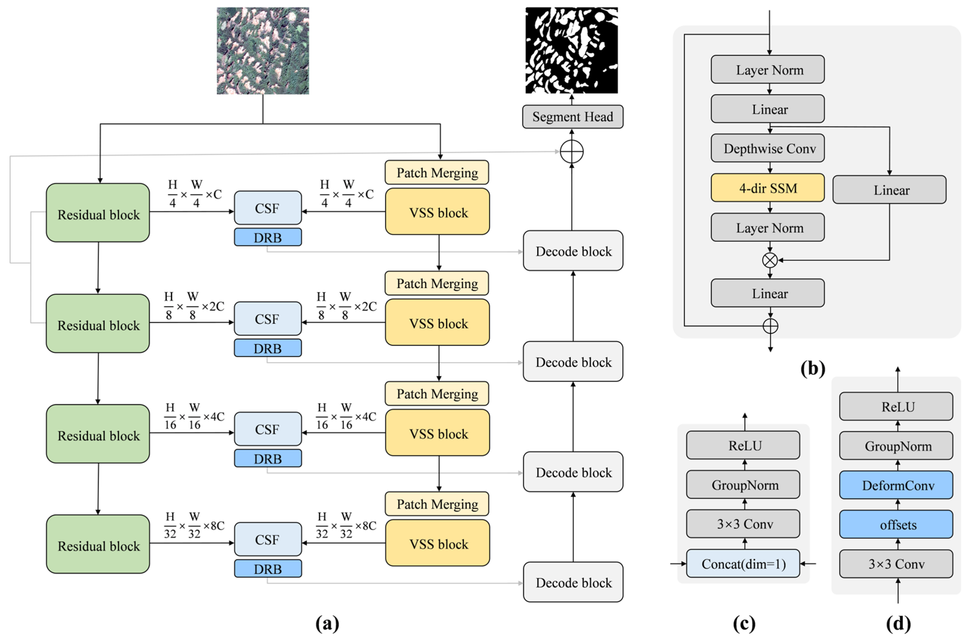
The proposed DFmamba adopts a dual-branch architecture (Figure 1) consisting of a CNN branch built on ResNet-50 and a state-space modeling branch implemented by a VSSMEncoder. The CNN branch is responsible for extracting local textures and boundary cues, while the VSSM branch focuses on propagating global context via selective state-space scanning. To couple local and global representations, DFmamba performs stage-wise cross-branch interaction with cross-scale alignment, where features from the two branches are exchanged and aligned at multiple resolutions. In the decoding stage, we introduce a Deformable Residual Block (DRB) as a boundary-aware refinement module with learnable sampling offsets to adapt to irregular landslide contours. A lightweight U-shaped decoder then progressively restores spatial resolution and produces the final feature maps, and a segmentation head outputs pixel-level landslide masks. Overall, the architecture is designed to jointly support large-scene semantic propagation, multi-scale feature consistency, and boundary-sensitive delineation under tiled high-resolution remote-sensing inference.

2.1. VSSMEncoder

In deep learning, State Space Models (SSMs) have attracted growing attention due to their ability to model long-range dependencies with favorable computational properties [30]. From a continuous time perspective, an SSM maps an input sequence x ( t ) to an output y ( t ) through a linear dynamical system [31]:
h ˙ ( t ) = A h ( t ) + B x ( t )
y ( t ) = C h ( t ) + D x ( t )
where h ˙ ( t ) denotes the hidden state, and A ,   B ,   C ,   a n d   D parameterize state evolution, input projection, output projection, and direct feedthrough, respectively. For efficient computation in neural networks, Equations (1) and (2) are typically discretized (e.g., under the zero-order hold assumption), yielding the recurrent form:
h k = Φ h k 1 + Γ x k
y k = C h k + D x k
where Φ = e A Δ T is the state transition matrix and Γ = ( e A Δ T I ) A 1 B is the input projection matrix. This formulation enables sequence modeling via recursive state updates. Building on this idea, Mamba introduces selective scanning, where input-dependent mechanisms modulate parts of the state update (e.g., input/output-related projections) to improve expressiveness for complex patterns.
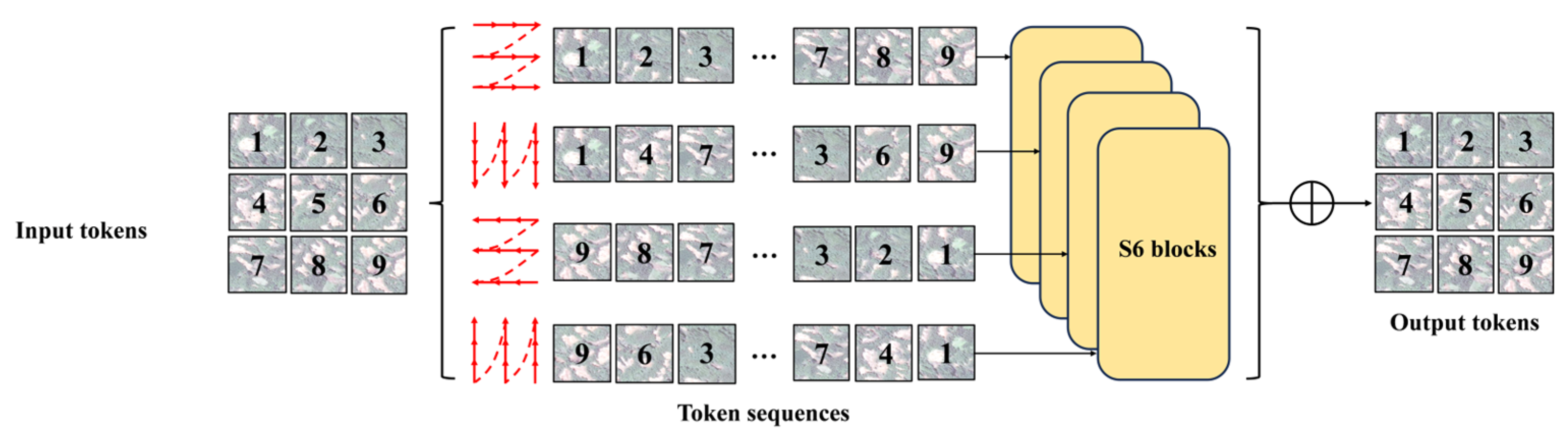
To adapt SSMs to vision tasks, we introduce a parallel VSSMEncoder branch to capture large-context representations from remote-sensing imagery. The VSSMEncoder is composed of stacked VSSBlocks, each including pre-normalization, a four-directional state-space modeling (4-dir SSM) module, and a residual connection (Figure 1b). Specifically, given an input feature map, channels are first expanded and processed by a depthwise convolution to inject local inductive bias. Next, a four-directional selective scan is performed along the horizontal and vertical axes and their reverse directions, producing four directional feature representations (Figure 2). These directional outputs are then merged (by summation), followed by normalization and a gating mechanism that modulates the fused features, which are finally projected back to the original channel dimension.
This 4-dir SSM design is intended to provide two practical benefits for large-scene segmentation. First, the computational and memory complexity scales approximately linearly with the sequence length, which avoids explicitly constructing dense attention matrices and is therefore compatible with large-resolution tiled processing. Second, scanning along both axes in forward and reverse directions enables information propagation across the entire feature map, which is designed to support global semantic interaction beyond local windows and to mitigate discontinuities that may arise in patch-wise inference.

2.2. Cross-Scale Fusion (CSF)

To couple the local semantic features from the convolutional branch with the global contextual features produced by the VSSMEncoder branch [32], we design a Cross-Scale Fusion (CSF) module that performs explicit alignment and fusion at multiple scales (Figure 1c). Specifically, at each scale level i , we take the ResNet feature B i and the VSSM feature F i . The VSSM feature is first projected to a matched channel dimension and spatially aligned to B i via bilinear interpolation. The aligned features are then concatenated along the channel dimension and processed by a 3 × 3 convolution followed by GroupNorm and ReLU for channel mixing and compression, yielding the fused feature U i :
U i = ϕ ( G N ( C o n v 3 × 3 ( [ B i F ^ i ] ) ) )
where [ ] denotes channel-wise concatenation, F ^ i is the channel-projected and spatially aligned VSSM feature, G N ( ) is GroupNorm, and ϕ ( ) is the ReLU activation.
This fusion strategy is designed to reconcile feature discrepancies across branches (e.g., resolution and channel statistics) through an explicit alignment–interaction pathway, rather than directly combining features by element-wise addition. By performing fusion stage-by-stage across multiple scales, CSF facilitates information exchange between shallow texture/boundary cues and deeper semantic/contextual representations within a unified feature space. In addition, GroupNorm is adopted to reduce sensitivity to batch size and to stabilize optimization when fusing features with different distributions. Overall, CSF serves as a lightweight mechanism to support local–global collaboration and multi-scale consistency in large-scene landslide segmentation under tiled processing.

2.3. Deformable Residual Block (DRB)

To enhance geometry-adaptive refinement for irregular landslide boundaries and small targets, we attach a Deformable Residual Block (DRB) after the fused features at each scale [33], as illustrated in Figure 1d. In a standard 2D convolution, a regular sampling grid R is used to sample the input feature map. For an output location p 0 on the feature map y , the convolution is computed as follows:
y ( p 0 ) = p n R w ( p n ) x ( p 0 + p n )
where p n R denotes the sampling offsets in the convolution kernel and w ( p n ) is the corresponding weight.
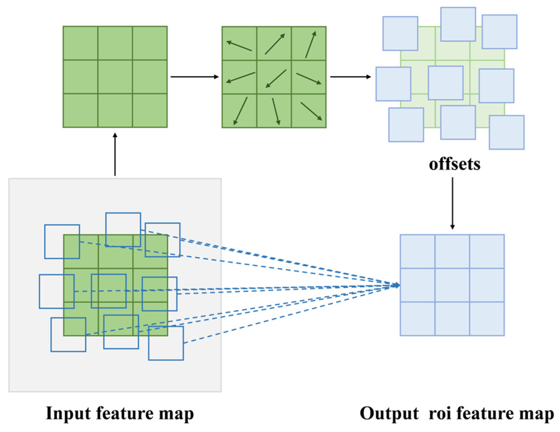
Deformable convolution introduces learnable offsets Δ p n to adapt the sampling locations from the regular grid points p 0 + p n to irregular positions p 0 + p n + Δ p n , leading to the following:
y ( p 0 ) = p n R w ( p n ) x ( p 0 + p n + Δ p n )
Because Δ p n is generally fractional, the feature value at the sampled position is obtained by bilinear interpolation:
x ( p ) = q G ( q , p ) x ( q )
where p = p 0 + p n + Δ p n , q traverses integer coordinates on the input feature map, and the interpolation kernel G ( p , q ) can be decomposed as follows:
G ( q , p ) = g ( q x , p x ) g ( q y , p y )
g ( a , b ) = max ( 0 , 1 | a b | )
This interpolation is non-zero only at the four neighboring integer locations around p , maintaining computational efficiency.
Implementation of DRB: In our DRB, a 3 × 3   convolution predicts the offset field Δ p n from the input features, followed by a deformable convolution for geometry-adaptive sampling. The output is further processed by GroupNorm and ReLU and combined in a residual manner to refine the fused representation (Figure 3). To promote stable optimization, the offset prediction branch is initialized to produce near-zero offsets at the beginning of training, so the block starts from regular sampling and progressively learns geometry-adaptive adjustments. Overall, DRB is designed to provide boundary-aware refinement under multi-scale decoding, enabling the network to better adapt to jagged, tortuous contours and slender structures commonly observed in landslide regions.

2.4. Data Source

This study adopts the CAS Landslide Dataset, a recently released large-scale multi-sensor benchmark designed for deep-learning-based landslide recognition [34]. The dataset contains 20,865 RGB remote-sensing images with pixel-level annotations, covering nine geographic regions and integrating multi-source data from both UAV (unmanned aerial vehicle) and SAT (satellite) imagery. All images are provided as 512 × 512 TIFF tiles, where landslide and non-landslide pixels are labeled as 1 and 0, respectively [32].
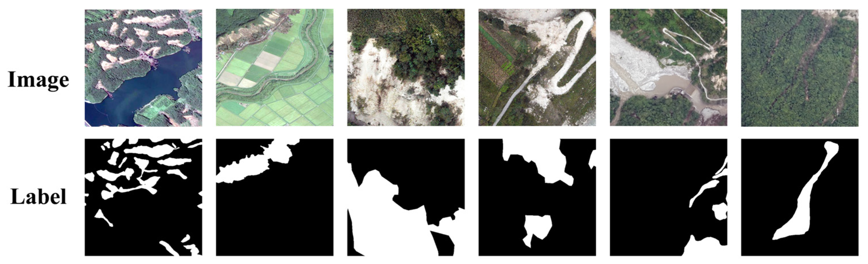
The dataset is constructed following a quality-control workflow, including multi-source image acquisition, expert-assisted annotation, and combined automated/manual screening [34]. Images with large blank areas, extremely low proportions of landslide pixels, severe cloud cover, or obvious stitching seams are excluded by the dataset provider. Figure 4 shows representative examples (UAV imagery and corresponding landslide masks), illustrating that landslides in this benchmark vary substantially in spatial distribution, morphology, and scale, and that complex backgrounds and topographic relief further increase the difficulty of precise delineation.
Data usage and splits: For the in-domain experiments, we select three representative subsets from the CAS Landslide Dataset to build the training/validation sets: Hokkaido Iburi-Tobu (SAT, 3.0 m), Moxi town (UAV, 0.2 m), and Moxitaidi (UAV, 0.6 m). These regions cover diverse geomorphological conditions and landslide-triggering mechanisms:
Hokkaido Iburi-Tobu (Japan, SAT 3.0 m): dominated by earthquake-induced landslides, spanning mountains, plateaus, and coastal plains. High vegetation coverage and steep slopes yield large deposits with clear but irregular boundaries.
Moxi town (Luding County, Sichuan, China, UAV 0.2 m): a high-mountain canyon region where rainfall-induced shallow landslides are common. Landslides are often irregular, numerous, and spatially scattered, posing challenges for small-object delineation and boundary transitions.
Moxitaidi (near Moxi Town, Sichuan, China, UAV 0.6 m): a high terrace in the Dadu River Basin (approximately 1600–2000 m elevation), surrounded by steep slopes. This area is influenced by tectonic activity near the Kangding–Luding seismic zone, where landslides can be triggered by earthquakes, heavy rainfall, and seasonal freeze–thaw cycles. Both deep-seated landslides and dense shallow failures occur, and diverse landforms (terraces, gullies, grass slopes, sparse forests) introduce complex visual patterns.
To improve training efficiency and mitigate extreme class imbalance, we filter out tiles with extremely small landslide areas (landslide pixel ratio < 1%) from the selected in-domain subsets. This results in 1000 in-domain samples used for model development, which are then split into training/validation/testing sets with an 8:1:1 ratio (i.e., 800/100/100).
Cross-domain test sets: To assess generalization beyond the in-domain distribution, we additionally evaluate the trained model on two independent cross-domain subsets, which are not used for training or validation:
Jiuzhai Valley (UAV, 0.2 m): a seismically induced landslide-prone area characterized by distinctive lithology (e.g., limestone and dolomite), high-altitude canyon landforms, and a subalpine climate. Vegetation is dominated by alpine coniferous forests and shrubs, resulting in image appearances that differ from the in-domain subsets.
Bijie (SAT, 0.8 m): a mountainous karst-affected region in southwest China with strong terrain relief and heterogeneous land cover. Compared with the in-domain subsets, Bijie exhibits different sensor characteristics and background textures (e.g., exposed rock, cultivated slopes, and patchy vegetation), providing an additional setting to examine cross-domain behavior under distinct resolution and imaging conditions.
For cross-domain evaluation, we use 200 tiles for Jiuzhai Valley and 200 tiles for Bijie as independent test sets. For completeness, Table 1 also reports the positive-to-negative pixel ratios for these cross-domain subsets using the same statistical protocol, facilitating a consistent comparison of class imbalance across regions.
Overall, the configuration above supports both in-domain training/validation/testing and cross-domain testing, enabling evaluation of model performance across diverse geomorphological settings, triggering factors, and sensor conditions.


3. Experiments and Analysis

3.1. Experimental Loss Function

To optimize the pixel-level prediction results for landslide segmentation, this study adopts a combined loss function of Intersection-over-Union Loss (IoU Loss) and Dice Loss [35,36]. Let the predicted mask be p     [ 0 ,   1 ] H × W and the ground-truth mask be g     { 0 ,   1 } H × W . First, compute the intersection I   =   i p i g i and the union U   =   i p i + i g i I . The IoU loss is then defined as follows:
L I o U = 1 I + ϵ U + ϵ
where ε is a smoothing term to avoid division by zero. To improve sensitivity to small targets and boundary regions, Dice Loss is introduced:
L D i c e = 1 2 I + ϵ i p i + j g j + ϵ
The final total loss is defined as the weighted sum of the two:
L = λ L I o U + ( 1 λ ) L D i c e
where λ = 0.5 represents an equal-weight combination. This combined loss takes into account both global region overlap and local boundary accuracy, improving overall segmentation consistency while mitigating the impact of class imbalance, thereby producing more refined landslide mask boundaries.

3.2. Evaluation Metrics

To verify the accuracy and performance of the model on landslide imagery, this study evaluates segmentation results using Pixel Accuracy (PA), Recall, Intersection over Union (IoU), and F1-score as key metrics [37]. In addition, the model’s parameter count (Params) and computational complexity (GFLOPs) are reported to comprehensively assess both its accuracy and efficiency [38].
In these formulations, TP (True Positive) represents pixels that are truly landslides and correctly predicted as landslides, while TN (True Negative) represents pixels that are truly non-landslides and correctly predicted as non-landslides. FP (False Positive) refers to pixels that are actually non-landslides but incorrectly predicted as landslides, and FN (False Negative) refers to pixels that are truly landslides but incorrectly predicted as non-landslides. These four quantities form the basis for all subsequent metric calculations and comprehensively reflect the model’s capability in correct identification, false alarms, and missed detections.
P A = T P + T N T P + T N + F P + F N
PA (Pixel Accuracy) measures the proportion of correctly predicted pixels over the total number of pixels and is the most basic evaluation metric in segmentation models [39]. In landslide segmentation tasks, PA reflects the model’s overall classification accuracy across the entire remote-sensing image, indicating how well the model distinguishes landslide and non-landslide areas at the pixel level.
R e c a l l = T P T P + F N
Recall measures the proportion of pixels that are truly landslides and are correctly predicted as landslides [40]. In landslide segmentation tasks, this metric reflects the model’s ability to detect all landslide areas—often referred to as its “completeness.” A higher Recall indicates fewer missed detections of landslide regions, meaning the model can more comprehensively identify landslides within the remote-sensing image.
F 1 = 2 T P 2 T P + F P + F N
The F1-score is the harmonic mean of Precision and Recall, providing a comprehensive measure of the model’s ability to both “detect accurately” and “detect completely” [41]. In landslide segmentation tasks, the F1-score offers a more balanced evaluation of the model’s performance in reducing false positives while minimizing missed detections, thus reflecting the trade-off between accuracy and completeness in landslide identification.
I o U = T P T P + F P + F N
IoU (Intersection over Union) represents the ratio of the intersection to the union between the predicted region and the ground-truth region and is one of the core evaluation metrics in semantic segmentation tasks [42]. In landslide segmentation, a higher IoU indicates that the predicted landslide boundaries align more closely with the true boundaries, meaning the model achieves better spatial accuracy and produces masks that more precisely match the actual landslide shapes.
P b = | B p D r ( B g ) | | B p |
R b = | B g D r ( B p ) | | B g |
B F 1 = 2 P b R b P b + R b
Boundary F1 (also referred to as Boundary F-score, BFscore) is a boundary-sensitive segmentation metric that measures how well the predicted mask boundary aligns with the ground-truth boundary in the image space. Here, B p and B g denote the sets of boundary pixels extracted from the predicted and ground-truth masks, respectively, and D r ( ) represents a tolerance band with radius r (e.g., obtained by morphologically dilating the boundary by r pixels) to accommodate slight registration errors and pixel quantization effects; P b and R b are the boundary precision and boundary recall, and B F 1 is their harmonic mean. In landslide segmentation, conventional metrics such as IoU and region-level F1 mainly emphasize area overlap, whereas Boundary F1 directly evaluates geometric boundary alignment and is more sensitive to irregular contours, thin or fragmented landslide shapes, and boundary over-smoothing/over-expansion, thereby providing a more targeted assessment of boundary delineation quality and spatial localization accuracy and offering more direct quantitative evidence for boundary-refinement and irregular-boundary modeling modules.
P a r a m s = l = 1 L P a r a m e t e r ( l )
Params represent the total number of trainable parameters in a model and are an important indicator of model complexity and storage cost [43]. In landslide segmentation tasks, a smaller parameter count means the model is more lightweight and therefore better suited for deployment on disaster-monitoring devices with limited computational and memory resources.
F L O P s c o n v   = 2 H o u t   W o u t   C o u t   C i n   g K h K w
G F L O P s = N u m b e r   o f   F l o a t i n g   P o i n t   O p e r a t i o n s 10 9
GFLOPs is defined as the total number of floating-point operations for a single-image forward pass divided by 10 9 . Here, H out and W out denote the output feature map height and width, C out the number of output channels, C in the number of input channels, K h and K w the convolution kernel size, and g the number of groups. The coefficient 2 comes from MAC (Multiply–Accumulate), with the convention 1   MAC = 1 multiplication +   1 addition = 2 FLOPs. Unless otherwise specified, FLOPs are computed under a default input of 512 × 512 × 3 , and the counting scope mainly covers convolutional and linear layers. We note that GFLOPs is a profiler-based theoretical indicator; for models involving customized operators (e.g., state-space scanning), FLOPs profilers may have incomplete or inconsistent coverage. Therefore, GFLOPs is used as a reference measure of computational complexity, and we additionally report measured deployment-oriented indicators (e.g., inference latency and peak GPU memory) to provide a fair and practical assessment of efficiency.
In landslide segmentation, higher GFLOPs typically imply greater computational cost and potentially stronger representational capacity, whereas lower GFLOPs suggest higher efficiency and easier deployment (useful for large-area tiled mapping and emergency applications). In practice, one must balance boundary accuracy, small-object recall, cross-region semantic coherence, and computational overhead. GFLOPs measure the floating-point operations required for a single forward inference pass, expressed in billions [44]. In landslide segmentation tasks, lower GFLOPs indicate that the model can process large-scale remote-sensing imagery more efficiently, offering better practical applicability.
Besides Params and GFLOPs, we additionally report deployment-oriented efficiency indicators, including measured inference latency (ms/image), peak GPU memory usage (GB), and (optionally) throughput (images/s), to quantify the accuracy–efficiency trade-off under practical constraints. Latency is measured with batch size 1 after a warm-up phase, and peak memory is recorded as the maximum GPU memory allocated during inference; throughput is computed as the number of processed images per second under the same input size and hardware/software settings.
| Δ | = | | Δ p | | 2 = ( Δ x ) 2 + ( Δ y ) 2
Δ (offset magnitude) measures the displacement strength of the learned deformable sampling offsets, where Δ p = ( Δ x , Δ y ) denotes the predicted 2D offset vector (in pixel units under the current feature-map scale). In landslide segmentation, a moderate increase in Δ near irregular boundaries is often expected, as deformable sampling adapts to contour geometry; meanwhile, consistently excessive Δ may indicate overly aggressive sampling and potential feature aliasing, especially in dense or complex-texture scenes.
P 95 ( | Δ | ) = Q u a n t i l e 0.95 ( { | Δ | i } i = 1 N )
P 95 ( Δ ) reports the 95th percentile of offset magnitudes over all sampled positions (and/or all deformable sampling points), capturing the upper-tail behavior of the offset distribution while being less sensitive to extreme outliers than the maximum value. In practice, P 95 ( Δ ) serves as a robust indicator for detecting offset drift or sporadic overly large offsets that may occur in dense distributions or complex-boundary regions.
R a t i o ( | Δ | > r ) = 1 N i = 1 N I ( | Δ | i > r )
R a t i o ( Δ   > r ) measures the proportion of offsets whose magnitudes exceed a predefined threshold r (in pixels under the current feature scale, e.g., r = 2.0 ), where I ( ) is an indicator function and N is the number of sampled offsets. This metric directly quantifies how frequently large offsets occur. A low ratio suggests stable and conservative deformations, whereas an abnormally high ratio may imply offset explosion or drift, which can undermine the reproducibility and applicability of deformable modeling in dense or complex-texture scenarios.

3.3. Experiment Settings

All the experiments were conducted on a server equipped with eight NVIDIA Tesla T4 GPUs (15 GB memory per GPU). Multi-GPU parallel training was adopted to accelerate convergence. The deep learning framework was PyTorch (version 1.10.0), with CUDA version 12.5. The AdamW optimizer was used with a weight decay of 0.05 and an initial learning rate of 0.0002. A cosine annealing scheduler combined with a linear warm-up strategy was employed to gradually decay the learning rate, ensuring stable convergence during the later stages of training.
The dataset was split into training/validation/testing sets in an 8:1:1 ratio, and the model was trained for 100 epochs. The total batch size was set to 16 (evenly distributed across GPUs), and the gradients and parameters were synchronized across GPUs during training. These hyperparameters were determined through multiple rounds of tuning to balance convergence speed and segmentation performance. For the proposed dual-branch architecture, the CNN branch and the VSSM branch were optimized jointly in an end-to-end manner using the same segmentation objective. Cross-branch interactions (e.g., stage-wise feature exchange and cross-scale alignment) were implemented as differentiable operations, so gradients were back-propagated through both branches without stop-gradient or branch-wise freezing. We did not introduce additional gradient-balancing losses; instead, we applied a unified optimizer and learning-rate schedule to all the parameters, and the training procedure remained stable in our experiments.
During training, data augmentation was applied, including random flipping, rotation, and brightness perturbations, to enhance model generalization. The mean Intersection-over-Union (mIoU) was monitored on the validation set, and early stopping was applied when the performance showed no improvement for several consecutive epochs to prevent overfitting. The weights that achieved the best validation performance were selected as the final model for testing.
To characterize deployment-oriented efficiency, we additionally benchmarked inference under a unified protocol. Unless otherwise specified, inference was evaluated on a single Tesla T4 GPU with input size 512 × 512 and batch size 1, which is consistent with the commonly used tile-based processing paradigm for large-scale remote-sensing imagery. For each model, we first performed a fixed number of warm-up iterations to eliminate initialization overhead and then measured the runtime over multiple forward passes; the reported latency (ms/image) is the average over the timed runs. The timing includes model forward and the standard post-processing in our pipeline (e.g., sigmoid activation and resizing), while excluding disk I/O. Peak GPU memory (GB) is recorded as the maximum allocated memory during inference, and throughput (images/s) is computed under the same configuration. This unified setting enables a fair comparison of accuracy–efficiency trade-offs across different methods under practical constraints.

3.4. Experimental Comparison Models

To comprehensively evaluate the proposed method for landslide segmentation, we selected representative comparison models spanning CNN-based, Transformer-based, and recent SSM/Mamba-based segmentation architectures.
The CNN baselines include the classic U-Net [45] and DeepLabV3+, representing convolution-centered encoder–decoder designs for local feature modeling. The Transformer baselines include SegFormer [46], Mask2Former [47], and Swin Transformer [48], which incorporate self-attention for broader-context modeling in segmentation. In the emerging SSM direction, we further include RS3Mamba [27] and VM-UNet [49], which integrate Mamba-style state-space modeling into segmentation pipelines to enable global information propagation with favorable computational characteristics.
For clarity, although RS3Mamba and VM-UNet also explore SSM/Mamba-based global modeling, DFmamba places additional emphasis on explicit stage-wise cross-scale aligned interaction (CSF) to reconcile feature distributions between local texture/boundary cues and global contextual representations and further incorporates decoder-side geometry-adaptive boundary refinement (DRB) and shallow high-frequency detail preservation (MFP) to address irregular boundaries and small-object detail retention in landslide segmentation. Unless otherwise specified, all the comparison models were trained and evaluated under the same data split and experimental protocol described in Section 3.3 to ensure a fair accuracy–efficiency comparison.

4. Results

4.1. Benchmark Performance Evaluation

To verify the effectiveness of DFmamba, we conducted benchmark comparisons under a same-source split, where the dataset was randomly divided into training/validation/testing sets with an 8:1:1 ratio. Table 2 reports both segmentation accuracy and deployment-related complexity indicators, including parameters (Paras), GFLOPs, average inference latency (ms/image), and peak GPU memory usage (GB). In addition to region-based metrics (Precision, Recall, F1-score, and IoU), we further introduce Boundary F1 to explicitly measure boundary alignment quality, which is critical for landslide mapping with irregular edges.
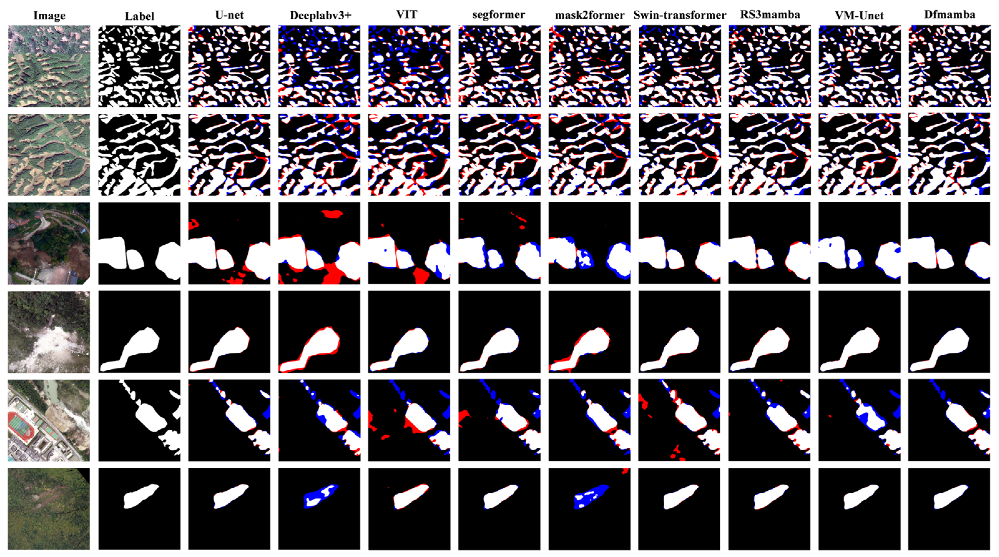
Overall, As shown in Figure 5, DFmamba achieves the best performance across all the reported accuracy metrics. Specifically, DFmamba reaches an F1-score of 0.9351 and an IoU of 0.8781, outperforming the second-best model RS3Mamba (F1 = 0.9237, IoU = 0.8583). This corresponds to an absolute gain of +1.14 percentage points in F1 and +1.98 percentage points in IoU. More importantly, DFmamba yields a substantially higher Boundary F1 of 0.6854, improving over RS3Mamba (0.6032) by +0.0822, indicating markedly better boundary continuity and edge adherence.
From an efficiency perspective, although DFmamba adopts a stronger dual-branch representation and thus uses more parameters than several lightweight baselines, it remains deployment-friendly in practice. DFmamba achieves 22.58 ms/image latency with 0.61 GB peak memory, which is faster and more memory-efficient than RS3Mamba (33.27 ms/image, 0.90 GB). Compared with typical Transformer-based baselines, DFmamba also delivers better region overlap and boundary consistency while keeping latency and memory usage within a comparable range, demonstrating a favorable accuracy–efficiency balance for high-resolution landslide segmentation.
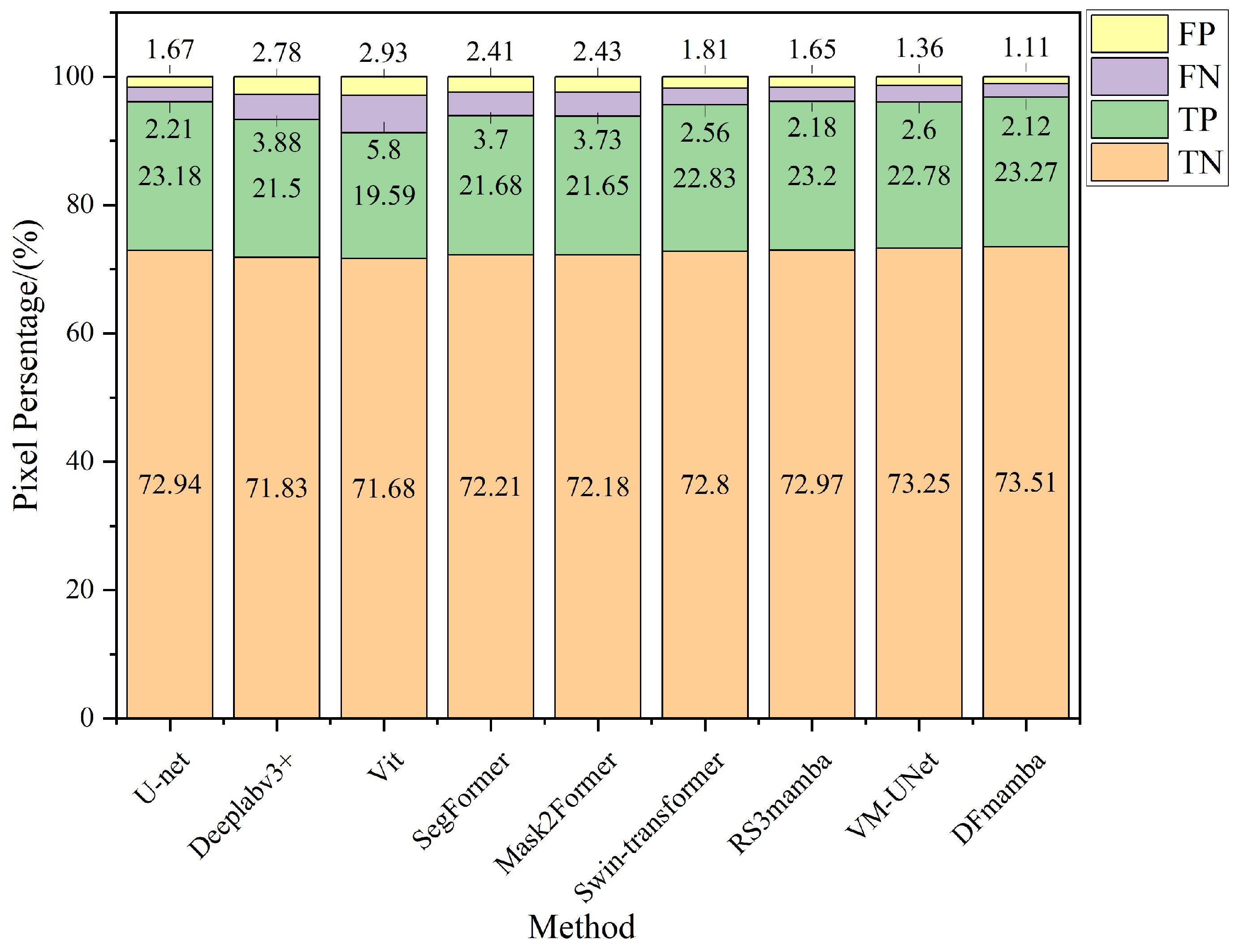
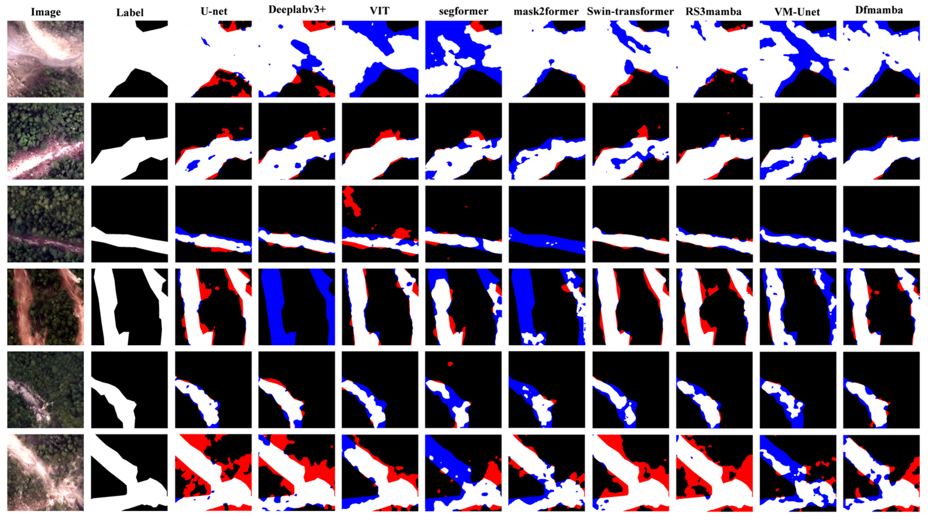
Figure 6 shows segmentation comparisons on representative samples. It can be seen directly that DFmamba produces fewer false positives and false negatives, with more continuous predicted boundaries and more complete coverage of landslide areas. Table 2 presents the confusion matrix statistics for the test set. DFmamba achieves a True Positive Rate (TPR) of 67.72% and a True Negative Rate (TNR) of 24.78%, resulting in an overall pixel accuracy (TP + TN) of 92.5%. Its False Negative Rate (FNR) and False Positive Rate (FPR) are only 3.49% and 4.01%, respectively, both lower than those of the representative models listed in Table 2. These results indicate that DFmamba not only maintains high accuracy but also effectively suppresses missed detections and false alarms, demonstrating higher stability and reliability for landslide segmentation in complex remote-sensing imagery.
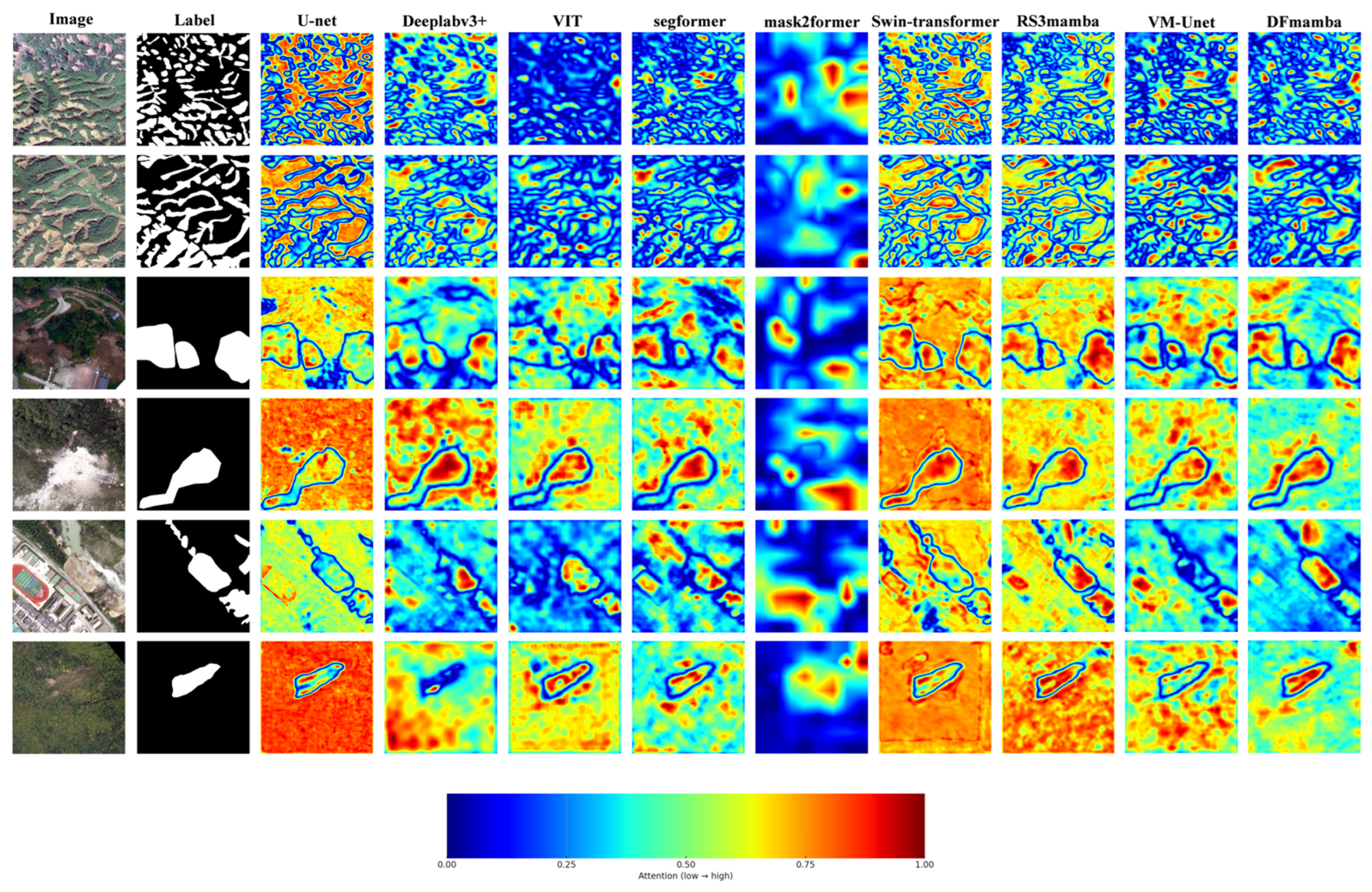
To further qualitatively analyze the model’s ability to perceive key information, we applied Gradient-weighted Class Activation Mapping (Grad-CAM) to visualize the model’s sensitivity to different regions in the image during the output stage. Grad-CAM generates heatmaps based on the gradient information of the model’s final convolutional layer, highlighting the regions the model focuses on most. As shown in Figure 7, U-Net, DeepLabv3+, Swin-Transformer, and RS3Mamba display relatively strong responses to background areas in some samples. ViT, SegFormer, Mask2Former, and VM-UNet are able to cover the main landslide body but still allocate attention to irrelevant regions in certain cases. In contrast, DFmamba shows highly concentrated attention on the landslide body and its boundaries, with background activation effectively suppressed. This observation is consistent with the higher F1/IoU scores and lower FP/FN rates reported in Table 1 and Table 2, further confirming the superior separability and reliability of the proposed method in complex geomorphological scenarios.

4.2. Scene-Wise Evaluation

To measure the robustness of different methods at a finer granularity, we group and evaluate the test samples along three dimensions: Area Proportion (S), Geometric Complexity (G), and Quantity (N). The metric definitions are as follows (using the binary mask M to represent landslide pixels):
ρ S = 1 ( M > 0 ) | M |
N o b j = c o n n e c t e d _ c o m p o n e n t s ( M )  
e = L max L min + ε         ( ε = 10 6 )
ϕ = P 2 π A
where ρ S denotes the area proportion; N obj is the number of connected landslide objects; e is the elongation ratio (major/minor axis length); and ∅ is the shape index (A for area, P for perimeter). Based on these, the grouping criteria are given in Table 3.
The test set samples were divided into eight scenarios, and the mean values of each model’s metrics were calculated within each group, as shown in Table 4. The results reveal that the scenarios S-Small, G-Complex, and N-Dense pose significant challenges for all the methods. For S-Small, the small-area landslides suffer from class imbalance and low signal-to-noise ratio, making them prone to missed detections. For G-Complex, the samples have tortuous and irregular boundaries, which leads to reduced boundary localization accuracy and mask closure quality. In N-Dense cases, landslides are adjacent or overlapping, causing confusion between background and target and resulting in adhesion and false positives.
Across these challenging scenarios, DFmamba consistently demonstrates stable advantages and strong control over false positives and false negatives. In the G-Complex group, DFmamba achieves a score of 0.8988, the highest in this group, which is an absolute improvement of 0.0079 (≈0.79 percentage points) over U-Net (0.8909). This shows that for landslides with tortuous, irregular boundaries, DFmamba is better at maintaining mask closure and boundary continuity. In the S-Small group, DFmamba reaches 0.9142, which is comparable to the best VM-UNet (0.9215) and higher than the second-best U-Net (0.9137). In the N-Dense group, DFmamba scores 0.7629, slightly lower than U-Net (0.7834) and VM-UNet (0.7810). However, combined with the confusion matrix results in Figure 6, it can be observed that DFmamba achieves lower FP/FN proportions, fewer false positives and missed detections, and better coherence of predicted regions. This demonstrates that when multiple instances are adjacent or slightly overlapping, the model more robustly suppresses boundary interference and background confusion.
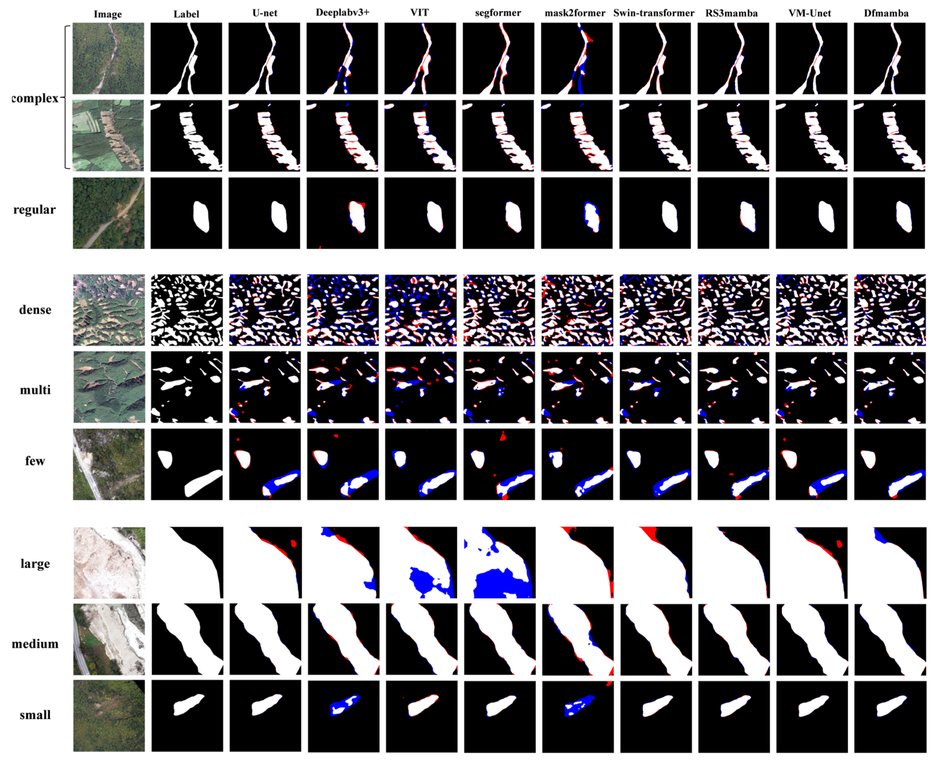
Figure 8 presents a visualization comparison of typical samples in the three challenging scenarios (the color coding is the same as in Figure 2). It can be clearly observed that in the G-Complex and S-Small scenarios, DFmamba produces significantly fewer false positives and false negatives, with smoother and more closed boundaries. In the N-Dense scenario, although the overall difficulty is higher, DFmamba can still effectively suppress background misactivation and maintain separation between adjacent landslides. Taken together, these comparisons show that DFmamba has substantial advantages in complex-shape and small-scale scenarios. Although it exhibits a slight overall score disadvantage in densely distributed scenarios, it compensates with lower false positives/false negatives and higher structural integrity, demonstrating more reliable discrimination and generalization ability under challenging conditions.
4.3. Cross-Domain Generalization Test

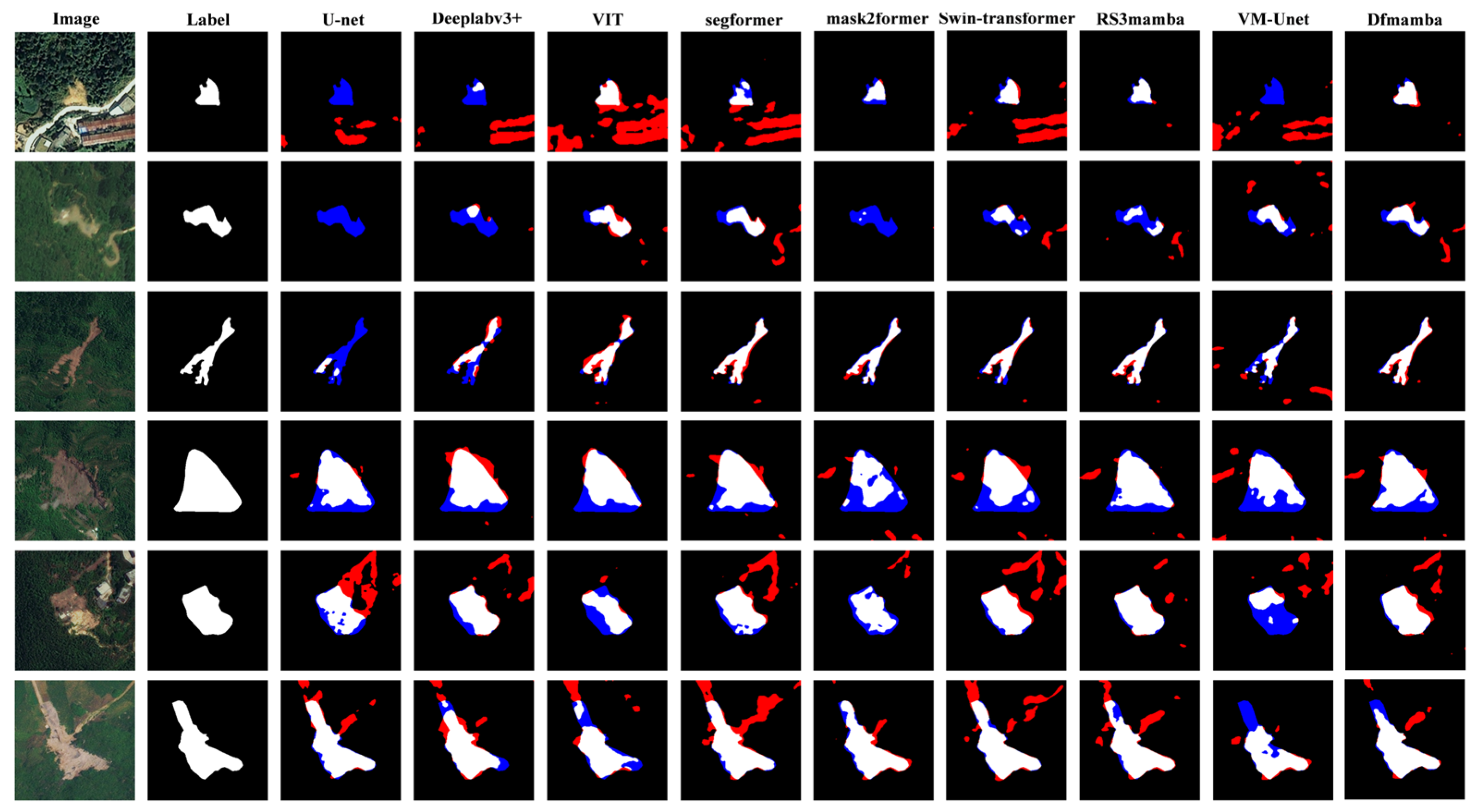
To evaluate the robustness of the proposed method under out-of-domain conditions, we trained all the models on the same source training set and conducted zero-shot testing on two target domains without any fine-tuning: (i) the Jiuzhai Valley dataset and (ii) the Bijie dataset, which differs from the source domain in geomorphology, surface texture, vegetation coverage, and imaging conditions. The quantitative results are reported in Table 5 and Table 6 (Jiuzhai Valley; Bijie), and qualitative comparisons are shown in Figure 9 and Figure 10.
Overall, all the methods suffer performance drops when transferred across domains, indicating that cross-domain landslide segmentation remains challenging due to domain shifts in illumination, texture, and terrain-induced appearance variations. Nevertheless, DFmamba consistently demonstrates strong transferability on both target domains. On Jiuzhai Valley (Table 5), DFmamba achieves the highest IoU (0.6364) and the best Boundary F1 (0.4302) among all the methods, showing improved region overlap and boundary adherence in complex mountainous scenes. Notably, DFmamba maintains a competitive F1-score of 0.7572, which is on par with the strongest baseline (RS3Mamba: 0.7578), while exhibiting superior boundary quality and more stable spatial consistency.
On Bijie (Table 6), DFmamba delivers the strongest overall results on all the evaluated metrics, achieving a precision of 0.9435, a recall of 0.7678, an F1-score of 0.8581, and an IoU of 0.7514, together with the highest Boundary F1 of 0.5137. Compared with the second-best model, RS3Mamba, DFmamba improves the F1-score by 0.0238 and the IoU by 0.0357 while further increasing Boundary F1 by 0.0269. These consistent gains suggest that the proposed deformable boundary modeling and multi-scale fusion enhance robustness to domain shifts, yielding more reliable segmentation under varying illumination, texture, and terrain-induced appearance changes.
Figure 9 and Figure 10 further support the quantitative findings. In the Jiuzhai Valley scenes with highly undulating terrain and complex background textures, DFmamba produces predictions that align more closely with true landslide extents, with fewer boundary breaks and reduced over-expansion. In contrast, several baselines exhibit false activations or distorted boundaries in regions affected by shadows, exposed soil, or vegetation textures. Similar trends can be observed on the Bijie dataset, where DFmamba yields more complete landslide coverage and cleaner boundaries, demonstrating improved robustness and practical value for cross-domain landslide mapping in complex geomorphological environments.

4.4. Input Size Sensitivity Analysis

In the input size comparison (Table 7), we tested four block sizes—128 × 128, 256 × 256, 512 × 512, and 1024 × 1024—while comparing parameter counts (Params) and computational cost (GFLOPs). The results show that Params remain constant across all the sizes, while the GFLOPs increase monotonically with input size. ViT, SegFormer, Swin-Transformer, and Mask2Former exhibit a more pronounced GFLOPs increase at 1024 × 1024, and RS3Mamba and VM-UNet also show a significant rise with input size. In contrast, DFmamba’s GFLOPs grow approximately linearly with the number of pixels and remain relatively low among the models at the 1024 × 1024 scale, showing more controllable computational cost across all three input sizes. Based on the Params/GFLOPs comparison in Table 7, we selected 256 × 256 as the default input size for subsequent experiments to strike a stable balance between resource consumption and fairness of comparison, with larger input sizes used only when a broader field of view is required. Overall, from a purely computational cost perspective, DFmamba demonstrates superior efficiency performance across multiple input scales.

4.5. Ablation Study

To quantify the contribution of each component in DFmamba and to better understand its behavior under different scene conditions, we conducted systematic ablation experiments using the same training/validation protocol. The results are summarized in Table 8, which compares backbone-only variants and progressively added modules. When using only the CNN backbone, the model achieves the lowest performance (F1 = 0.8892, IoU = 0.8005). Adding the VSSM encoder strengthens long-range dependency modeling and large-scale morphological perception, improving F1/IoU to 0.8958/0.8112. Introducing CSF further promotes multi-resolution feature alignment and fusion, leading to clearer boundary evidence and improved region overlap. Finally, incorporating DRB markedly improves the delineation of irregular boundaries and small landslides via deformable sampling, and the full configuration achieves the best overall results (F1 = 0.9351, IoU = 0.8781, Boundary F1 = 0.6854).
Beyond the overall metrics, we further examine where DRB contributes most by performing a stratified analysis (Table 9). Across all the strata, adding DRB consistently improves accuracy and boundary quality. The gains are most pronounced for small landslides (ΔF1 = +0.0228, ΔIoU = +0.0272, ΔBoundary F1 = +0.0646) and complex scenes (ΔF1 = +0.0191, ΔIoU = +0.0254, ΔBoundary F1 = +0.0603), confirming that deformable boundary modeling is particularly beneficial when boundaries are highly curved, fragmented, or easily confused with background textures. In contrast, improvements are more modest in regular or large-object strata, indicating that DRB mainly acts as a boundary- and detail-aware refinement mechanism rather than simply enlarging coarse regions.
To explain the stability of deformable sampling under different domain conditions, we report offset-field magnitude statistics at the highest-resolution DRB stage (closest to the prediction head), which most directly affects final boundary alignment and small-object delineation. As reported in Table 10, the offset magnitudes remain controlled across the strata, with the mean |Δ| generally within 0.49–0.71 (in pixel units at the feature-map resolution). We further diagnose potentially over-large offsets using an exceedance threshold r = 2.0; the exceedance ratios remain low (1.21–4.49%), suggesting that the learned sampling is adaptive yet stable, avoiding overly aggressive deformation that could cause aliasing in dense or complex-texture scenes.
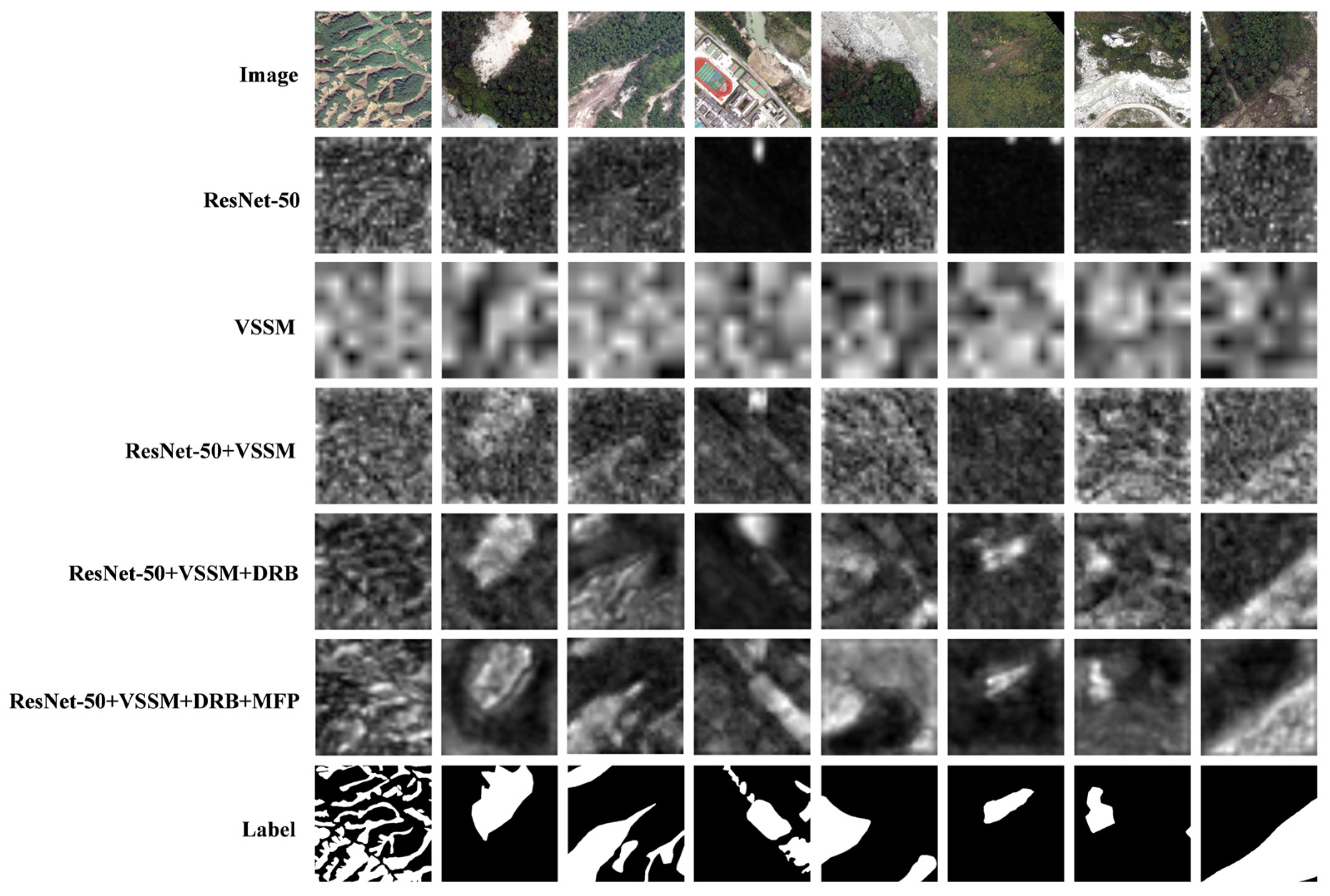
Figure 11 provides qualitative evidence consistent with the findings above. From top to bottom, feature responses become progressively more compact and boundary-aware: noisy and diffuse activations with blurred edges are gradually replaced by coherent structures and clearer contours. This effect becomes particularly evident after introducing DRB and integrating all the modules, where responses to elongated landslides and irregular boundaries are more focused, while boundary breaks and spurious artifacts are significantly reduced.

5. Discussion

This study presents DFmamba, a deformable dual-branch visual state-space network tailored for high-resolution landslide segmentation under practical tiled/sliding-window inference. The method is designed to jointly address four interrelated difficulties in operational mapping: (i) semantic inconsistency across large scenes under tiled processing, (ii) jagged and irregular landslide boundaries, (iii) the loss of low-level high-frequency details that are critical for small landslides and transitional boundary zones, and (iv) strict deployment constraints on latency and GPU memory in emergency-response scenarios. To this end, DFmamba integrates a dual-branch encoder to combine local texture/boundary cues with global long-range propagation and further introduces explicit mechanisms for stage-wise cross-scale aligned interaction (CSF), geometry-adaptive boundary refinement (DRB), and shallow-detail preservation (MFP) to better fit irregular geometry and multi-scale characteristics under tiled inference.
Quantitative benchmarking indicates that DFmamba achieves the best segmentation accuracy while maintaining a favorable deployability profile. In the same-source split evaluation, DFmamba reaches F1 = 0.9351 and IoU = 0.8781, outperforming the second-best method (RS3Mamba) by +1.14 pp (F1) and +1.98 pp (IoU). Importantly, DFmamba yields a substantially higher Boundary F1 = 0.6854 (vs. 0.6032), demonstrating stronger boundary continuity and edge adherence—an aspect that is directly relevant to inventory mapping where irregular margins dominate error patterns. While DFmamba employs a stronger dual-branch representation, it remains deployment-friendly in practice: under a unified inference protocol (T4 GPU, 512 × 512 tile, batch size 1), DFmamba reports 22.58 ms/image latency and 0.61 GB peak memory, which is faster and more memory-efficient than RS3Mamba (33.27 ms/image, 0.90 GB). The inference protocol itself is aligned with real-world remote-sensing pipelines (tile-based processing), and the reported timing includes standard post-processing while excluding disk I/O, improving the interpretability of deployment metrics. Collectively, these results suggest that the proposed design does not pursue accuracy by blindly increasing computation; instead, it improves boundary fidelity and cross-scale robustness while keeping latency and memory within an operationally feasible range.
A central contribution of DFmamba is its explicit focus on irregular-boundary modeling, which is reflected in the Boundary F1 improvements. The ablation results show that adding DRB markedly improves the delineation of irregular boundaries and small landslides via deformable sampling, and the full configuration achieves the best overall performance (F1 = 0.9351, IoU = 0.8781, Boundary F1 = 0.6854). Beyond overall gains, the stratified analysis further reveals that DRB’s improvements are most pronounced for small landslides and complex scenes, which is consistent with the motivation that fixed sampling is insufficient for tortuous margins and fragmented structures. In practice, this means DRB contributes not only to increasing region overlap but also to producing more topologically plausible and contiguous boundaries, thereby reducing over-smoothing and contour mismatch that are common failure modes in high-resolution landslide mapping.
Another key factor is the integration of selective state-space modeling for long-range dependency capture. The ablation indicates that introducing the VSSM encoder improves F1/IoU relative to the CNN backbone, supporting the claim that global propagation helps mitigate semantic discontinuity under tiled processing. However, in high-resolution landslide imagery, global propagation alone is often insufficient: local texture and boundary evidence must remain consistent with global semantics across scales. DFmamba addresses this gap by emphasizing stage-wise cross-scale aligned interaction (CSF), which is explicitly positioned as a differentiator from existing Mamba-based segmentation pipelines. Conceptually, CSF reduces feature distribution mismatch between local detail cues and global contextual representations, improving multi-resolution fusion and contributing to clearer boundary evidence and more coherent region coverage across tiles.
High-frequency shallow cues (e.g., slip traces, fissures, fine collapse edges) are crucial for detecting small landslides and accurately delineating transitional boundary zones, yet they are easily weakened by multi-scale fusion and upsampling. DFmamba includes MFP as an explicit shallow-detail preservation mechanism (described as “shallow high-frequency detail preservation”), complementing the boundary-adaptive refinement of DRB and the global modeling of the VSSM branch. The ablation table includes MFP-related variants, supporting a component-level interpretation that the best performance is achieved when global modeling, cross-scale alignment, boundary refinement, and detail preservation are combined.
While deformable sampling improves geometric adaptability, it may be sensitive in dense-texture scenarios if offsets become unstable. To address this concern and improve reproducibility, this paper introduces an offset-based stability perspective, noting that an abnormally high ratio of large offsets may indicate offset explosion or drift and can undermine applicability in dense or complex-texture cases. This discussion provides an important operational interpretation: DFmamba’s deformable components should not be judged only by accuracy but also by whether deformation behaviors remain stable and controllable under realistic scene complexity.
Despite these promising results, several limitations remain. First, the current evaluation emphasizes a same-source random split protocol, which—while standard—may not fully eliminate spatial correlation in remote-sensing data and thus may yield optimistic estimates compared to cross-region deployment. Second, while the inference protocol and efficiency indicators are carefully defined under the tile-based setting, further profiling on broader hardware settings and large-area mosaicking workflows would strengthen the deployability narrative. Third, although DRB and MFP demonstrably improve complex boundaries and small landslides, challenging cases with dense background textures and highly fragmented terrain still motivate future robustness work—particularly on stabilizing deformable offsets and improving generalization under severe domain shift. Future studies may therefore incorporate (i) broader cross-region multi-scene evaluations, (ii) more diverse sensors or auxiliary modalities (e.g., DEM/SAR where available) to reduce reliance on appearance cues, and (iii) further optimization of the tile inference pipeline (e.g., overlap–blend strategies and memory-aware batching) to improve large-area mapping throughput.

6. Conclusions

This study targets key engineering bottlenecks in high-resolution landslide interpretation—missing large landslide bodies, boundary displacement, and loss of small-scale details—and proposes DFmamba, a deformable dual-branch visual state-space network. DFmamba adopts a parallel “CNN branch + VSSM branch” encoder, where the CNN branch captures local textures and boundary cues, while the VSSM branch performs full-image contextual modeling via selective scanning and linear recurrence, mitigating fragmented understanding and under-coverage induced by windowed/tiled processing.
To enhance contour adherence and detail fidelity in complex geomorphological scenes, DFmamba introduces a Deformable Residual Block (DRB) in the decoder to adaptively align jagged and tortuous boundaries and designs a cross-scale feature alignment and shallow high-frequency injection (MFP) mechanism to explicitly compensate low-level textures and high-frequency edges during deep–shallow fusion and upsampling. Meanwhile, the overall framework achieves global modeling and multi-scale fusion through selective state recursion rather than heavyweight global attention, yielding more controllable computation and improved deployability in operational workflows.
On the CAS Landslide Dataset benchmark with same-source splits, DFmamba achieves the best overall performance (Precision = 0.9678, Recall = 0.9165, F1 = 0.9351, IoU = 0.8781) with a favorable accuracy–complexity trade-off. Compared with the second-best RS3Mamba, DFmamba improves F1/IoU/PA by 0.07%/4.62%/3.32%, indicating more consistent boundaries and higher region overlap.
Stratified evaluations further demonstrate DFmamba’s robustness in challenging scenarios, such as complex-shape boundaries (G-Complex) and small-scale landslides (S-Small) (e.g., 0.8988 in G-Complex), reflecting stronger control over boundary continuity and mask closure. In a zero-shot cross-domain test on the Jiuzhai Valley UAV-0.2 m dataset, DFmamba still maintains leading F1 and IoU (F1 = 0.7572, IoU = 0.6364), suggesting improved adaptability to variations in geomorphology, texture, and imaging conditions. Ablation studies confirm the effectiveness of each component, where the full configuration achieves the highest F1 and IoU (F1 = 0.9351, IoU = 0.8782), validating the contributions of global context modeling, cross-scale alignment, and deformable boundary refinement.
Future work will expand cross-region and cross-sensor validation with more rigorous split protocols, incorporate additional modalities (e.g., DEM/SAR) and geomorphological priors to further suppress background confusion, and improve deployment efficiency via lightweight backbones and large-area inference acceleration for time-critical emergency mapping.

Author Contributions

Conceptualization, B.D. and W.H.; methodology, W.H. and J.Y.; software, W.H.; validation, J.Y.; formal analysis, Y.Y.; investigation, B.D.; resources, Y.Y.; data curation, B.D.; writing—original draft preparation, W.H.; writing— review and editing, W.H.; visualization, J.Y.; supervision, B.T.; project administration, Y.Y.; funding acquisition, B.D. All authors have read and agreed to the published version of the manuscript.

Funding

This work was supported by Research on Major Landslide Failure Mechanism and Risk Control in the Wumeng Mountain Region (No. 202403AA080001), the National Natural Science Foundation of China (No. U2469205), the Fundamental Research Funds for the Central Universities of China (No. JKF-20240769), the New Cornerstone Science Foundation through the XPLORER PRIZE, the National Natural Science Foundation of Hebei Province (No. E2024210157), and the Fundamental and Interdisciplinary Disciplines Breakthrough Plan of the Ministry of Education of China (No. JYB2025XDXM104).

Data Availability Statement

Scientific Data article (DOI: https://doi.org/10.1038/s41597-023-02847-z) and the dataset is available on Zenodo (DOI: https://doi.org/10.5281/zenodo.10294997), and the dataset is available on Bijie (DOI: https://doi.org/10.1038/s41597-023-02847-z).

Conflicts of Interest

The authors declare that they have no known competing financial interests or personal relationships that could have appeared to influence the work reported in this paper.

References

  1. Orynbaikyzy, A.; Albrecht, F.; Yao, W.; Motagh, M.; Wang, W.; Martinis, S.; Plank, S.J.G.; Rensing, R. Landslide mapping with deep learning: The role of pre-/post-event SAR features and multi-sensor data fusion. Remote Sens. 2025, 62, 2502214. [Google Scholar] [CrossRef] [Scilit]
  2. Li, J.; Cai, Y.; Li, Q.; Kou, M.; Zhang, T. A review of remote sensing image segmentation by deep learning methods. J. Digit. Earth 2024, 17, 2328827. [Google Scholar] [CrossRef] [Scilit]
  3. Kirschbaum, D.B.; Stanley, T.; Simmons, J.J. A dynamic landslide hazard assessment system for Central America and Hispaniola. Nat. Hazards 2015, 15, 2257–2272. [Google Scholar] [CrossRef] [Scilit]
  4. Fidan, S.; Tanyaş, H.; Akbaş, A.; Lombardo, L.; Petley, D.N.; Görüm, T. Understanding fatal landslides at global scales: A summary of topographic, climatic, and anthropogenic perspectives. Nat. Hazards 2024, 120, 6437–6455. [Google Scholar] [CrossRef] [Scilit]
  5. Amatya, P.; Kirschbaum, D.; Stanley, T.; Tanyas, H. Landslide mapping using object-based image analysis and open source tools. Eng. Geol. 2021, 282, 106000. [Google Scholar] [CrossRef] [Scilit]
  6. Zhang, Q.; Wang, T. Deep learning for exploring landslides with remote sensing and geo-environmental data: Frameworks, progress, challenges, and opportunities. Remote Sens. 2024, 16, 1344. [Google Scholar] [CrossRef] [Scilit]
  7. Yang, Z.-q.; Qi, W.-w.; Xu, C.; Shao, X.-y. Exploring deep learning for landslide mapping: A comprehensive review. Comput. Geosci. 2024, 7, 330–350. [Google Scholar] [CrossRef] [Scilit]
  8. Li, Y.; Fu, B.; Yin, Y.; Hu, X.; Wang, W.; Wang, W.; Li, X.; Long, G. Review on the artificial intelligence-based methods in landslide detection and susceptibility assessment: Current progress and future directions. Intell. Geoengin. 2024, 1, 1–18. [Google Scholar] [CrossRef] [Scilit]
  9. Cheng, X.; Lei, H. Semantic segmentation of remote sensing imagery based on multiscale deformable CNN and DenseCRF. Remote Sens. 2023, 15, 1229. [Google Scholar] [CrossRef] [Scilit]
  10. Akkaya, S. Semantic Segmentation on Landslide Containment Devices; Politecnico di Torino: Torino, Italy, 2024. [Google Scholar]
  11. Cheng, G.; Wang, Z.; Huang, C.; Yang, Y.; Hu, J.; Yan, X.; Tan, Y.; Liao, L.; Zhou, X.; Li, Y. Advances in deep learning recognition of landslides based on remote sensing images. Remote Sens. 2024, 16, 1787. [Google Scholar] [CrossRef] [Scilit]
  12. Chen, B.; Maurer, J.; Gong, W. Applications of UAV in landslide research: A review. Landslides 2025, 22, 3029–3048. [Google Scholar] [CrossRef] [Scilit]
  13. Liu, H.; Zhou, X.; Wang, C.; Chen, S.; Kong, H.; Rensing, R. Fourier-deformable convolution network for road segmentation from remote sensing images. IEEE Trans. Geosci. Remote Sens. 2024, 62, 4415117. [Google Scholar] [CrossRef] [Scilit]
  14. Mohan, A.; Singh, A.K.; Kumar, B.; Dwivedi, R. Review on remote sensing methods for landslide detection using machine and deep learning. IEEE Trans. Emerg. Top. Technol. Electron. Telecommun. 2021, 32, e3998. [Google Scholar] [CrossRef] [Scilit]
  15. Hu, W.; Sun, G.; Zeng, X.; Tong, B.; Wang, Z.; Wu, X.; Song, P. Hierarchical cross attention achieves pixel precise landslide segmentation in submeter optical imagery. Sci. Rep. 2025, 15, 21933. [Google Scholar] [CrossRef] [Scilit] [PubMed]
  16. Lu, Z.; Peng, Y.; Li, W.; Yu, J.; Ge, D.; Han, L.; Xiang, W.; Rensing, R. An iterative classification and semantic segmentation network for old landslide detection using high-resolution remote sensing images. Remote Sens. 2023, 61, 4408813. [Google Scholar] [CrossRef] [Scilit]
  17. Liu, B.; Wang, W.; Wu, Y.; Gao, X. Attention Swin Transformer UNet for Landslide Segmentation in Remotely Sensed Images. Remote Sens. 2024, 16, 4464. [Google Scholar] [CrossRef] [Scilit]
  18. Oak, O.; Nazre, R.; Naigaonkar, S.; Sawant, S.; Vaidya, H. A comparative analysis of cnn-based deep learning models for landslide detection. In Proceedings of the 2024 Asian Conference on Intelligent Technologies (ACOIT), Kolar, India, 6–7 September 2024; IEEE: Piscataway, NJ, USA, 2024; pp. 1–6. [Google Scholar]
  19. Ganerød, A.J.; Franch, G.; Lindsay, E.; Calovi, M. Automating global landslide detection with heterogeneous ensemble deep-learning classification. Remote Sens. Environ. 2024, 36, 101384. [Google Scholar] [CrossRef] [Scilit]
  20. Jiang, P.; Ma, Z.; Mei, G. Deep Learning for Potential Landslide Identification: Data, Models, Applications, Challenges, and Opportunities. Earth-Sci. Rev. 2025, 2025, 1–53. [Google Scholar] [CrossRef] [Scilit]
  21. Wang, Z.; Sun, T.; Hu, K.; Zhang, Y.; Yu, X.; Li, Y. A deep learning semantic segmentation method for landslide scene based on transformer architecture. Sensors 2022, 14, 16311. [Google Scholar] [CrossRef] [Scilit]
  22. Kirschbaum, D.; Stanley, T. Satellite-based assessment of rainfall-triggered landslide hazard for situational awareness. Environ. Res. Lett. 2018, 6, 505–523. [Google Scholar] [CrossRef] [Scilit] [PubMed]
  23. Liu, M.; Dan, J.; Lu, Z.; Yu, Y.; Li, Y.; Li, X. CM-UNet: Hybrid CNN-Mamba UNet for remote sensing image semantic segmentation. arXiv 2024. [Google Scholar] [CrossRef] [Scilit]
  24. Wu, L.; Liu, R.; Ju, N.; Zhang, A.; Gou, J.; He, G.; Lei, Y. Landslide mapping based on a hybrid CNN-transformer network and deep transfer learning using remote sensing images with topographic and spectral features. IEEE J. Sel. Top. Appl. Earth Obs. Remote Sens. 2024, 126, 103612. [Google Scholar] [CrossRef] [Scilit]
  25. Gu, A.; Dao, T. Mamba: Linear-time sequence modeling with selective state spaces. Adv. Neural Inf. Process. Syst. 2023, 36, 22615–22628. [Google Scholar]
  26. Liu, Y.; Tian, Y.; Zhao, H.; Yu, H.; Xie, L.; Wang, Y.; Ye, Q.; Jiao, J.; Liu, Y. Vmamba: Visual state space model. Adv. Neural Inf. Process. Syst. 2024, 37, 103031–103063. [Google Scholar]
  27. Ma, X.; Zhang, X.; Pun, M.-O. Rs3mamba: Visual state space model for remote sensing image semantic segmentation. Remote Sens. Lett. 2024, 21, 6011405. [Google Scholar] [CrossRef] [Scilit]
  28. Bao, M.; Lyu, S.; Xu, Z.; Zhou, H.; Ren, J.; Xiang, S.; Li, X.; Cheng, G. Vision Mamba in Remote Sensing: A Comprehensive Survey of Techniques, Applications and Outlook. Remote Sens. 2026, 18, 594. [Google Scholar] [CrossRef] [Scilit]
  29. Wu, X.; Ren, X.; Zhai, D.; Wang, X.; Tarif, M. Lights-Transformer: An Efficient Transformer-Based Landslide Detection Model for High-Resolution Remote Sensing Images. Sensors 2025, 25, 3646. [Google Scholar] [CrossRef] [Scilit]
  30. Dao, T.; Gu, A. Transformers are ssms: Generalized models and efficient algorithms through structured state space duality. Adv. Neural Inf. Process. Syst. 2024, 37, 30124–30138. [Google Scholar]
  31. Li, K.; Li, X.; Wang, Y.; He, Y.; Wang, Y.; Wang, L.; Qiao, Y. Videomamba: State Space Model for Efficient Video Understanding; European Conference on Computer Vision; Springer: Berlin/Heidelberg, Germany, 2024; pp. 237–255. [Google Scholar]
  32. Zhong, X.; Lu, G.; Li, H. Vision Mamba and xLSTM-UNet for medical image segmentation. Sci. Rep. 2025, 15, 8163. [Google Scholar] [CrossRef] [Scilit]
  33. Zhu, X.; Hu, H.; Lin, S.; Dai, J. Deformable convnets v2: More deformable, better results. In Proceedings of the IEEE/CVF Conference on Computer Vision and Pattern Recognition, Long Beach, CA, USA, 15–20 June 2019; pp. 9308–9316. [Google Scholar]
  34. Xu, Y.; Ouyang, C.; Xu, Q.; Wang, D.; Zhao, B.; Luo, Y. Cas landslide dataset: A large-scale and multisensor dataset for deep learning-based landslide detection. Sci. Data 2024, 11, 12. [Google Scholar] [CrossRef] [Scilit]
  35. Verma, V.; Aggarwal, R.K. A comparative analysis of similarity measures akin to the Jaccard index in collaborative recommendations: Empirical and theoretical perspective. Soc. Netw. Anal. Min. 2020, 10, 43. [Google Scholar] [CrossRef] [Scilit]
  36. Zhao, R.; Qian, B.; Zhang, X.; Li, Y.; Wei, R.; Liu, Y.; Pan, Y. Rethinking dice loss for medical image segmentation. In Proceedings of the 2020 IEEE International Conference on Data Mining (ICDM), Sorrento, Italy, 17–20 November 2020; IEEE: Piscataway, NJ, USA, 2020; pp. 851–860. [Google Scholar]
  37. Zhou, D.; Fang, J.; Song, X.; Guan, C.; Yin, J.; Dai, Y.; Yang, R. Iou loss for 2d/3d object detection. In Proceedings of the 2019 International Conference on 3D Vision (3DV), Vancouver, BC, Canada, 16–19 September 2019; IEEE: Piscataway, NJ, USA, 2019; pp. 85–94. [Google Scholar]
  38. Houzet, D.; Basille, J.-L.; Latil, J.-Y. GFLOPS: A general flexible linearly organized parallel structure for images. In Proceedings of the International Conference on Application Specific Array Processors, San Diego, CA, USA, 9–11 July 1991; IEEE Computer Society: Washington, DC, USA, 1991; pp. 431–444. [Google Scholar]
  39. Moll, M.A.; Baird, H.S.; An, C. Truthing for pixel-accurate segmentation. In Proceedings of the 2008 the Eighth IAPR International Workshop on Document Analysis Systems, Nara, Japan, 16–19 September 2008; IEEE: Piscataway, NJ, USA, 2008; pp. 379–385. [Google Scholar]
  40. Buckland, M.; Gey, F. Gey, The relationship between recall and precision. J. Am. Soc. Inf. Sci. 1994, 45, 12–19. [Google Scholar] [CrossRef] [Scilit]
  41. Yacouby, R.; Axman, D. Probabilistic extension of precision, recall, and f1 score for more thorough evaluation of classification models. In Proceedings of the First Workshop on Evaluation and Comparison of NLP Systems, Online, 19 November 2020; pp. 79–91. [Google Scholar]
  42. Zheng, Z.; Wang, P.; Liu, W.; Li, J.; Ye, R.; Ren, D. Distance-IoU loss: Faster and better learning for bounding box regression. In Proceedings of the AAAI Conference on Artificial Intelligence, New York, NY, USA, 7–12 February 2020; pp. 12993–13000. [Google Scholar]
  43. Wu, F.; Weimer, W.; Harman, M.; Jia, Y.; Krinke, J. Deep parameter optimisation. In Proceedings of the 2015 Annual Conference on Genetic and Evolutionary Computation, Madrid, Spain, 11–15 July 2015; pp. 1375–1382. [Google Scholar]
  44. Ronneberger, O.; Fischer, P.; Brox, T. U-net: Convolutional networks for biomedical image segmentation. In Proceedings of the International Conference on Medical Image Computing and Computer-Assisted Intervention, Munich, Germany, 5–9 October 2015; Springer: Berlin/Heidelberg, Germany, 2015; pp. 234–241. [Google Scholar]
  45. Dosovitskiy, A.; Beyer, L.; Kolesnikov, A.; Weissenborn, D.; Zhai, X.; Unterthiner, T.; Dehghani, M.; Minderer, M.; Heigold, G.; Gelly, S. An Image is Worth 16× 16 Words: Transformers for Image Recognition at Scale. Adv. Neural Inf. Process. Syst. 2020, 33, 10026–10036. [Google Scholar]
  46. Xie, E.; Wang, W.; Yu, Z.; Anandkumar, A.; Alvarez, J.M.; Luo, P. SegFormer: Simple and efficient design for semantic segmentation with transformers. Adv. Neural Inf. Process. Syst. 2021, 34, 12077–12090. [Google Scholar]
  47. Huang, J.-H.; Yao, C.-Y.; Chu, H.-K.; Chen, K.-W.; Chen, W. Enhancing Mask2Former for Real-Time Universal Human Image Segmentation. In Proceedings of the 2024 IEEE 13th Global Conference on Consumer Electronics (GCCE), Osaka, Japan, 12–15 October 2024; IEEE: Piscataway, NJ, USA, 2024; pp. 454–455. [Google Scholar]
  48. Liu, Z.; Lin, Y.; Cao, Y.; Hu, Y.; Wei, Y.; Zhang, Z.; Lin, S.; Guo, B. Swin transformer: Hierarchical vision transformer using shifted windows. In Proceedings of the IEEE/CVF International Conference on Computer Vision, Montreal, QC, Canada, 10–17 October 2021; pp. 10012–10022. [Google Scholar]
  49. Ruan, J.; Li, J.; Xiang, S. Vm-unet: Vision mamba unet for medical image segmentation. IEEE Trans. Med. Commun. 2024, 28, 2156–2167. [Google Scholar] [CrossRef] [Scilit]
Figure 1. Overview of the DFmamba architecture. (a) Overall framework of DFmamba; (b) structure of the VSS Block; (c) Cross-Scale Fusion (CSF) model; (d) Deformable Residual Block (DRB).
Remotesensing 18 00707 g001
Figure 2. Four-directional state space modeling (4-dir SSM).
Remotesensing 18 00707 g002
Figure 3. Schematic diagram of deformable convolution.
Remotesensing 18 00707 g003
Figure 4. Typical sample visualization (Top: original UAV remote-sensing image; Bottom: corresponding landslide mask, where white areas indicate landslides and black areas indicate non-landslide regions).
Remotesensing 18 00707 g004
Figure 5. Visualization comparison of segmentation results for each model (white, black, red, and blue regions represent true positives, true negatives, false positives, and false negatives respectively).
Remotesensing 18 00707 g005
Figure 6. Visual representation of the confusion matrix results on the test set (FN indicates false negative instances, FP indicates false positive instances, TN indicates true negative instances, and TP indicates true positive instances).
Remotesensing 18 00707 g006
Figure 7. Grad-CAM visualization comparison of different models (hotter colors indicate stronger attention, providing an overall view of each model’s attention distribution and boundary response).
Remotesensing 18 00707 g007
Figure 8. Comparison of model performance under stratified evaluation.
Remotesensing 18 00707 g008
Figure 9. Segmentation visualization comparison on the cross-domain test set (Jiuzhai Valley).
Remotesensing 18 00707 g009
Figure 10. Segmentation visualization comparison on the cross-domain test set (Bijie).
Remotesensing 18 00707 g010
Figure 11. Multi-stage feature response visualization.
Remotesensing 18 00707 g011
Table 1. Data usage and splits for in-domain training/validation/testing and cross-domain testing. Pos:Neg denotes the ratio of landslide pixels to non-landslide pixels computed over tiles in each subset; “after filtering” refers to removing tiles with landslide pixel ratio <1% for the in-domain subsets.
RegionRoleSensorResolution
(m)
Pos:Neg
(Before Fitering)
Pos:Neg
(After Filtering)
TrainValTest
Hokkaido Iburi-TobuIn-domainSAT3.01:7.301:3.472803435
MoxitaidiIn-domainUAV0.61:3.951:2.172563332
Moxi townIn-domainUAV0.21:4.761:3.032643333
In-domain total1:4.121:2.80800100100
Jiuzhai ValleyCross-domainUAV0.21:4.061:2.19200
BijieCross-domainSAT0.81:7.151:6.56200
Table 2. Main metrics and computational complexity of each model on the test set.
ModelParas (m)GFLOPsLatency (ms)Peak Mem (GB)PrecisionRecallF1 ScoreIoUBoundary F1
U-net31.04 41.91 19.50 0.60 0.9612 0.9129 0.9227 0.8566 0.5486
Deeplabv3+40.35 13.29 17.34 0.65 0.9333 0.8471 0.8658 0.7634 0.5317
Vit93.61 23.12 15.31 1.43 0.9127 0.7715 0.8177 0.6917 0.4643
SegFormer5.81 7.88 11.94 0.15 0.9389 0.8542 0.8764 0.7801 0.5196
Mask2Former30.07 8.49 16.92 0.51 0.9383 0.8531 0.8754 0.7784 0.5103
Swin-transformer30.36 9.33 17.87 0.49 0.9563 0.8992 0.9126 0.8393 0.5481
RS3mamba49.25 9.90 33.27 0.90 0.9617 0.9141 0.9237 0.8583 0.6032
VM-UNet4.28 13.14 30.14 0.28 0.9603 0.8975 0.9199 0.8519 0.5835
DFmamba57.57 38.51 22.580.610.9678 0.9165 0.9351 0.8781 0.6854
Table 3. Data stratification and classification criteria (S/G/N dimensions and thresholds).
DimensionClassificationThresholds
GRegulare < 4.0 and ∅ < 1.5
Complexe ≥ 4.0 or ∅ ≥ 1.5
SLarge ρ S ≥ 0.50
Medium0.50 ≥ ρ S ≥ 0.15
Small ρ S ≤ 0.15
NFew N obj ≤ 3
Multi15 ≥ N obj ≥ 3
Dense N obj ≥ 15
Table 4. Comparison of model performance and complexity under stratified evaluation.
ModelGNS
ComplexRegularDenseMultiFewLargeMediumSmall
U-net0.89090.91870.78340.80030.87880.98590.90580.9137
Deeplabv3+0.80190.82250.62110.64460.75930.82360.85040.7736
Vit0.72250.85460.58990.59940.71240.85710.74470.8359
SegFormer0.80830.85980.6890.70740.78320.91490.8160.8574
Mask2Former0.73260.77340.69520.69670.7480.90230.86110.6424
Swin-transformer0.88840.90760.73170.74540.84880.95750.88840.9098
RS3mamba0.87940.90320.74590.76050.86750.97390.9080.8757
VM-UNet0.88730.90270.7810.76440.85160.96650.87110.9215
DFmamba0.89880.92610.76290.8070.88820.97460.9130.9142
Table 5. Model performance and complexity on the cross-domain test set (Jiuzhai Valley).
ModelPrecisionRecallF1 ScoreIoUBoundary F1
U-net0.8841 0.7197 0.7462 0.6136 0.4195
Deeplabv3+0.8481 0.6200 0.6731 0.5331 0.3501
Vit0.8338 0.6424 0.6667 0.5225 0.3429
SegFormer0.8214 0.6048 0.6550 0.5008 0.3475
Mask2Former0.8452 0.5259 0.6340 0.4907 0.3098
Swin-transformer0.8845 0.7320 0.7575 0.6240 0.4057
RS3mamba0.8810 0.7485 0.7578 0.6252 0.4176
VM-UNet0.8330 0.5201 0.6284 0.4748 0.2884
DFmamba0.8919 0.7590 0.7572 0.6364 0.4302
Table 6. Model performance and complexity on the cross-domain test set (Bijie).
ModelPrecisionRecallF1 ScoreIoUBoundary F1
U-net0.80630.55040.65420.48610.3812
Deeplabv3+0.83690.65960.73780.58450.4218
Vit0.90170.69370.78410.64490.4566
SegFormer0.89260.75560.81840.69260.4729
Mask2Former0.87910.65890.77060.62680.4441
Swin-transformer0.89530.69210.78070.64030.4527
RS3mamba0.91640.76570.83430.71570.4868
VM-UNet0.87490.68810.77040.62650.4450
DFmamba0.94350.76780.85810.75140.5137
Table 7. Input size sensitivity analysis (128/256/512/1024).
ModelParas (m)GFLOPs
128 × 128256 × 256512 × 5121024 × 1024
U-net31.04 54.74 218.95 492.64 875.80
Deeplabv3+40.35 17.36 69.45 156.26 277.79
Vit93.61 30.18 120.45 270.90 481.54
SegFormer5.81 10.29 41.15 92.58 164.59
Mask2Former30.07 11.00 43.16 96.75 171.79
Swin-transformer30.36 9.33 33.65 72.95 131.23
RS3mamba49.25 2.48 9.90 39.60 158.40
VM-UNet4.28 17.18 68.12 154.62 274.88
DFmamb57.57 9.63 38.51 86.65 154.05
Table 8. Ablation study: impact of incrementally adding modules on performance.
ResNet-50VSSMCSFDRBMFP ResidualPrecisionRecallF1 ScoreIoUBoundary F1
0.95050.86220.88920.80050.6021
0.94910.87150.89580.81120.6158
0.95230.87280.91080.83640.6419
0.95380.86920.90950.83390.6276
0.95640.88500.92030.85210.6598
0.95820.88810.91070.83160.6462
0.96020.8980.91770.84790.6675
0.96260.89550.91060.84450.6854
0.96770.91660.93510.8781 0.6854
Table 9. Stratified gain analysis of DRB: performance improvements across scene complexity and landslide scale.
F1 Score (w/o DRB)F1 Score (with DRB)ΔF1IoU (w/o DRB)IoU (with DRB)ΔIoUBoundary F1 (w/o DRB)Boundary F1 (with DRB)ΔBoundary F
Complex0.88230.90140.01910.76420.78960.02540.61250.67280.0603
Regular0.90760.91590.00830.78940.79970.01030.65820.67950.0213
Dense0.84570.85860.01290.72630.74210.01580.60140.63160.0302
Multi0.85280.86690.01410.73260.75140.01880.60830.64220.0339
Few0.87950.89370.01420.75640.77550.01910.62170.65580.0341
Large0.93240.93930.00690.82070.82980.00910.70160.71890.0173
Medium0.90520.91550.01030.78360.79790.01430.66740.69460.0272
Small0.87380.89660.02280.74650.77370.02720.58430.64890.0646
Table 10. Offset-field magnitude statistics of DRB on the highest-resolution stage.
Mean |Δ|Median |Δ|P95 |Δ|Max |Δ|Ratio (|Δ| > 2.0)
Complex0.68420.61271.78212.94630.0385
Regular0.52160.47231.40182.31240.0159
Dense0.59680.53491.58942.60170.0267
Multi0.62350.55621.66892.71480.0312
Few0.64170.57291.71152.82560.0344
Large0.48790.44161.32372.14890.0121
Medium0.56320.50841.50962.48120.0218
Small0.71130.63581.86173.08250.0449
Disclaimer/Publisher’s Note: The statements, opinions and data contained in all publications are solely those of the individual author(s) and contributor(s) and not of MDPI and/or the editor(s). MDPI and/or the editor(s) disclaim responsibility for any injury to people or property resulting from any ideas, methods, instructions or products referred to in the content.