2.1. VSSMEncoder
In deep learning, State Space Models (SSMs) have attracted growing attention due to their ability to model long-range dependencies with favorable computational properties [
30]. From a continuous time perspective, an SSM maps an input sequence
to an output
through a linear dynamical system [
31]:
where
denotes the hidden state, and
parameterize state evolution, input projection, output projection, and direct feedthrough, respectively. For efficient computation in neural networks, Equations (1) and (2) are typically discretized (e.g., under the zero-order hold assumption), yielding the recurrent form:
where
is the state transition matrix and
is the input projection matrix. This formulation enables sequence modeling via recursive state updates. Building on this idea, Mamba introduces selective scanning, where input-dependent mechanisms modulate parts of the state update (e.g., input/output-related projections) to improve expressiveness for complex patterns.
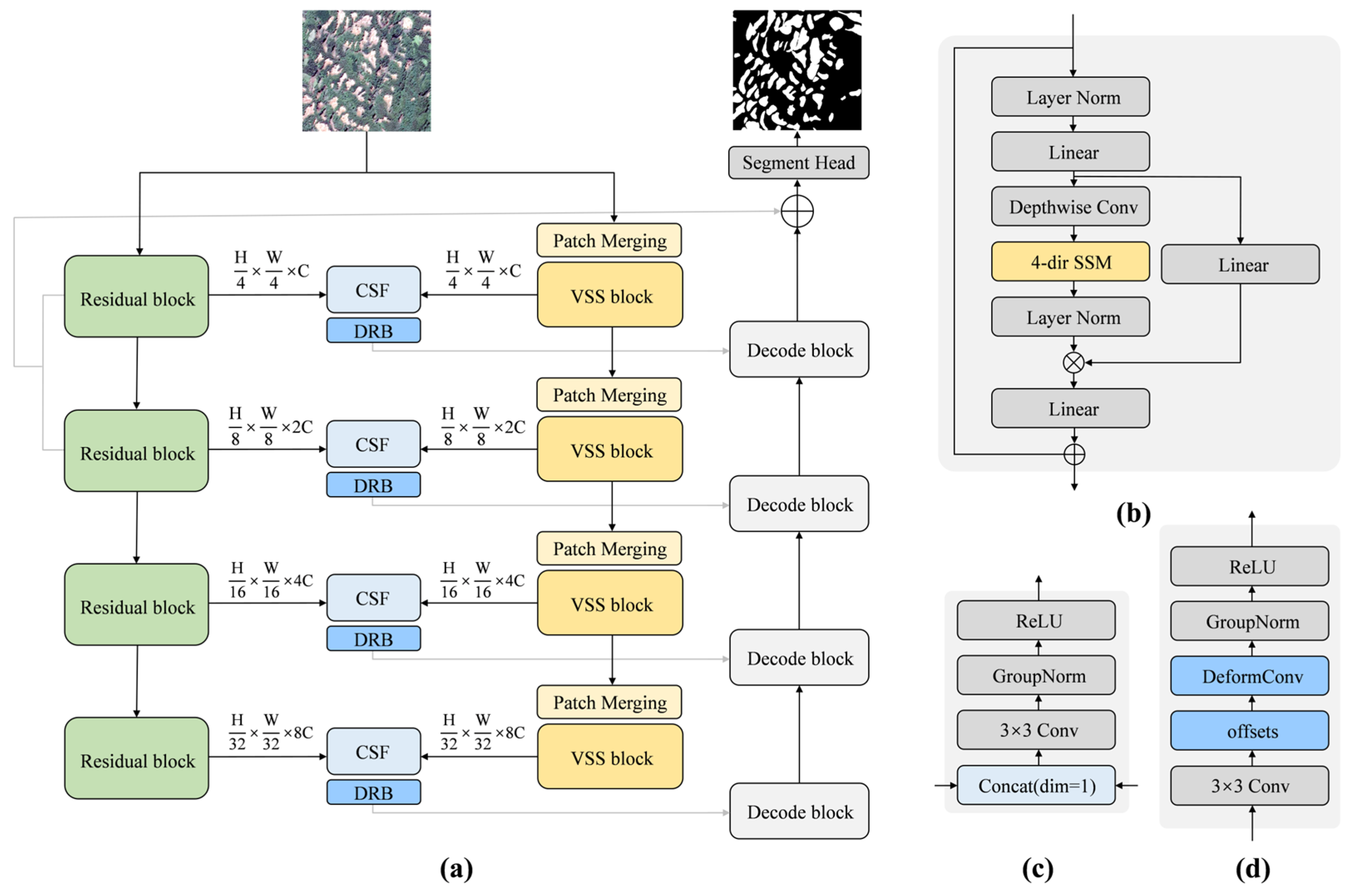
To adapt SSMs to vision tasks, we introduce a parallel VSSMEncoder branch to capture large-context representations from remote-sensing imagery. The VSSMEncoder is composed of stacked VSSBlocks, each including pre-normalization, a four-directional state-space modeling (4-dir SSM) module, and a residual connection (
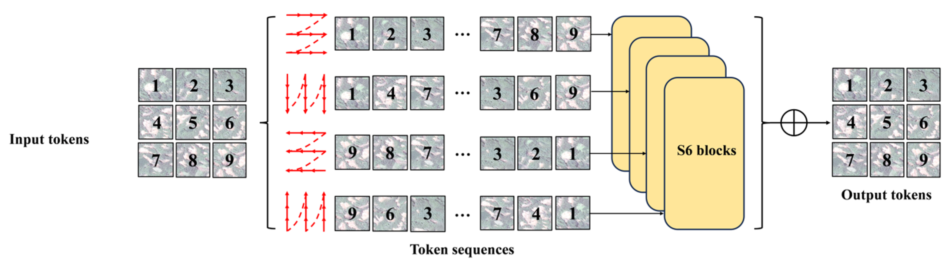
Figure 1b). Specifically, given an input feature map, channels are first expanded and processed by a depthwise convolution to inject local inductive bias. Next, a four-directional selective scan is performed along the horizontal and vertical axes and their reverse directions, producing four directional feature representations (
Figure 2). These directional outputs are then merged (by summation), followed by normalization and a gating mechanism that modulates the fused features, which are finally projected back to the original channel dimension.
This 4-dir SSM design is intended to provide two practical benefits for large-scene segmentation. First, the computational and memory complexity scales approximately linearly with the sequence length, which avoids explicitly constructing dense attention matrices and is therefore compatible with large-resolution tiled processing. Second, scanning along both axes in forward and reverse directions enables information propagation across the entire feature map, which is designed to support global semantic interaction beyond local windows and to mitigate discontinuities that may arise in patch-wise inference.
2.2. Cross-Scale Fusion (CSF)
To couple the local semantic features from the convolutional branch with the global contextual features produced by the VSSMEncoder branch [
32], we design a Cross-Scale Fusion (CSF) module that performs explicit alignment and fusion at multiple scales (
Figure 1c). Specifically, at each scale level
, we take the ResNet feature
and the VSSM feature
. The VSSM feature is first projected to a matched channel dimension and spatially aligned to
via bilinear interpolation. The aligned features are then concatenated along the channel dimension and processed by a
convolution followed by GroupNorm and ReLU for channel mixing and compression, yielding the fused feature
:
where [
] denotes channel-wise concatenation,
is the channel-projected and spatially aligned VSSM feature,
is GroupNorm, and
is the ReLU activation.
This fusion strategy is designed to reconcile feature discrepancies across branches (e.g., resolution and channel statistics) through an explicit alignment–interaction pathway, rather than directly combining features by element-wise addition. By performing fusion stage-by-stage across multiple scales, CSF facilitates information exchange between shallow texture/boundary cues and deeper semantic/contextual representations within a unified feature space. In addition, GroupNorm is adopted to reduce sensitivity to batch size and to stabilize optimization when fusing features with different distributions. Overall, CSF serves as a lightweight mechanism to support local–global collaboration and multi-scale consistency in large-scene landslide segmentation under tiled processing.
2.3. Deformable Residual Block (DRB)
To enhance geometry-adaptive refinement for irregular landslide boundaries and small targets, we attach a Deformable Residual Block (DRB) after the fused features at each scale [
33], as illustrated in
Figure 1d. In a standard 2D convolution, a regular sampling grid
is used to sample the input feature map. For an output location
on the feature map
, the convolution is computed as follows:
where
denotes the sampling offsets in the convolution kernel and
is the corresponding weight.
Deformable convolution introduces learnable offsets
to adapt the sampling locations from the regular grid points
to irregular positions
, leading to the following:
Because
is generally fractional, the feature value at the sampled position is obtained by bilinear interpolation:
where
,
traverses integer coordinates on the input feature map, and the interpolation kernel
can be decomposed as follows:
This interpolation is non-zero only at the four neighboring integer locations around , maintaining computational efficiency.
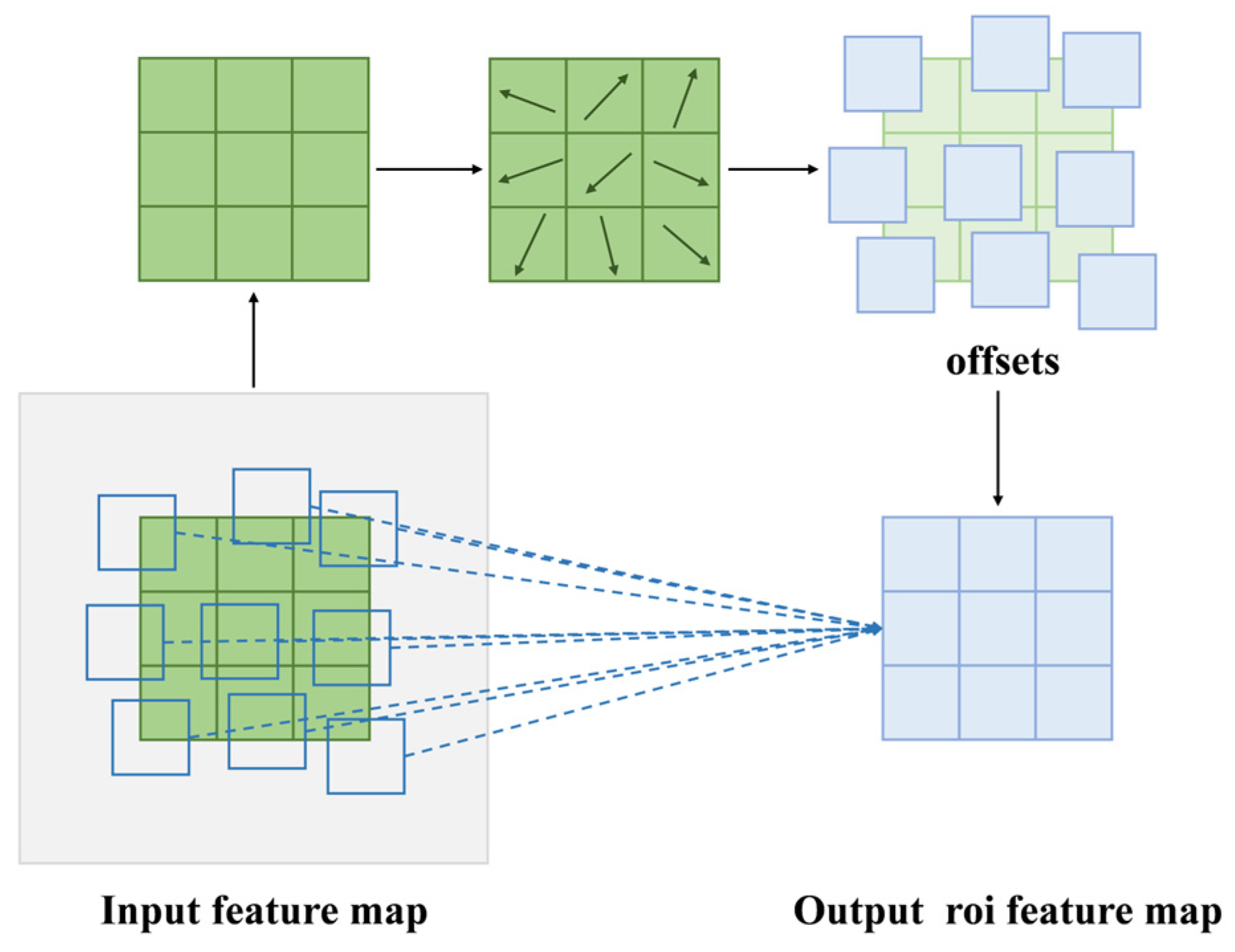
Implementation of DRB: In our DRB, a
convolution predicts the offset field
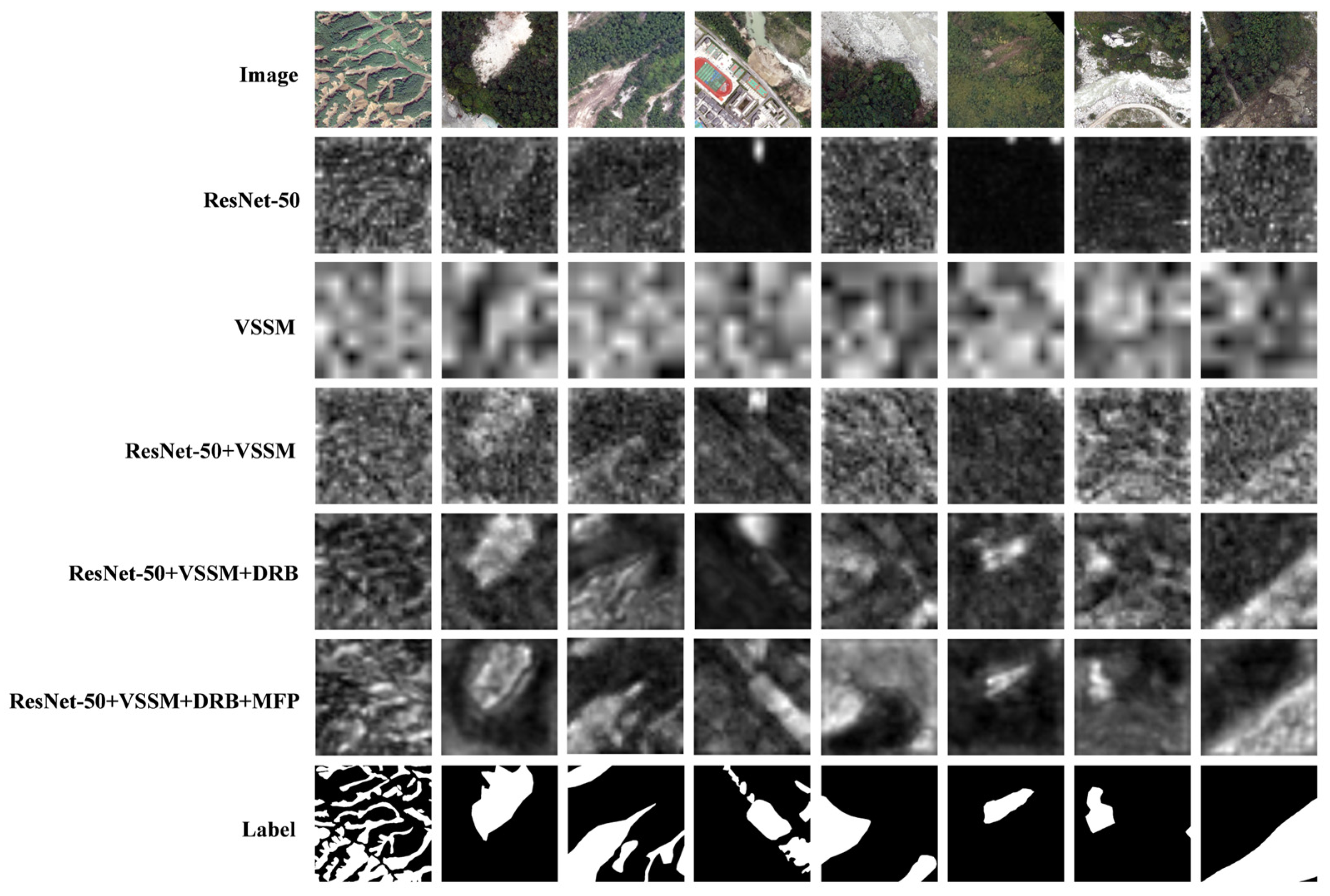
from the input features, followed by a deformable convolution for geometry-adaptive sampling. The output is further processed by GroupNorm and ReLU and combined in a residual manner to refine the fused representation (
Figure 3). To promote stable optimization, the offset prediction branch is initialized to produce near-zero offsets at the beginning of training, so the block starts from regular sampling and progressively learns geometry-adaptive adjustments. Overall, DRB is designed to provide boundary-aware refinement under multi-scale decoding, enabling the network to better adapt to jagged, tortuous contours and slender structures commonly observed in landslide regions.
2.4. Data Source
This study adopts the CAS Landslide Dataset, a recently released large-scale multi-sensor benchmark designed for deep-learning-based landslide recognition [
34]. The dataset contains 20,865 RGB remote-sensing images with pixel-level annotations, covering nine geographic regions and integrating multi-source data from both UAV (unmanned aerial vehicle) and SAT (satellite) imagery. All images are provided as 512 × 512 TIFF tiles, where landslide and non-landslide pixels are labeled as 1 and 0, respectively [
32].
The dataset is constructed following a quality-control workflow, including multi-source image acquisition, expert-assisted annotation, and combined automated/manual screening [
34]. Images with large blank areas, extremely low proportions of landslide pixels, severe cloud cover, or obvious stitching seams are excluded by the dataset provider.
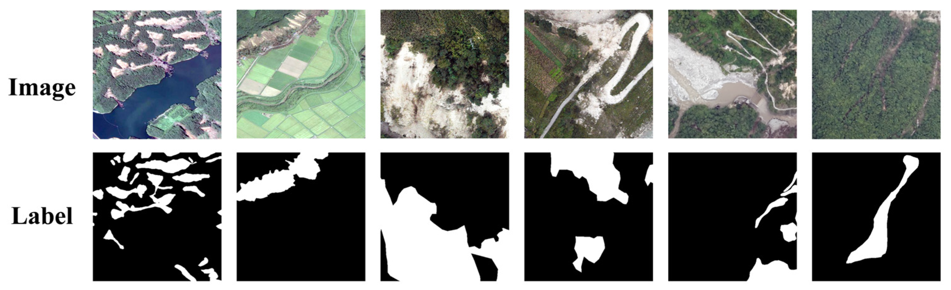
Figure 4 shows representative examples (UAV imagery and corresponding landslide masks), illustrating that landslides in this benchmark vary substantially in spatial distribution, morphology, and scale, and that complex backgrounds and topographic relief further increase the difficulty of precise delineation.
Data usage and splits: For the in-domain experiments, we select three representative subsets from the CAS Landslide Dataset to build the training/validation sets: Hokkaido Iburi-Tobu (SAT, 3.0 m), Moxi town (UAV, 0.2 m), and Moxitaidi (UAV, 0.6 m). These regions cover diverse geomorphological conditions and landslide-triggering mechanisms:
Hokkaido Iburi-Tobu (Japan, SAT 3.0 m): dominated by earthquake-induced landslides, spanning mountains, plateaus, and coastal plains. High vegetation coverage and steep slopes yield large deposits with clear but irregular boundaries.
Moxi town (Luding County, Sichuan, China, UAV 0.2 m): a high-mountain canyon region where rainfall-induced shallow landslides are common. Landslides are often irregular, numerous, and spatially scattered, posing challenges for small-object delineation and boundary transitions.
Moxitaidi (near Moxi Town, Sichuan, China, UAV 0.6 m): a high terrace in the Dadu River Basin (approximately 1600–2000 m elevation), surrounded by steep slopes. This area is influenced by tectonic activity near the Kangding–Luding seismic zone, where landslides can be triggered by earthquakes, heavy rainfall, and seasonal freeze–thaw cycles. Both deep-seated landslides and dense shallow failures occur, and diverse landforms (terraces, gullies, grass slopes, sparse forests) introduce complex visual patterns.
To improve training efficiency and mitigate extreme class imbalance, we filter out tiles with extremely small landslide areas (landslide pixel ratio < 1%) from the selected in-domain subsets. This results in 1000 in-domain samples used for model development, which are then split into training/validation/testing sets with an 8:1:1 ratio (i.e., 800/100/100).
Cross-domain test sets: To assess generalization beyond the in-domain distribution, we additionally evaluate the trained model on two independent cross-domain subsets, which are not used for training or validation:
Jiuzhai Valley (UAV, 0.2 m): a seismically induced landslide-prone area characterized by distinctive lithology (e.g., limestone and dolomite), high-altitude canyon landforms, and a subalpine climate. Vegetation is dominated by alpine coniferous forests and shrubs, resulting in image appearances that differ from the in-domain subsets.
Bijie (SAT, 0.8 m): a mountainous karst-affected region in southwest China with strong terrain relief and heterogeneous land cover. Compared with the in-domain subsets, Bijie exhibits different sensor characteristics and background textures (e.g., exposed rock, cultivated slopes, and patchy vegetation), providing an additional setting to examine cross-domain behavior under distinct resolution and imaging conditions.
For cross-domain evaluation, we use 200 tiles for Jiuzhai Valley and 200 tiles for Bijie as independent test sets. For completeness,
Table 1 also reports the positive-to-negative pixel ratios for these cross-domain subsets using the same statistical protocol, facilitating a consistent comparison of class imbalance across regions.
Overall, the configuration above supports both in-domain training/validation/testing and cross-domain testing, enabling evaluation of model performance across diverse geomorphological settings, triggering factors, and sensor conditions.