Combining Large Language Models with Satellite Embedding to Comprehensively Evaluate the Tibetan Plateau’s Ecological Quality

Highlights

What are the main findings?

• A new framework that combines large language models with satellite embeddings provides a comprehensive ecological assessment of the Tibetan Plateau from 2000 to 2024.
• The ESE-12 model exhibits high prediction accuracy for crucial ecological indicators (FAPAR R² = 0.9923; AGB R² = 0.8690) validated against field observations.

What are the implications of the main findings?

• This transferable approach addresses the limitations of single-source remote sensing by integrating multi-source data without task-specific calibration for high-altitude regions.
• The interpretable CRF framework enables practical decision-making by identifying three management zones: potential risk areas, enhancement potential areas, and stable conservation areas.

Abstract

As an important ecological obstacle prone to climatic changes, the Tibetan Plateau has been transformed by retreating glaciers, degrading permafrost, and deteriorating grasslands. Recent ecological remote sensing evaluations typically use medium-resolution and single-source optical imagery, highlight natural factors while ignoring human impacts, and encounter difficulties with time-focused interpretability and continuity within complex terrains. This research proposes a theory combining large language models with satellite embedding to holistically examine the ecology of the Tibetan Plateau between 2000 and 2024. We created an ecological satellite embedding (ESE) model applying self-supervised learning to integrate 12 ecological variables into combined space and time representations as of 2024, according to the Prithvi-Earth Observation (Prithvi-EO) foundational model involving low-rank adaptation (LoRA). GeoChat reasoning was applied to turn the embedded variables into a comprehensive representation feature (CRF). Field research demonstrated strong accuracy for the fraction of absorbed photosynthetically active radiation (FAPAR, R² = 0.9923) and aboveground biomass (AGB, R² = 0.8690). Space and temporal analyses demonstrated a general ecology-dependent enhancement accompanied by significant space-based clustering (Moran’s I = 0.50–0.80), hotspots in humid southeastern areas, major upward trends in vegetation indices and productivity metrics (p < 0.05), and higher shifts in transition regions. Despite the marginal degradation risk, the grassland carrying capacity has expanded extensively in the main farming regions. The comprehensible CRF schema identified three management areas: potential risk, enhancement potential, and stable conservation management. This transferable modular approach connects expert reasoning with data-driven modeling, presenting adaptable methods for assessing ecosystems in high-altitude, data-sparse environments, and practical ways to promote ecological management.

1. Introduction

The Tibetan Plateau, known as ‘Asia’s Water Tower’ and the ‘Roof of the World’ [1,2], is important due to its extreme sensitivity to a changing climate and its status as a necessary ecological obstacle [3]. In recent years, human actions and a warming planet have caused unprecedented and rapid regional shifts [4,5,6,7,8]. This is apparent in the quickened reduction in glacial fields, continuing degradation of permafrost, persistent deterioration of grassland, and heightened risk of loss of biological diversity. These shifts pose a threat to the local ecological conditions and ways of life of herders and also threaten major global and regional ecology by impacting patterns of atmospheric circulation as well as hydrological processes [9]. On the Tibetan Plateau, a region characterized by unique ecological conditions, ecosystems are subjected to the combined pressures of climate change and human activity, resulting in complex and dynamic variations in ecological functions and ecosystem conditions. In this study, ecological quality was defined as an integrated measure of ecosystem health and productivity, quantified using a set of key ecological indicators, including vegetation coverage, aboveground biomass, and grassland carrying capacity. This research primarily aims to assess these ecological function indicators and their long-term dynamics, with particular emphasis on evaluating ecosystem productivity and the potential for ecological recovery.

Remote sensing is necessary for observing the ecological status of plateaus due to its wide range, regular updates, and economic value. Ecological indices originating from this technology present a holistic method for measuring ecological status based on existing variables [10]. However, previous methods mostly relied on low- to medium-resolution imagery, including MODIS and Landsat, which cannot readily depict rapid shifts and fine-scale ecological differences in the complicated geography of the plateau, which is frequently covered by clouds. Within the past several years, assessments of habitat quality have become relevant for research on ecosystem services, offering a comprehensive view by incorporating landscape connectivity, threats to biodiversity, and shifting land use. Tools such as the InVEST model [11] have shown how human actions can drastically reduce the habitat quality of the Tibetan Plateau [12,13]. However, these methods are heavily reliant on expert parameterization and accurate land-use classification, causing considerable uncertainty in uninhabited high-altitude regions with limited data. A key challenge of many existing studies lies in their predominant reliance on natural–ecological indicators, such as land surface temperature and vegetation cover, with anthropogenic aspects of ecosystem change being inadequately represented. On the Qinghai–Tibet Plateau, pastoralism is the major way in which humans interact with the environment, and human impacts are expressed mostly through grazing pressure, livestock management, and rangeland use patterns, instead of typical indicators linked to urbanization or industrialization [14,15]. Because human–nature interactions are represented incompletely, it becomes harder to identify the fundamental drivers of changes in ecological quality.

Rapidly advancing artificial intelligence (AI) and the increase in sets of geography and geospatial data have highlighted the role of geography and space-based AI (GeoAI) [16,17], drastically changing ecological characterization and monitoring methods [18]. By combining AI, high-performance computing, and big data related to geography and space, GeoAI can systematically handle diverse and vast datasets that exceed the competencies of previous methods. This increases the reliability and accuracy of ecosystem monitoring using space-based modeling [19]. However, recent ecological evaluations of the Tibetan Plateau frequently rely on individual sources of data, such as MODIS or Landsat, as well as single model frameworks, limiting their capacity to portray the spatiotemporal relationships and spatial heterogeneity of the plateau’s complicated geography. Recently, improved multisource satellite remote sensing technology has drastically enhanced the collective observation capacity, including multispectral and hyperspectral sensors, synthetic aperture radar (SAR), and high-resolution optical imagery, presenting unique opportunities for developing terrestrial observations in multiple dimensions [20,21].

Satellite embedding has become essential for remote sensing models, altering the utilization of data related to Earth observations. Previous research has applied contrastive learning to connect coordinates to satellite images. For example, satellite contrastive language-image pre-training (SatCLIP) models use sinusoidal representation networks and spherical harmonic functions to encode global positions [22]. The model successfully transferred information across different geographic areas using zero- and few-shot learning functions. Embedding models have been gradually developed, including multiple sources of Earth observation data. AlphaEarth Foundation is a model that incorporates 10 heterogeneous data types, including light detection and ranging (LiDAR), radar, and optical data, and applies an architecture based on space, time, and precision [23]. This integration contributed to highly precise global mapping over continuous time scales, decreasing the error rates by over 23.9% for 15 downstream tasks. However, these models require improvements in computational efficiency, reproducibility, and transparency. The temporal embeddings of the surface spectra for earth representation and analysis (TESSERA) model addresses these problems by introducing a d-pixel representation that retains pixel-level time-series elements. Its dual-encoder architecture integrates Sentinel-2 multispectral data and Sentinel-1 SAR, creating concise 128-dimensional embeddings with a 24× compression ratio [24]. This forms a realistic embeddings-as-data structure, attaining or exceeding high-performance standards in ecological monitoring tasks, such as burn scar detection, aboveground biomass (AGB) retrieval, canopy height estimation, and crop classification.

Large language models (LLMs) are drastically changing geography and spatial analysis as a subversive AI technology. Current research has shown that these types of models, even when trained only on textual data, create linearized space- and time-related global models within neural networks [25]. This opposes the typical argument that LLMs only master statistical formats and make it possible to transfer geographic information from widespread Internet data to areas without remote sensing data. A remarkable improvement is the geography and space-based LLM methodology [26], which creatively changes OpenStreetMap’s open mapping data into ordered geography-based cues, integrating directional-distance relationships and reverse-geocoded addresses to regional locations. By applying parameter-efficient fine-tuning approaches such as low-rank adaptation (LoRA), geography and space-based LLM have successfully acquired implicit world geography-based information from large-scale models, including GPT-3.5. This is especially important for the Tibetan Plateau, an essential world ecological obstacle with limited ground observation facilities (less than one for every 10 km²), mainly in low-altitude valleys. Although ground observations are not widespread, large language models have been pretrained on broad and diverse text sources. Through this pre-training, they can retain implicit knowledge about socio-ecological connections, including how pastoral activities in high-altitude areas relate to grassland ecosystem functions and the sustainability of pastoral livelihoods. When added to multi-scale satellite-oriented phenology-linked observations, the combination of satellite data and LLMs shows potential for improving plateau ecological evaluations. This allows for a data-scarce, efficient, and cost-effective evaluation of the complicated interplay between society and nature on this plateau, presenting beneficial plans that integrate scientific disciplines with humanistic values for evaluating ecological security in the third pole.

This research proposes an ecological characterization structure for the Tibetan Plateau by combining satellite embedding methods with the rational capacity of LLMs. To tackle the recent difficulties in attaining a uniform space and temporal representation, as well as building comprehensive and interpretable indexes, we offer a two-stage workflow that guarantees interannual comparability, overall regional coverage, and interpretation-oriented outputs. During the initial stage, we implemented a satellite embedding–time series completion approach to combine 12 ecological variables, forming a yearly embedding set of data for 2000–2019. By combining these embedding models with Prithvi-Earth observations (Prithvi-EO) for stitching and temporal prediction, we expanded the series to 2020–2024 within one evaluation structure, creating a reliable and basic representation for the period 2000–2024. In the subsequent stage, we propose an interpretation-centered, reasoning-oriented, and overall representation approach using a grounded large-vision language model for remote sensing (GeoChat). Complying with explicit ecological logic, we created a comprehensive representation feature (CRF): the first 12 dimensions maintained the semantics of the initial variables, whereas the other linked dimensions involved enriched, standardized, and traceable descriptions across several ecological dimensions.

2. Study Area and Data Collection

2.1. Study Area

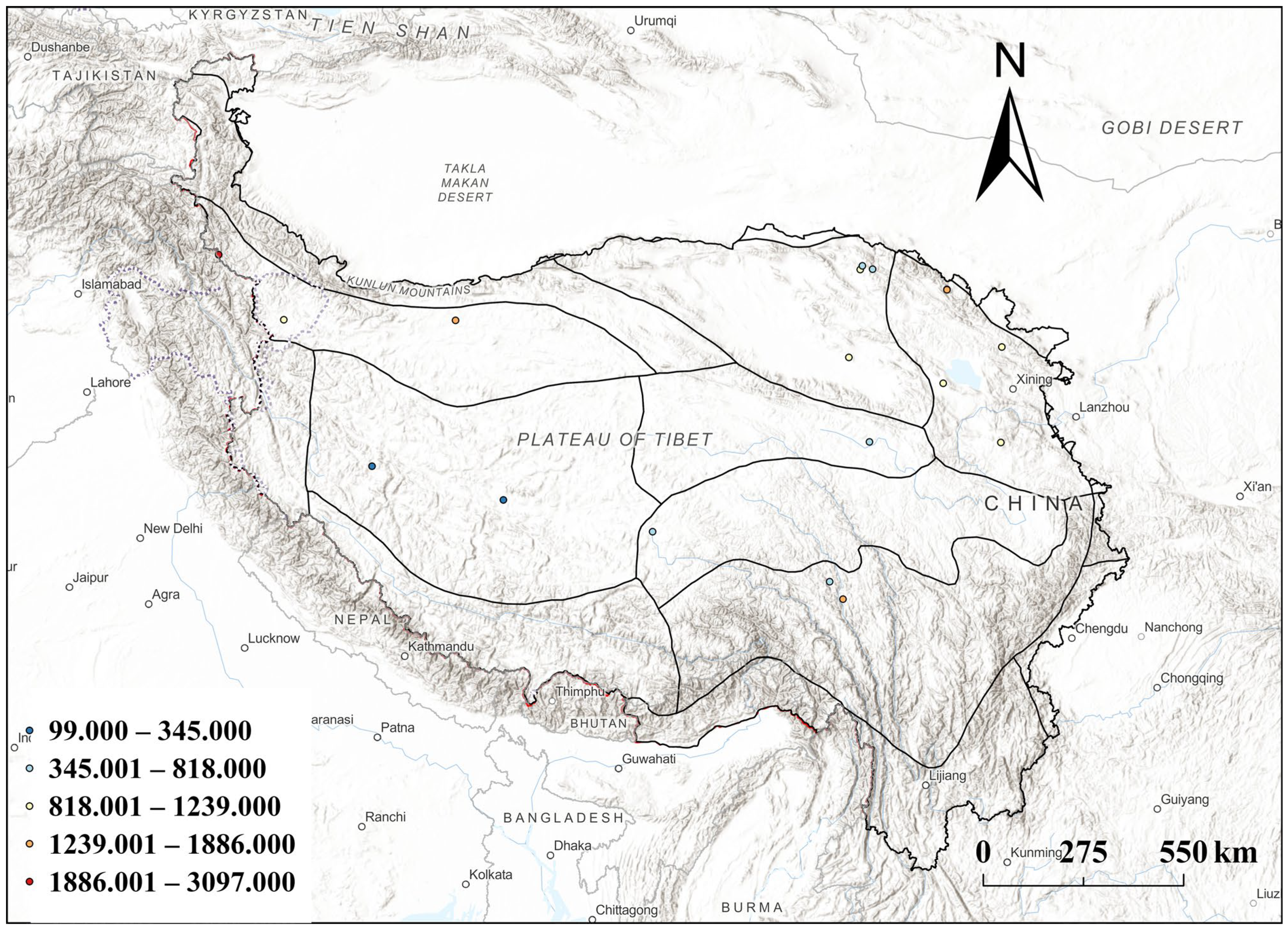
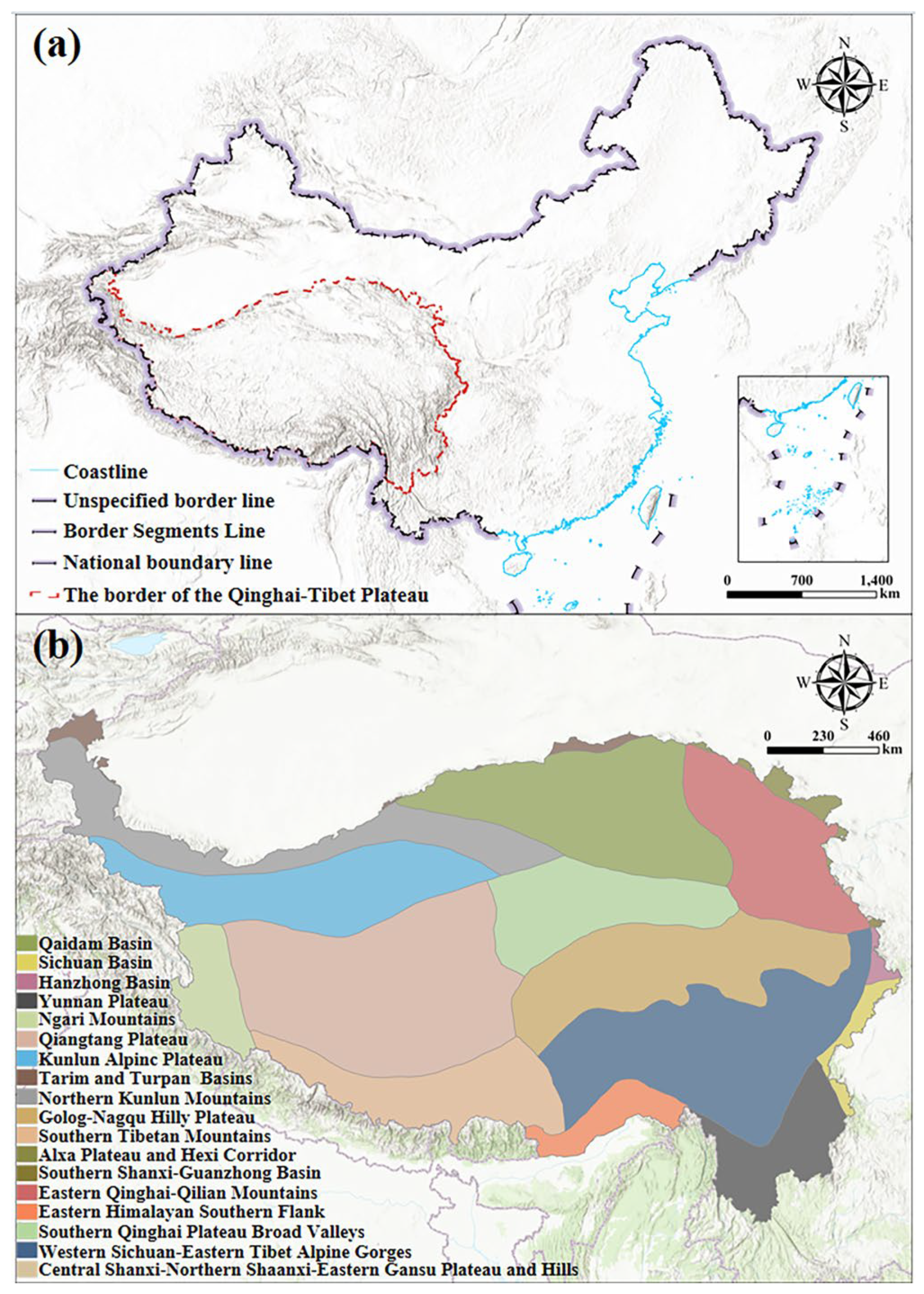
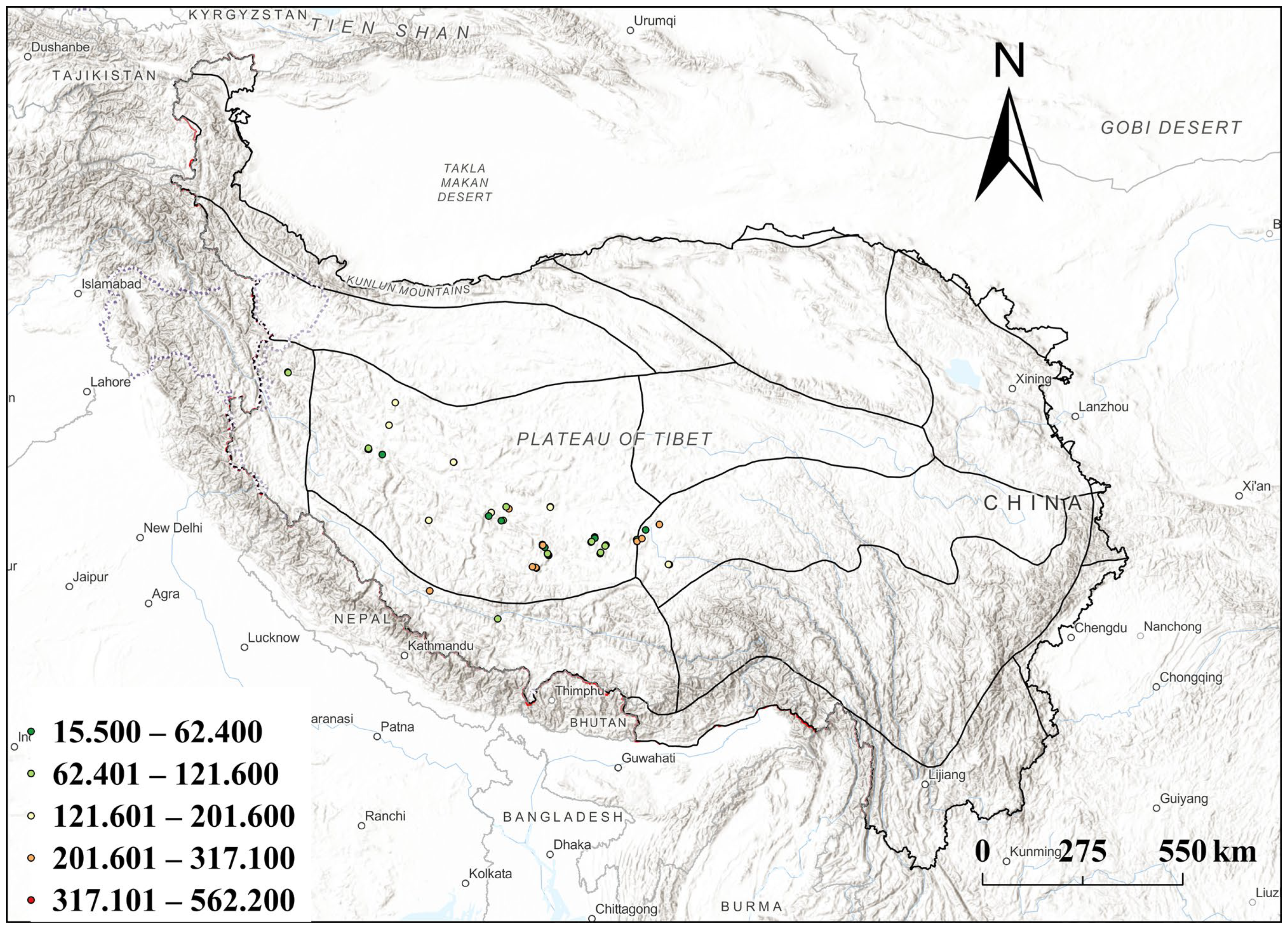
The Tibetan Plateau, located in western China between 73°18′52″–104°46′59″E and 26°00′12″–39°46′50″N, extends from the Pamir Plateau (west) to the Hengduan Mountains (east) (Figure 1). It is bordered by the Qilian, Altun, and Kunlun Mountains (north) and extends to the Himalayas (south), which is a crucial ecological security obstacle in China [27]. At elevations between 3000 and 5000 m, with an average of 4000 m, the plateau has wide-ranging climatic scenarios. These could be minimally accumulated or low temperatures, as well as highly variable precipitation and temperature distributions, which typify plateau climates [28]. This region supports numerous alpine ecosystems, including shrublands, alpine deserts, meadows, and steppes [29], making it necessary for overall biodiversity conservation and extremely sensitive to climate change. Known as Asia’s Water Tower, the Roof of the World, and the Third Pole, the Tibetan Plateau is among China’s most important sources of strategic resources [30].

Figure 1b illustrates the recent ecological and geographical regionalization of China, as argued by Wang et al. (2024) [31]. This separates the Tibetan Plateau into three areas: natural, moisture, and temperature zones. The major regions in arid areas are the Turpan, Tarim, and Qaidam Basins, Hexi Corridor, Alxa Plateau, Ngari and Northern Kunlun Mountains, and Kunlun Alpine Plateau. The semi-arid zones include the Eastern Qilian-Qinghai Mountains, Central Shanxi–Northern Shaanxi–Eastern Gansu Plateau and Hills, Qiangtang Plateau, Southern Qinghai Plateau Broad Valleys, and Southern Tibet Mountains. In semi-humid zones, the important areas are the Golog–Nagqu Hilly Plateau and the Southern Shanxi-Guanzhong Basin. The low-latitude, low-elevation, and humid zones include the Yunnan Plateau, Sichuan and Hanzhong Basins, Western Sichuan–Eastern Tibet Alpine Gorges, and Eastern Himalayan Southern Flank. This classification accurately describes the diverse ecology of the plateau, including arid, cold, and high-elevation deserts; montane forests; valley pastoral-agricultural ecotones; and alpine meadows. Future space and temporal interpretations and analyses using this structure guarantee consistency throughout the region and allow for correlations involving statistics-based results related to inherent ecological phenomena.

2.2. Data Collection and Data Sources

This research classified the data into three categories: background, ecological, and validation. Table 1 describes the time and space-based resolutions for the datasets. Background data includes position encoding and high-resolution surface qualities, highlighting China’s Landsat-originating annual land coverage product from the dataset of AlphaEarth Foundations embeddings [23] and Wuhan University [32].

Ecological data consists of indicators such as productivity, vegetation growth, and aspects of grasslands and forests, providing an overall awareness of ecological regional and grassland relationships. Vegetation indices, including the normalized difference vegetation index (NDVI) and enhanced vegetation index (EVI) at 250 m resolution, were obtained from MODIS products on the GEE platform. Productivity indicators, such as gross primary productivity (GPP) and net primary productivity (NPP), were evaluated at a 500 m resolution. Functional parameters of vegetation, such as evapotranspiration, tree coverage fraction (TreeCover), fraction of absorbed photosynthetically active radiation (FAPAR), and leaf area index (LAI) data at a 500 m resolution, were obtained from MODIS data using GEE. A grassland grazing intensity (GDGI) product [31] was used to assess the long-term impacts of human disturbance on grassland-based ecosystems. Biomass data from the National Tibetan Plateau Data Center included a reasonable livestock carrying capacity estimation product (RLCCEP) [33], grassland yield estimation product (GYEP) [34], edible pasture grass production (EPGP), and aboveground biomass (AGB) [35] at a space-based resolution of 250 m. To ensure that the datasets were comparable, all the raster layers were converted to a unified spatial resolution of 500 m. Datasets with finer resolution than the target (e.g., 250 m) were downsampled, whereas datasets with coarser resolution (e.g., 1000 m) were upsampled using suitable interpolation methods. After these steps, every dataset used for the analysis shared the same spatial resolution, providing a common spatial basis for inter-dataset comparison and integrated analysis.

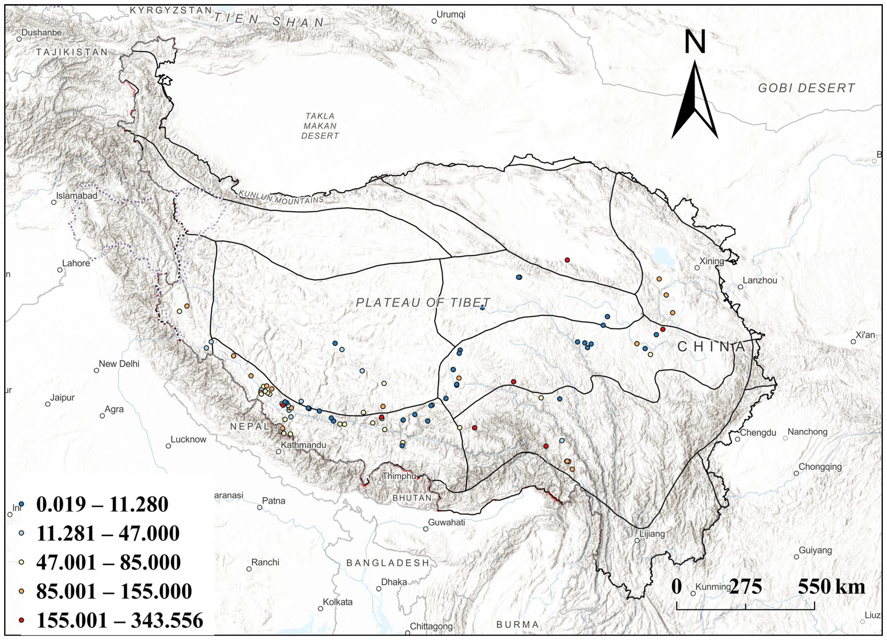
Validation data, which are generally based on ground-based measurements and field surveys, are essential for evaluating the accuracy and reliability of ecological products and model outputs. This includes survey data on grassland soil carbon storage [36], vegetation, soil plot survey data on AGB [37], vegetation investigation dataset, and spectral observation dataset [38]. To ensure that the validation data remained representative of the complex underlying surface conditions of the Tibetan Plateau, the spatial distribution of the in situ sampling sites was considered systematically. The sites were arranged across different parts of the plateau to cover a wide range of ecological conditions, including grasslands, alpine meadows, and forests. The sampling layout was designed to reflect the diversity of land cover types, topographic gradients, and climatic zones across the plateau. More details on the sampling sites are provided in Appendix A Figure A1, Figure A2 and Figure A3. Figure A1 illustrates the spatial distribution of soil carbon stock sampling sites, Figure A2 shows the locations of vegetation and soil plot surveys used for AGB measurements, and Figure A3 presents the distribution of vegetation surveys and spectral observation data points. Together, these figures indicate that the in situ sites are well representative across the ecological regions of the Tibetan Plateau, forming a solid basis for the comprehensive validation of model outputs.

Table 1. Data variables and sources.

Type	Spatial	Time	Sources	Website	Acquisition Date
Background Data	30 m	1984–2024	Yang and Huang, 2021 [32]	https://doi.org/10.5194/essd-13-3907-2021 (accessed on 26 November 2025)	2024
	10 m	2000–2025	AlphaEarth foundation embeddings dataset	https://data.tpdc.ac.cn/ (accessed on 26 November 2025)	2025
Ecological Data	250 m	2000–2024	MODIS-derived NDVI	https://developers.google.com/earth-engine/ (accessed on 26 November 2025)	2024
	500 m	2000–2020	MODIS-derived NPP	https://developers.google.com/earth-engine/ (accessed on 26 November 2025)	2020
	500 m	2000–2020	MODIS-derived GPP	https://developers.google.com/earth-engine/ (accessed on 26 November 2025)	2020
	250 m	2000–2019	Zhong and Wang, 2025 [35]	https://doi.org/10.11888/Terre.tpdc.302797 (accessed on 26 November 2025)	2025
	500 m	2002–2025	MODIS-derived LAI	https://developers.google.com/earth-engine/ (accessed on 26 November 2025)	2025
	250 m	2000–2024	MODIS-derived EVI	https://developers.google.com/earth-engine/ (accessed on 26 November 2025)	2024
	500 m	2000–2024	MODIS-derived FAPAR	https://developers.google.com/earth-engine/ (accessed on 26 November 2025)	2024
	500 m	2000–2024	Hansen Global Forest Change-derived TreeCover	https://data.tpdc.ac.cn/ (accessed on 26 November 2025)	2024
	250 m	2000–2019	Liu, 2021 [34]	https://doi.org/10.11888/Ecolo.tpdc.271514 (accessed on 26 November 2025)	2019
	250 m	2000–2019	Liu, 2021 [33]	https://doi.org/10.11888/Ecolo.tpdc.271515 (accessed on 26 November 2025)	2019
	250 m	2000–2019	EPGP	https://data.tpdc.ac.cn/ (accessed on 26 November 2025)	2019
	100 m	1980–2024	GDGI	https://data.tpdc.ac.cn/ (accessed on 26 November 2025)	2024
Validation Data	–	2005–2006	Hu, 2021 [36]	https://doi.org/10.11888/Terre.tpdc.300275 (accessed on 26 November 2025)	2006
	–	2019–2023	Xu et al., 2021 [37]	https://doi.org/10.11888/Terre.tpdc.271995 (accessed on 26 November 2025)	2021
	–	2020	Li, 2025 [38]	https://doi.org/10.6084/m9.figshare.27316002.v3 (accessed on 26 November 2025)	2024

Note: Units of ecological variables are as follows: NDVI and EVI (dimensionless); GPP and NPP (g C m⁻² yr⁻¹); AGB (g m⁻²); LAI (m² m⁻²); FAPAR (dimensionless); TreeCover (%); GYEP and EPGP (kg ha⁻¹); RLCCEP (sheep units ha⁻¹); and GDGI (dimensionless index). A dash (“–”) denotes point-based field measurements for which the spatial resolution is not applicable.

Table 1. Data variables and sources.

Type	Spatial	Time	Sources	Website	Acquisition Date
Background Data	30 m	1984–2024	Yang and Huang, 2021 [32]	https://doi.org/10.5194/essd-13-3907-2021 (accessed on 26 November 2025)	2024
	10 m	2000–2025	AlphaEarth foundation embeddings dataset	https://data.tpdc.ac.cn/ (accessed on 26 November 2025)	2025
Ecological Data	250 m	2000–2024	MODIS-derived NDVI	https://developers.google.com/earth-engine/ (accessed on 26 November 2025)	2024
	500 m	2000–2020	MODIS-derived NPP	https://developers.google.com/earth-engine/ (accessed on 26 November 2025)	2020
	500 m	2000–2020	MODIS-derived GPP	https://developers.google.com/earth-engine/ (accessed on 26 November 2025)	2020
	250 m	2000–2019	Zhong and Wang, 2025 [35]	https://doi.org/10.11888/Terre.tpdc.302797 (accessed on 26 November 2025)	2025
	500 m	2002–2025	MODIS-derived LAI	https://developers.google.com/earth-engine/ (accessed on 26 November 2025)	2025
	250 m	2000–2024	MODIS-derived EVI	https://developers.google.com/earth-engine/ (accessed on 26 November 2025)	2024
	500 m	2000–2024	MODIS-derived FAPAR	https://developers.google.com/earth-engine/ (accessed on 26 November 2025)	2024
	500 m	2000–2024	Hansen Global Forest Change-derived TreeCover	https://data.tpdc.ac.cn/ (accessed on 26 November 2025)	2024
	250 m	2000–2019	Liu, 2021 [34]	https://doi.org/10.11888/Ecolo.tpdc.271514 (accessed on 26 November 2025)	2019
	250 m	2000–2019	Liu, 2021 [33]	https://doi.org/10.11888/Ecolo.tpdc.271515 (accessed on 26 November 2025)	2019
	250 m	2000–2019	EPGP	https://data.tpdc.ac.cn/ (accessed on 26 November 2025)	2019
	100 m	1980–2024	GDGI	https://data.tpdc.ac.cn/ (accessed on 26 November 2025)	2024
Validation Data	–	2005–2006	Hu, 2021 [36]	https://doi.org/10.11888/Terre.tpdc.300275 (accessed on 26 November 2025)	2006
	–	2019–2023	Xu et al., 2021 [37]	https://doi.org/10.11888/Terre.tpdc.271995 (accessed on 26 November 2025)	2021
	–	2020	Li, 2025 [38]	https://doi.org/10.6084/m9.figshare.27316002.v3 (accessed on 26 November 2025)	2024

Note: Units of ecological variables are as follows: NDVI and EVI (dimensionless); GPP and NPP (g C m⁻² yr⁻¹); AGB (g m⁻²); LAI (m² m⁻²); FAPAR (dimensionless); TreeCover (%); GYEP and EPGP (kg ha⁻¹); RLCCEP (sheep units ha⁻¹); and GDGI (dimensionless index). A dash (“–”) denotes point-based field measurements for which the spatial resolution is not applicable.

2.3. Operationalization of the Human Dimension in Pastoral Ecosystems

In this study, the “human dimension” was represented using pastoral land-use indicators that fit the socio-ecological system context of the Qinghai–Tibet Plateau. Unlike traditional social indicators often used in lowland areas (e.g., urban infrastructure density and industrial output), human influence on the plateau is mainly expressed through the following: GDGI, which describes the spatiotemporal pattern of anthropogenic pressure from livestock grazing on grassland ecosystems; RLCCEP, which represents the sustainability threshold of ecosystem services under human use by combining limits from ecological productivity with the socioeconomic demands of livestock management; and EPGP, which indicates the capacity of ecosystems to provide forage resources for pastoral livelihoods by linking natural productivity with human subsistence needs. These variables capture the principal patterns of human–environment interaction in high-altitude pastoral areas, where natural grasslands cover more than 60% of the land area and pastoralism supports most residents. This selection also follows the idea of context-dependent socio-ecological indicators, meaning that measures of human influence should reflect dominant socioeconomic activities in a specific regional context.

3. Methods

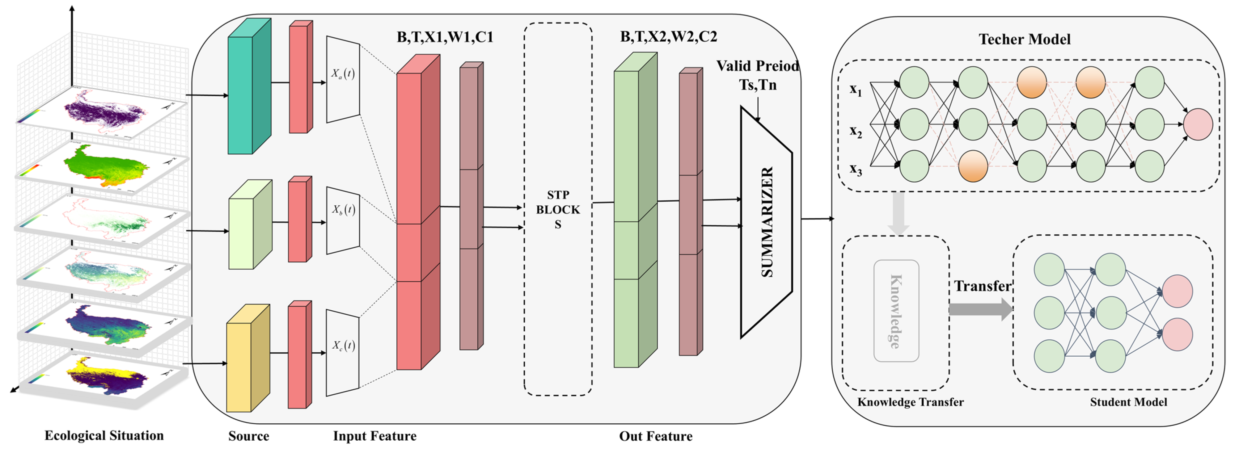
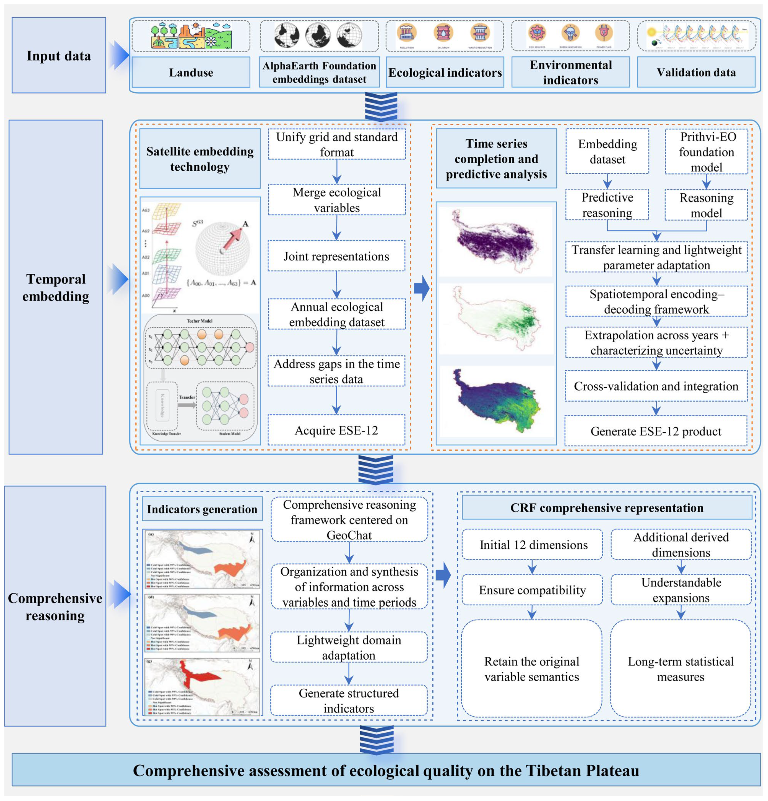
This study addresses a central scientific problem: the development of a comprehensive socio-ecological assessment of the Tibetan Plateau using remote sensing. Emphasis is placed on describing the dominant human–environment interaction on the plateau, namely pastoral land use, using grassland-related indicators [39,40]. To address this, we developed a two-stage structure called unified embedding–comprehensive reasoning (Figure 2). In the first stage, satellite embedding technology was used to integrate 12 ecological variables related to productivity (AGB, EVI, RLCCEP, EPGP, FAPAR, GDGI, GPP, GYEP, LAI, NDVI, NPP, and TreeCover) into a single grid with a standardized pattern. By learning joint representations across years and variables, we generated a yearly ecological embedding dataset, ESE-12, with pixel-level continuity for the period 2000–2019. We then filled the gaps in the time-series data from 2020 to 2024, establishing a standardized ESE-12 dataset covering 2000 to 2024. To address this, we applied two methods for time-series completion and predictive analysis of data gaps from 2020 to 2024. Firstly, the embedding model conducted a stable prediction. Secondly, Prithvi-EO was implemented for temporal multi-source remote sensing, including transfer learning as well as lightweight parameter adaptation, like LoRA. This created a space- and temporal decoding-encoding structure that contributed to the production of important variables over several years and portrayed uncertainty with quantile/ensemble-based confidence bounds. We cross-validated and integrated both methodologies with independent samples and ground quadratic data in an overall assessment structure, creating a standardized ESE-12 dataset for the years between 2000 and 2024.

In the subsequent phase, the ESE-12 model was improved by creating an overall reasoning structure based on GeoChat. This method arranges and combines information from multiple periods and variables. Based on lightweight domain adaptation, the representational ability of the model is maintained while producing organized indicating factors based on easily apparent ecological aspects. The CRF incorporates two primary elements: the initial 12 dimensions retain the semantics of the first variables to guarantee that they match the existing operational standards, and the extra related dimensions clearly expand the ecological conditions, as applied to multiple characteristics.

3.1. Ecological Satellite Embedding (ESE)

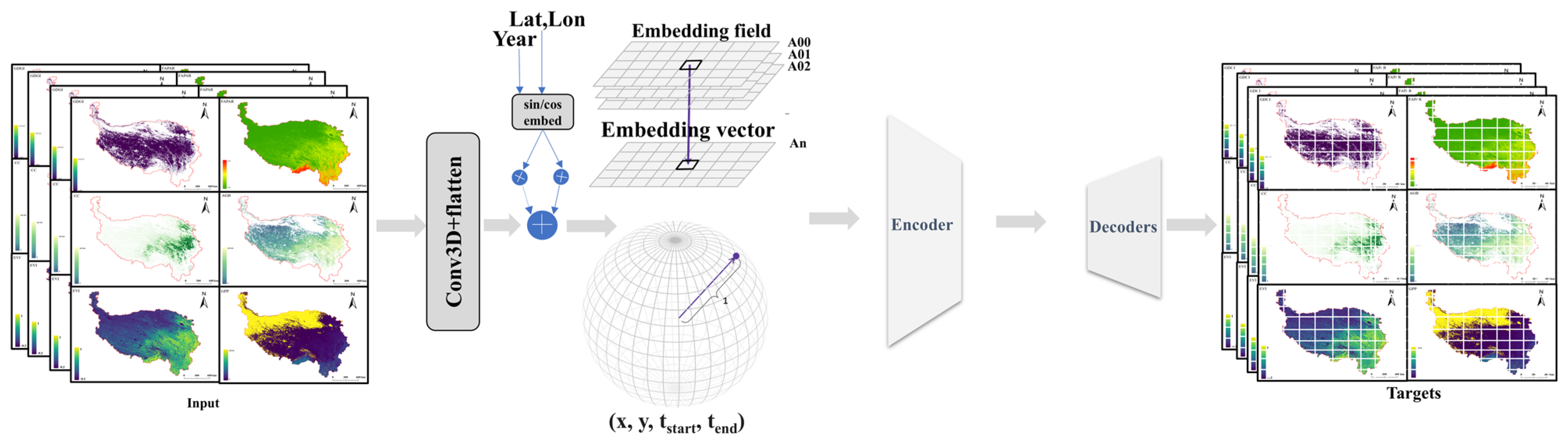
To create an enduring and cohesive portrayal of ecological data from remote sensing sources across the Tibetan Plateau, this study proposes an ESE model that implements self-supervised learning. The model design, as shown in Figure 3, originated from the constant space and temporal encoding methodology of the AlphaEarth Foundations model [23]. This builds a unitary representation integrating several modes and temporal dimensions, leading to a reduction in the volume of high-dimensional and ecological characteristics and incorporating them in a space and temporal scenario. Operating without specified task-focused limitations, the model identifies the inherent distribution-focused sequences of surface ecological processes from remote sensing data patterns that require processing. Consequently, it creates a field of vectors representing ecosystem states that demonstrate constant differentiation in time and space-based dimensions. An ecological observation with multiple sources is set at time point ${\mathrm{t}}_j$ identified as:

$$X\left(t\right)=\left[X_1\left(t\right),X_2\left(t\right),\dots ,X_M\left(t\right)\right]$$

(1)

where $X_i\left(t_j\right)$ is a representation of the space-based distribution qualities of the i-th ecological variable, and M represents the overall number of variables. Within a specified interval of time $\left(t_s,t_e\right)$, the ESE model maps the time series with multiple sources into the embedding area by using a parameterized mapping function to put this time series onto the embedding area:

$$z=f_e\left(x\left(t_g:t_e\right),m,t_s,t_e\right)$$

(2)

where $z\in R^d$ represents an ecological scenario embedding vector of length d, and m includes geographic and sensor metadata including latitude, climate zoning, longitude, and resolution. This combined vector embodies the overall ecological state and changing surface tendencies over the time period $\left(t_s,t_e\right)$, allowing for tasks linked to extrapolation and interpolation predictions.

3.1.1. Time and Space Encoding

The ESE model combines space-based trends and temporal processing interactions. To portray temporal stability, it proposes a sinus-shaped time-encoded function described as

$$\mathsf{\Phi }\left(t_i\right)=\left[\sin \left({\omega }_i{t}_i\right),\cos \left({\omega }_i{t}_i\right),\dots ,\sin \left({\omega }_k{t}_i\right),\cos \left({\omega }_k{t}_i\right)\right]$$

(3)

where ${\omega }_k$ embodies the k-th frequency aspect. Every input time period considers $\mathsf{\Phi }\left(t_j\right)$ as a conditioning signal, enabling the model to portray seasonal cycles and long-term variations. Space-based feature encoding applies an attention–convolution combined structure to simultaneously portray large-scale ecological patterns and local details. After traversing several space- and temporal encoding layers, the model generates the final representation of the embedding as follows:

$$h^{(l+1)}=ST{P}^{(l)}(h^{(l)},\varphi (t_j)),z={\mathit{Resample}(h}^{\left(L\right)})$$

(4)

where $h^{(l+1)}$ represents the hidden state tensor at layer $l$, while $ST{P}^{(l)}$ symbolizes the space-time precision block, which is composed of three operators: precision convolution, temporal attention, and space-based attention.

3.1.2. Self-Supervised Learning Objective

The ESE model implements a self-supervised training method in which the evolution of the embedding area is influenced by contrastive consistency loss and reconstruction loss. This intends to highlight stable representations throughout enhanced viewpoints. Reconstruction loss guarantees that the model restores the initial distribution of ecological variables, even with perturbed or masked inputs.

$${\xi }_{rec}={\displaystyle \frac{1}{\left|\mathsf{\Omega }\right|}}{{\displaystyle \sum _{(x,y)\in \mathsf{\Omega }}\left(X(z,y)-\widehat{X}(x,y)\right)}}^2$$

(5)

where Ω represents a valid pixel set. Contrastive loss strengthens the discriminative influence of the embedding area by limiting the similarities between the enhanced samples.

$${\xi }_{\mathrm{con}}=-{\displaystyle \frac{1}{B}}{\displaystyle \sum _{i=1}^B\log \frac{\exp (sim(q_i,k_i)/\tau )}{{\displaystyle {\sum }_{j=1}^B\exp (sim(q_i,k_i)/\tau )}}}$$

(6)

with $sim(\cdot )$ as the cosine similarity, τ as the temperature parameter, while $q_i,k_i$ embodies positive sample pair embedding. To promote a regularly distributed ecological representation on the unit hypersphere, a batch uniformity objective is shown as

$${\xi }_{uni}={\displaystyle \frac{1}{B^2}}{{\displaystyle \sum _{i\ne j}‖z_i^T{z}_j-{\tau }_0‖}}^2$$

(7)

By integrating these three goals, the comprehensive optimizing goal of our ESE model is described as

$${\xi }_{ESE}={\xi }_{rec}+{\lambda }_1{\xi }_{con}+{\lambda }_2{\xi }_{uni}$$

(8)

with ${\lambda }_1,{\lambda }_2$ denoting the balance coefficient. After this model is trained, it creates a vector field with 14 dimensions, described as $Z_t\in {ℝ}^{14*H*W}$, symbolizing the ecological scenario embedding for every period of time. This form of embedding has constant stability over the entire geographical area, contributing to temporal extrapolation and interpolation.

3.2. Large Language Model

This research proposed a detailed structure for enriching semantic knowledge and combined reason in ecological situations. This structure is based on various large-scale basic geographical models intended to analyze high-dimensional ESE outputs. Through semantic improvement with multiple sources and structured generation of knowledge, along with a cross-modal feature arrangement, this structure allows for hierarchy-based mapping, ranging from semantic interpretations to quantitative representations of situations. This research used two prominent large-scale pre-trained models to design the model: Prithvi-EO, a visual space and temporal joint encoding model intended for Earth observational data, and GeoChat, a multimodal model designed to promote geographical vision, language understanding, and interactions between AI and humans.

3.2.1. Prithvi-EO

Prithvi-EO is a prominent Earth observation model that uses temporal and multiple-source remote sensing data as its main input, implementing a space- and temporal transformer structure [41]. This structure is depicted in Figure 4 and is based on the concept of viewing surface remote sensing time series as complicated and high-dimensional dynamic systems. It depicts the cross-time dependencies and correlations among remote-sensing signals from several sources using a temporal self-attention mechanism. Given a time series of ecological variables $X={\left\{x_t\in {ℝ}^{C\times H\times W}\right\}}_{t=1}^T$, Prithvi-EO performs space and temporal embedding as follows:

$$Z_t=E_s(x_t)+E_t(t)+E_p(pos)$$

(9)

where E_s represents the space-based feature encoding, E_t represents the temporal position encoding, and E_p represents the geography-based position embedding. After passing through the multilayer self-attention modules, the model depicted long-term evolutionary tendencies, seasonal fluctuations, and multivariate coupling relationships.

Although Prithvi-EO was developed for general Earth observation tasks, it still requires focused adaptations to satisfy the needs of gap filling and prediction for plateau ecological time series. This is especially true in regions such as the Tibetan Plateau, where observations are sparse and the ecosystems are highly complex. Several key adaptations were implemented to render the model suitable for the tasks addressed in this study.

First, the model was adjusted to handle heterogeneous spatial resolutions in the input dataset. The ecological data used here included several variables with inconsistent spatial resolutions (100–500 m), such as NDVI, GPP, AGB, and TreeCover. To effectively integrate these multi-resolution inputs, a resolution-aware embedding head was added. Before the data entered the transformer encoder, this module projected all variables into a shared latent space, which allowed the model to process both coarse and high-resolution spatial signals and learn key interactions among different ecological variables.

Second, because missing values are widespread in ecological time-series datasets, the model uses a masked prediction objective inspired by masked language modeling. This design allows the model to reconstruct missing observations by drawing on historical records and other available ecological indicators. In this way, the model gains temporal reasoning ability and produces continuous and comparable embedding representations across years. This adaptation improves the robustness of ecological time-series gap filling and is well suited for missing data situations that result from sparse sampling over large spatial regions.

In addition, Prithvi-EO was adapted to learn jointly from multiple ecological indicators including productivity, structure, pressure, and management factors. Training was conducted with a multi-channel input tensor that contained these variables, enabling the self-attention mechanism to learn coupling relationships among indicators, such as the influence of grazing intensity on biomass and feedback from vegetation dynamics to carbon stocks. This joint learning strategy is important for characterizing coupled ecological processes because it allows interactions among different variables to be considered within a unified ecosystem framework.

During the inference stage, this research applied Prithvi-EO to the temporal completion and future prediction of ecological scenario embeddings, producing constant ecological state fields from 2000 to 2024 to dynamically support subsequent integrated representations. The prediction operator is described as

$${\widehat{x}}_{t+k}=f_{\theta }(X_{1:t}),k\in [1,K]$$

(10)

Based on the sequence of embedding in the past time period t, the model provides predictions about ecological changes in variables for subsequent K steps, contributing to temporal reasoning and forecasting of ecological situations.

3.2.2. GeoChat

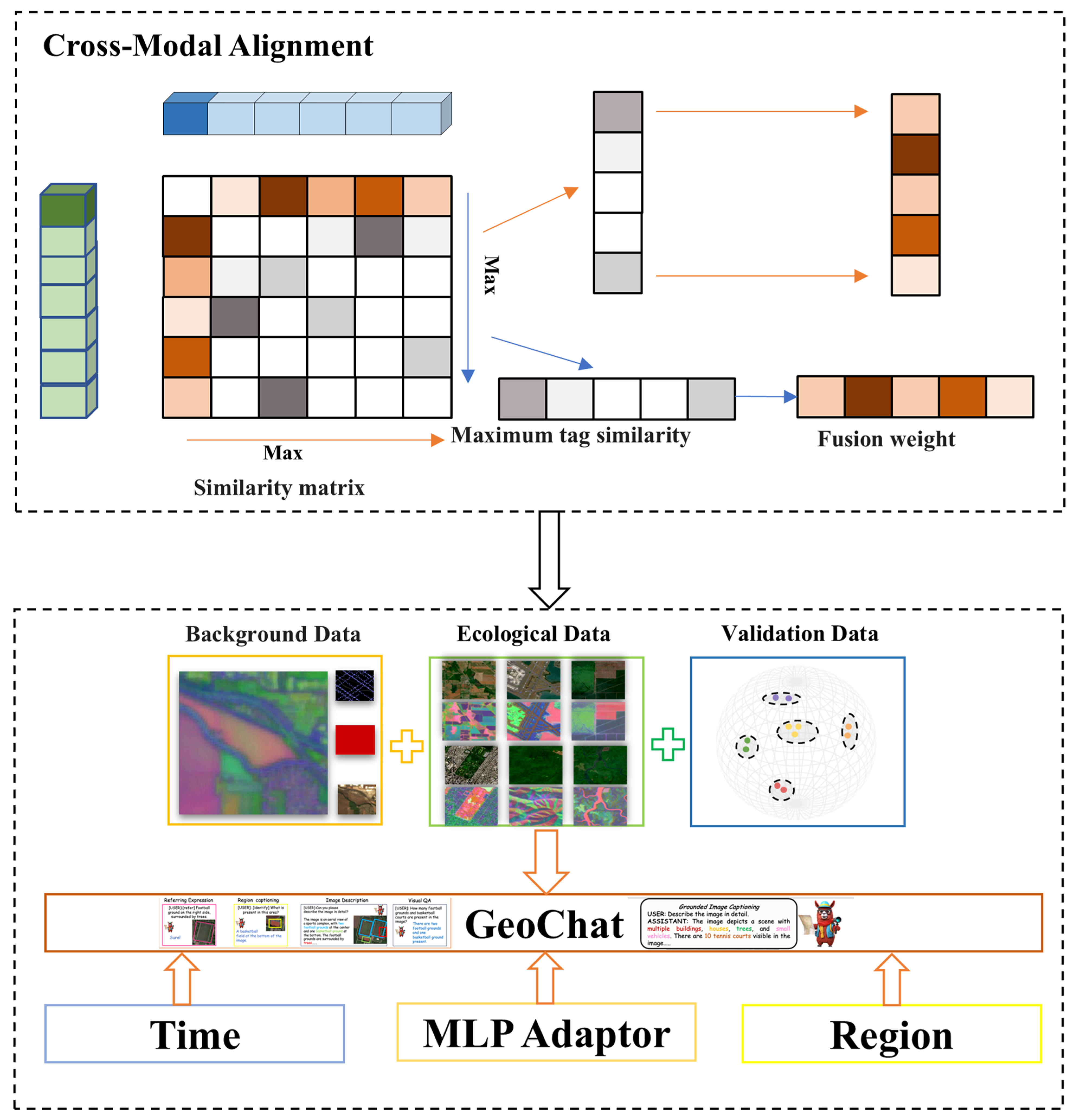
GeoChat is a special multiple-mode alignment model designed for geography-based tasks. It relies on a vision-language transformer structure and is trained through joint pre-training tasks that merge geography-based text with remote sensing imagery. This matches textual and visual semantics to increase geographical and space-based awareness [42]. The GeoChat structure, shown in Figure 5, emphasizes cross-modal alignment and space-based grounded textual understanding. The mapping function is expressed as follows:

$$h_{geo}=g_{\varphi }(\mathrm{I},\mathrm{T})$$

(11)

where I symbolizes the geography-based image input (or ecological embedding map) and T indicates a text-focused summary. GeoChat calculates the cross-modal contrastive loss in the collective latent representation area using language and a visual encoder as follows:

$${\xi }_{align}=-\log {\displaystyle \frac{\exp (sim(v_i,t_i)/\tau )}{{\displaystyle {\sum }_j\exp (sim(v_i,t_j)/\tau )}}}$$

(12)

After the LoRA fine-tuning was completed, the model acquired the capacity to comprehend, describe, and react to geography-based semantic queries. It can create natural language descriptions for anomalous areas, shifting situations, or certain patterns of variables within maps for embedding. In this research, GeoChat was used for tasks linked to the comprehension of space-based semantics and depictions of ecological changes, including the creation of regional ecological synopses, recognition of change patterns, and elucidation of processes for ecological evolution.

3.2.3. LoRA

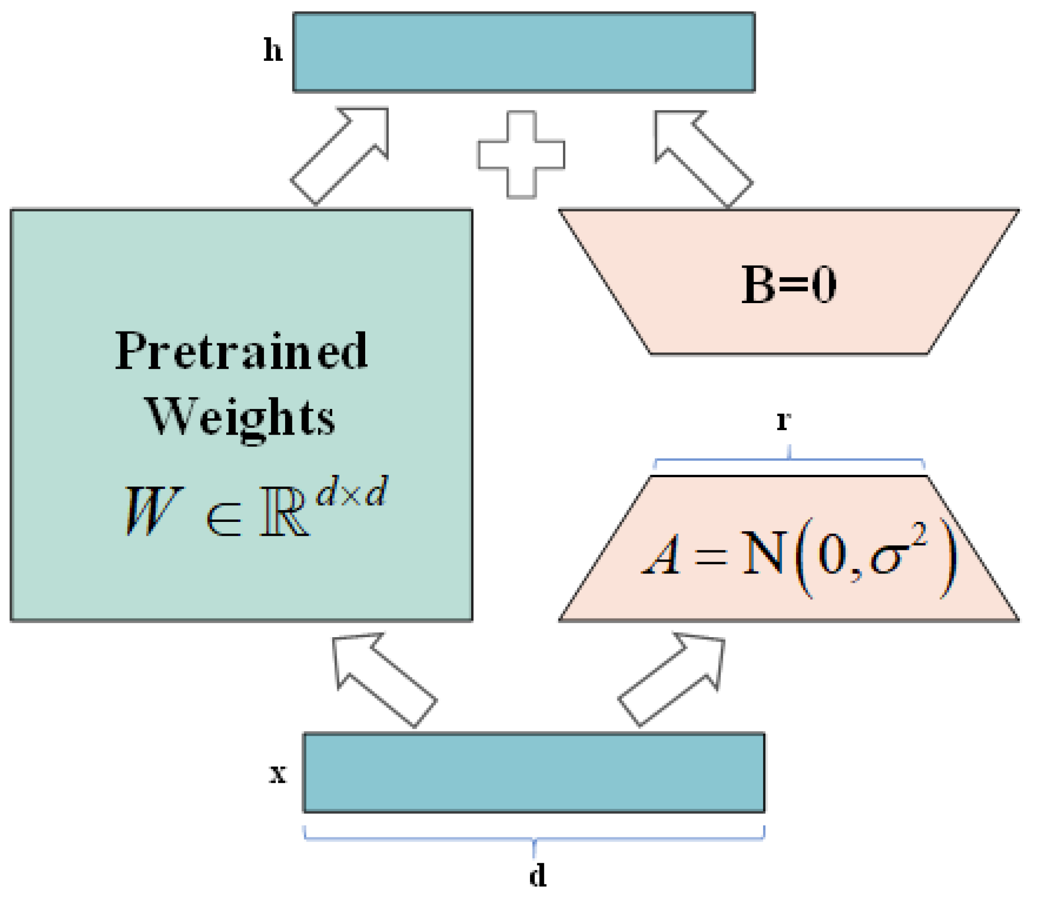
LoRA enables efficient fine-tuning of large models by applying low-rank factorization to linear transformations. The weights of the base model remain unchanged, and only a small set of low-rank parameters is updated, which significantly reduces the training cost and helps avoid catastrophic forgetting. In this study, LoRA was applied to adapt Prithvi-EO for ecological time-series tasks, with an emphasis on gap filling and prediction of ecological data on the Tibetan Plateau [43]. As illustrated in Figure 6, let denote the weight $W_0\in {ℝ}^{d_{ont}\times d_{in}}$ of a linear layer in the pre-trained model. Traditional full fine-tuning updates all elements of $W_0$, whereas LoRA introduces a learnable low-rank increment ΔW to approximate the parameter updates:

$$\begin{array}{l}W=W_0+△W\\ △W=BA\\ B\in {ℝ}^{d_{ont}\times r},A\in {ℝ}^{r\times d_{in}}\end{array}$$

(13)

During training, only $A,B,W_0$ was optimized, whereas the base weights remained frozen. To stabilize the training process, a scaling factor α is typically applied during the forward pass, as follows:

$$y=W_{0}x+{\displaystyle \frac{\alpha }{r}}BAx$$

(14)

where α controls the effective magnitude of the increment to prevent the low-rank update from introducing excessive perturbations into the base distribution, and because rank r (representing the rank of the low-rank decomposition) is small, both the number of new parameters and the memory overhead increase linearly with r. Compared with full fine-tuning, LoRA reduces the trainable parameters and communication costs by 10–100×.

For LoRA fine-tuning of Prithvi-EO, the hyperparameters were configured as follows: the rank $r$ of the low-rank decomposition was set to 8, providing a practical balance between model flexibility and parameter efficiency; a scaling factor of α = 0.1 was used during the forward pass to stabilize training; and the learning rate for LoRA parameters was set to 1 × 10⁻⁴, which is lower than the learning rate of the base model to avoid disrupting pretrained knowledge. These choices support efficient fine-tuning, allowing the model to adapt to the target ecological tasks while maintaining the generalization ability of the original model. Under these hyperparameter settings, Prithvi-EO can address the particular challenges of ecological time-series data on the Tibetan Plateau, achieving accurate prediction and gap-filling without full retraining of the model.

3.2.4. Accuracy Evaluation Metrics

To quantitatively assess the model’s predictive performance, this research applied three metrics: the coefficient of determination (R²), root mean square error (RMSE), and mean absolute error (MAE), to validate the accuracy of ecological predictions of quality. R² evaluates the goodness of fit by calculating the variance proportion in the observed data based on the model’s explanation [44]. It is determined as:

$$R^2=1-{\displaystyle \frac{{\displaystyle {\sum }_{i=1}^n{\left(y_i-{\widehat{y}}_i\right)}^2}}{{\displaystyle {\sum }_{i=1}^n{\left(y_i-\overline{y}\right)}^2}}}$$

(15)

where $y_i$ is the observed i-th sample value, ${\widehat{y}}_i$ is the predicted i-th sample value, $\overline{y}$ is the mean of each observed value, and $n$ is the overall sample number. The measure of $R^2$ differs from 0 to 1, and values nearer to 1 reflect a higher fit to the observed data and enhanced capacity for prediction. RMSE describes the difference between the observed and predicted values and is described as

$$RMSE=\sqrt{{\displaystyle \frac{1}{n}}{\displaystyle \sum _{i=1}^n{\left(y_i-{\widehat{y}}_i\right)}^2}}$$

(16)

The RMSE has the same dimensional units as the initial data, and lower values indicate increased prediction accuracy. It includes a squared element; therefore, the RMSE is more affected by major errors [45], indicating the prediction-based reliability of the model in unusual situations. MAE symbolizes the average absolute magnitude of prediction errors and is expressed as

$$MAE={\displaystyle \frac{1}{n}}{\displaystyle \sum _{i=1}^n\left|y_i-{\widehat{y}}_i\right|}$$

(17)

MAE assigns equal weights to all errors and is more robust to outliers than RMSE [46], thus providing a stable reflection of the mean prediction bias of the model. This intuitive metric facilitates an understanding of the average deviation between the predicted and observed values. This study assessed the performance of the fused satellite ensemble-large language model framework in representing ecological quality across the Tibetan Plateau by comparing model predictions with ground-measured data and calculating accuracy metrics for quantitative evaluation.

3.3. Space and Temporal Analysis Methods

3.3.1. Trend Analysis

This study conducted a trend analysis of time-series data using the Theil–Sen slope estimator in combination with the Mann–Kendall test. The Theil–Sen slope estimator is a robust non-parametric statistical approach [47,48] that is insensitive to outliers and suitable for datasets that deviate from the normality assumption. For a time-series dataset $\left\{\left(x_1,y_1\right),\left(x_2,y_2\right),\dots ,\left(x_n,y_n\right)\right\}$, where time is denoted as $x_i$ and $y_i$ represents the observed value, slopes are first calculated between all pairs of data points. For any two points $\left(x_i,y_i\right)$ and $\left(x_j,y_j\right)\left(i<j\right)$, the slope $s_{ij}$ is computed as

$$s_{ij}={\displaystyle \frac{y_j-y_i}{x_j-x_i}}$$

(18)

The Theil–Sen slope estimate, $\beta$, is then defined as the median of all pairwise slopes:

$$\beta =median\left\{s_{ij}:1\le i\le j\le n\right\}$$

(19)

The intercept $\alpha$ was obtained using the following formula:

$$\alpha =median\left\{y_i-\beta x_i:i=1,2,\dots ,n\right\}$$

(20)

The Mann–Kendall non-parametric test [49] was used to evaluate the statistical significance of trends. Test statistic $S$ is computed as follows:

$$S={\displaystyle \sum _{i=1}^{n-1}{\displaystyle \sum _{j=i+1}^{n}sgn\left(y_j-y_i\right)}}$$

(21)

where $sgn\left(y_j-y_i\right)$ denotes the sign function, defined as

$$sgn\left(y_j-y_i\right)=\left\{\begin{array}{l}1,if\left(x_j-x_i\right)>0\\ 0,if\left(x_j-x_i\right)=0\\ -1,if\left(x_j-x_i\right)<0\end{array}\right.$$

(22)

When the sample size is $n>10$, the standardized statistic $Z$ approximately follows a standard normal distribution, calculated as

$$Z=\left\{\begin{array}{l}{\displaystyle \frac{S-1}{\sqrt{Var\left(S\right)}}},S>0\\ 0,S=0\\ {\displaystyle \frac{S+1}{\sqrt{Var\left(S\right)}}},S<0\end{array}\right.$$

(23)

The variance in the case of no tied values is computed as follows:

$$Var\ge (S)={\displaystyle \frac{n(n-1)(2n+5)}{18}}$$

(24)

Determine the significance of the trend based on the $\left|Z\right|$ value: when $\left|Z\right|>1.96$, $\left|Z\right|>2.58$ and $\left|Z\right|>3.29$, it indicates that the test has been passed at the significance levels of 0.05, 0.01 and 0.001, respectively.

3.3.2. Moran’s I Index

This research applied the Global Moran’s I index to assess the space-based autocorrelation of the investigated variables [50]. This index can be expressed as follows:

$$I={\displaystyle \frac{n}{{\displaystyle {\sum }_{i=1}^n{\displaystyle {\sum }_{j=1}^n{w}_{ij}}}}}\times {\displaystyle \frac{{\displaystyle {\sum }_{i=1}^n{\displaystyle {\sum }_{j=1}^n{w}_{ij}\left(x_i-\overline{x}\right)\left(x_j-\overline{x}\right)}}}{{\displaystyle {\sum }_{i=1}^n{\left(x_i-\overline{x}\right)}^2}}}$$

(25)

where $n$ is the total number of space-based units, $x_i$ and $x_j$ are the observed values of space-based units $i$ and $j$, respectively, $\overline{x}$ is the mean of the observed values, and $w_{ij}$ represents the space-based weight. The Moran’s I values range from −1 to 1. $I>0$ represents positive space-based autocorrelation (aggregation of similar values), $I<0$ represents negative space-based autocorrelation (proximity of dissimilar values), and $I=0$ represents space-based random distribution. A Monte Carlo simulation comprising 999 permutations was implemented to evaluate significance, and statistical significance was identified as p < 0.05. A space-based weight matrix was generated after the queen contiguity rule.

3.3.3. Getis-Ord G_i^*

This research implemented Getis-Ord G_i^* to analyze hotspots [51,52] to find statistically significant space-based agglomerations of low (coldspots) and high (hotspots) attribute values inside the research area. Getis-Ord G_i^* is a local indicator of space-based association (LISA) [51] described as:

$$G_i^{\ast }={\displaystyle \frac{{\displaystyle {\sum }_{j=1}^n{w}_{i,j}{x}_j-\overline{X}{\displaystyle {\sum }_{j=1}^n{w}_{i,j}}}}{S\sqrt{\frac{n{\displaystyle {\sum }_{j=1}^n{w}_{i,j}^2-{\left({\displaystyle {\sum }_{j=1}^n{w}_{i,j}}\right)}^2}}{n-1}}}}$$

(26)

where $x_j$ is the attribute value of space-based unit $j$, $w_{i,j}$ is the space-based weight, $n$ is the overall number of space-based units in the research area, $\overline{X}$ is the mean of the attribute values, while $S$ is the standard deviation. Statistic-based analysis produced Z-scores and matching p-values. A positive Z-score involving a p-value lower than 0.05 signified a statistically significant agglomeration of high values, known as a hotspot, and a negative Z-score with a p-value lower than 0.05 showed an agglomeration of low values, or a coldspot. Considering space-based confidence levels, the outcomes were put into coldspot or hotspot areas with confidence levels of 99% (p < 0.01), 95% (0.01 < p < 0.05), and 90% (0.05 < p < 0.1).

3.3.4. Pearson Correlation Coefficient

This research applies Pearson’s correlation coefficient to assess how the variables have a linear relationship [53]. The coefficient is described as follows:

$$r={\displaystyle \frac{{\displaystyle {\sum }_{i=1}^n\left(x_i-\overline{x}\right)\left(y_i-\overline{y}\right)}}{\sqrt{{\displaystyle {\sum }_{i=1}^n{\left(x_i-\overline{x}\right)}^2}}\sqrt{{\displaystyle {\sum }_{i=1}^n{\left(y_i-\overline{y}\right)}^2}}}}$$

(27)

where $x_i$ and $y_i$ represent the i-th observations, $\overline{x}$ and $\overline{y}$ denote the variable means, and $n$ symbolizes the sample size. The correlation coefficient $r$ varies between −1 and 1, where $r>0$ embodies a positive correlation, $r<0$ represents a negative correlation, and larger absolute values of $\left|r\right|$ indicate stronger relationships [54]. Before conducting a correlation analysis, data normality was evaluated using the Shapiro–Wilk test [55]. A two-tailed test was used to validate the significance level of the correlation coefficient, which was established based on the value of this coefficient.

4. Results

4.1. Space and Temporal Analysis of Embedded Data

4.1.1. Space-Based Trend Analysis

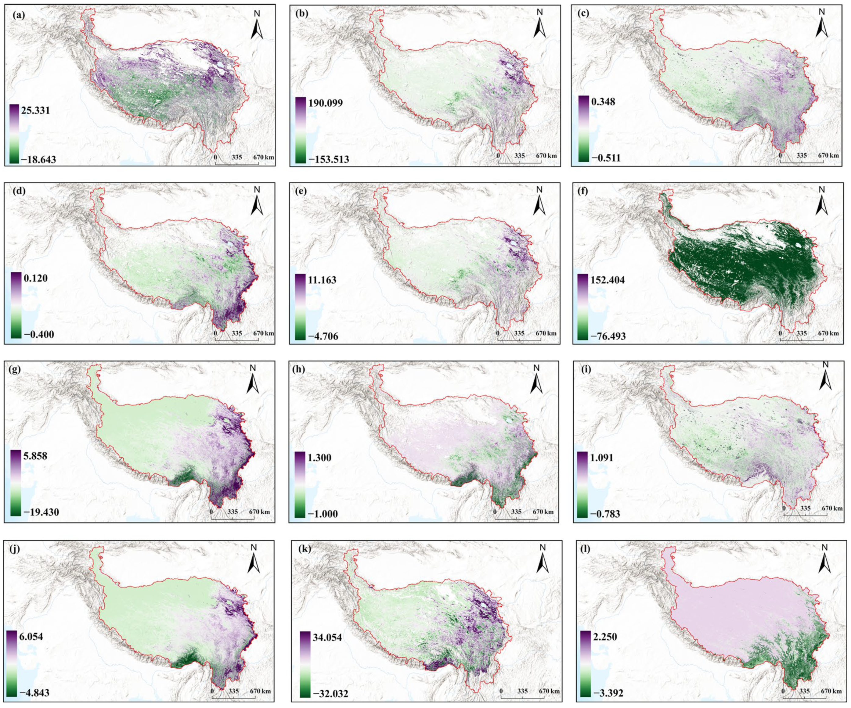
To evaluate the quality and credibility of the embedded research dataset, we analyzed trends using the Mann–Kendall test and Theil–Sen slope estimator. During the previous twenty years, the Tibetan Plateau’s environment has tended to improve, even though some regions have degraded. Signs of photosynthetic activity and vegetation growth in most regions—EVI (Figure 7c), FAPAR (Figure 7d), LAI (Figure 7h), and NDVI (Figure 7i)— showed noticeable upward trends (p < 0.05). The most remarkable advancements occurred in the southern parts of the Qilian Mountains, in the humid southeast, and on the western Sichuan Plateau, where productivity and vegetation coverage drastically increased. Biomass metrics—AGB (Figure 7a), GPP (Figure 7g), NPP (Figure 7j), and TreeCover (Figure 7k)—also demonstrated a comprehensive upward trend but showed significant space-based variability: fast AGB accumulation was apparent in alpine shrublands and southern forest environments of the central–eastern Tibetan Plateau, while some desert–steppe transition zones and alpine meadows exhibited shifts or minor decreases.

The metrics of grassland functions, GYEP (Figure 7b) and RLCCEP (Figure 7e), demonstrated a comprehensive enhancement, with grazing capacity and productivity potential regularly strengthening in the southern and eastern grasslands. However, there is a lingering risk of degradation along the edges. Pressure and disturbance signals (GDGI, Figure 7f) were enhanced in multiple local areas, showing increased pressure resulting from grazing and human activity. This emphasizes the need to consider both sustainable resource use and conservation. Importantly, the EPGP (Figure 7l) demonstrated an overall non-significant or increasing cross-plateau trend, gaining most consistently in the south and east. However, the cold, arid, northwest, and some high-elevation regions had smaller increases in EPGP and exhibited local decreases. This is a general reflection of the space-based distributions of FAPAR, GPP, LAI, NDVI, NPP, and TreeCover, implying that regional ecological products or ecosystem-focused potential for production has strengthened while its vegetation has recovered, whereas its alpine–arid fringes are still vulnerable.

4.1.2. Analysis of Characteristics of Space-Based Differentiation

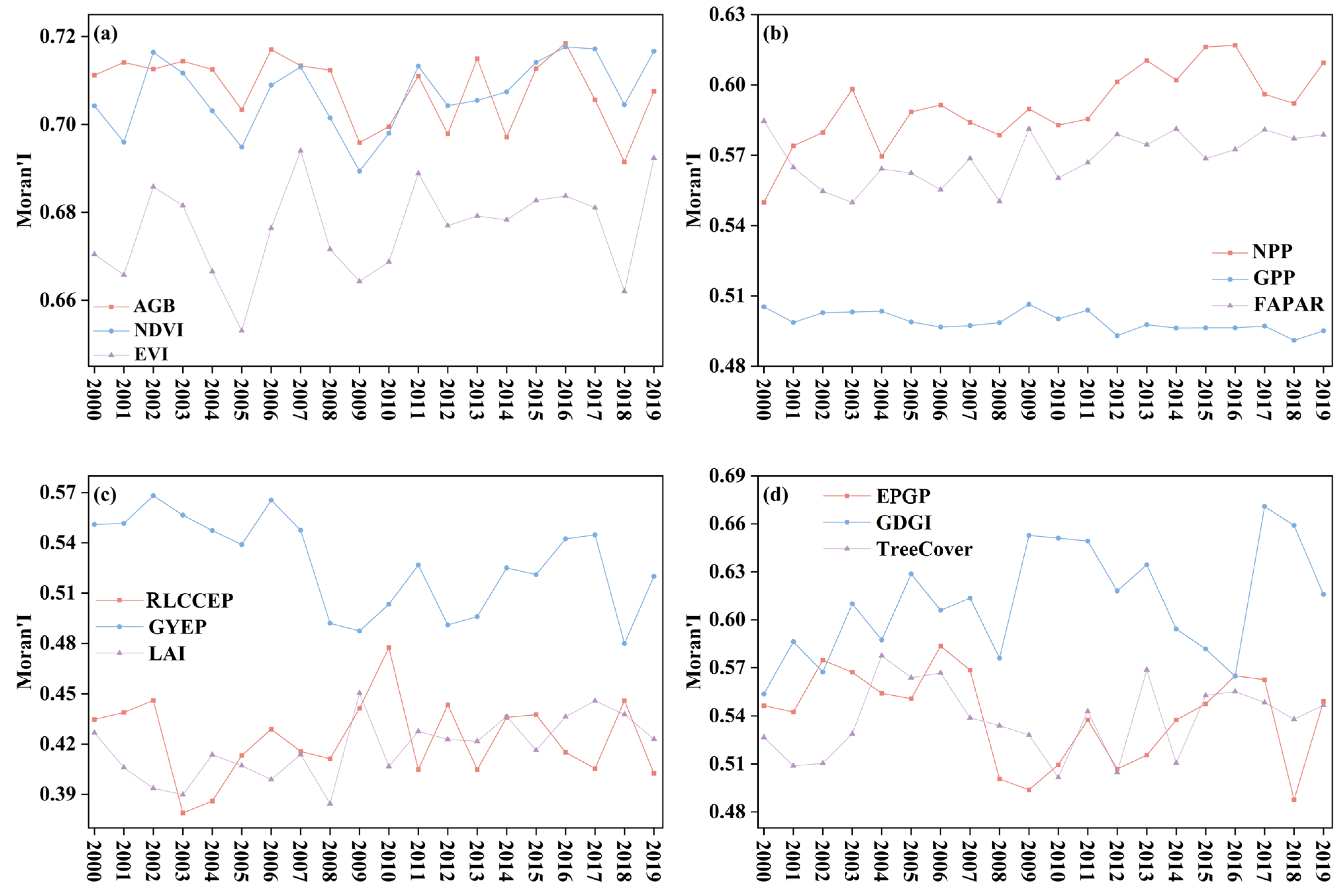
Each variable had Moran’s I values exceeding 0.3, while many of them ranged between 0.5 and 0.8, showing significant positive space-based autocorrelation, highlighting apparent regional consistency and space-based clustering (Figure 8). Productivity and vegetation growth indicators—AGB, EVI, and NDVI (Figure 8a)—frequently had high Moran’s I values, ranging from 0.66 to 0.72. NDVI increased slightly after 2002, with its highest level at 0.72 in 2016, reflecting increased vegetation coverage. AGB regularly exhibited strong agglomeration, often more than 0.70, whereas EVI changed with NDVI. Moran’s I values for photosynthetic efficiency and carbon cycling—NPP, GPP, and FAPAR (Figure 8b)—were somewhat less, between 0.50 and 0.62, but still showed significantly positive autocorrelations. Space-based agglomeration in NPP gradually increased, reaching a maximum of 0.62 in 2015. FAPAR maintained stability at a range between 0.55 and 0.58, while GPP remained near 0.50, indicating that local environmental and climatic shifts have a more pronounced impact on GPP space-based patterns.

The metrics for carrying capacity and grassland ecology (Figure 8c) demonstrated medium levels of agglomeration. GYEP stayed consistent between 0.50 and 0.56, while LAI changed, shifting between 0.38 and 0.45. Initially, the RLCCEP increased and shifted, with a maximum at 0.48 in 2010. Regarding ecological structure and pressure (Figure 8d), TreeCover and GDGI demonstrated Moran’s I values ranging between 0.50 and 0.66, showing moderate to high agglomeration. GDGI had a maximum of 0.67 in 2017, stressing the major space-based concentration of grassland grazing pressure. TreeCover showed an autocorrelation that was somewhat less than that for AGB and NDVI, while gradually retaining its stability. Remarkably, EPGP had less of a space-based autocorrelation while comprehensively increasing (0.40–0.52), as it declined during the early 2010s, but underwent a stable recovery period during the 2010s. This suggests a more understandable space-based trend in the ecological supply of products, matching previous advances in productivity and vegetation factors.

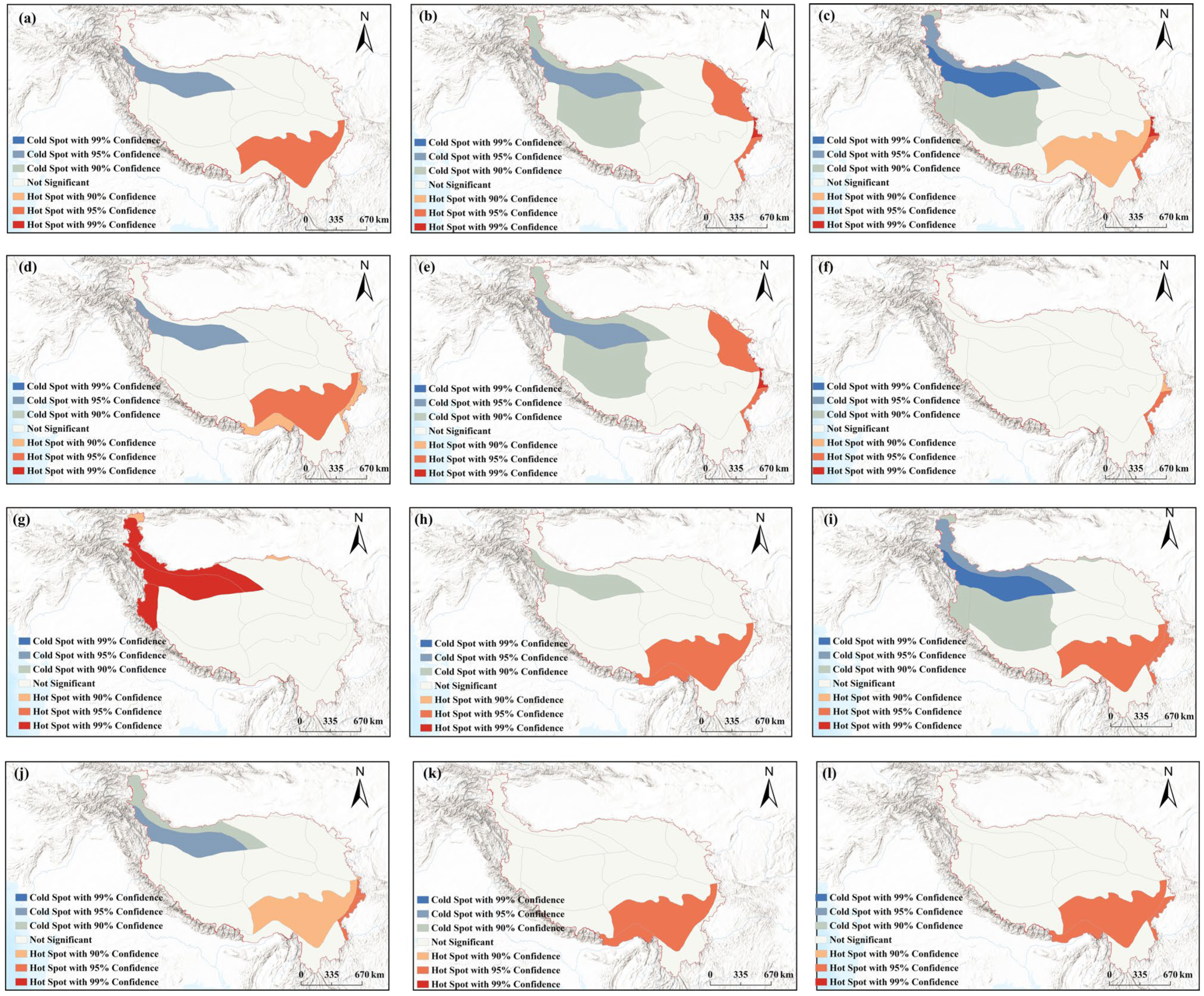
The Tibetan Plateau was divided into cold and hot spots, indicating noticeable regional agglomeration and diverse eco-zonal reactions (Figure 9). Hotspots of above-ground biomass (AGB) (Figure 9a) along with vegetation indexes, such as NDVI (Figure 9i) and EVI (Figure 9c), were mainly in the southern parts of the western Himalayas, eastern Tibetan–western Sichuan alpine gorges, and Yunnan Plateau. These regions are affected by monsoons and are known for their pleasant hydrothermal climate and complicated geography, with high levels of ecosystem productivity, in addition to major potential for sequestration of carbon. In contrast, coldspots were in the Qiangtang Plateau, northern Kunlun Mountains, and Qaidam Basin, demonstrating sparse vegetation, fragile ecosystem functions, and low biomass. Canopy and photosynthetic efficiency variables indicated several similarities: FAPAR (Figure 9d) showed a constant belt of hotspots throughout the gorge–valley and humid southeast systems, whereas LAI (Figure 9h) had a closely related but somewhat narrower band. Coldspots for each variable were mainly located in the high-elevation interior regions and Qaidam-Tarim dry belt, stressing hydrothermal-related restrictions on radiation absorption and canopy development. Metrics of carbon cycle production, such as NPP (Figure 9j) and GPP (Figure 9g), are usually linked to hotspots of vegetation indices, with maximum values in the humid southeast regions and cold areas in high-elevation and arid interior locations, demonstrating a robust space-based link connecting carbon uptake with vegetation activity.

Carrying capacity and grassland ecology have unique patterns: GYEP hotspots (Figure 9b) extend from humid southeast areas into eastern Qilian-Qinghai and the wide valleys of southern Qinghai. In contrast, RLCCEP hotspots (Figure 9e) were mainly in valley terraces and southeastern plateaus. Coldspots for both these factors were located on the freezing interior and Kunlun mountain plateaus, emphasizing the importance of natural limitations. Structural indicators and ecological pressure, EPGP (Figure 9l), TreeCover (Figure 9k), and GDGI (Figure 9f), also demonstrated heterogeneous space. Southeastern and southern Tibet contain GDGI hotspots, suggesting increased pressure on grazing areas. TreeCover hotspots were related to the forest–eastern mountain belt, whereas coldspots appeared in alpine grassland and desert regions, showing the integrated influence of topography and climate. The EPGP tended to mirror the GDGI, an indication of varied space during pastoral activities and the intensity of land use throughout plateau ecosystems.

4.1.3. Field Data Validation

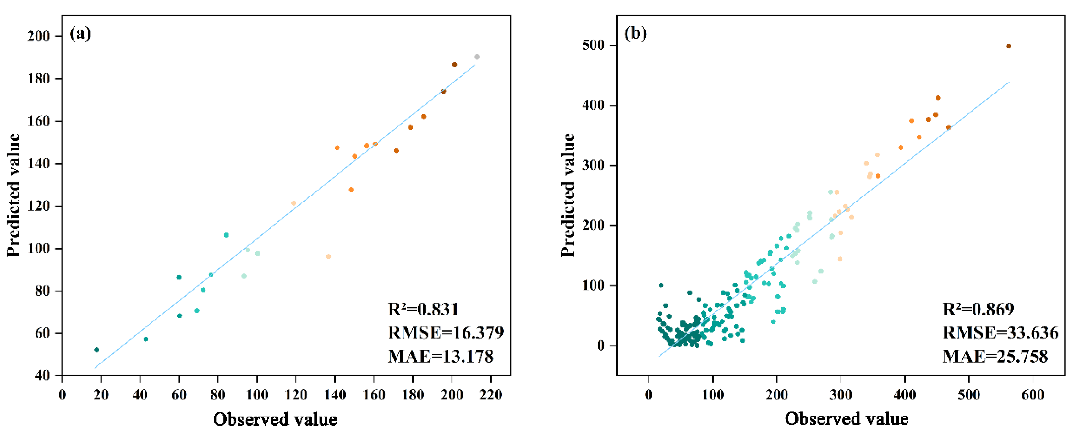
This research evaluated the ecological and reliability fidelity of a set of ESE data based on field validation data. It considered AGB measurements from 2005 and 2019 and a set of 2000 vegetation survey data to further verify vegetation conditions. This shows that the estimates from the field observations and ESE were strongly correlated (Figure 10). In 2005, the validation results indicated that R² = 0.8310, RMSE = 16.38, and MAE = 13.18 (Figure 10a). In contrast, the 2019 validation yielded R² = 0.8690, RMSE = 33.64, and MAE = 25.76 (Figure 10b). These results demonstrate minimal predictive bias and high-fit accuracy for each of these periods of time.

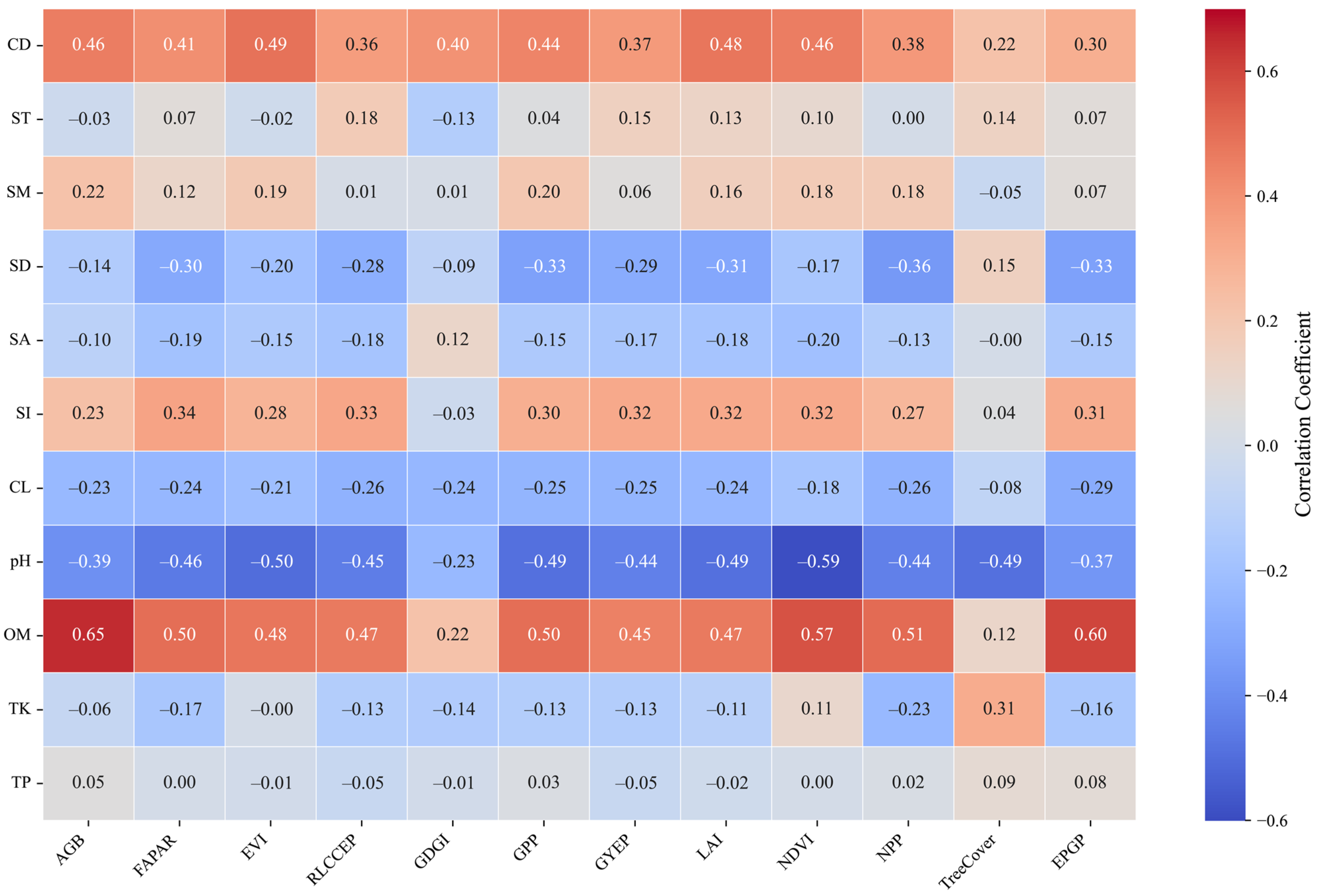
Another approach to validation requires analyzing correlations connecting the ecological characteristics within this set and field-based observations to evaluate the accuracy of representation. The findings showed that most ecological variables and embeddings were significantly correlated, suggesting that embedded aspects accurately depicted the ecosystem’s environmental gradients and space-based diversity (Figure 11). Organic matter was the individual indicator that was most strongly correlated with the ESE data, indicating the presence of significantly positive relationships with AGB (r = 0.65), NDVI (r = 0.57), and FAPAR (r = 0.50). This suggests that parameters for canopy photosynthetically active radiation absorption, in addition to vegetation productivity, are an effective reflection of space-based differences in the nutrient content of the soil. Moreover, grassland coverage had medium to strongly positive correlations (0.36–0.49) with ecological indicators, confirming how these embeddings effectively captured patterns of vegetation coverage. In contrast, soil pH was negatively correlated (−0.37 to −0.59) with ecological indicators, highlighting potential regulatory limitations that soil pH imposes on ecosystem organization and vegetation growth.

4.2. Prediction Analysis Based on the Prithvi-EO Model

4.2.1. Prediction Results

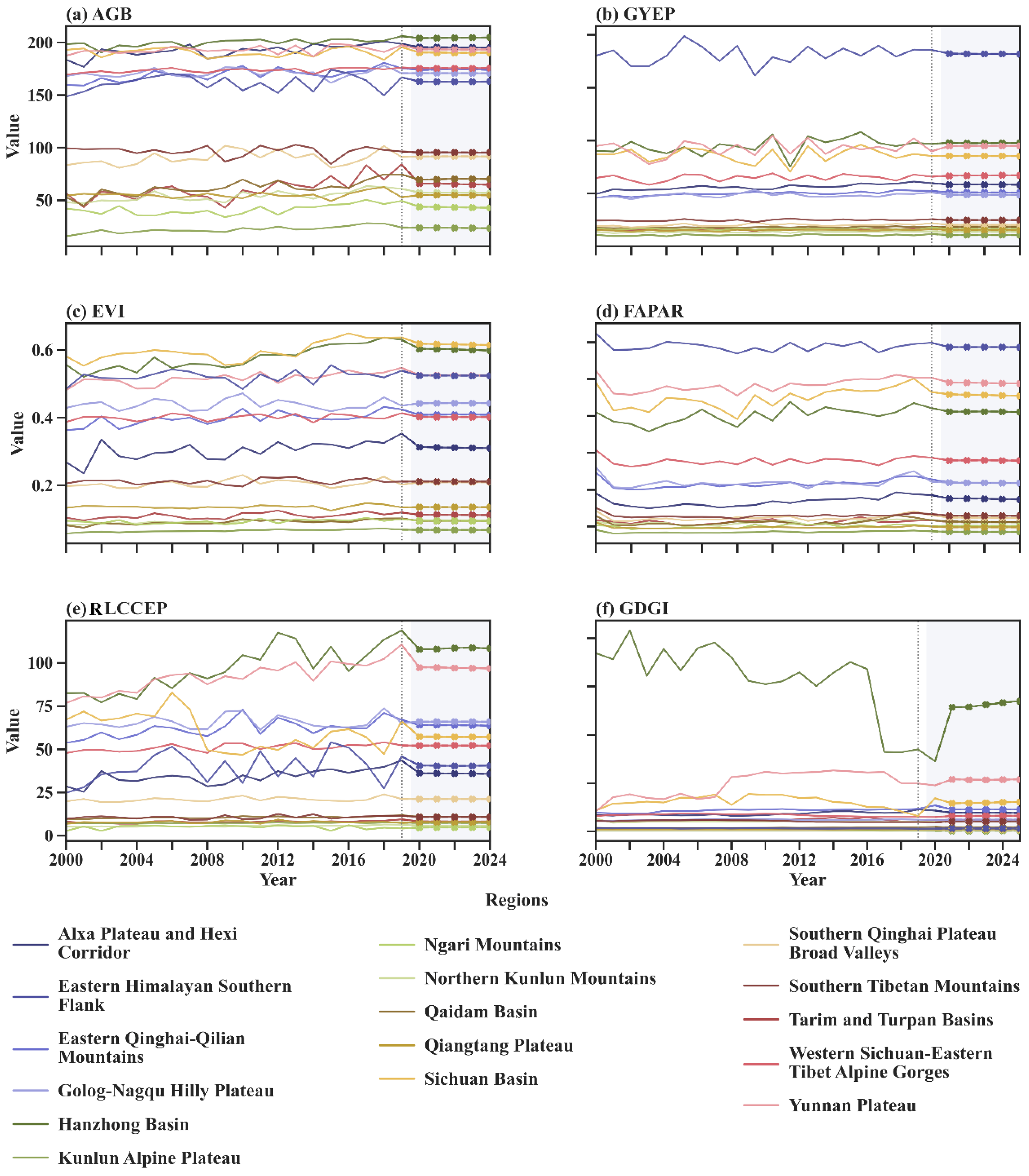
The Prithvi-EO model was implemented to predict the temporal evolution of important ecological indicators in the Tibetan Plateau. The results were evaluated, along with ecological and geographical division statistics, to highlight the long-term interactions of ecological aspects. Figure 12 shows the trends of the unique function-based gradients, comprehensive improvements, and major regional differences. Throughout the previous twenty years, the majority of indicators have displayed continued enrichment or retained heightened values. AGB, an important vegetation productivity indicator (Figure 12a), revealed limited instances of stability or growth within several regions, especially with ideal heat and water scenarios, including the wide valleys of the southern Tibetan Plateau, southeastern Himalayas, eastern Tibetan Plateau, and Golog-Nagqu Hilly Plateau. These regions have retained high levels of AGB and should increase slightly after 2020, hinting at a reliably structured ecosystem along with a robust recovery of vegetation. In contrast, arid areas, such as the Hexi Corridor, Turpan and Tarim Basins, Hexi Corridor, Qaidam Basin, and Alashan, produced remarkably reduced values for AGB. Despite this, the comprehensive trend showed slow growth, implying a careful process of recovery within dry ecosystems due to human intervention, as well as natural regeneration. The growth of vegetation metrics like FAPAR and EVI reflected the general trends noticed in AGB but displayed more apparent region-based differences (Figure 12c,d). The southern gorges and eastern mountain areas (such as the Sichuan Basin, eastern Sichuan Plateau, and southeastern Himalayas) gradually sustained high FAPAR and EVI values, showing a major potential for photosynthesis and extensive vegetation growth. In contrast, areas like the Qaidam Basin, Hexi Corridor, and Alashan had lower values, indicating the extended prevention of vegetation growth resulting from climate-related limitations and limits on water.

GYEP, an essential way of measuring the productivity of grassland ecosystems, showed noticeable variations between regions (Figure 12b). Since 2010, regions containing densely distributed grassland, such as the Kunlun Mountains, Qiangtang Plateau, and southern Tibetan Plateau, have preserved high GYEP with limited shifts, showing that the ecosystem’s ability to produce is gradually stabilizing. However, areas such as the Hexi Corridor and arid basins showed less and more irregular productivity, stressing increases in ecological vulnerability and climatic sensitivity. RLCCEP, the pastoral indicator of carrying capacity, also showed noticeable differences across regions (Figure 12e). Crucial regions of grassland, such as the southern Tibetan Plateau, Kunlun Mountain Plateau, and Qiangtang Plateau, have undergone large increases in RLCCEP since 2000, indicating constantly enhanced grazing potential and ecological capacity. In contrast, the eastern agricultural-pastoral zone of transition, as well as desert regions, typically had limits in growth. The GDGI (Figure 12f) started by fluctuating but eventually grew within many areas, especially within pastoral regions such as the Golog-Nagqu Hilly Plateau and the Kunlun Mountain Plateau. It is worth noting that after 2015, the GDGI increased again, implying a transition to increasingly sustainable pressure on grazing, matching the accelerating trend towards greater carrying capacity.

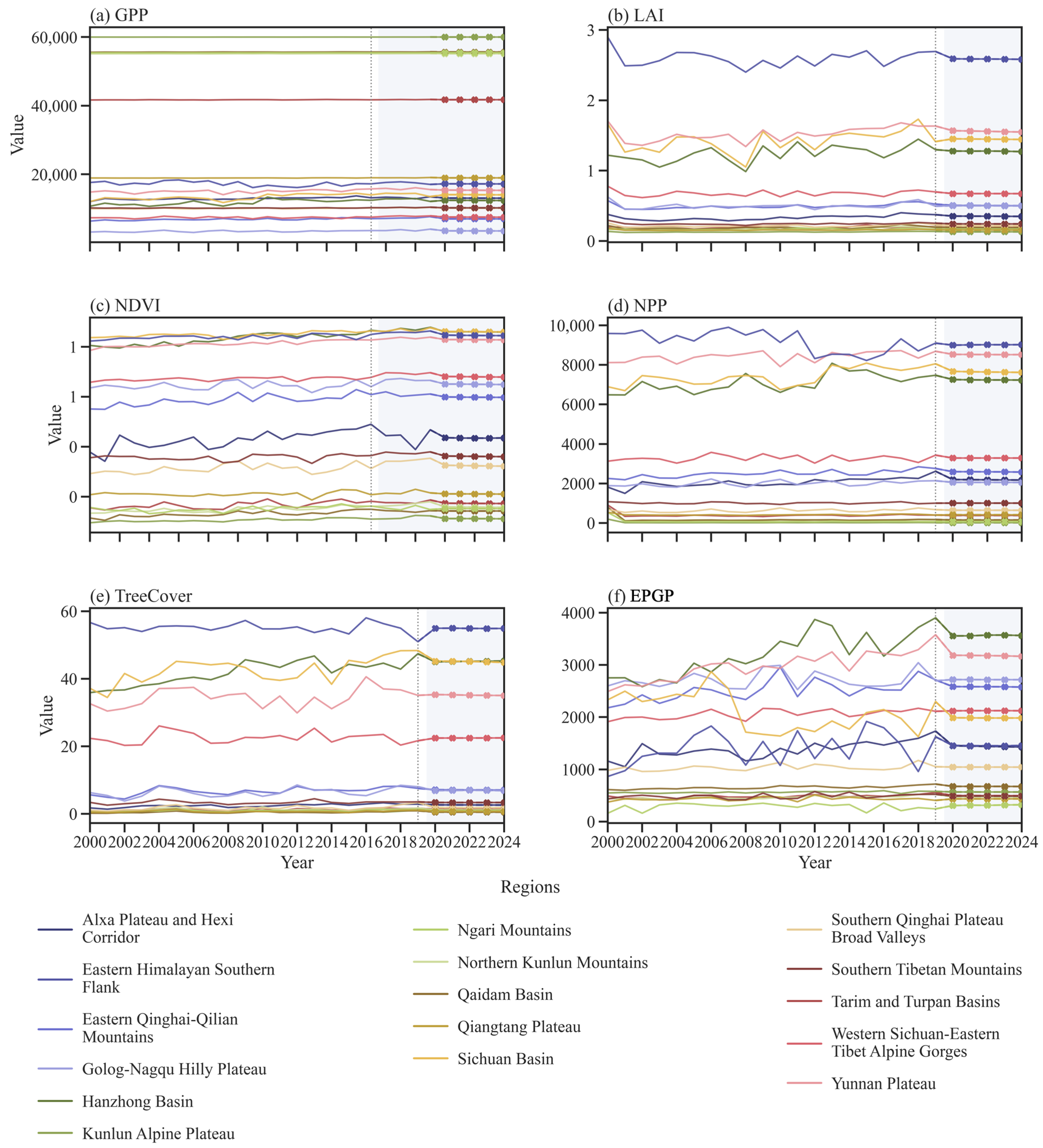
Figure 13 stresses major region-based trends and disparities, depicting the space and temporal complex nature of ecosystem function and structure in the Tibetan Plateau’s difficult climate and terrain. The general GPP trend was stable and regular (Figure 13a). Areas such as the Southern Kunlun Mountains and Kunlun Plateau constantly demonstrated high extents with limited growth throughout forecasting, illustrating strong productivity of vegetation and a capacity for ecological progress. In contrast, cold or dry areas, including the Qaidam Basin, Qiangtang Plateau, along with the Hexi Corridor and Altyn-Tagh Mountains, showed lower and more stable GPP values, implying major limitations on productivity as a result of water and climate restrictions. Trends of NPP reflected those of GPP (Figure 13d), as high values were mainly in areas containing advantageous heat and water scenarios, such as the southern Yunnan Plateau, valleys of the southern Tibetan Plateau, and southern parts of the eastern Himalayas, demonstrating strong examples of main productivity and potential for fixation of carbon. However, dry areas, including the Hexi Corridor and Altyn-Tagh Mountain, as well as the Qaidam Basin, had lower levels of NPP, but lacked definite trends. LAI showed specific variations between regions (Figure 13b). Monsoon-influenced areas, like the southern Yunnan Plateau and the southern parts of the eastern Himalayas, retained higher and gradually rising values of LAI, mirroring constant improvements in the structure of vegetation communities. In contrast, dry areas, such as the Hexi Corridor and Altyn-Tagh Mountains, as well as the Qaidam Basin, had reduced and less frequently shifting LAI values, showing an ecosystem with a less complicated structure.

The temporal changes in the NDVI indicated a stable rise in vegetation coverage (Figure 13c), particularly following 2020 in areas such as the valleys of the southern Tibetan Plateau and the southern Yunnan Plateau, demonstrating improved vegetation growth despite a warming climate. In contrast, the Qaidam Basin and Qiangtang Plateau had consistently limited gradually shifting values for NDVI, implying limited vegetation coverage. Space-based differences in TreeCover were noticeable (Figure 13e), as there were increased levels in the southern Yunnan Plateau and eastern Qilian-Qinghai Mountains, showing a limited, gradual rise. Moreover, the Qaidam Basin and Qiangtang Plateau retained stable and limited levels of TreeCover without major shifts in vegetation patterns. The time series for the EPGP describes the space-based arrangement of functions for ecosystem potential, while areas with high values are mostly in the southern parts of the eastern Himalayas, valleys of the southern Tibetan Plateau, and southern Yunnan Plateau, showing a slow increase (Figure 13f). In contrast, the areas with low values in the Hexi Corridor and Altyn-Tagh Mountains, in addition to the Qaidam Basin, imply a limited amount of ecological potential and an increased level of ecosystem-focused weakness.

4.2.2. Validation of Model Prediction Accuracy

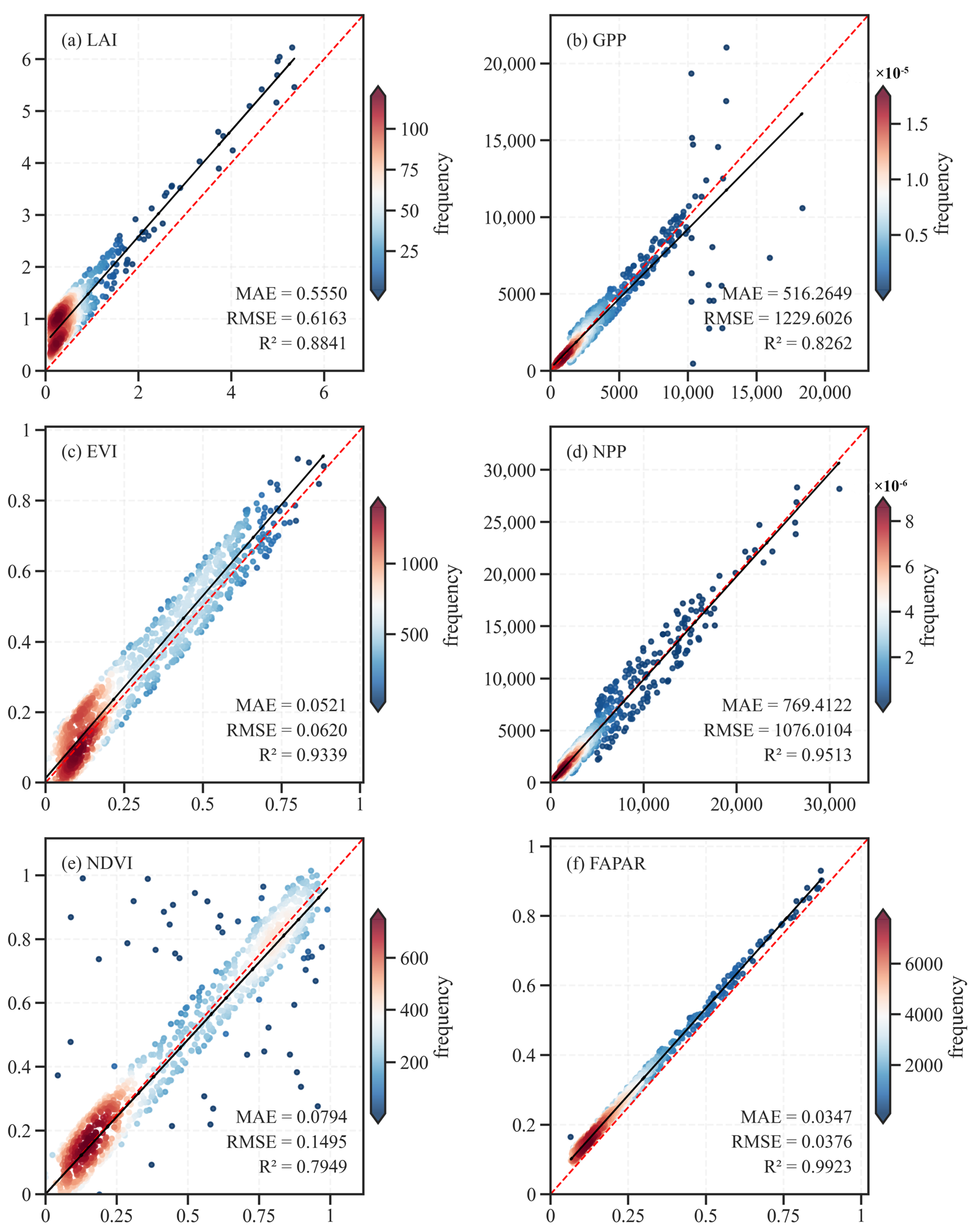
This research assessed the precision and reliability of predictions regarding ecological indicators with the Prithvi-EO model based on data from 2000 to 2024 according to two benchmarks: a combination of field observations and remote sensing inversion data. Quantitative evaluations of six ecological variables, LAI, GPP, EVI, NPP, NDVI, and FAPAR, were implemented to confirm data accuracy (Figure 14). This model demonstrated robustness and remarkable performance in the predictions of the indicators. It is worth noting that FAPAR had the highest correlation (Figure 14f), with an R² of 0.9923 and RMSE and MAE values of 0.04 and 0.03. This highlights the sustained capacity of the model to recreate fractions of light absorbed by plants and precisely mirror each region’s ecosystem function and photosynthetic efficiency. The levels of predictive accuracy for NPP and EVI were also outstanding (Figure 14c,d), with R² values of 0.9513 and 0.9339 and RMSE values of 1076.01 and 0.06, emphasizing the model’s ability to embody changes in the vitality and carbon fixation of vegetation.

The predicted values for GPP and LAI demonstrated acceptable accuracy levels (Figure 14a,b). Its R² values were 0.8262 and 0.8841, respectively, indicating that the model can proficiently replicate changes in the region’s structure of leaf area, as well as the temporal aspects of main productivity. Although the MAE (516.26) and RMSE (1229.60) for GPP were comparatively high, the overall trend matched the data, and its differences were primarily the result of unusual shifts within certain areas. NDVI’s prediction accuracy was somewhat less (Figure 14e), with an R² of 0.7949; despite this, it stayed inside a reasonable amount. This confirms that the model is highly capable of capturing holistic space and temporal vegetation coverage patterns.

4.3. Comprehensive Reasoning Representation Results Based on GeoChat

Table 2. Long-term mean and interannual variability of AGB, GYEP, and EVI across 18 geographical subregions of the Tibetan Plateau.

Name	AGB		GYEP		EVI
	μ	sd	μ	sd	μ	sd
Tarim and Turpan Basins	1.90	1.72	1.70	1.84	1.42	−1.48
Alxa Plateau and Hexi Corridor	0.73	0.59	0.56	0.60	0.45	−0.47
Northern Kunlun Mountains	3.29	3.07	3.05	3.28	2.54	−2.64
Kunlun Alpine Plateau	5.35	5.07	5.07	5.44	4.24	−4.40
Qaidam Basin	10.15	9.66	9.68	10.36	8.05	−8.28
Central Shanxi-Northern Shaanxi-Eastern Gansu Plateau and Hills	0.73	0.59	0.56	0.60	0.45	−0.47
Eastern Qinghai-Qilian Mountains	7.90	7.51	7.53	8.09	6.28	−6.51
Southern Shanxi-Guanzhong Basin	0.73	0.59	0.56	0.60	0.45	−0.47
Ngari Mountains	7.04	6.72	6.74	7.21	5.64	−5.85
Southern Qinghai Plateau Broad Valleys	34.46	32.95	33.08	35.21	27.38	−27.92
Qiangtang Plateau	18.37	17.59	17.66	18.81	14.67	−15.03
Golog-Nagqu Hilly Plateau	45.18	43.04	43.20	45.80	35.58	−36.00
Hanzhong Basin	0.73	0.59	0.56	0.60	0.45	−0.47
Western Sichuan-Eastern Tibet Alpine Gorges	17.99	17.07	17.11	18.15	14.09	−14.26
Sichuan Basin	0.73	0.59	0.56	0.60	0.45	−0.47
Yunnan Plateau	0.74	0.59	0.56	0.61	0.46	−0.47
Eastern Himalayan Southern Flank	13.89	13.16	13.19	13.98	10.86	−10.99
Southern Tibetan Mountains	11.82	11.23	11.26	11.96	9.32	−9.49

Note: μ denotes the long-term mean and sd interannual variability. Negative values result from standardization and indicate relative levels, while |sd| reflects variability. Standardization does not affect the interpretation of regional disparities or rankings. All variables are dimensionless and comparable across variables. The same applies below.

describes the basic patterns and fluctuation aspects of GYEP, EVI, and AGB, emphasizing their yearly changes and future methods from 2000 to 2024. The results indicated a regularly present zone section in the space-based arrangement of these variables. This section stretches from dry to semi-dry basins, such as the Turpan and Tarim Basins, Hexi Corridor, and Alxa Plateau, amidst gorge zones and mountain edges, ending in high-cover and high-altitude core regions, including the Golog-Nagqu Hilly Plateau and the Southern Qinghai Plateau Broad Valleys, Qiangtang Plateau. Within these areas, the long-term mean monotonically increased. At the same time, yearly changes also increased, leading to ‘low level–low variability’ along with ‘high level–high variability’. Unusually high-value areas, like the Qiangtang Plateau, Golog-Nagqu Hilly Plateau, and Southern Qinghai Plateau Broad Valleys indicated drastically higher values for each indicator in comparison with other areas. However, low mountain terraces and basins tend to have limited differences and reduced values.

An inter-indicator comparison showed a general alignment between structure and activity over several years. The long-term mean values of AGB, GYEP, and EVI were highly consistent, indicating a strong connection between biomass/aboveground productivity and greenness. However, the EVI displayed more pronounced interannual variability in the medium-high and extremely high value regions. This suggests that visible and near-infrared greenness is more sensitive to annual climatic conditions, snow–freeze cycles, and the length of the growing season. In contrast, AGB’s interannual variability of AGB was relatively moderate, reflecting the inertia of biomass over time.

Table 3. Long-term mean and interannual variability of FAPAR, RLCCEP, and GDGI across 18 geographical subregions of the Tibetan Plateau.

Name	FAPAR		RLCCEP		GDGI
	μ	sd	μ	sd	μ	sd
Tarim and Turpan Basins	1.54	−1.53	1.43	1.02	−1.56	1.68
Alxa Plateau and Hexi Corridor	0.50	−0.49	0.53	0.17	−0.52	0.60
Northern Kunlun Mountains	2.76	−2.73	2.50	1.95	−2.75	2.94
Kunlun Alpine Plateau	4.59	−4.54	4.08	3.41	−4.56	4.83
Qaidam Basin	8.76	−8.58	7.73	6.51	−8.60	9.13
Central Shanxi-Northern Shaanxi-Eastern Gansu Plateau and Hills	0.50	−0.49	0.53	0.17	−0.52	0.60
Eastern Qinghai-Qilian Mountains	6.83	−6.71	6.02	5.11	−6.74	7.14
Southern Shanxi-Guanzhong Basin	0.50	−0.49	0.53	0.17	−0.52	0.60
Ngari Mountains	6.08	−6.04	5.39	4.61	−6.06	6.39
Southern Qinghai Plateau Broad Valleys	29.85	−29.04	26.22	22.20	−29.03	30.86
Qiangtang Plateau	15.93	−15.61	14.01	11.96	−15.60	16.53
Golog-Nagqu Hilly Plateau	38.92	−37.60	34.27	28.38	−37.57	40.15
Hanzhong Basin	0.50	−0.49	0.53	0.17	−0.52	0.60
Western Sichuan-Eastern Tibet Alpine Gorges	15.42	−14.90	13.63	11.12	−14.90	15.95
Sichuan Basin	0.50	−0.49	0.53	0.17	−0.52	0.61
Yunnan Plateau	0.51	−0.49	0.54	0.17	−0.52	0.61
Eastern Himalayan Southern Flank	11.88	−11.48	10.52	8.52	−11.49	12.31
Southern Tibetan Mountains	10.14	−9.88	8.98	7.41	−9.89	10.55

presents the long-term means and interannual variabilities of FAPAR, RLCCEP, and GDGI from 2000 to 2024. The long-term mean values of FAPAR and RLCCEP follow a productivity gradient: they are low in arid to semi-arid basins (e.g., Tarim and Turpan Basins, Alxa Plateau, and Hexi Corridor), increase at mountain edges and gorge transition zones, and peak in cold, high-cover core regions (e.g., Southern Qinghai Plateau Broad Valleys, Golog–Nagqu Hilly Plateau, and Qiangtang Plateau). Correspondingly, interannual variability increases, creating patterns of “low level–low variability” and “high level–high variability.” Regions with exceptionally high values, such as the Golog–Nagqu Hilly Plateau (long-term mean FAPAR = 38.92, long-term mean RLCCEP = 34.27, |interannual variability| FAPAR = 37.60, and interannual variability | RLCCEP = 28.38) and Southern Qinghai Plateau Broad Valleys (long-term mean FAPAR = 29.85, long-term mean RLCCEP = 26.22, |interannual variability| FAPAR = 29.04, and |interannual variability| RLCCEP = 22.20), significantly surpassed the others. In contrast, arid basins and terraces generally exhibited low values.

A comparison of the indicators revealed a close alignment between the long-term mean values of FAPAR and RLCCEP, indicating synchronous fluctuations in the canopy-absorbed photosynthetically active radiation and ecosystem status over multiple years. Interannual variability was notably amplified in cold, high-cover regions, suggesting heightened sensitivity to year-to-year water-thermal variations and snow-freeze cycles. In contrast, the long-term mean GDGI remained consistently negative across the region, with a larger negative amplitude in areas characterized by “high cover—high productivity” (e.g., long-term mean Golog-Nagqu Hilly Plateau GDGI = −37.57; long-term mean Southern Qinghai Plateau Broad Valleys GDGI = −29.03), maintaining an inverse gradient with FAPAR and RLCCEP. The interannual variability in GDGI is also amplified in these high-value regions (i.e., 40.15 and 30.86, respectively), indicating a pronounced response to year-to-year climate fluctuations along the dry-wet gradient or drought intensity.

The annual changes and long-term average values of LAI, NDVI, and GPP from 2000 to 2024 are shown in

Table 4. Long-term mean and interannual variability of GPP, LAI, and NDVI across 18 geographical subregions of the Tibetan Plateau.

Name	GPP		LAI		NDVI
	μ	sd	μ	sd	μ	sd
Tarim and Turpan Basins	1.39	−1.69	−1.30	−1.52	1.12	1.50
Alxa Plateau and Hexi Corridor	0.43	−0.53	−0.40	−0.48	0.25	0.48
Northern Kunlun Mountains	2.47	−3.02	−2.36	−2.72	2.08	2.69
Kunlun Alpine Plateau	4.13	−5.05	−3.94	−4.52	3.57	4.49
Qaidam Basin	7.75	−9.57	−7.57	−8.57	6.73	8.54
Central Shanxi-Northern Shaanxi-Eastern Gansu Plateau and Hills	0.43	−0.53	−0.40	−0.48	0.25	0.48
Eastern Qinghai-Qilian Mountains	6.11	−7.50	−5.87	−6.72	5.31	6.68
Southern Shanxi-Guanzhong Basin	0.43	−0.53	−0.40	−0.49	0.25	0.48
Ngari Mountains	5.50	−6.71	−5.24	−6.01	4.80	5.96
Southern Qinghai Plateau Broad Valleys	26.03	−32.42	−25.94	−28.99	22.73	29.02
Qiangtang Plateau	14.05	−17.38	−13.81	−15.55	12.30	15.52
Golog-Nagqu Hilly Plateau	33.40	−42.00	−33.91	−37.52	28.99	37.70
Hanzhong Basin	0.43	−0.53	−0.40	−0.49	0.25	0.48
Western Sichuan-Eastern Tibet Alpine Gorges	13.22	−16.63	−13.41	−14.86	11.40	14.93
Sichuan Basin	0.43	−0.53	−0.40	−0.49	0.25	0.48
Yunnan Plateau	0.43	−0.54	−0.41	−0.49	0.26	0.48
Eastern Himalayan Southern Flank	10.19	−12.81	−10.32	−11.45	8.76	11.49
Southern Tibetan Mountains	8.83	−11.01	−8.80	−9.84	7.64	9.85

. The space-based arrangement of these average values matches the topographic and hydrothermal sections. Reduced average values were identified in dry to semi-dry areas, such as the Turpan and Tarim Basins, Hexi Corridor, and Alxa Plateau. These become higher along gorge regions and mountain edges, attaining higher elevations in cold, core areas with dense vegetation, including the Golog-Nagqu Hilly Plateau, Southern Qinghai Plateau Broad Valleys, and Qiangtang Plateau. In these regions, yearly changes also increase, creating patterns such as ‘low level—low changes and ‘high level–high changes’. Remarkably, the Golog-Nagqu Hilly Plateau indicated high values, involving an NDVI of 28.99, a long-term mean GPP of 33.40, and yearly changes of 37.70 for NDVI and 42.00 for GPP. The Southern Qinghai Broad Valleys are also noteworthy, including an NDVI of 22.73, a long-term mean GPP of 26.03, and yearly changes of 29.02 for NDVI and 32.42 for GPP. In contrast, terraces and basins, such as the Sichuan Basin, Hexi Corridor, and Alxa Plateau, typically had the lowest values.

Multiple indicators were compared, revealing robust stability and hierarchy-based differences, while long-term mean NDVI and GPP values were closely aligned, indicating that function and structure changed simultaneously over several years. The long-term mean LAI values had a regional-based ranking that resembled GPP and NDVI. Despite this, its yearly changes drastically intensified in cold and densely vegetated areas, such as the Qiangtang Plateau, Southern Qinghai Plateau Broad Valleys, and Golog-Nagqu Hilly Plateau. This indicates that the structure of canopies responds more readily to shifts in each year’s length of growing season, patterns of snowmelts and freezing, and atypical hydrothermal occurrences. In contrast, the variability and values of each indicator remain low in terraces and basins, mirroring a stable habit described as ‘limited-water—low activity—low changes.

Table 5. Long-term mean and interannual variability of NPP, TreeCover, and EPGP across 18 geographical subregions of the Tibetan Plateau.

Name	NPP		TreeCover		EPGP
	μ	sd	μ	sd	μ	sd
Tarim and Turpan Basins	−1.75	−1.12	−1.83	−1.44	−1.44	0.84
Alxa Plateau and Hexi Corridor	−0.58	−0.25	−0.64	−0.46	−0.43	0.10
Northern Kunlun Mountains	−3.13	−2.08	−3.22	−2.57	−2.64	1.62
Kunlun Alpine Plateau	−5.18	−3.57	−5.31	−4.27	−4.42	2.87
Qaidam Basin	−9.87	−6.72	−10.05	−8.12	−8.49	5.39
Central Shanxi–Northern Shaanxi–Eastern Gansu Plateau and Hills	−0.58	−0.25	−0.64	−0.46	−0.43	0.10
Eastern Qinghai-Qilian Mountains	−7.71	−5.30	−7.85	−6.35	−6.61	4.29
Southern Shanxi-Guanzhong Basin	−0.58	−0.26	−0.64	−0.46	−0.43	0.10
Ngari Mountains	−6.87	−4.79	−7.03	−5.66	−5.90	3.89
Southern Qinghai Plateau Broad Valleys	−33.58	−22.65	−34.03	−27.59	−29.08	18.06
Qiangtang Plateau	−17.94	−12.25	−18.23	−14.75	−15.51	9.85
Golog-Nagqu Hilly Plateau	−43.73	−28.88	−44.27	−35.85	−37.91	22.60
Hanzhong Basin	−0.58	−0.26	−0.64	−0.46	−0.43	0.10
Western Sichuan-Eastern Tibet Alpine Gorges	−17.33	−11.36	−17.58	−14.20	−14.98	8.83
Sichuan Basin	−0.58	−0.26	−0.64	−0.46	−0.43	0.10
Yunnan Plateau	−0.60	−0.26	−0.64	−0.47	−0.43	0.10
Eastern Himalayan Southern Flank	−13.35	−8.73	−13.56	−10.93	−11.52	6.76
Southern Tibetan Mountains	−11.42	−7.61	−11.62	−9.37	−9.85	5.98

illustrates the yearly changes and long-term means of EPGP, TreeCover, and NPP between 2000 and 2024. In terms of space, the long-term mean TreeCover and NPP rankings were consistent. Low-mountain terraces and dry to semi-dry basins, such as the Alxa Plateau, Hexi Corridor, and Tarim and Turpan Basins. Their values rise through the gorge and mountain edge zones, attaining greater heights in high-cover, cold-core areas, including the Southern Qinghai Plateau Broad Valleys, Qiangtang Plateau, and Golog-Nagqu Hilly Plateau, with gradually increasing negative values. This is shown in yearly changes, creating paired ‘low level–low changes’ and ‘high level–high changes.’ EPGP resembles this trend, having negative levels for the long-term mean and its yearly changes rising in high-cover, cold areas. This implies an integrated attitude of a topography-related context with ecological structures and functions, in addition to enhanced responses to these changes.

A regional comparison showed that areas with extremely high values and variability were concentrated in cold, high-cover regions, such as the Golog-Nagqu Hilly Plateau (long-term mean NPP = −43.73, long-term mean TreeCover = −44.27, |interannual variability| NPP = 28.88, |interannual variability| TreeCover = 35.85) and the Southern Qinghai Plateau Broad Valleys (long-term mean NPP = −33.58, long-term mean TreeCover = −34.03, |interannual variability| NPP = 22.65, |interannual variability| TreeCover = 27.59), significantly surpassing other regions. These are followed by the Qiangtang Plateau and the Western Sichuan-Eastern Tibet Alpine Gorges. The medium–high value and medium–high variability group, including areas such as the Eastern Qinghai-Qilian Mountains, Ngari Mountains, Eastern Himalayan Southern Flank, and Southern Tibetan Mountains, showed simultaneous increases in both indicators and |interannual variability|, highlighting the sensitivity of topographic-climatic transition zones. Meanwhile, the low-value and low-variability groups, such as the Tarim and Turpan Basins, Alxa Plateau and Hexi Corridor, Central Shanxi-Northern Shaanxi-Eastern Gansu Plateau and Hills, Sichuan Basin, and Yunnan Plateau, exhibited relatively lower NPP and coverage levels with minor interannual fluctuations, indicating a water-limited equilibrium.

5. Discussion

This research proposes a two-stage structure—unified embedding and comprehensive reasoning—to carefully describe the Tibetan Plateau’s ecological function and structure from 2000 to 2024. By combining LLMs with satellite embedding approaches, we developed a cohesive space and temporal representative structure that tackles long-term problems regarding interpretability, temporal stability, and fusion of data with multiple sources. The Mann–Kendall trend analyses and the Theil-Sen slope, along with Moran’s I space-based autocorrelation statistics, demonstrate extensive ecological enhancements with major space-based agglomeration (Moran’s I value of 0.50–0.80). Prithvi-EO time-series predictions indicated significant correlations with field observations (NPP R² = 0.9513; FAPAR R² = 0.9923), while GeoChat-CRF created comprehensible dimensions connecting space-based organization, stability, structure, and function. These findings enrich the ecological awareness and methodology-linked capacities of the Tibetan Plateau’s complex mechanisms.

5.1. Methodological Advances and Data Product Significance

The ESE research model combines semantics by embedding 12 different ecological variables, including AGB, GPP, LAI, NDVI, and NPP, into a reasonable structure based on space and time. In contrast with typical integrated indexes that sequentially add surface parameters together [10], this model implements self-supervised contrastive learning to find distribution-based patterns lacking certain constraints on tasks, developing constant fields of vectors with coherent space. This helps to solve the lack of consistency due to temporal gaps, sensor variations, and fluctuating resolutions within the original data. Positive trends (p < 0.05) noticed in the majority of variables between 2000 and 2019, as well as high Moran’s I values, suggest that ESE retains large-scale zone sections while guaranteeing consistency in various regions, which is considered a crucial aspect of future ecosystem monitoring [18].

Temporal completion with Prithvi-EO increased the embedding sequence to 2020–2024, turning a historical record into an almost-real-time monitoring method. This model produced highly accurate predictions (RMSE = 0.04, FAPAR R² = 0.9923; RMSE = 1076.01, NPP R² = 0.9513), confirming its capacity to guess yearly interactions in high-altitude areas with limited on-site observations [28]. This exceeds past remote-sensing evaluations that were solely based on optical imagery, which were limited by coarse temporal resolution and cloud interference. Prithvi-EO’s incorporation of temporal self-attention approaches and priors with multiple sources enables it to portray long-term tendencies, season-based cycles, and relationships related to combinations of multiple variables more effectively than existing ways of filling gaps.

The GeoChat-CRF structure signals a transition from unclear embedding forms to easily understandable descriptions of ecological concepts. It does not rely on obscure latent elements, but arranges data into specific dimensional qualities: the initial variables guarantee compatible operations, while its indicators emphasize multi-year statistics-based summaries from multiple years, such as long-term means and yearly changes. This contributes to regularized comparisons across areas and temporal analyses of patterns. This structure addresses the need for traceable and transparent tools to evaluate ecological phenomena [16,19]. Partition statistics typically show coupled aspects of ‘high mean–high changes’ and ‘low mean–low changes’ in multiple groups of indicators, highlighting contrasts between regions and allowing for diagnostic analyses across scales. By maintaining semantic originality and depth of interpretation, CRF combines informed reasoning with data-focused models.

5.2. Ecological Insights and Space-Based Differentiation

The Tibetan Plateau shows an overall improvement trend, even though it has major space-based changes. Analyses of hotspots have uncovered continual high-value agglomerations within the southern slopes of the eastern Himalayas, humid southeastern monsoon areas, and eastern Tibetan–western Sichuan gorges [9]. These areas had simultaneous increases in indicators for canopy structures (EVI, FAPAR, LAI, and NDVI) and main metrics of productivity (GPP and NPP), implying a connected enrichment of vegetation growth and capacity for sequestering carbon. Field validation demonstrated that ESE-originating AGB was strongly correlated with measurements on the ground: R² = 0.8690 in 2019 and R² = 0.8310 in 2005, with organic matter having especially strong relationships: r = 0.57 for NDVI, r = 0.65 for AGB. These relationships between evidence show that satellite embeddings realistically embody space-based changes in the function and structure of ecosystems.

Transition zones such as the Tibet-Sichuan mountain gorges, Eastern Qilian-Qinghai Mountains, and Ngari Highlands simultaneously exhibited rises in yearly changes and mean values. This pattern originated from the CRF and shows that although these areas retain high ecological performance, they are extremely susceptible to cyclical freezing and thawing, as well as hydrothermal shifts. This offers opportunities and vulnerabilities to promote management, emphasizing adaptation. For instance, the GYEP and RLCCEP have drastically increased since 2000 in the main pastoral areas, such as the Southern Qinghai Plateau Broad Valleys and Qiangtang Plateau, while annual shifts are still important. The GDGI indicated an inverse space-based section, with more negative levels in zones with high production levels, ensuring that pressure on pastoral lands is focused on places with the greatest forage supply. This space-based combination stresses the necessity for active management of grazing land that makes adjustments to stocking rates by considering yearly differences in production.

The GDGI indicator plays a bridging role by linking natural ecosystem dynamics with anthropogenic disturbance pressures. In the CRF framework of this study, the inverse spatial gradient between GDGI and productivity indicators (FAPAR, RLCCEP) points to a subtle form of human–nature interaction: areas with higher vegetation productivity also experience stronger grazing pressure, suggesting that pastoral activities tend to concentrate where forage resources are most favorable. This coupling pattern is consistent with recent findings on human–nature coordination on the plateau [56], and also indicates that the framework proposed here can capture the spatial covariation between natural carrying capacity and the intensity of human use. Moreover, examining interannual variability in GDGI provides useful signals for interpreting temporal shifts in anthropogenic disturbance and can help identify periods when human pressure rises markedly, in line with the early warning framework for grassland degradation monitoring proposed by Zhu et al. (2023) [57]. Previous studies have shown quantitatively that grazing decreases both vegetation carbon density and soil organic carbon density in plateau grasslands [58], which highlights the ecological importance of balancing pastoral activities under ecological conservation goals. By combining GDGI with natural productivity indicators, the current approach moves beyond single-factor evaluation and supports a more holistic understanding of the coupled human–nature system on the Tibetan Plateau. Future work may further incorporate socioeconomic information, such as population density, infrastructure development, and policy interventions [59], to describe anthropogenic drivers in a more complete manner.

Dry basins, such as the Alxa-Hexi Corridor, Qaidam Basin, and Turpan-Tarim region, regularly demonstrate low changes and means for each indicator, revealing persistent water [6,7]. Even though some places had minor increases, their ecological potential is still limited due to the availability of moisture. The consistently low GPP and NPP in these areas are indicators of small amounts of fixed carbon and capacity for allocation, possibly a result of heightened demand for water, which restricts the development of canopies and photosynthetic functions. Therefore, management approaches designed for dry areas need to value regulations for water resources and measures to conserve soil, instead of only increasing vegetation coverage.

5.3. Management Implications and Zonation

CRF highlights three areas related to management: those with potential risks demonstrate high levels of average production as well as high frequencies of changes along with consistently negative outliers. These belts of transition require systems that provide early warnings to encourage short-term reductions in grazing extent or timber limits during extremely cold weather or drought. Those with enhancement potential have moderate production levels with lower change frequency and positive trends; approaches such as rotated enclosure and grazing can promote a resilient ecosystem [5,8]. Those with stable conservation typically retained high values and moderate changes. These crucial zones, primarily in the high-coverage grasslands and humid southeast, should be maintained with existing protective regulations while being subject to monitoring for changes in climatic conditions.

The readily interpretable CRF statistics that include long-term means and yearly changes for ecological indicators drastically strengthen contact with pastoralists and policymakers. Different from abstract combined scores or hidden embeddings, these metrics are compatible with operational decision-making structures and can be easily incorporated into current ecological compensation plans along with regulations for adaptive management.

5.4. Uncertainties and Future Directions

Multiple uncertain aspects are worth emphasizing. Firstly, even if standardization allows for comparisons between regions, it could affect the overall ability to interpret data. Subsequent data releases must involve standardized and raw forms. Secondly, the current structure does not have thorough data regarding the use of water. Consideration of data regarding evapotranspiration originating from reanalysis or inversion might contribute to accurate methods for calculating the efficiency of water use and enhance predictions of production under varying moisture scenarios. Thirdly, yearly labels have replaced specific cyclical indexes. Adding Fourier-based cyclical factors and month-based FAPAR/LAI/NDVI time series, such as amplitude, length of growing season, and phase, would strengthen the power of explanation for yearly changes and season-based interactions [1].

The complicated terrain of the eastern mountain gorges contributes to geometric bias and radiative transfers that are still not corrected at 250–500 m resolutions. To address a nearby lack of certainty, the use of fusion with multiple angles and finely calibrated topographic corrections is recommended for use in areas containing deep valleys and steep slopes. Therefore, it is essential to validate the existing research to expand on the 2000 vegetation plots and the 2019/2005 AGB surveys. Widening factual datasets to consider biomass campaigns from multiple years, independent measurements of soil carbon content, and flux tower records would allow for the collective validation of several factors (AGB, FAPAR, GPP, LAI, and NPP), including several space-based, temporal, and variable aspects. This would create opportunities to comprehensively quantify error structures.

The proposed structure is extensible and modular. Through the incorporation of other environment-linked variables, such as freeze–thaw factors, soil moisture, social and economic aspects, and the depth of permafrost active layers, the CRF is capable of evolving into a standardized CRF-N model involving enhanced physically consistent elements as well as improved capabilities for early warnings. Combining process-focused models for ecosystems and reduced climate predictions can continue to enhance situational studies of subsequent changes in land use and climate shifts. Fine-tuning of LoRA lowers computation costs and weakens catastrophic interference [43]; however, using recent satellite archives and ground data to implement occasional retraining is essential to guarantee that the process of embedding, prediction, and reasoning is still reliable and recent.

6. Conclusions

This research proposes a holistic ecological structure of indicators for the Tibetan Plateau, integrating LLMs with methods for satellite embedding to surpass the restrictions involved with existing remote sensing factors in portraying complicated ecological factors. Its ESE-12 model accurately combined 12 varied production variables into constant space and temporal representations (from the years 2000 to 2024) confirmed in comparison to in-person observations: AGB R² = 0.8690. The temporal completion of PrithviEO exhibited a high level of prediction accuracy (NPP R² = 0.9513; FAPAR R² = 0.9923), whereas GeoChat-CRF resulted in interpretable indicators of multiple dimensions. Several analyses demonstrated major ecological enhancements (p < 0.05), with robust space-based agglomeration (Moran’s I = 0.50–0.80), noticeable hotspots in humid southeastern areas, and consistent water-restricted equilibria within dry basins. This structure promotes science on ecological indicators by adding data with multiple sources that lack task-specialized calibrations, preserving the meanings of variables, while generating interpretable management metrics. Indicators of CRF contribute to operation-related decision-making. Identifying zones that emphasize potential risks, enhancement potential, and stable conservation offers practical information for prioritizing preservation and ecological compensation. By combining LLM reasoning with satellite embeddings, this study built an interpretable, management-centered, and scalable indicator structure, connecting ecological decision-making and remote sensing technology for the overall monitoring of ecosystems in vulnerable regions with high-altitude areas.

References

1. Kang, S.; Xu, Y.; You, Q.; Flügel, W.-A.; Pepin, N.; Yao, T. Review of climate and cryospheric change in the Tibetan Plateau. Environ. Res. Lett. 2010, 5, 015101. [Google Scholar] [CrossRef] [Scilit]
2. Yao, T.; Thompson, L.; Yang, W.; Yu, W.; Gao, Y.; Guo, X.; Yang, X.; Duan, K.; Zhao, H.; Xu, B.; et al. Different glacier status with atmospheric circulations in Tibetan Plateau and surroundings. Nat. Clim. Change 2012, 2, 663–667. [Google Scholar] [CrossRef] [Scilit]
3. Ehlers, T.A.; Chen, D.; Appel, E.; Bolch, T.; Chen, F.; Diekmann, B.; Dippold, M.A.; Giese, M.; Guggenberger, G.; Lai, H.-W.; et al. Past, present, and future geo-biosphere interactions on the Tibetan Plateau and implications for permafrost. Earth-Sci. Rev. 2022, 234, 104197. [Google Scholar] [CrossRef] [Scilit]
4. Yao, T.; Pu, J.; Lu, A.; Wang, Y.; Yu, W. Recent glacial retreat and its impact on hydrological processes on the Tibetan Plateau, China, and surrounding regions. Arct. Antarct. Alp. Res. 2007, 39, 642–650. [Google Scholar] [CrossRef] [Scilit]
5. Bolch, T.; Kulkarni, A.; Kääb, A.; Huggel, C.; Paul, F.; Cogley, J.G.; Frey, H.; Kargel, J.S.; Fujita, K.; Scheel, M.; et al. The State and Fate of Himalayan Glaciers. Science 2012, 336, 310–314. [Google Scholar] [CrossRef] [Scilit]
6. Wu, Q.; Zhang, T.; Liu, Y. Permafrost temperatures and thickness on the Qinghai-Tibet Plateau. Glob. Planet. Change 2010, 72, 32–38. [Google Scholar] [CrossRef] [Scilit]
7. Zhao, L.; Wu, Q.; Marchenko, S.S.; Sharkhuu, N. Thermal state of permafrost and active layer in Central Asia during the international polar year. Permafr. Periglac. Process. 2010, 21, 198–207. [Google Scholar] [CrossRef] [Scilit]
8. Harris, R.B. Rangeland degradation on the Qinghai-Tibetan plateau: A review of the evidence of its magnitude and causes. J. Arid. Environ. 2010, 74, 1–12. [Google Scholar] [CrossRef] [Scilit]
9. Yao, T.; Tobias, B.; Chen, D.; Gao, J.; Walter, I.; Piao, S.; Su, F.; Lonnie, T.; Yoshihide, W.; Wang, L.; et al. The imbalance of the Asian water tower. Nat. Rev. Earth Environ. 2022, 3, 618–632. [Google Scholar] [CrossRef] [Scilit]
10. Xu, H. A remote sensing urban ecological index and its application. Acta Ecol. Sin. 2013, 33, 7853–7862. (In Chinese) [Google Scholar] [CrossRef]
11. Sharp, R.; Douglass, J.; Wolny, S.; Arkema, K.; Bernhardt, J.; Bierbower, W.; Chaumont, N.; Denu, D.; Fisher, D.; Glowinski, K.; et al. InVEST 3.9.0 User’s Guide. The Natural Capital Project: University of Minnesota, Stanford University, The Nature Conservancy, and World Wildlife Fund. 2020. Available online: https://storage.googleapis.com/releases.naturalcapitalproject.org/invest/3.9.0/userguide/index.html (accessed on 26 November 2025).
12. Jiang, F.; Liu, C.; Zhao, J.; Jiang, B.; Fan, F. Habitat quality assessment on the Qinghai-Tibet plateau across vegetation ecoregions using InVEST and Geodetector models. Front. Earth Sci. 2024, 12, 1432434. [Google Scholar] [CrossRef] [Scilit]
13. Gao, J.; Shan, W.; Sun, Y.; Liu, S.; Xu, X.; Niu, Z.; Teng, Y.; Cheng, F. Spatio-Temporal Evolution Characteristics and Driving Mechanisms of Habitat Quality on the Qinghai-Tibet Plateau: A Multi-Source Data Approach. Land Degrad. Dev. 2025, 37, 1027–1040. [Google Scholar] [CrossRef] [Scilit]
14. Reid, R.S.; Gichohi, H.; Said, M.Y.; Nkedianye, D.; Ogutu, J.O.; Kshatriya, M.; Kristjanson, P.; Kifugo, S.C.; Agatsiva, J.L.; Adanje, S.A.; et al. Fragmentation of a Peri-Urban Savanna, Athi-Kaputiei Plains, Kenya. In Fragmentation in Semi-Arid and Arid Landscapes; Springer: Dordrecht, The Netherlands, 2008; pp. 195–224. [Google Scholar] [CrossRef] [Scilit]
15. Fassnacht, F.E.; Hartig, F.; Latifi, H.; Berger, C.; Hernández, J.; Corvalán, P.; Koch, B. Importance of sample size, data type and prediction method for remote sensing-based estimations of aboveground forest biomass. Remote Sens. Environ. 2014, 154, 102–114. [Google Scholar] [CrossRef] [Scilit]
16. Janowicz, K.; Gao, S.; McKenzie, G.; Hu, Y.; Bhaduri, B. GeoAI: Spatially explicit artificial intelligence techniques for geographic knowledge discovery and beyond. Int. J. Geogr. Inf. Sci. 2020, 34, 625–636. [Google Scholar] [CrossRef] [Scilit]
17. Li, W.; Batty, M.; Goodchild, M.F. Real-time GIS for smart cities. Int. J. Geogr. Inf. Sci. 2020, 34, 311–324. [Google Scholar] [CrossRef] [Scilit]
18. Mai, G.; Xie, Y.; Jia, X.; Lao, N.; Rao, J.; Zhu, Q.; Liu, Z.; Chiang, Y.Y.; Jiao, J. Towards the next generation of Geospatial Artificial Intelligence. Int. J. Appl. Earth Obs. Geoinf. 2025, 136, 104368. [Google Scholar] [CrossRef] [Scilit]
19. Song, Y.; Margaret, K.; Mateo, G.; Yao, J.; Nasser, N. Advances in geocomputation and geospatial artificial intelligence (GeoAI) for mapping. Int. J. Appl. Earth Obs. Geoinf. 2023, 120, 103300. [Google Scholar] [CrossRef] [Scilit]
20. Christine, P.; John, V.G. Remote Sensing Image Fusion: A Practical Guide; CRC Press: Boca Raton, FL, USA, 2016; p. 266. [Google Scholar]
21. Zhang, J. Multi-source remote sensing data fusion: Status and trends. Int. J. Image Data Fusion 2010, 1, 5–24. [Google Scholar] [CrossRef] [Scilit]
22. Klemmer, K.; Rolf, E.; Robinson, C.; Mackey, L.; Rußwurm, M. SatCLIP: Global, general-purpose location embeddings with satellite imagery. Proc. AAAI Conf. Artif. Intell. 2025, 39, 4347–4355. [Google Scholar] [CrossRef] [Scilit]
23. Brown, C.F.; Kazmierski, M.R.; Pasquarella, V.J.; Rucklidge, W.J.; Samsikova, M.; Zhang, C.; Shelhamer, E.; Lahera, E.; Wiles, O.; Ilyushchenko, S. AlphaEarth Foundations: An embedding field model for accurate and efficient global mapping from sparse label data. arXiv 2025, arXiv:2507.22291. [Google Scholar] [CrossRef] [Scilit]
24. Feng, Z.; Atzberger, C.; Jaffer, S.; Knezevic, J.; Sormunen, S.; Young, R.; Lisaius, M.C.; Immitzer, M.; Jackson, T.; Ball, J.; et al. TESSERA: Precomputed FAIR Global Pixel Embeddings for Earth Representation and Analysis. arXiv 2025, arXiv:2506.20380. [Google Scholar] [CrossRef] [Scilit]
25. Gurnee, W.; Tegmark, M. Language Models Represent Space and Time. In Proceedings of the 12th International Conference on Learning Representations (ICLR 2024), Vienna, Austria, 7–11 May 2024. [Google Scholar] [CrossRef] [Scilit]
26. Manvi, R.; Khanna, S.; Mai, G.; Burke, M.; Lobell, D.B.; Ermon, S. GeoLLM: Extracting Geospatial Knowledge from Large Language Models. In Proceedings of the 12th International Conference on Learning Representations, Vienna, Austria, 7–11 May 2024. [Google Scholar] [CrossRef] [Scilit]
27. Deng, R.; Shao, H.; Huang, B.; Zhang, C.; Zhou, Z.; Fan, J. Remote assessment on ecosystem integrity of the Qinghai-Tibet plateau and research on national parks group construction sequence. Acta Ecol. Sin. 2021, 41, 847–860. (In Chinese) [Google Scholar] [CrossRef] [Scilit]
28. Gao, Q.; Miao, Y.; Song, J. Research progress on the sustainable development of Qinghai-Tibet plateau. Geogr. Res. 2021, 40, 1–17. (In Chinese) [Google Scholar] [CrossRef]
29. Liu, F.; Liu, F.; Zhou, Q.; Chen, Q.; Wang, S.; Guo, R.; Ma, W. Ecological risk and regional differentiation in the Qinghai-Tibet plateau. J. Nat. Resour. 2021, 36, 3232–3246. (In Chinese) [Google Scholar] [CrossRef] [Scilit]
30. Wang, Q.; Cao, W.; Huang, L. Evolutionary characteristics and zoning of ecosystem functional stability on the Qinghai-Tibet plateau. Acta Geogr. Sin. 2023, 78, 1104–1118. (In Chinese) [Google Scholar] [CrossRef]
31. Wang, D.; Peng, Q.; Li, X.; Zhang, W.; Xia, X.; Qin, Z.; Ren, P.; Liang, S.; Yuan, W. A long-term high-resolution dataset of grasslands grazing intensity in China. Sci. Data 2024, 11, 1194. [Google Scholar] [CrossRef] [Scilit]
32. Yang, J.; Huang, X. The 30 m annual land cover dataset and its dynamics in China from 1990 to 2019. Earth Syst. Sci. Data 2021, 13, 3907–3925. [Google Scholar] [CrossRef] [Scilit]
33. Liu, B. Reasonable Livestock Carrying Capacity Estimation Product of Grassland in Qinghai-Tibet Plateau (2000–2019) [Data Set]; National Tibetan Plateau/Third Pole Environment Data Center: Beijing, China, 2021. [Google Scholar] [CrossRef]
34. Liu, B. Grassland Yield Estimation Product in Qinghai-Tibet Plateau (2000-2019) [Data Set]; National Tibetan Plateau/Third Pole Environment Data Center: Beijing, China, 2021. [Google Scholar] [CrossRef]
35. Zhong, B.; Wang, X. A 30-m Aboveground Biomass Dataset for China in 2020 [Data Set]; National Tibetan Plateau/Third Pole Environment Data Center: Beijing, China, 2025. [Google Scholar] [CrossRef]
36. Hu, Z. Soil Carbon Storage Data of Grassland in Qinghai-Tibet Plateau (2009) [Data Set]; National Tibetan Plateau/Third Pole Environment Data Center: Beijing, China, 2021. [Google Scholar] [CrossRef]
37. Xu, Z.; Jin, M.; Qiao, T. Dataset of Vegetation and Soil Plot Survey in Jianghu Source Region of Tibet from 2019 to 2021 [Data Set]; National Tibetan Plateau/Third Pole Environment Data Center: Beijing, China, 2021. [Google Scholar] [CrossRef]
38. Li, Y.; Chen, K.; Chen, Z.; Yang, Z.; Wang, M.; Yang, J. A spectral dataset for typical vegetation in the Qinghai Lake region [Data Set]. Sci. Data 2025, 12, 753. [Google Scholar] [CrossRef] [Scilit]
39. Ostrom, E. A General Framework for Analyzing Sustainability of Social-Ecological Systems. Science 2009, 325, 419–422. [Google Scholar] [CrossRef] [Scilit]
40. Folke, C.; Biggs, R.; Norström, A.V.; Reyers, B.; Rockström, J. Social-ecological resilience and biosphere-based sustainability science. Ecol. Soc. 2016, 21, 41. [Google Scholar] [CrossRef] [Scilit]
41. Szwarcman, D.; Roy, S.; Fraccaro, P.; Gíslason, Þ.E.; Blumenstiel, B.; Ghosal, R.; de Oliveira, P.H.; de Sousa Almeida, J.L.; Sedona, R.; Kang, Y.; et al. Prithvi-EO-2.0: A Versatile Multi-Temporal Foundation Model for Earth Observation Applications. arXiv 2025, arXiv:2412.02732. [Google Scholar] [CrossRef] [Scilit]
42. Kuckreja, K.; Danish, M.S.; Naseer, M.; Das, A.; Khan, S.; Khan, F.S. GeoChat: Grounded Large Vision-Language Model for Remote Sensing. In Proceedings of the IEEE/CVF Conference on Computer Vision and Pattern Recognition (CVPR), Seattle, WA, USA, 17–21 June 2024; pp. 27831–27840. [Google Scholar] [CrossRef] [Scilit]
43. Hu, E.J.; Shen, Y.; Wallis, P.; Allen-Zhu, Z.; Li, Y.; Wang, S.; Wang, L.; Chen, W. LoRA: Low-Rank Adaptation of Large Language Models. arXiv 2021, arXiv:2106.09685. [Google Scholar] [CrossRef] [Scilit]
44. Willmott, C.; Matsuura, K. Advantages of the mean absolute error (MAE) over the root mean square error (RMSE) in assessing average model performance. Clim. Res. 2005, 30, 79–82. [Google Scholar] [CrossRef] [Scilit]
45. Chai, T.; Draxler, R.R. Root mean square error (RMSE) or mean absolute error (MAE)?—Arguments against avoiding RMSE in the literature. Geosci. Model Dev. 2014, 7, 1247–1250. [Google Scholar] [CrossRef] [Scilit]
46. Li, J.; Heap, A.D. Spatial interpolation methods applied in the environmental sciences: A review. Environ. Model. Softw. 2014, 53, 173–189. [Google Scholar] [CrossRef] [Scilit]
47. Sen, P.K. Estimates of the Regression Coefficient Based on Kendall’s Tau. J. Am. Stat. Assoc. 2012, 63, 1379–1389. [Google Scholar] [CrossRef]
48. Theil, H. A Rank-Invariant Method of Linear and Polynomial Regression Analysis. In Henri Theil’s Contributions to Economics and Econometrics; Springer: Dordrecht, The Netherlands, 1992; pp. 345–381. [Google Scholar] [CrossRef] [Scilit]
49. Mann, H.B. Nonparametric Tests Against Trend. Econometrica 1945, 13, 245–259. [Google Scholar] [CrossRef] [Scilit]
50. Moran, P.A.P. Notes on continuous stochastic phenomena. Biometrika 1950, 37, 17–23. [Google Scholar] [CrossRef] [Scilit]
51. Ord, J.K.; Getis, A. Local Spatial Autocorrelation Statistics: Distributional Issues and an Application. Geogr. Anal. 1995, 27, 286–306. [Google Scholar] [CrossRef] [Scilit]
52. Getis, A.; Ord, J.K. The Analysis of Spatial Association by Use of Distance Statistics. Geogr. Anal. 1992, 24, 189–206. [Google Scholar] [CrossRef] [Scilit]
53. Pearson, K., VII. Note on regression and inheritance in the case of two parents. Proc. R. Soc. 1895, 58, 240–242. [Google Scholar] [CrossRef] [Scilit]
54. Cohen, J.; Cohen, P.; West, S.G.; Aiken, L.S. Applied Multiple Regression/Correlation Analysis for the Behavioral Sciences; Routledge: New York, NY, USA, 2003; p. 536. [Google Scholar]
55. Shapiro, S.S.; Wilk, M.B. An analysis of variance test for normality (complete samples). Biometrika 1965, 52, 591–611. [Google Scholar] [CrossRef] [Scilit]
56. Liu, H.; Cheng, Y.; Liu, Z.; Li, Q.; Zhang, H.; Wei, W. Conflict or Coordination? The Spatiotemporal Relationship Between Humans and Nature on the Qinghai-Tibet Plateau. Earth’s Future 2023, 11, e2022EF003452. [Google Scholar] [CrossRef] [Scilit]
57. Zhu, Q.; Chen, H.; Peng, C.; Liu, J.; Piao, S.; He, J.; Wang, S.; Zhao, X.; Zhang, J.; Fang, X.; et al. An early warning signal for grassland degradation on the Qinghai-Tibetan Plateau. Nat. Commun. 2023, 14, 6406. [Google Scholar] [CrossRef] [Scilit]
58. Huang, X.; Liu, X.; Liao, L.; Li, J.; Luo, G.; Li, B.; Ma, Z.; Wang, Z. Grazing decreases carbon storage in the Qinghai-Tibet Plateau grasslands. Commun. Earth Environ. 2025, 6, 198. [Google Scholar] [CrossRef] [Scilit]
59. Fang, C. How to promote the green development of urbanization in the Tibetan Plateau? J. Geogr. Sci. 2023, 33, 639–654. [Google Scholar] [CrossRef] [Scilit]
Figure 1. The Tibetan Plateau’s locations (a), ecological and geographical regionalizing (b).
Remotesensing 18 00643 g001
Figure 2. Theoretical structure for the overall evaluation of ecological quality.
Remotesensing 18 00643 g002
Figure 3. Comprehensive structure of the ESE model.
Remotesensing 18 00643 g003
Figure 4. Comprehensive structure of the Prithvi-EO model.
Remotesensing 18 00643 g004
Figure 5. Overall architecture of the GeoChat model.
Remotesensing 18 00643 g005
Figure 6. Principle of the LoRA mechanism.
Remotesensing 18 00643 g006
Figure 7. Spatial distribution of temporal trends for ecological variables on the Tibetan Plateau from 2000 to 2019: (a) AGB, (b) GYEP, (c) EVI, (d) FAPAR, (e) RLCCEP, (f) GDGI, (g) GPP, (h) LAI, (i) NDVI, (j) NPP, (k) TreeCover, and (l) EPGP.
Remotesensing 18 00643 g007
Figure 8. Temporal evolution in Moran’s I for notable ecological Tibetan Plateau indicators between 2000 and 2019 : (a) AGB, NDVI and EVI; (b) NPP, GPP and FAPAR; (c) RLCCEP, GYEP and LAI; (d) EPGP, GDGI and TreeCover.
Remotesensing 18 00643 g008
Figure 9. Spatial distribution of hot and cold spots of major ecological indicators on the Tibetan Plateau from 2000 to 2019: (a) AGB, (b) GYEP, (c) EVI, (d) FAPAR, (e) RLCCEP, (f) GDGI, (g) GPP, (h) LAI, (i) NDVI, (j) NPP, (k) TreeCover, and (l) EPGP. Note: Red symbolizes major hotspots (p < 0.05), blue represents major coldspots (p < 0.05), and gray indicates non-major areas.
Remotesensing 18 00643 g009
Figure 10. Validating ESE compared with 2005 AGB (a) and 2019 AGB (b) data.
Remotesensing 18 00643 g010
Figure 11. Heatmap of correlations between embedding characteristics and field ecological variables in 2019. Note: CD, grassland cover; CL, soil clay content; OM, organic matter; pH, soil pH; SA, soil sand content; SD, soil bulk density; SI, soil silt content; SM, soil moisture; ST, soil temperature; TK, total potassium; TP, total phosphorus.
Remotesensing 18 00643 g011
Figure 12. Regional time series (2000–2024): (a) AGB, (b) GYEP, (c) EVI, (d) FAPAR, (e) RLCCEP, (f) GDGI. Note: The research region was determined according to a map of China’s national ecology and geographical zoning, from which the Tibetan Plateau was chosen, including 18 ecology and geographical microregions. Despite this, regions in the Northern Shaanxi-Central Shanxi-Eastern Gansu Plateau, as well as Guanzhong Basin-Southern Shanxi and Hills, were overly far from each other and too small for the research to include them. An identical scenario is illustrated in this section.
Remotesensing 18 00643 g012
Figure 13. Regional time series (2000–2024): (a) GPP, (b) LAI, (c) NDVI, (d) NPP, (e) TreeCover, (f) EPGP.
Remotesensing 18 00643 g013
Figure 14. Validating the model: observed vs. predicted values for six ecological indicators: (a) LAI; (b) GPP; (c) EVI; (d) NPP; (e) NDVI; (f) FAPAR.
Remotesensing 18 00643 g014