A Study on the Multi-Source Remote Sensing Visibility Classification Method Based on the LF-Transformer

Highlights

What are the main findings?

• On station-collocated multi-channel satellite tabular datasets, the LF-Transformer demonstrates superior discriminative capability and more stable overall performance compared with traditional machine learning methods and generic tabular models.
• Compared with single-satellite observations, the fused FY-4A+FY-4B dataset provides more comprehensive discriminative information, thereby improving overall low-visibility classification performance.

What are the implication of the main finding?

• The LF-Transformer effectively adapts to tabular datasets and exhibits strong modeling capability for high-dimensional and highly correlated features, enabling robust low-visibility classification.
• The performance advantage of the fused FY4A+FY4B dataset confirms the effectiveness of multi-satellite data fusion in improving the reliability of low-visibility monitoring and early warning.

Abstract

Visibility is a critical meteorological factor for ensuring the safety of maritime and bridge transportation, and accurate identification of low-visibility levels is essential for early warning and operational scheduling. Traditional methods such as Random Forest often exhibit insufficient feature-modeling capability when dealing with high-dimensional, multi-source remote sensing data. Meanwhile, satellite observations used for visibility recognition are characterized by strong inter-channel correlations, complex nonlinear interactions, significant observational noise and outliers, and the scarcity of low-visibility samples that are easily confused with low clouds and haze. As a result, existing general deep learning methods (e.g., the Saint model) may still exhibit unstable attention weights and limited generalization under complex meteorological conditions. To address these limitations, this study constructs a visibility classification task for the Jiaxing–Shaoxing Cross-Sea Bridge region in China based on multi-channel visible and infrared spectral observations from the Fengyun-4A (FY-4A) and Fengyun-4B (FY-4B) satellites. We propose a visibility classification method using the LF-Transformer for the Jiaxing–Shaoxing Cross-Sea Bridge region in China, and systematically compare it with the Random Forest and Saint models. Experimental results show that the Precision of the LF-Transformer increases significantly from 0.47 (Random Forest) to 0.59, achieving a 13% improvement and demonstrating stronger discriminative ability and stability under complex meteorological conditions. Furthermore, a combination input of FY4A+FY4B outperform the single FY4A, with a 25.5% increased Macro F1-score. With an additional ensemble strategy, the LF-Transformer further improves its precision on the FY4A+FY4B fused dataset to 0.61, a 3% compared to the original LF-Transformer, indicating enhanced prediction stability. Overall, the proposed method substantially strengthens visibility classification performance and highlights the strong application potential of the LF-Transformer in remote-sensing-based meteorological tasks, particularly for low-visibility monitoring, early warning, and transportation safety assurance.

1. Introduction

In recent years, with the rapid development of remote sensing technology and artificial intelligence, intelligent recognition and prediction of meteorological hazards based on satellite observation data have become a research hotspot [1,2]. Among these, visibility level prediction is a key task for atmospheric environment sensing and traffic safety early warning [3,4], widely applied in haze and fog detection, road traffic management, and airport flight scheduling. Accurate knowledge of the spatial distribution of visibility levels is particularly critical in high-risk, low-visibility areas such as highways and bridge waterways.

In visibility monitoring and inversion, traditional observation methods such as ground stations and LiDAR provide high accuracy and timeliness in local areas [5], but their spatial coverage is limited, making it difficult to meet the needs of large-scale, continuous monitoring. In contrast, China’s main operational meteorological satellites, FY-4A and FY-4B [6,7], offer high spatiotemporal resolution and multi-channel observation data [8], covering various atmospheric parameters including radiation, temperature and humidity fields, and aerosol distribution [9]. These data provide a strong foundation for regional-scale visibility inversion. However, effectively extracting useful features from such complex, high-dimensional, and highly correlated remote sensing data remains a major challenge in visibility inversion modeling.

Traditional visibility classification methods often rely on ground station data or manually defined rules, suffering from limited coverage, delayed updates, and poor generalization. Machine learning-based classification models [10], particularly Random Forest (RF), have achieved good results in many environmental monitoring tasks due to their simple structure, efficient training, and robustness to outliers [11]. However, when modeling remote sensing data, Random Forest, which is fundamentally based on decision tree splitting rules [12], lacks the capability to capture latent nonlinear relationships and spatiotemporal dependencies between variables. For high-dimensional, multi-channel, and spatially heterogeneous inputs such as remote sensing images, Random Forest exhibits limited feature representation and poor spatial consistency, with high misclassification rates and fuzzy boundaries in low-visibility regions, making it insufficient for practical applications.

In recent years, the field of visibility prediction has made rapid progress with the development of multi-source data fusion and deep learning techniques. Liu et al. employed mainstream convolutional neural network (CNN) architectures, including VGG-16 and Xception, to extract deep features from airport surveillance images and, together with multiple influencing factors, constructed a visibility classification model that demonstrated the effectiveness of convolutional features in visibility recognition [13]. Wang et al. further proposed a multimodal fusion framework that integrates image data and tabular meteorological observations, in which EfficientNetB1 was used to extract visual features and the Feature Tokenizer Transformer (FT-Transformer) was applied to encode tabular meteorological variables [14]. Through cross-modal feature fusion, their framework achieved accurate classification of low-visibility levels. In addition, emerging architectures based on feature tokenization and attention mechanisms, such as the FT-Transformer, have shown strong generalization capabilities in environmental prediction, high-dimensional tabular data modeling, and multi-source information fusion, providing new insights into the intelligent recognition of visibility [15]. However, most of these methods rely on airport-based or single-station observations and lack targeted optimization for satellite-derived multi-channel tabular observations, which are characterized by strong inter-channel dependencies and complex nonlinear interactions. As a result, their ability to fully exploit satellite remote-sensing data for regional visibility identification remains limited, highlighting the need for more specialized architectural innovations.

Although current deep learning and multimodal fusion approaches have achieved notable progress in visibility prediction, they still struggle to effectively capture the complex spatial structures and inter-channel dependencies inherent in satellite imagery. Therefore, it is essential to introduce models with stronger global dependency modeling capabilities to overcome the limitations of existing methods in spatial representation and feature fusion.

Meanwhile, deep learning methods, especially Transformer-based architectures, have recently achieved significant breakthroughs in natural language processing [16], image recognition [17], and temporal modeling. Transformer architectures rely on multi-head self-attention mechanisms (Multi-head Attention) to model long-range dependencies [18,19], providing strong global feature extraction capabilities and flexible structures, theoretically suitable for various types of unstructured inputs. However, the original Transformer is primarily designed for one-dimensional sequential inputs [20], and its direct application to two-dimensional remote sensing imagery or multi-channel meteorological variables still faces several challenges. In practice, even existing deep learning approaches—especially Transformer variants for tabular learning (e.g., the Saint model)—may exhibit limited gains or unstable performance under complex meteorological conditions. This is mainly because station-collocated satellite observations form a high-dimensional multi-channel tabular dataset with strong inter-channel correlations (multicollinearity) and nonlinear coupling. Under such characteristics, generic attention mechanisms may produce redundant attention or drifting attention weights, making the model prone to learning spurious correlations and thus degrading generalization. Moreover, satellite measurements inevitably contain noise and outliers caused by cloud contamination, surface background variability, and changing observation conditions, which can further amplify attention instability and make the decision boundary more sensitive to disturbances. Meanwhile, low-visibility samples are typically scarce and can be easily confused with low clouds or haze, leading to class imbalance and hard-sample learning challenges, and consequently unstable predictions for critical low-visibility categories. Therefore, there is still an urgent need for a specialized modeling framework that can robustly capture informative channel interactions and improve prediction stability in operational visibility classification. Overall, satellite-based visibility classification requires not only higher average accuracy, but also stable learning of key channel interactions and reliable performance under noisy and heterogeneous meteorological backgrounds. This motivates the introduction of a more robust architecture with stronger global dependency modeling capability, namely the proposed LF-Transformer framework in this study.

The Jiaxing–Shaoxing Bridge (Jia-Shao Bridge), located at the river estuary, experiences highly variable climate conditions, and both bridge and maritime traffic require precise visibility monitoring and early warning. To address the complex meteorological environment and high-dimensional, multi-source remote sensing data characteristics of this region, this study introduces a structurally innovative multi-channel remote sensing modeling method—LF-Transformer (Line/Factorized Transformer)—which was proposed in previous studies. We will utilize the LF-Transformer model to analyze satellite channel data for visibility prediction, an area that has not been explored in previous studies. This method is applied for the first time to the visibility prediction task in the vicinity of the Jia Shao Bridge [21,22]. Based on the standard Transformer architecture, the model introduces row/column factorization mechanisms, row/column Transformer encoding modules, interaction fusion modules, and CLS decoding modules, enabling simultaneous representation and cross-modal modeling of both the two-dimensional spatial structure and channel-variable dimensions of remote sensing images. Experiments and comparative analyses demonstrate the model’s performance across multiple representative datasets, further validating its adaptability and advantages in complex tasks.

2. Materials and Methods

2.1. Model Introduction

2.1.1. Overall Architecture of LF-Transformer

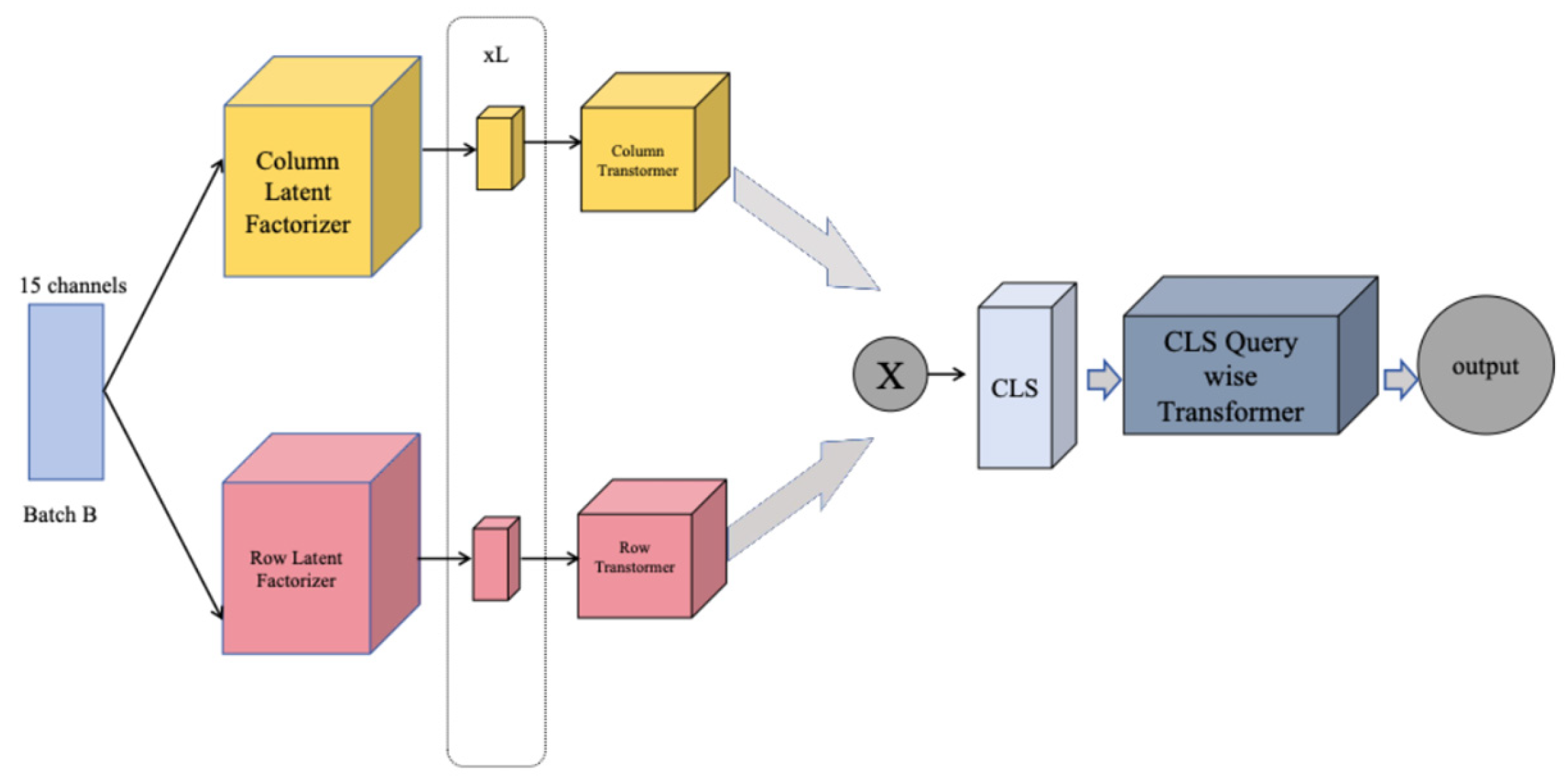
The LF-Transformer is a deep learning model designed for high-dimensional data with strong spatiotemporal correlations. Compared with traditional machine learning methods such as Random Forest, it demonstrates significantly enhanced modeling capabilities. While Random Forest is suitable for structured tabular data, it struggles with the complex spatiotemporal structures present in remote sensing images or meteorological data. The LF-Transformer, based on the Transformer architecture, incorporates multiple structural innovations to better handle unstructured, multi-channel, and complex data modeling tasks. The model architecture is shown in Figure 1. As shown in Figure 1, the LF-Transformer follows a structured and directional information flow. The input consists of multi-channel satellite observations, which are first processed by two parallel latent factorization pathways: the column latent factorizer and the row latent factorizer. These two modules reorganize the input features along the channel-wise and instance-wise directions, respectively, enabling the extraction of complementary directional representations. The factorized latent tokens are then fed into the corresponding column-wise and row-wise Transformer encoders to model long-range dependencies. The outputs of the two branches are subsequently fused through an interaction module, and the fused representation is finally summarized by a CLS query-wise Transformer to produce the visibility classification output.

2.1.2. Row/Column Factorization Mechanism

As illustrated in the left part of Figure 1, the row/column latent factorization mechanism decomposes the input feature space along orthogonal directions before Transformer encoding. To better capture directional features in remote sensing or temporal data, the LF-Transformer introduces a row/column factorization mechanism. Since the input in this study consists of station-matched, channel-based tabular data, this factorization can also be regarded as a structured decomposition of the multispectral feature dimensions, enabling the model to more effectively capture the physical response differences among spectral channels. By serializing the input tensor independently along the row and column directions, the model can extract orthogonal directional features. Compared with applying attention directly to a 2D feature map, this design enhances the model’s expressive capacity, reduces computational complexity, and improves its awareness of directional structural patterns.

Following the formulation of the latent factorizer in the original LF-Transformer, each input feature is first embedded into a shared latent space. Given the $j$-th input feature $x_j$, its token embedding is defined as $T_j=b_j+f_j\left(x_j\right), f_j:X_j\to R^d$, where $b_j$ denotes a learnable bias term and $f_j$ represents the feature-specific embedding function. For numerical features, the embedding function is implemented as an element-wise scaling with a learnable weight vector, ${ T}_j^{\left(num\right)}=b_j^{\left(num\right)}+x_j^{\left(num\right)}{W}_j^{\left(num\right)}$ while categorical features are embedded via a lookup table, ${ T}_j^{\left(cat\right)}=b_j^{\left(cat\right)}+e_j^T{W}_j^{\left(cat\right)}$, where $e_j^T$ denotes the corresponding categorical embedding. To enable latent-space aggregation, a set of learnable latent factor tokens $F\in R^{p\times d}$ is prepended to the feature token sequence. The resulting embedding matrix is then constructed as $T=stack\left[F,T_1^{\left(num\right)},\dots ,T_{k^{\left(num\right)}}^{\left(num\right)},T_1^{\left(cat\right)},\dots ,T_{k^{\left(cat\right)}}^{\left(cat\right)}\right]T\in R^{(k+p)\times d},F\in R^{p\times d}$, where $p$ is the dimension of the latent factor and $k$ represents the total number of input features. In this study, these latent factor tokens act as abstract information aggregation slots, enabling the subsequent row-wise and column-wise Transformer layers to summarize, denoise, and reorganize feature information within a compact latent space. This factorized token representation forms the foundation for directional encoding in the following row and column Transformer modules.

2.1.3. Row/Column Transformer Encoding Modules

Corresponding to the Column Transformer and Row Transformer blocks shown in Figure 1, the LF-Transformer applies two parallel Transformer encoders to capture long-range dependencies along the channel and instance dimensions. Building on the factorization step, the LF-Transformer further incorporates Row Transformer and Column Transformer modules to encode sequences along both directions and capture long-range dependencies. For tabular multispectral remote-sensing data, such row/column encoding is particularly effective in modeling long-range cross-channel relationships, such as the heterogeneous spectral responses associated with surface temperature variations and low-level water vapor content. This dual-path structure not only increases modeling flexibility but also makes the model better suited for analyzing directional or banded patterns in remote-sensing observations—such as wind fields or cloud bands—while remaining more computationally efficient than standard Transformer architectures.

In this study, the column-wise Transformer operates along the feature/channel dimension, whereas the row-wise Transformer operates along the instance dimension constructed by re-organizing the input tensor (e.g., across stations or temporal samples). Both Transformers adopt a PreNorm architecture, and in the final encoding layer, only the latent factor tokens are used as queries to aggregate information from all tokens. This query-wise design significantly reduces computational cost while retaining the most informative directional representations.

2.1.4. Interaction Fusion Module

As depicted in the central fusion stage of Figure 1, the representations generated by the row-wise and column-wise Transformer branches are integrated through an interaction-fusion module. To integrate the representations produced by the two directional encoders, the LF-Transformer introduces an interaction-fusion module. Low-visibility conditions are typically driven by multiple factors acting together, such as the combination of high near-surface humidity + temperature inversion + weak wind conditions. A single processing pathway cannot adequately model the interactions among these components.

In this work, interaction fusion is implemented as a channel-wise bilinear outer-product operation between the latent factor representations generated by the row-wise and column-wise Transformers. Let $H^c\in R^{B\times f\times d}$ and $H^r\in R^{B_r\times f\times d}$ denote the latent factor outputs obtained from the final query-wise Transformer layer of the column and row branches, respectively, where $f$ is the number of latent factor tokens and $d$ is the embedding dimension. For each embedding channel $k$, an interaction map is computed as $Z_k=H_{:,:,k}^c{\left(H_{:,:,k}^r\right)}^T\in R^{B\times B_r}.$ Stacking all channels yields the fused representation $Z\in R^{B\times B_r\times d}$, which explicitly captures second-order interactions between row-wise and column-wise latent factors. The computational complexity of this fusion is $\mathcal{O}(d\cdot B\cdot f\cdot B_r)$, enabling efficient modeling of high-dimensional feature interactions without introducing quadratic complexity in the embedding dimension.

By explicitly constructing such interaction features, the LF-Transformer can effectively capture compound physical signals, such as the joint evolution of near-surface moisture accumulation and temperature stratification, which are critical for low-visibility formation.

2.1.5. CLS Decoding Module

As shown in the rightmost part of Figure 1, a CLS query-wise Transformer is employed to aggregate the fused interaction features for final visibility classification. The LF-Transformer employs a [CLS] token decoding mechanism, similar to that used in BERT, to extract discriminative information from the fused feature representation for classification tasks. Since changes in visibility are typically the result of multiple subspace signals acting together, the [CLS] token aggregates key information from water-vapor–sensitive channels, temperature channels, and cross-station structural features.

In particular, the final decoding stage adopts a CLS query-wise attention mechanism, where only the [CLS] token attends to all interaction tokens to summarize global discriminative cues. For example, prior to the formation of near-surface fog, the aggregated [CLS] representation can simultaneously capture signals such as rapid moisture accumulation, surface temperature drops, and weakening wind speeds—patterns that traditional Random Forest models cannot effectively encode. This deep semantic decoding mechanism enables the LF-Transformer to model more complex feature interactions, thereby improving both the accuracy and generalization capability of visibility classification.

In summary, the LF-Transformer enhances the standard Transformer architecture by introducing row/column factorization, parallel row/column Transformer encoding, interaction fusion, and a CLS decoder, which improve its ability to model data structures. It is particularly well suited for remote sensing and meteorological data with spatiotemporal structures, spatial relationships, or temporal evolution patterns. While Random Forest offers good interpretability and efficiency, it has clear limitations in feature representation, long-range dependency modeling, and capturing multi-dimensional interactions. When processing high-dimensional, multi-channel, temporal data, it cannot match the LF-Transformer. Therefore, the LF-Transformer not only overcomes the structural limitations of traditional methods but also demonstrates substantial advantages in handling complex data.

After systematically discussing the architectural advantages and deep feature modeling capabilities of the LF-Transformer in the previous section, we now extend the experimental comparison to evaluate the classification performance of the LF-Transformer, Random Forest, and Saint models on representative datasets. Among these baseline methods, Saint is a Transformer-based model specifically designed for tabular data, which enhances feature interaction modeling and sample-level representation learning through row-wise attention mechanisms and contrastive pre-training strategies, and has demonstrated strong performance across a wide range of structured data tasks [23]. This comparison highlights the adaptability and superiority of the LF-Transformer across different types and structures of data tasks. This section not only supports the theoretical arguments regarding the model’s structural advantages but also provides data-driven insights for practical applications.

2.2. Dataset Description

To ensure the scientific rigor and representativeness of model training and evaluation, this study constructed a fused dataset combining observations from Fengyun-4A and Fengyun-4B satellites (hereafter referred to as the FY4A+4B fused dataset), designed to support regional traffic meteorological warning tasks. Centered on the Jiaxing–Shaoxing Bridge (Jia-Shao Bridge), the dataset is built for regional traffic weather warning scenarios, encompassing multi-dimensional features in the temporal, spatial, and spectral domains, making it both representative and challenging. The specific data preparation process is as follows:

The FY4A+FY4B dataset is constructed based on geostationary satellite observations from Fengyun-4A (FY-4A) and Fengyun-4B (FY-4B). The raw data are sourced from the Level-1AGRI products (full-disk, 4 km resolution) publicly released by the National Satellite Meteorological Center (NSMC). Most visible/infrared channels have a typical spatial resolution of 4 km, while several high-resolution visible channels reach 0.5 km, 1 km, or 2 km. The satellites provide an observation temporal resolution of 15 min. The dataset can be accessed at: https://satellite.nsmc.org.cn/DataPortal/cn/data/detail.html (accessed on 29 July 2025). The dataset spans from January 2021 to December 2023, covering multiple typical low-visibility weather events and exhibiting clear seasonal and interannual variability. The detailed processing steps are as follows:

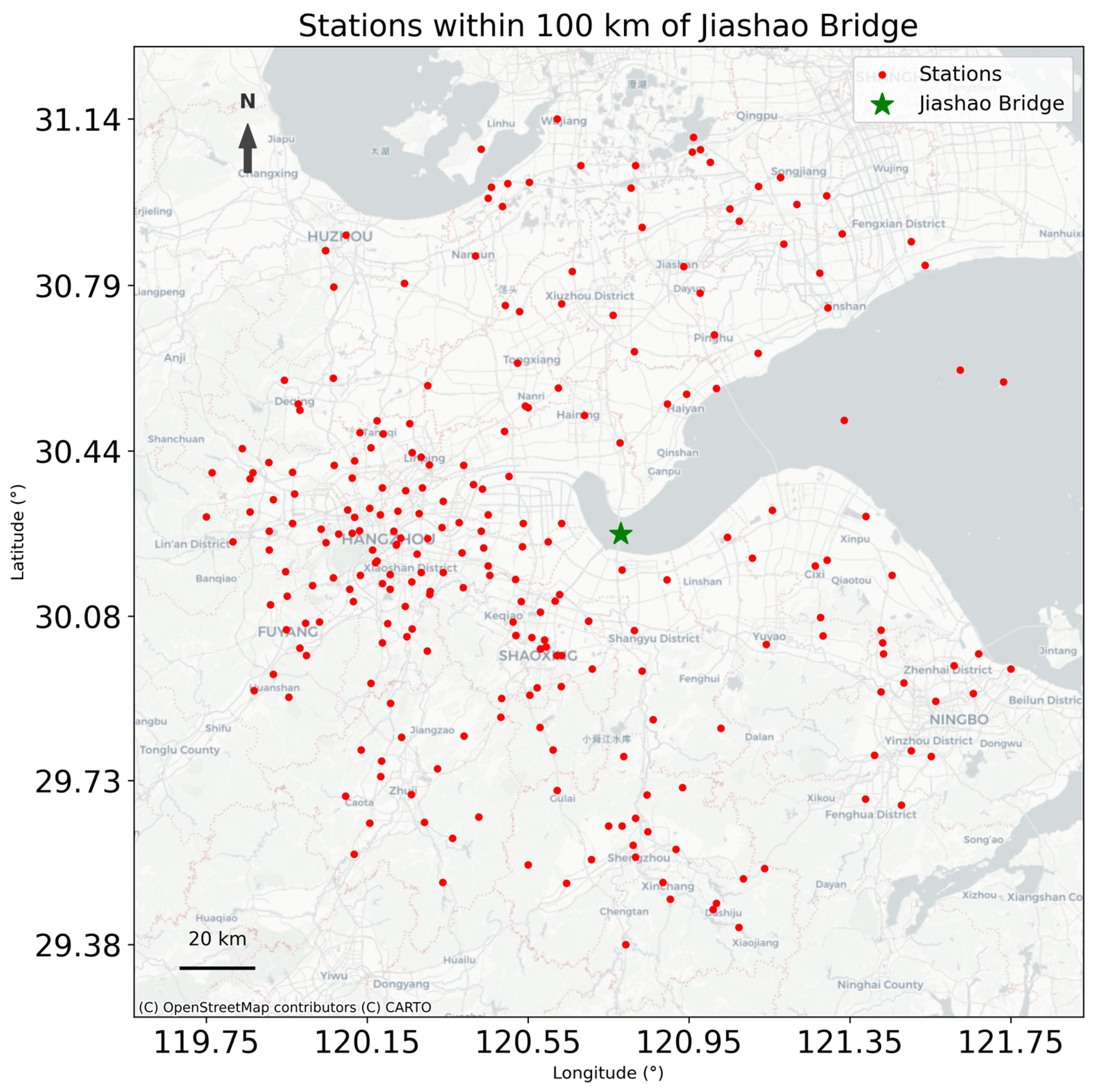
Spatial range definition: The study area is defined as a 10,000 km² region centered on the Jia-Shao Bridge, covering approximately 240 ground-based meteorological observation stations. Stations with altitudes exceeding 500 m were excluded, as well as anomalous stations with more than 900 observation records in the historical dataset, to ensure data quality and representativeness (as shown in Figure 2).

Feature extraction: For each station, radiance or brightness temperature data from 15 infrared and visible channels provided by the FY4A and FY4B satellites were extracted as basic input features.

Label construction: Finally, according to the visibility observations matched with the corresponding remote sensing timestamps, each sample was categorized into four visibility levels, as shown in

Table 1. Grades of Fog Forecasting.

Visibility Level (Class)	Visibility Range (m)	Corresponding Weather Condition
Class 0	0–200	Dense fog or thick fog
Class 1	201–500	Heavy fog
Class 2	501–1000	Moderate fog
Class 3	>1000	Clear weather without fog or haze

. The classification follows the national standard “Grades of Fog Forecasting” (GB/T 27964-2011) issued by the China Meteorological Administration and is further adjusted to align with the practical requirements of transportation meteorological services [24].

This dataset is primarily designed to evaluate the model’s ability to classify visibility levels based on satellite channel data. It integrates synchronous observations from two geostationary meteorological satellites, providing strong temporal continuity, high channel diversity, extensive spectral coverage, and complex spatiotemporal structures. The dataset construction process includes the following steps:

(1) Spatiotemporal registration:

First, spatial and temporal registration was performed on the satellite observation data from Fengyun4A (FY4A) and Fengyun4B (FY4B). Since the two satellites have slight differences in orbital positions and viewing angles, a lookup table (LUT)-based geographic coordinate mapping and time alignment mechanism was applied to ensure that the data from both satellites correspond precisely to the same ground sites and observation times.

(2) Channel matching and fusion strategy:

Compared with FY-4A, FY-4B includes an additional low-level water vapor channel with a central wavelength of 7.42 μm. This channel is designed to detect lower-tropospheric water vapor content (especially from the boundary layer to the lower troposphere). Low-level water vapor is the “raw material” for precipitation and directly affects boundary-layer temperature, cloud-base height, and turbulent exchange—making it a key parameter for weather forecasting (e.g., heavy rain or fog prediction) and climate research. Although FY4A also contains several water vapor channels (e.g., 6.25 μm and 7.1 μm), the 7.42 μm band is closer to the water vapor absorption peak and thus provides higher accuracy in detecting low-level water vapor.

The specific processing method is as follows: for the 14 channels shared by both satellites, a one-to-one mapping is performed, and their original physical features are retained as inputs. For the FY-4B-specific 7.42 μm low-level water vapor channel, this study explicitly adopts direct concatenation as an additional input dimension. To maintain consistent input dimensionality, an empty placeholder channel (filled with zero values) is added to the FY-4A dataset. This placeholder does not carry any physical information and therefore does not alter the structure of FY-4A data or affect model learning. This strategy enables the use of the additional FY-4B channel without disrupting the overall input structure. Ultimately, a 15-dimensional channel feature input is formed—one dimension higher than FY-4A alone—while preserving the physical meaning of all existing channels.

(3) Feature enhancement:

Derived features such as spatiotemporal differences and spectral ratios were constructed through cross-channel operations to provide the model with richer spatially heterogeneous information.

(4) Label consistency assurance:

Visibility observations from the FY4A+FY4B fused dataset were used as classification labels to ensure that while the model input space was expanded, the supervision signal remained consistent.

This fused dataset significantly expands the feature dimensionality, offering stronger inter-channel complementarity and higher spatiotemporal complexity. It imposes greater demands on the model’s structural modeling capability and more closely reflects real-world multi-source remote sensing fusion applications.

After constructing the FY4A+FY4B fused dataset, this study adopts a hold-out validation strategy, dividing all samples into training, validation, and test sets with a ratio of 8:1:1. Unlike K-fold cross-validation, the hold-out method reduces the computational cost while ensuring sufficient sample size. The LF-Transformer, Random Forest, and Saint models are trained and evaluated on the same data partitions, thereby guaranteeing fairness and reproducibility in the model comparison.

Given the pronounced imbalance in the original visibility-level distribution, particularly the dominance of Class 3 samples, stratified sampling was first applied during data partitioning to ensure consistent proportional distributions of the four visibility classes across the training, validation, and test sets. On this basis, to further enhance the model’s ability to learn low-frequency classes (Class 0–2) and to mitigate bias toward the majority class, a resampling strategy was introduced during dataset construction, such that each visibility level in the test set used for model evaluation contained an equal number of samples. Specifically, each visibility class in the test set comprised 700 samples. This design effectively strengthens the model’s sensitivity and generalization ability for minority classes and prevents performance bias caused by class imbalance.

It should be emphasized that fog events in real-world environments inherently exhibit a highly imbalanced distribution. To better reflect operational conditions, several naturally occurring days of observations were additionally selected as an independent test set during the evaluation stage. In contrast to the balanced samples constructed for model training, this test set retains the original, naturally imbalanced distribution of visibility levels, thereby providing a more realistic characterization of fog occurrence. Accordingly, the performance evaluation of the model is conducted on this naturally imbalanced dataset, ensuring that the resulting assessment is more representative, interpretable, and aligned with practical application requirements.

2.3. Evaluation Metrics and Model Training

To systematically evaluate the visibility classification capability of LF-Transformer, Random Forest, and Saint under the same data conditions, this study conducts experiments using the FY4A+FY4B satellite fused dataset. Precision, Recall, and F1-score are employed as model performance evaluation metrics, and their calculation formulas are shown in Equations (1)–(3).

Here, TP (True Positive) represents the number of samples correctly classified into the target category by the model; FP (False Positive) represents the number of samples incorrectly classified into the target category; FN (False Negative) represents the number of samples that belong to the target category but were misclassified into other categories. P (Precision) reflects the accuracy of the model’s predictions, R (Recall) reflects the model’s ability to identify samples of a specific class, and F1 (F1-score) is the harmonic mean of precision and recall, providing a comprehensive measure of classification performance.

$$P={\displaystyle \frac{TP}{TP+FP}}\times 100\%$$

(1)

$$R={\displaystyle \frac{TP}{TP+FN}}\times 100\%$$

(2)

$$F1={\displaystyle \frac{2\times P\times R}{P+R}}\times 100\%$$

(3)

After defining the evaluation metrics, we further provided a systematic description of the training procedures, hyperparameter configurations, and metric computation methods to ensure a fair comparison among the LF-Transformer, Random Forest, and Saint models under identical conditions.

First, the LF-Transformer was trained in an end-to-end manner. The training process employed the Adamw optimizer with an initial learning rate of 2.67 × 10⁻⁵, which was adaptively adjusted using a cosine annealing strategy. The training batch size was set to 50, and the evaluation batch size was also set to 50. A weighted cross-entropy loss function was used to alleviate training bias caused by class imbalance among visibility levels. An Early Stopping mechanism with a patience of 16 was applied, monitoring the Macro-F1 score on the validation set to prevent overfitting. To further enhance training stability, the parameters were initialized using Kaiming initialization; input features were normalized using Quantile Normalization, and categorical features were encoded using the “indices” scheme. All hyperparameter settings were determined based on validation performance to ensure stability and generalization capability when processing multi-channel remote sensing data.

Second, to ensure fairness in comparison, the key hyperparameters of the Random Forest model were carefully tuned. The Random Forest Classifier from Sklenar was used as the baseline model, with explicit settings for important hyperparameters. Specifically, the number of trees was set to 100, and the maximum depth was set to None to allow each decision tree to fully grow. The feature selection strategy followed the Sklenar default of “sqrt”. The minimum number of samples required to split an internal node was set to 2, and the minimum number of samples required at a leaf node was set to 1. To mitigate the effects of class imbalance in visibility levels, class weight was set to “balanced”, and random state was fixed at 42 to ensure reproducibility. All remaining parameters followed Sklenar defaults, including using the Gini index (criterion = “gini”) as the splitting criterion and enabling bootstrap sampling for constructing each decision tree.

To further expand the model comparison and comprehensively evaluate the performance of different deep learning architectures on the multi-channel remote sensing visibility classification task, this study introduces the Saint (Self-Attention and Intersample Attention Transformer) model as a third benchmark model. The Saint architecture adopts a standard Transformer encoder while integrating an intersample attention mechanism, which strengthens the modeling of relationships across samples and enhances its capability to capture complex patterns within multi-channel remote sensing features.

In terms of training configuration, the key hyperparameters of Saint—including optimizer selection, learning rate, and weight-decay settings are aligned with those of the LF-Transformer to ensure fairness and reproducibility in cross-model comparison. Specifically, the model is trained using the Adamw optimizer and incorporates the same learning rate scheduling and regularization strategies as the LF-Transformer. An Early Stopping mechanism (patience = 16), monitoring the Macro-F1 score on the validation set, is also applied to prevent overfitting. Regarding structural hyperparameters, the Transformer depth, number of attention heads, and dropout settings of the Saint model are determined through performance tuning based on the validation set. Overall, the Saint model is fully aligned with the LF-Transformer in terms of training procedure, optimization strategy, and validation mechanism, thereby ensuring that all three models are compared fairly under a unified data setting and training framework.

Regarding the model validation strategy, only the training set was used for parameter updates during the training phase; the validation set was used to monitor validation metrics and apply early stopping; and the test set was used exclusively for final performance evaluation. All three models—LF-Transformer, Random Forest, and Saint were trained and tested using an identical train/validation/test split to ensure comparability and reproducibility of results.

Finally, all evaluation metrics—including Precision, Recall, and F1-score (computed according to Equations (1)–(3)) were calculated on the independent test set to ensure the independence and objectivity of the evaluation outcomes. Next, we compare the performance differences among the three models across different categories and further analyze their adaptability and modeling capability for multi-channel remote sensing data.

3. Experiments and Results

3.1. Experimental Comparison

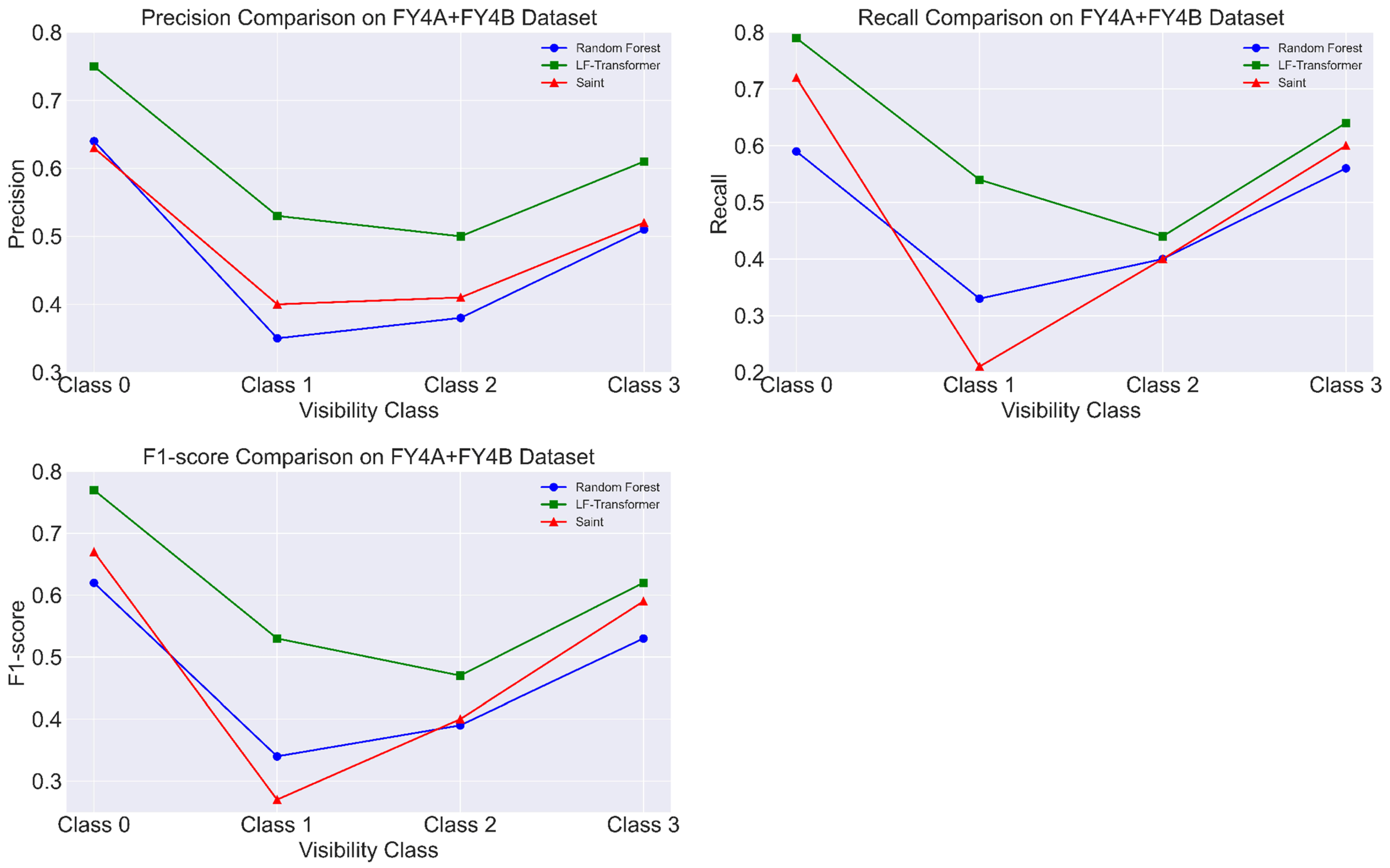
In the systematic evaluation of classification performance on the FY4A+FY4B fused dataset, we first summarized the Precision, Recall, and F1-score values of LF-Transformer, Random Forest, and Saint across the four visibility levels and compiled them into a performance comparison table, as shown in

Table 2. Performance Comparison of LF-Transformer, Random Forest, and Saint on the FY4A+FY4B Dataset.

FY4A+FY4B
	Precision			Recall			F1-Score
	LF	RF	Saint	LF	RF	Saint	LF	RF	Saint
0	0.75	0.64	0.60	0.79	0.59	0.72	0.77	0.62	0.67
1	0.53	0.35	0.40	0.54	0.33	0.21	0.53	0.34	0.27
2	0.50	0.38	0.41	0.44	0.40	0.40	0.47	0.39	0.40
3	0.60	0.51	0.52	0.64	0.56	0.60	0.62	0.53	0.59

. This table provides a quantitative foundation for the subsequent analysis and makes the differences among the three models across various metrics and categories more explicit. On this basis, we further plotted the line charts of Precision, Recall, and F1-score to illustrate the performance variation and overall trends of LF-Transformer, Random Forest, and Saint across different visibility levels, as shown in Figure 3.

Figure 3 compares the classification performance of LF-Transformer, Saint, and Random Forest on the FY4A+FY4B fused dataset, covering three core evaluation metrics: Precision, Recall, and F1-score. Overall, LF-Transformer significantly outperforms the other two models across all visibility categories and all metrics, while the performance of Saint falls between LF-Transformer and Random Forest.

Taking the F1-score as an example, LF-Transformer achieves an average score of 0.59 across the four categories, representing an increase of approximately 13% over the value of 0.47 obtained by Random Forest and also exceeding the value of 0.48 achieved by Saint. LF-Transformer maintains a high recall while effectively controlling the false-positive rate, demonstrating a more desirable balance between precision and recall. In contrast, although Saint performs similarly to LF-Transformer in Class 0 and Class 3, its F1-score drops sharply to 0.27 in Class 1, indicating that it still struggles to recognize intermediate visibility levels.

For Precision and Recall, the LF-Transformer achieves average values of 0.59 and 0.60, respectively, which are markedly higher than the values of 0.47 obtained by Random Forest and also superior to the value of 0.48 achieved by Saint. Moreover, LF-Transformer exhibits smaller variations across categories (standard deviations of 0.10 and 0.11 for Precision and Recall, respectively; compared with 0.13 and 0.12 for Random Forest, and 0.10 and 0.20 for Saint), suggesting stronger robustness and adaptability under complex or extreme conditions.

This performance advantage is particularly critical for visibility-level classification. Due to the continuity and fuzzy boundaries between visibility levels, traditional methods often struggle in transition regions. By leveraging deep feature modeling and multi-source information fusion, LF-Transformer shows enhanced adaptability and recognition ability when dealing with complex and ambiguous scenarios. Meanwhile, Saint outperforms Random Forest in most categories, further indicating that Transformer-based architectures are more suitable for high-dimensional, multi-channel remote-sensing visibility retrieval tasks.

In summary, the results in Figure 3 provide a clear and systematic demonstration of the performance superiority of LF-Transformer, offering strong support for its practical application and broader adoption in remote-sensing-based visibility classification.

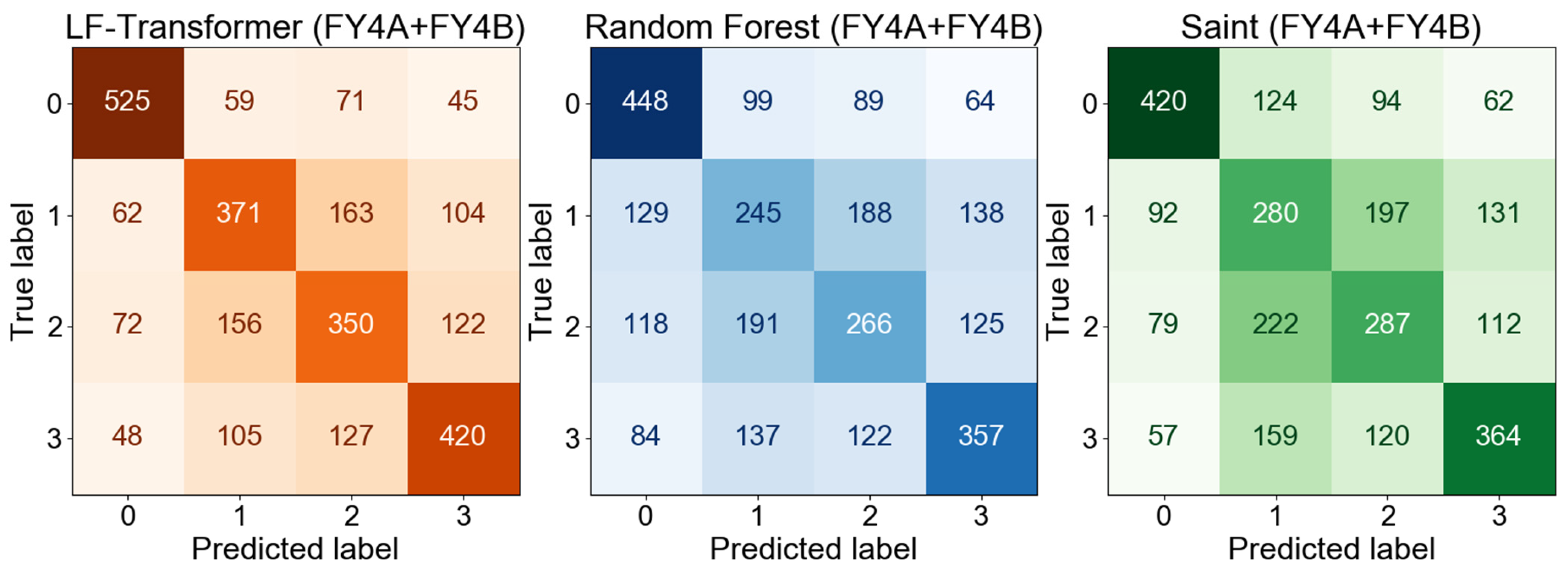
To further reveal the prediction distribution and misclassification patterns of each model across different categories, Figure 4 presents the visualized confusion matrices of the three models. These matrices intuitively reflect the prediction distribution for each class and provide useful insight into overall classification performance.

Overall, the LF-Transformer shows noticeably higher values along the main diagonal compared with both Random Forest and Saint, indicating its stronger ability in correct classification. For example, in the dense or thick fog category (Class 0), the LF-Transformer correctly identified 525 out of 700 samples, achieving a precision of 75%, which is 11% higher than Random Forest and also superior to Saint’s 420 correctly identified samples. In addition, LF-Transformer produced fewer false positives in non-target categories, demonstrating its superior capability in recognizing low-visibility conditions. Although Saint performs significantly better than Random Forest in this class, it still falls slightly behind the LF-Transformer.

In the most challenging heavy fog category (Class 1), the LF-Transformer correctly classified 371 out of 700 samples, reaching a precision of 53%, which is 8% higher than the 245 correctly identified samples of Random Forest. Most of its misclassifications were concentrated in the adjacent categories (Class 0 and Class 2), indicating fewer random errors and better interpretability. In contrast, Saint performed relatively poorly in Class 1, correctly identifying only 280 samples, with more dispersed misclassification patterns. This suggests that it still struggles to handle the fuzzy boundaries characteristic of intermediate low-visibility levels.

In the moderate fog (Class 2) and clear weather (Class 3) categories, the LF-Transformer again demonstrates higher precision and more concentrated misclassification patterns. Compared with Random Forest, it achieves performance improvements across all categories. Saint performs similarly to or slightly better than Random Forest in these two classes (e.g., 420 correct predictions in Class 3), but overall, it remains inferior to the LF-Transformer, reflecting differences in the ability of Transformer-based architectures to model samples with fuzzy category boundaries.

In summary, the LF-Transformer provides more stable and accurate class discrimination and shows significant advantages and strong application potential under complex meteorological conditions. Saint performs better overall than Random Forest but still requires improvement in the more difficult classification categories.

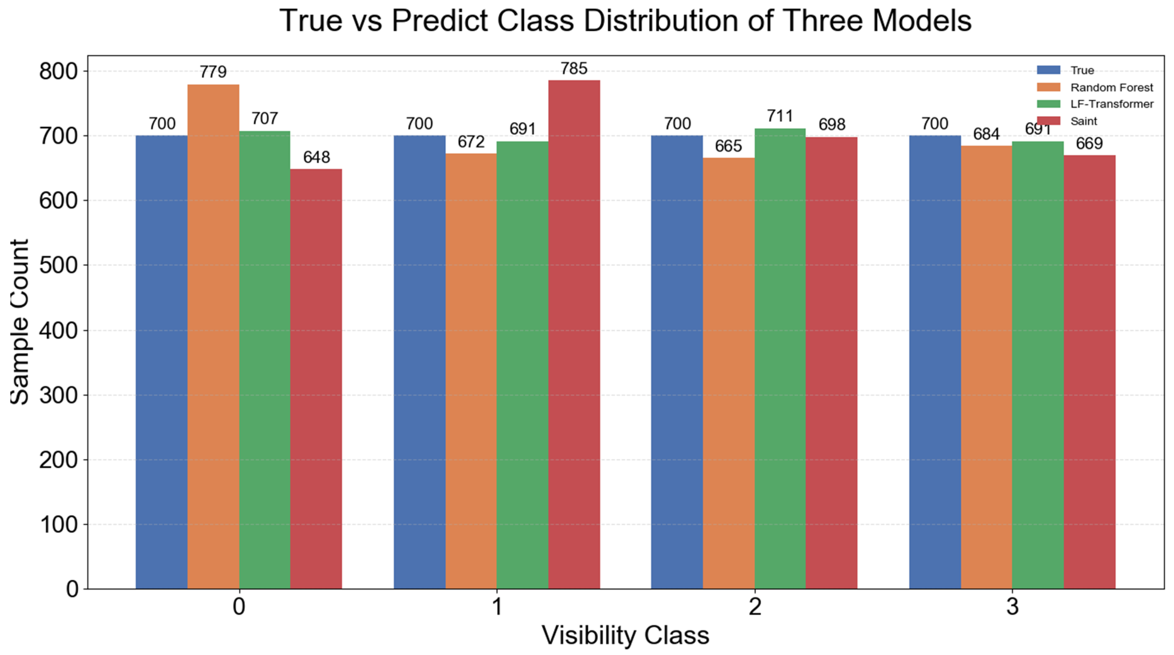
To more intuitively analyze the prediction tendencies and misclassification distributions of the models across different categories, Figure 5 presents a comparison between the predicted results and the true labels for the Random Forest, LF-Transformer, and Saint models. The side-by-side bar charts show the differences in predicted sample counts for each class, a columnar summation in Figure 4, reflecting the degree of classification bias exhibited by each model.

Overall, the LF-Transformer’s predictions are closer to the true distribution. It slightly overestimates the dense or thick fog (Class 0) and moderate fog (Class 2) categories, while slightly underestimating the heavy fog (Class 1) and clear weather (Class 3) categories. However, the model shows a minimum-bias in Class 1 and Class 3, compared to the other two methods, suggesting the reliability of its discrimination between frog and non-frog events. Also, because its predictions are more concentrated, the model appears to effectively capture inter-class feature boundaries, demonstrating LF-Transformer’s advantages in maintaining classification consistency and controlling misclassification.

In contrast, the Random Forest model shows significant underestimation and dispersed predictions in the heavy fog (Class 1) and moderate fog (Class 2) categories, consistent with the instability observed in its confusion matrix.

The Saint model also exhibits notable prediction bias. It overestimates Class 1, with the predicted sample count reaching 785, while underestimating Class 0 and Class 3, yielding only 648 and 669 samples, respectively, compared with the true count of 700. Although Saint’s predicted count for Class 2 is close to the true value, the confusion matrix in Figure 4 shows that its true positives are not high, indicating insufficient prediction concentration and stronger class confusion.

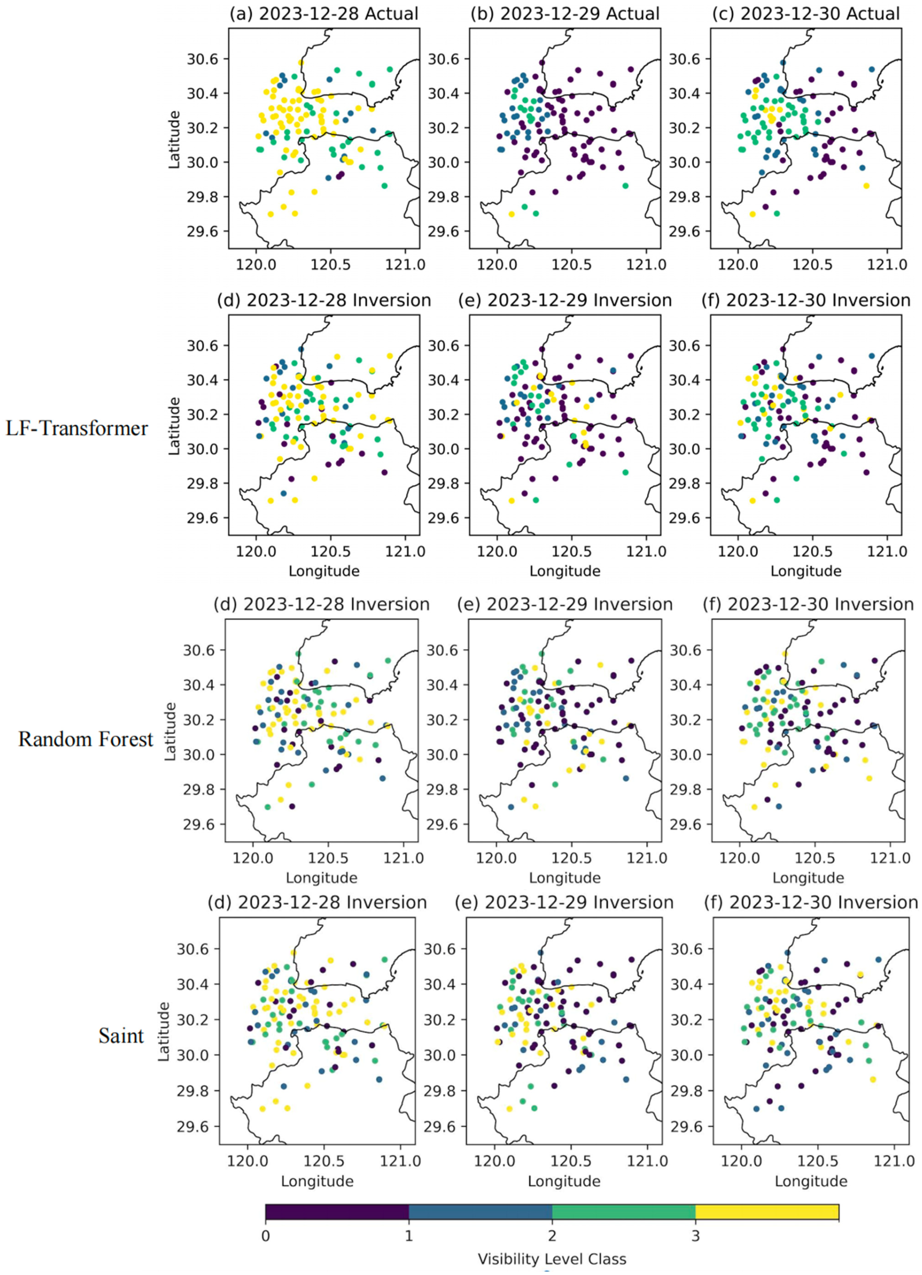
To further validate the practical inversion capabilities of the three models under low-visibility conditions, this study selected a typical persistent low-visibility event that occurred near the Jiaxing–Shaoxing Bridge in Zhejiang Province on 28–30 December 2023, and visualized the predicted visibility levels at observation stations, as shown in Figure 6. The color shading in the figures represents different visibility classes.

As shown in Figure 6, the LF-Transformer can well reproduce the horizontal distribution patterns and intensity inversion characteristics observed in real conditions. Specifically, the model exhibits the highest stability in identifying dense or thick fog areas (Class 0), with a misclassification rate of only 27%. The misclassification rate for clear-weather conditions without fog or haze (Class 3) is 35%, while the rates for heavy fog (Class 1) and moderate fog (Class 2) are 46% and 52%, respectively.

These differences may be related to the varying complexity of observational features corresponding to different visibility levels. Dense or thick fog (Class 0) typically exhibits more pronounced radiative characteristics (such as strong absorption signals in the 7.42 μm low-level water vapor channel), making it easier for the model to capture its spatial distribution. In contrast, heavy fog (Class 1) and moderate fog (Class 2) exhibit weaker radiative differences from their surroundings and have more ambiguous boundaries, leading to confusion between adjacent levels.

Compared with the LF-Transformer, the spatial inversion results of the Random Forest model reveal significantly weaker recognition capability in low-visibility regions, with reconstructed spatial structures deviating substantially from the observed distribution. Specifically, the Random Forest shows unstable performance in identifying dense or thick fog (Class 0), with a misclassification rate of 38%, and incorrectly classifies large portions of the core low-visibility region as Class 1 or Class 2, resulting in pronounced omission errors. For heavy fog (Class 1) and moderate fog (Class 2), the Random Forest’s misclassification rates reach 60% and 58%, respectively—substantially higher than those of the LF-Transformer. Its spatial predictions exhibit clear over-smoothing, blurred fog boundaries, inaccurate intensity gradients, and even cross-regional misclassification, indicating limited capability in distinguishing mid-level fog features. Under clear-weather conditions (Class 3), although the Random Forest can roughly capture the large-scale structure of non-fog areas, its misclassification rate remains as high as 45%.

The Saint model demonstrates spatial inversion accuracy between that of the LF-Transformer and Random Forest. Its misclassification rates for Class 0, Class 1, Class 2, and Class 3 are 42%, 56%, 60%, and 43%, respectively. Saint performs better than Random Forest in identifying dense fog (Class 0) but still falls noticeably short of the LF-Transformer, with local fog boundaries remaining blurred. For heavy fog (Class 1) and moderate fog (Class 2), Saint’s misclassification rates are comparable to those of the Random Forest, showing substantial spatial confusion and cross-regional errors, especially in mid-level fog regions where it struggles to capture fine-scale structures. In clear-weather conditions (Class 3), Saint can stably identify large-scale non-fog areas, but still exhibits a non-negligible proportion of misclassification, failing to match the spatial consistency achieved by the LF-Transformer.

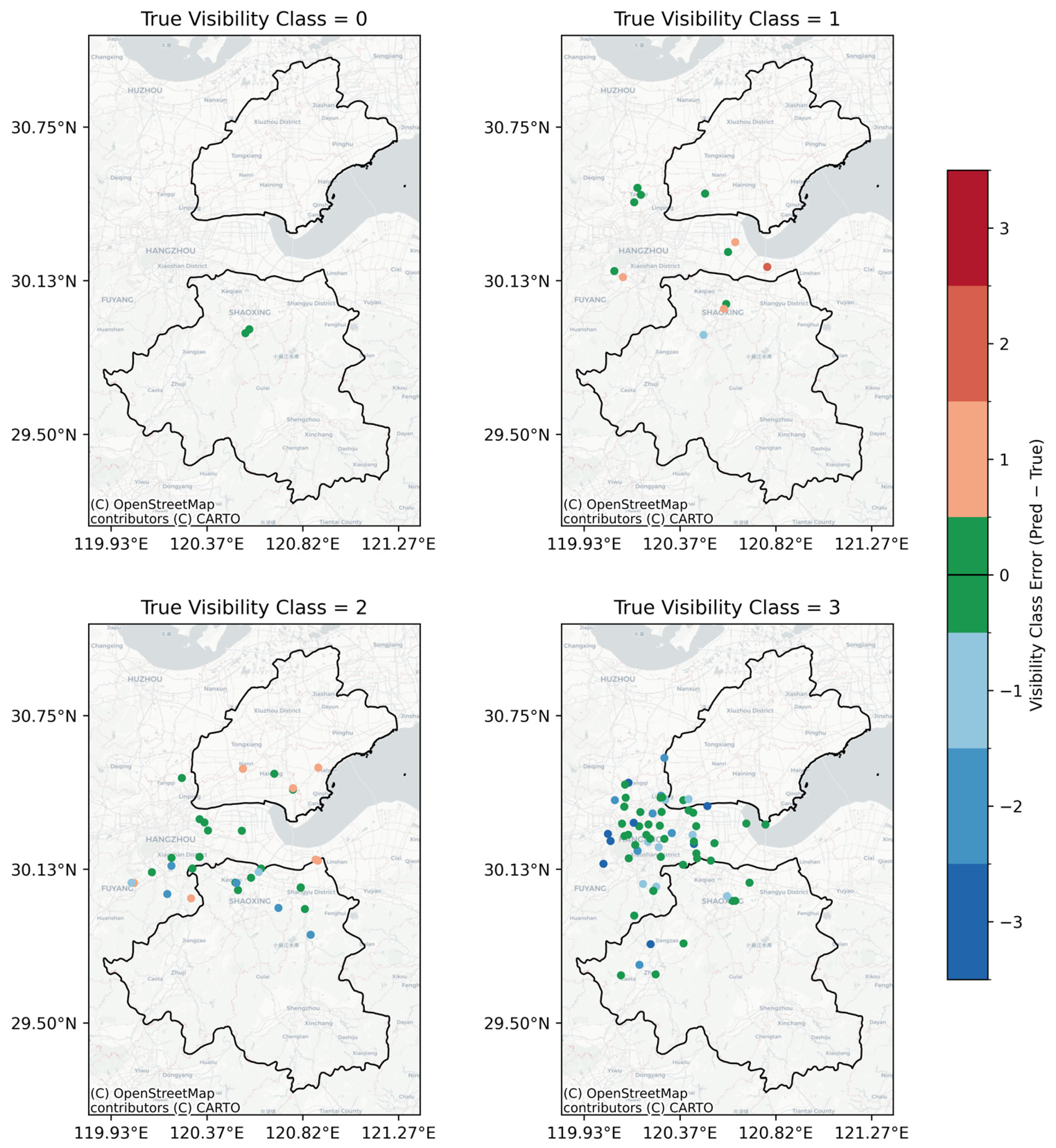
To characterize the prediction bias of different models across various visibility levels, the spatial distribution of prediction errors at observation stations was analyzed for a representative Zhejiang low-visibility event on 28 December 2023. Figure 7 presents the spatial error distribution produced by the LF-Transformer model, while the corresponding results for the Random Forest and Saint models are provided in Supplementary Figures S1 and S2, respectively. The prediction error is defined as the difference between the predicted visibility class and the true visibility class (Predicted Class−True Class). An error value of zero indicates a correct prediction, while positive and negative values indicate overestimation and underestimation of the visibility level, respectively.

As shown in Figure 7, the LF-Transformer exhibits relatively small prediction errors across all true visibility classes, with a high degree of spatial consistency. Under dense or thick fog (Class 0) and heavy fog (Class 1) conditions, prediction errors are mainly concentrated around zero, with only localized deviations between adjacent visibility classes, indicating strong prediction stability under low-visibility conditions.

For moderate fog conditions (Class 2), prediction errors increase to some extent; however, the spatial distribution remains relatively continuous, suggesting that the LF-Transformer maintains stable discrimination capability under transitional visibility levels. Under clear-weather conditions (Class 3), the error distribution is generally concentrated, demonstrating reliable performance in identifying high-visibility regions.

In contrast, the Random Forest model shown in Supplementary Figure S1 exhibits pronounced spatial dispersion in prediction errors. Under low-visibility conditions (Class 0–1), predictions at several stations within core low-visibility regions tend to shift toward higher visibility classes, resulting in an underrepresentation of low-visibility extent.

Under moderate fog conditions (Class 2), the Random Forest displays the most scattered error distribution, with fragmented spatial structures, indicating substantial uncertainty in distinguishing adjacent visibility classes. Even under clear-weather conditions (Class 3), a noticeable proportion of prediction bias remains, reflecting limited prediction stability under complex spatial patterns.

Supplementary Figure S2 presents the spatial distribution of prediction errors for the Saint model, whose overall performance lies between that of the LF-Transformer and the Random Forest. Under dense fog conditions (Class 0), Saint shows slight improvement compared to the Random Forest; however, error points still exhibit evident spatial dispersion.

Under heavy and moderate fog conditions (Class 1–2), the Saint model shows scattered error distributions with localized instability. For clear-weather conditions (Class 3), Saint can identify large-scale high-visibility regions, but the concentration of prediction errors remains weaker than that of the LF-Transformer.

Taken together, the comparison of prediction error distributions in Figure 7 indicates that the LF-Transformer produces more concentrated errors with greater spatial continuity and stability across all visibility classes. In contrast, the Random Forest and Saint models are more prone to dispersed prediction errors and fragmented spatial structures, particularly under moderate visibility conditions.

Overall, the LF-Transformer demonstrates superior performance not only in quantitative evaluation metrics but also in spatial consistency, showing stronger representational capability and more reliable inversion performance for regional fog recognition and early-warning applications. Saint outperforms Random Forest but still shows clear limitations in distinguishing complex fog structures and capturing fog boundaries.

3.2. Data Combination Comparison

To evaluate the benefits of multi-source remote sensing data fusion for low-visibility prediction, this study tested the LF-Transformer model on both the single-satellite FY4A dataset and the FY4A+FY4B fused dataset. The data comparison, summarized in

Table 3. Experimental Results of LF-Transformer on Different Datasets.

Class	Precision		Recall		F1-Score
	FY4A	FY4A+FY4B	FY4A	FY4A+FY4B	FY4A	FY4A+FY4B
Class 0	0.58	0.75	0.61	0.79	0.59	0.77
Class 1	0.42	0.53	0.24	0.54	0.30	0.53
Class 2	0.39	0.50	0.56	0.44	0.46	0.47
Class 3	0.52	0.61	0.48	0.64	0.50	0.62

, shows that data fusion significantly enhances the model’s discriminative ability across all visibility classes, particularly under low-visibility conditions. The global F1-score increased from 0.47 (weighted average) on the FY4A single-satellite dataset to 0.59 on the fused dataset, representing a 25.5% improvement.

Specifically, the most notable improvements were observed in dense or thick fog (Class 0), heavy fog (Class 1), and clear weather without fog or haze (Class 3):For Class 0, the F1-score increased from 0.59 to 0.77, Recall from 0.61 to 0.79, and Precision from 0.58 to 0.75, reflecting a significantly enhanced ability to discriminate extremely low-visibility scenarios. For Class 1, the F1-score rose from 0.30 to 0.53, Recall from 0.24 to 0.54, and Precision from 0.42 to 0.53. This improvement benefits from the complementarity of FY4A’s high-frequency sequences and FY4B’s global water vapor channels (e.g., 7.42 μm low-level water vapor), enabling the model to more sensitively detect early signals of visibility decline caused by rising humidity. For Class 3, the F1-score increased from 0.50 to 0.62, with Precision and Recall improving by 17% and 33%, respectively, indicating substantially higher accuracy in identifying excellent visibility conditions.

The complementary orbital design and observation timing of FY-4A and FY-4B provide richer spectral information and spatial resolution. Leveraging its self-attention mechanism and positional encoding, the LF-Transformer effectively integrates critical features across different channels and temporal slices, enabling cross-channel and cross-temporal information fusion. As a result, the model maintains or even improves classification performance under the increased data dimensionality afforded by multi-source fusion.

3.3. Interpretability Analysis Based on SHAP Values

Although deep learning-based prediction models demonstrate exceptional advantages in handling multi-source satellite data—owing to their strong nonlinear fitting capacity and ability to fuse spatiotemporal features—their “black-box” nature poses a major challenge in meteorological and environmental applications. The decision-making process of such models is buried within the complex nonlinear transformations of deep neural layers (e.g., the self-attention layers in Transformers or convolutional layers in CNNs). If the features driving low-visibility predictions deviate from established atmospheric physical mechanisms (for instance, mistakenly using vegetation indices as dominant predictors), the resulting predictions may lose physical interpretability and could even mislead operational decision-making (e.g., in hazard warning systems). Therefore, decomposing and explaining deep model behavior—verifying that its “black-box decisions” align with objective physical laws—is essential to ensure the model’s rationality, reliability, and operational value.

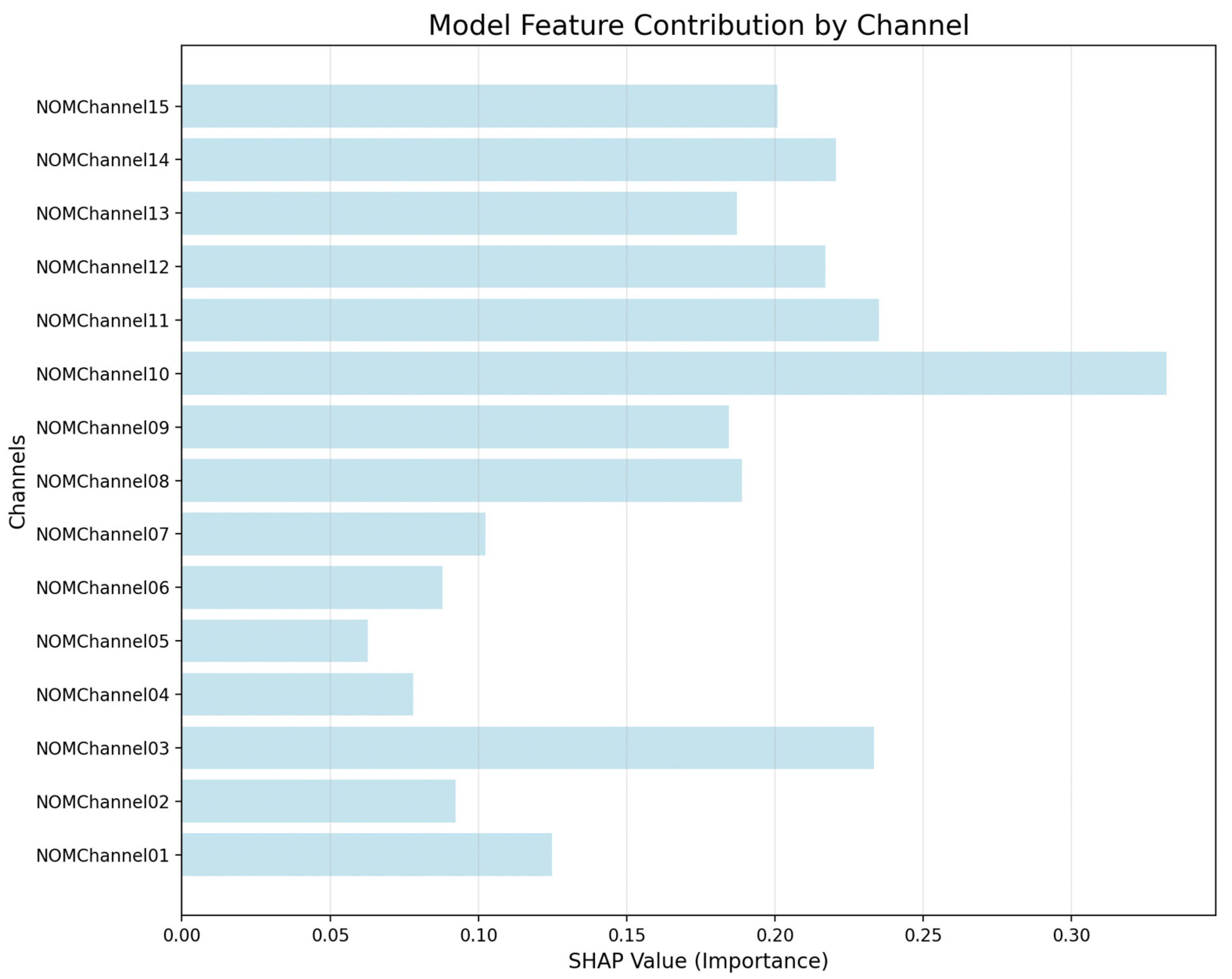
To analyze the LF-Transformer’s decision logic, this study employed DeepSHAP to quantify the marginal contributions of the 15 spectral channels, as illustrated in Figure 8. The SHAP value ranking of the channels aligns closely with atmospheric physical principles, clearly demonstrating the model’s ability to capture the core drivers of low-visibility conditions. Channels 10–15 and Channel 03 exhibit notably high SHAP values (most exceeding 0.2), with Channel 10 (SHAP = 0.33) being the highest. As shown in Supplementary Table S2, these channels are primarily associated with mid- to low-level water vapor characteristics, cloud features, and aerosol distributions over vegetation and water surfaces—indicating that variations in water vapor and cloud properties play a crucial role in near-surface fog and haze formation.

It is particularly noteworthy that Channel 11 (central wavelength 7.42 μm)—a new low-level water vapor channel unique to FY4B—has a SHAP value of 0.23 (ranked second), confirming its substantial contribution. However, SHAP values reflect relative importance under the learned model and do not directly quantify how much performance gain is attributable to a specific channel. Therefore, to further validate the physical interpretability and the practical contribution implied by SHAP, we conducted a controlled channel ablation experiment: the LF-Transformer was retrained and evaluated under identical settings, once removing the 7.42 μm channel (“Without 7.42 μm”) and once retaining it (“With 7.42 μm”). The results are reported in

Table 4. Performance comparison of the LF-Transformer on the FY-4A+FY-4B fused dataset with and without the 7.42 μm water vapor channel.

FY4A+FY4B
	Precision		Recall		F1-Score
	Without 7.42 μm	With 7.42 μm	Without 7.42 μm	With 7.42 μm	Without 7.42 μm	With 7.42 μm
0	0.68	0.75	0.68	0.79	0.65	0.77
1	0.50	0.53	0.50	0.54	0.47	0.53
2	0.45	0.50	0.45	0.44	0.47	0.47
3	0.60	0.60	0.60	0.64	0.56	0.62

.

Overall, the ablation results provide direct evidence that the 7.42 μm channel delivers measurable skill gains, consistent with its high SHAP attribution. The improvement is most pronounced for Class 0, where keeping the 7.42 μm channel increases Precision from 0.68 to 0.75 and Recall from 0.68 to 0.79, leading to a substantial F1-score rise from 0.65 to 0.77. This behavior is physically plausible: the FY-4B 7.42 μm band is designed to better sense low-level water vapor structures, which are tightly coupled with fog formation through near-surface moisture accumulation and boundary-layer saturation processes. For Classes 1–3, improvements are moderate but generally consistent (e.g., Class 1 F1-score from 0.47 to 0.53; Class 3 F1-score from 0.56 to 0.62), indicating that the channel contributes not only to extreme low-visibility detection but also to broader visibility stratification. This further underscores the necessity and effectiveness of combining FY4A and FY4B data for improved visibility inversion accuracy.

3.4. Comparison Between LF-Transformer and Ensemble LF-Transformer on the FY4A+FY4B Fused Dataset

To further improve the model’s generalization ability and its recognition performance for complex visibility categories, an ensemble training strategy was designed in this study. A single model, when dealing with class imbalance, sample diversity, and fuzzy category boundaries in satellite data, tends to suffer from overfitting and unstable predictions. The ensemble approach mitigates these limitations by constructing multiple diverse sub-models and integrating their predictions. Specifically, the ensemble method involves using different parameter initializations to ensure diversity among sub-models, applying feature perturbation to enhance robustness against noise and complex samples, and fusing sub-model outputs through weighted averaging or voting to improve overall prediction stability and classification performance.

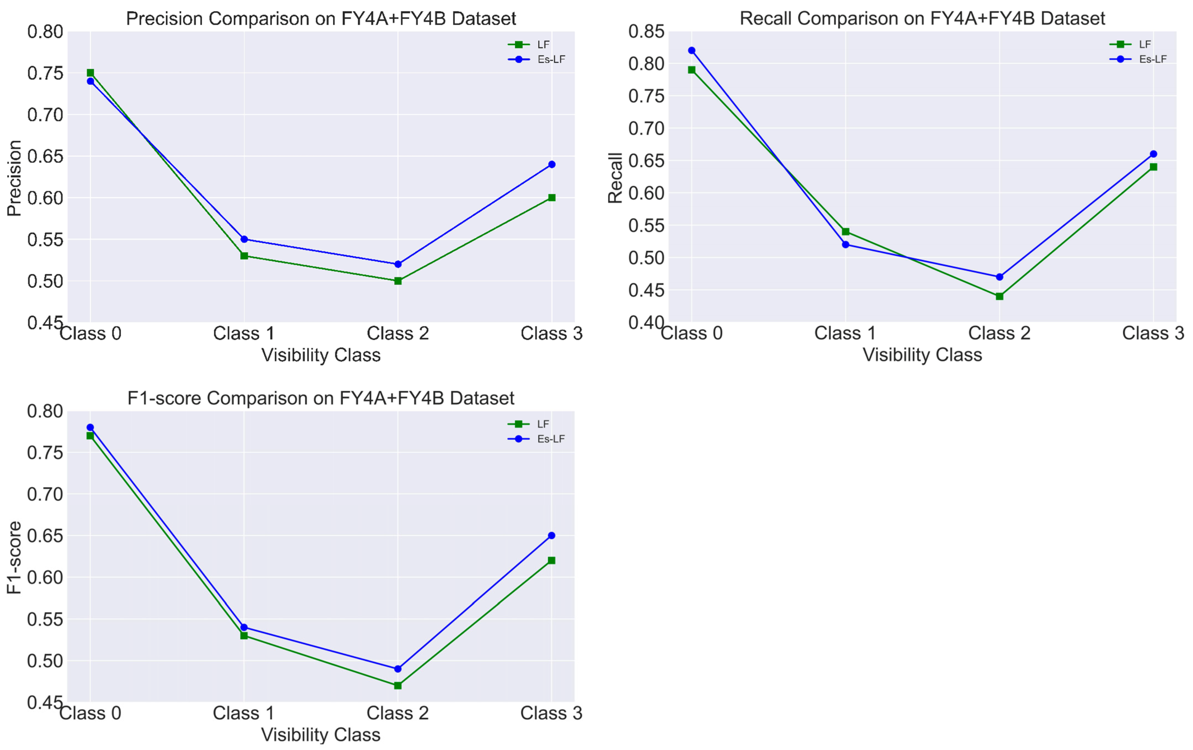
On this basis, we further summarized the Precision, Recall, and F1-score values of the original LF-Transformer and the ensemble LF-Transformer on the FY4A+FY4B fused dataset and compiled them into a comparison table, as shown in

Table 5. Performance Comparison of LF-Transformer and Ensembled LF-Transformer on the FY4A+FY4B Dataset.

FY4A+FY4B
	Precision		Recall		F1-Score
	LF	Es-LF	LF	Es-LF	LF	Es-LF
0	0.75	0.74	0.79	0.82	0.77	0.78
1	0.53	0.55	0.54	0.52	0.53	0.54
2	0.50	0.52	0.44	0.47	0.47	0.49
3	0.60	0.64	0.64	0.66	0.62	0.65

, to quantitatively demonstrate the performance improvements introduced by the ensemble strategy. Subsequently, we plotted the Precision, Recall, and F1-score curves for both models across different visibility levels to more intuitively illustrate the performance differences and trends, as shown in Figure 9. In general, Figure 9 demonstrates that the ensemble strategy provides a comprehensive and consistent performance improvement, particularly in Recall and F1-score. Specifically, although Precision in the dense or thick fog category (Class 0) slightly decreased (from 0.75 to 0.74), Recall increased from 0.79 to 0.82, and F1-score rose slightly from 0.77 to 0.78, indicating better recall capability and balanced performance.

For other categories, Precision improved across the board—for example: heavy fog (Class 1) increased from 0.53 to 0.55, moderate fog (Class 2) from 0.50 to 0.52, and clear weather without fog or haze (Class 3) from 0.61 to 0.64 —demonstrating enhanced discriminative ability of the ensemble model.

In terms of Recall, all categories showed improvement except for Class 1, which slightly decreased (from 0.54 to 0.52). Notably, moderate fog (Class 2) increased from 0.44 to 0.47, and clear weather (Class 3) from 0.64 to 0.66, suggesting that the ensemble model is more sensitive to minority and boundary samples, effectively reducing the risk of missed detections.

F1-scores also increased for all classes—from 0.53, 0.47, and 0.62 to 0.54, 0.49, and 0.65, respectively—reflecting the model’s balanced improvement in both accuracy and recall.

In summary, the ensemble LF-Transformer achieved robust and consistent improvements across multiple metrics, validating the significant effectiveness of ensemble learning for remote sensing-based visibility classification tasks.

In the spatial prediction task for typical visibility events, the ensembled LF-Transformer model maintains higher classification accuracy over a large spatial domain, with particularly strong performance for dense fog (Class 0) and moderate fog (Class 2). The corresponding spatial prediction results are shown in Supplementary Figure S3. The corresponding misclassification rates are 24% and 48%, representing reductions of 3% and 4%, respectively, compared with the original model. In contrast, the original model frequently exhibited class boundary misjudgments in transition regions (e.g., misclassifying Class 2 moderate fog as Class 1 heavy fog). The ensembled model significantly reduces both misclassification and omission errors, demonstrating its stronger spatial generalization ability in dealing with ambiguous class boundaries and imbalanced sample distributions in complex visibility scenarios.

In summary, the ensemble training not only improved numerical performance metrics but also enhanced class discrimination and spatial consistency, exhibiting greater robustness and adaptability. Compared with traditional machine learning methods, the LF-Transformer—leveraging its deep architecture and multi-head attention mechanism—can effectively capture multi-scale nonlinear features in remote sensing data. By introducing the ensemble strategy, the model further mitigates class confusion, improves stability and reliability in complex remote sensing environments, and demonstrates strong potential for intelligent visibility classification applications.

3.5. Computational Efficiency and Operational Deployability Analysis

Following the spatial inversion analysis of a typical low-visibility case, this study further evaluates the computational efficiency and operational deployability of the three models to assess their potential for real-time visibility monitoring. All experiments were conducted on a unified hardware platform equipped with an NVIDIA A30 GPU.

In terms of computational cost, the LF-Transformer used in this study contains 36,598,616 trainable parameters, representing a mid-sized Transformer architecture. Although its parameter scale is considerably larger than that of the lightweight Random Forest and Saint models, the LF-Transformer still demonstrates favorable efficiency during inference. Its single-sample inference latency ranges between 8–15 ms, with a peak GPU memory usage of approximately 0.8–1.5 GB. For the complete test set of 2800 samples, batch inference with a batch size of 50 requires only 4–6 s, indicating strong throughput performance sufficient to meet the real-time, minute-level update requirements of operational visibility monitoring systems.

Regarding training cost, the LF-Transformer required 34 min and 59 s to complete 100 training epochs on the A30 GPU, which remains within an acceptable range for operational applications. Although its training time is noticeably longer than that of Random Forest and Saint, the LF-Transformer exhibits substantially stronger multi-channel feature modeling capacity and better generalization stability. On the test set, the model achieved a 60% classification accuracy, with F1-scores of 0.77 (Class 0), 0.53 (Class 1), 0.47 (Class 2), and 0.62 (Class 3), indicating superior capability in identifying extremely low-visibility regions.

Random Forest, as a traditional statistical learning method, provides the fastest inference speed with the lowest memory consumption, while the Saint model—owing to its lightweight architecture—also delivers higher inference efficiency compared with the LF-Transformer. However, these computational advantages come at the cost of significantly reduced predictive performance. Both Random Forest and Saint exhibit low quantitative accuracy, blurred fog boundaries, and poor spatial consistency, making them unsuitable for fine-grained visibility classification under complex low-visibility conditions. In comparison, the LF-Transformer achieves improvements of approximately 12% in precision, 13% in recall, and 12% in F1-score, and shows markedly better performance in preserving spatial structures, identifying extreme low-visibility events, and maintaining cross-regional stability, thereby striking a more effective balance between computational cost and predictive performance.

From a deployment perspective, the inference latency, memory usage, and throughput of the LF-Transformer all fall within the acceptable range for current operational platforms such as traffic monitoring and meteorological early-warning systems that commonly utilize A30 GPUs. Its high stability and accuracy under low-visibility conditions provide strong support for fog monitoring and early-warning applications. Additionally, further optimizations—such as model pruning, knowledge distillation, and mixed-precision inference—may reduce computational overhead and enhance adaptability in broader operational environments.

In summary, considering both training and inference efficiency, the LF-Transformer achieves significant performance gains in multi-source remote sensing visibility classification while maintaining manageable computational requirements. It represents a highly accurate, scalable, and operationally valuable solution. Although Random Forest and Saint offer advantages in computational efficiency, their limitations in recognizing complex fog structures restrict their applicability in high-precision operational scenarios.

4. Discussion

Based on fused observations from the FY-4A and FY-4B geostationary meteorological satellites, this study constructed a remote-sensing visibility classification dataset and introduced the LF-Transformer model, which integrates frequency-domain and spatial attention mechanisms. The model was systematically compared with the traditional Random Forest model and the Saint model. Comprehensive experiments conducted on multiple data subsets and visibility levels lead to the following key findings.

4.1. Analysis of Model Generalization

To examine the applicability of the proposed model under different geographical and climatic conditions, the model constructed for the Jia–Shao Bridge region was further transferred and validated on the FY4A+FY4B fused dataset over Anhui Province. Compared with coastal areas, Anhui Province is characterized primarily by plains and hilly terrain, providing a representative testbed for evaluating the generalization capability of the model. The validation results are summarized in

Table 6. Performance Comparison of LF-Transformer, Random Forest, and Saint on the FY4A+FY4B Anhui Dataset.

FY4A+FY4B
	Precision			Recall			F1-Score
	LF	RF	Saint	LF	RF	Saint	LF	RF	Saint
0	0.75	0.63	0.55	0.78	0.57	0.68	0.76	0.60	0.65
1	0.55	0.36	0.47	0.56	0.35	0.28	0.56	0.38	0.31
2	0.52	0.32	0.43	0.48	0.42	0.40	0.49	0.41	0.40
3	0.61	0.54	0.53	0.62	0.58	0.58	0.60	0.53	0.57

.

The results show that the LF-Transformer exhibits more stable performance across all visibility levels in the Anhui region. In the dense or thick fog category (Class 0), the LF-Transformer achieves a precision of 0.75, which is significantly higher than that of the Random Forest model at 0.63 and the Saint model at 0.55. In the heavy fog (Class 1) and moderate fog (Class 2), the precision values of all models decrease; however, the LF-Transformer maintains relatively higher and more balanced precision levels across these visibility ranges. Under clear-weather conditions (Class 3), the LF-Transformer attains a precision of 0.61, outperforming Random Forest with 0.54 and Saint with 0.53. Overall, the validation results over Anhui Province demonstrate that the LF-Transformer preserves stable accuracy across different visibility levels, reflecting its effective learning of the physical relationship between satellite radiance features and atmospheric visibility.

In addition, to evaluate the model performance under different regional conditions, an independent low-visibility case over Anhui Province was analyzed. The corresponding spatial inversion results are presented in Supplementary Figure S4, which shows the predictions of the LF-Transformer, Random Forest, and Saint models over Anhui Province, respectively.

Based on the FY4A+FY4B fused dataset, the three models exhibit distinct misclassification characteristics across different visibility levels in Anhui Province. Overall, the LF-Transformer maintains lower misclassification rates across all four visibility classes, while the Random Forest shows relatively higher misclassification rates, and the Saint model performs between the two.

Under dense or thick fog conditions (Class 0), the misclassification rate of the LF-Transformer is 24%, which is substantially lower than that of the Random Forest at 40% and the Saint model at 35%, indicating more stable performance in extreme low-visibility scenarios. For heavy fog conditions (Class 1), the misclassification rates of all three models increase, with the LF-Transformer exhibiting a misclassification rate of 43%, which remains clearly lower than those of the Random Forest at 58% and the Saint model at 54%. Under moderate fog conditions (Class 2), the misclassification rate of the LF-Transformer reaches 51%, still lower than the Random Forest at 59% and the Saint model at 61%. This visibility level is characterized by higher uncertainty in radiative features and spatial structures, making it a common source of confusion for all models. Under clear-weather conditions (Class 3), the overall misclassification rates decrease, with the LF-Transformer achieving a rate of 32%, compared with 42% for the Random Forest and 39% for the Saint model, again demonstrating the best performance among the three.

Overall, the analysis over Anhui Province indicates that the LF-Transformer maintains stable inversion performance under independent regional conditions, further confirming its effectiveness and generalization capability across different regional backgrounds.

4.2. Comparison with Recent Multimodal Visibility Prediction Approaches

To further contextualize the above results and clarify the methodological positioning of our station–satellite framework, we compare our approach with representative recent multimodal visibility recognition studies.

Wang et al. addressed airport visibility recognition during nighttime and early morning by proposing an image–tabular multimodal fusion framework. In the image branch, to alleviate the lack of information under low-light conditions, the original images, pseudo-color enhanced images, and Sobel edge maps are fused to explicitly introduce discriminative cues such as illumination and edge structures. Subsequently, image features are extracted using EfficientNetB1, while tabular meteorological variables are encoded using an FT-Transformer. In the fusion stage, multimodal classification is performed via feature concatenation (late fusion) followed by an MLP classifier. Overall, this study follows an engineering-oriented pipeline characterized by image enhancement, independent dual-branch feature encoding, and late-stage feature fusion.

In contrast to such ground-camera-based multimodal approaches, this study focuses on the fusion of station-based visibility observations and FY-4 multi-channel satellite measurements. The input data take the form of station-collocated multi-channel satellite tabular features, rather than being limited to camera views at a small number of airport locations. Compared with ground-based cameras, which are constrained by deployment conditions, limited spatial coverage, and sensitivity to local illumination and occlusion, FY-4 satellite observations provide broader spatial coverage and continuous, operationally stable measurements. This enables the provision of consistent multi-channel radiance information at the regional scale, offering a more generally applicable remote-sensing basis for low-visibility monitoring and early warning. From a modeling perspective, cross-modal relationships in Wang et al.’s framework are mainly learned implicitly by the downstream MLP operating on concatenated features. By contrast, this study introduces and adopts the existing LF-Transformer (Line/Factorized Transformer) as the core modeling framework. Through directional encoding (row-wise and column-wise encoding) and explicit interaction-fusion modules, the LF-Transformer directly models inter-channel dependencies and higher-order interactions in a structured latent space. This design is better suited to satellite observations that exhibit strong inter-channel correlations, pronounced noise/outliers, and scarce low-visibility samples that are easily confused with low clouds and haze, which is consistent with the more stable cross-regional generalization observed in our experiments.

4.3. Model Limitations and Future Directions

Despite its outstanding overall performance, the LF-Transformer still shows lower F1-scores of 0.53 for the heavy fog category (Class 1), indicating that deep learning models continue to struggle with ambiguous class boundaries and overlapping feature distributions. Furthermore, the Transformer architecture involves substantial computational cost, which may hinder deployment in resource-limited operational environments.

To further enhance model performance, future research can explore the following directions:

(1) Introducing additional data sources—such as weather radar, traffic sensors, or ground-based observation systems to enrich the feature space.

(2) Adopting adaptive sample re-weighting or boundary-enhancement methods to improve separation between overlapping visibility classes.

(3) Exploring lighter or more efficient Transformer variants to reduce computational overhead and enhance deployability in operational systems.

(4) Conducting systematic validation over a wider range of typical regions—such as mountainous areas, hilly terrain, and plateau transition zones—to further assess model robustness and generalization capability under diverse geographic and climatic conditions.

In addition, although the lightweight ensemble strategy improves model stability, there remains room for further optimization in mid-visibility classification performance.

5. Conclusions

This study proposes a visibility classification framework based on FY-4A/FY-4B fused data and the LF-Transformer model. Through comprehensive comparisons with the Random Forest and Saint models, the main conclusions are as follows:

(1) The LF-Transformer consistently outperforms Random Forest and Saint in visibility classification, demonstrating higher discrimination stability and robustness, particularly under low-visibility conditions.

(2) The fusion of FY-4A and FY-4B observations significantly improves the consistency and stability of classification results. Compared with using FY-4A alone, the fused dataset yields superior performance across all visibility categories, confirming the practical value of dual-satellite fusion for operational visibility monitoring.

(3) SHAP-based interpretability analysis indicates that the model primarily relies on key spectral channels closely related to water vapor and cloud physical processes, demonstrating good consistency between the model’s decision logic and underlying atmospheric physics.

(4) The ensemble version of the LF-Transformer further enhances prediction stability, indicating strong potential for regional-scale visibility monitoring, early warning, and traffic safety applications.

Overall, the LF-Transformer provides a powerful, interpretable, and scalable framework for visibility classification based on multi-source remote sensing, demonstrating substantial application potential in meteorological monitoring, traffic safety, and visibility forecasting.

References

1. Ye, P. Remote sensing approaches for meteorological disaster monitoring: Recent achievements and new challenges. Int. J. Environ. Res. Public Health 2022, 19, 3701. [Google Scholar] [CrossRef] [PubMed]
2. Janga, B.; Asamani, G.P.; Sun, Z.; Cristea, N. A review of practical AI for remote sensing in earth sciences. Remote Sens. 2023, 15, 4112. [Google Scholar] [CrossRef]
3. Zhang, C.; Wu, M.; Chen, J.; Chen, K.; Zhang, C.; Xie, C.; Huang, B.; He, Z. Weather visibility prediction based on multimodal fusion. IEEE Access 2019, 7, 74776–74786. [Google Scholar] [CrossRef]
4. Kamangir, H.; Collins, W.; Tissot, P.; King, S.A.; Dinh, H.T.H.; Durham, N.; Rizzo, J. FogNet: A multiscale 3D CNN with double-branch dense block and attention mechanism for fog prediction. Mach. Learn. Appl. 2021, 5, 100038. [Google Scholar] [CrossRef]
5. Miclea, R.-C.; Dughir, C.; Alexa, F.; Sandru, F.; Silea, I. Laser and LIDAR in a system for visibility distance estimation in fog conditions. Sensors 2020, 20, 6322. [Google Scholar] [CrossRef] [PubMed]
6. Niu, Z.; Zhang, L.; Han, Y.; Dong, P.; Huang, W. Performances between the FY-4A/GIIRS and FY-4B/GIIRS long-wave infrared (LWIR) channels under clear-sky and all-sky conditions. Q. J. R. Meteorol. Soc. 2023, 149, 1612–1628. [Google Scholar] [CrossRef]
7. Huang, Y.; Bao, Y.; Petropoulos, G.P.; Lu, Q.; Huo, Y.; Wang, F. Precipitation estimation using FY-4B/AGRI satellite data based on random forest. Remote Sens. 2024, 16, 1267. [Google Scholar] [CrossRef]
8. Wen, D.; Huang, X.; Bovolo, F.; Li, J.; Ke, X.; Zhang, A.; Benediktsson, J.A. Change detection from very-high-spatial-resolution optical remote sensing images: Methods, applications, and future directions. IEEE Geosci. Remote Sens. Mag. 2021, 9, 68–101. [Google Scholar] [CrossRef]
9. Faust, J.A. PFAS on atmospheric aerosol particles: A review. Environ. Sci. Process. Impacts 2023, 25, 133–150. [Google Scholar] [CrossRef] [PubMed]
10. Amiri, M.; Soleimani, S. A hybrid atmospheric satellite image-processing method for dust and horizontal visibility detection through feature extraction and machine learning techniques. J. Indian Soc. Remote Sens. 2022, 50, 523–532. [Google Scholar] [CrossRef]
11. Speiser, J.L.; Miller, M.E.; Tooze, J.; Ip, E. A comparison of random forest variable selection methods for classification prediction modeling. Expert Syst. Appl. 2019, 134, 93–101. [Google Scholar] [CrossRef] [PubMed]
12. Sun, Z.; Wang, G.; Li, P.; Wang, H.; Zhang, M.; Liang, X. An improved random forest based on the classification accuracy and correlation measurement of decision trees. Expert Syst. Appl. 2024, 237, 121549. [Google Scholar] [CrossRef]
13. Liu, Z.; Chen, Y.; Gu, X.; Yeoh, J.K.; Zhang, Q. Visibility classification and influencing-factors analysis of airport: A deep learning approach. Atmos. Environ. 2022, 278, 119085. [Google Scholar] [CrossRef]
14. Wang, L.; Cui, Z.; Dong, S.; Wang, N. Airport Visibility Classification Based on Multimodal Fusion of Image-tabular Data. IEEE Access 2024, 12, 155082–155097. [Google Scholar] [CrossRef]
15. Gorishniy, Y.; Rubachev, I.; Khrulkov, V.; Babenko, A. Revisiting deep learning models for tabular data. Adv. Neural Inf. Process. Syst. 2021, 34, 18932–18943. [Google Scholar]
16. Wolf, T.; Debut, L.; Sanh, V.; Chaumond, J.; Delangue, C.; Moi, A.; Cistac, P.; Rault, T.; Louf, R.; Funtowicz, M.; et al. Transformers: State-of-the-art natural language processing. In Proceedings of the 2020 Conference on Empirical Methods in Natural Language Processing: System Demonstrations, Online, 16–20 November 2020; Association for Computational Linguistics: Kerrville, TX, USA, 2020; pp. 38–45. [Google Scholar]
17. Han, K.; Wang, Y.; Chen, H.; Chen, X.; Guo, J.; Liu, Z.; Tang, Y.; Xiao, A.; Xu, C.; Xu, Y.; et al. A survey on vision transformer. IEEE Trans. Pattern Anal. Mach. Intell. 2022, 45, 87–110. [Google Scholar] [CrossRef] [PubMed]
18. Chen, H.; Jiang, D.; Sahli, H. Transformer encoder with multi-modal multi-head attention for continuous affect recognition. IEEE Trans. Multimed. 2020, 23, 4171–4183. [Google Scholar] [CrossRef]
19. Han, K.; Xiao, A.; Wu, E.; Guo, J.; Xu, C.; Wang, Y. Transformer in transformer. Adv. Neural Inf. Process. Syst. 2021, 34, 15908–15919. [Google Scholar]
20. Soyalp, G.; Alar, A.; Ozkanli, K.; Yildiz, B. Improving text classification with transformer. In Proceedings of the 2021 6th International Conference on Computer Science and Engineering (UBMK), Ankara, Turkey, 15–17 September 2021; IEEE: New York, NY, USA, 2021; pp. 707–712. [Google Scholar]
21. Na, K.; Lee, J.-H.; Kim, E. Lf-transformer: Latent factorizer transformer for tabular learning. IEEE Access 2024, 12, 10690–10698. [Google Scholar] [CrossRef]
22. He, Y. LF Transformer: A novel lightweight network for machine translation. In Proceedings of the 2024 7th International Conference on Computer Information Science and Artificial Intelligence, Shaoxing, China, 13–15 September 2024; Association for Computing Machinery: New York, NY, USA, 2024; pp. 104–109. [Google Scholar]
23. Somepalli, G.; Goldblum, M.; Schwarzschild, A.; Bruss, C.B.; Goldstein, T. Saint: Improved neural networks for tabular data via row attention and contrastive pre-training. arXiv 2021, arXiv:2106.01342. [Google Scholar] [CrossRef]
24. GB/T 27964-2011; Grades of Fog Forecasting. China Meteorological Administration: Beijing, China, 2011.
Figure 1. Structure of the LF-Transformer Model.
Remotesensing 18 00618 g001
Figure 2. Distribution of Research Stations in Jiaxing and Shaoxing.
Remotesensing 18 00618 g002
Figure 3. Performance Comparison of LF-Transformer, Random Forest, and Saint on the FY4A+FY4B Fused Dataset.
Remotesensing 18 00618 g003
Figure 4. Comparison of Confusion Matrices among LF-Transformer, Random Forest, and Saint on the FY4A+FY4B Fused Dataset.
Remotesensing 18 00618 g004
Figure 5. Visualization of Misclassification Trends: Comparison of True and Predicted Sample Counts Across Classes for Different Models.
Remotesensing 18 00618 g005
Figure 6. Spatial Distribution of model predictions during a Typical Low-Visibility Event.
Remotesensing 18 00618 g006
Figure 7. Spatial distribution of prediction errors for the LF-Transformer under different visibility classes.
Remotesensing 18 00618 g007
Figure 8. Distribution of Feature Contribution Scores (SHAP Values) for the LF-Transformer Model.
Remotesensing 18 00618 g008
Figure 9. Performance Comparison between LF-Transformer and Ensemble LF-Transformer on the FY4A+FY4B Fused Dataset.
Remotesensing 18 00618 g009